Submitted:
16 August 2023
Posted:
18 August 2023
You are already at the latest version
Abstract
Keywords:
1. Introduction
2. Model and Data
3. Experiments
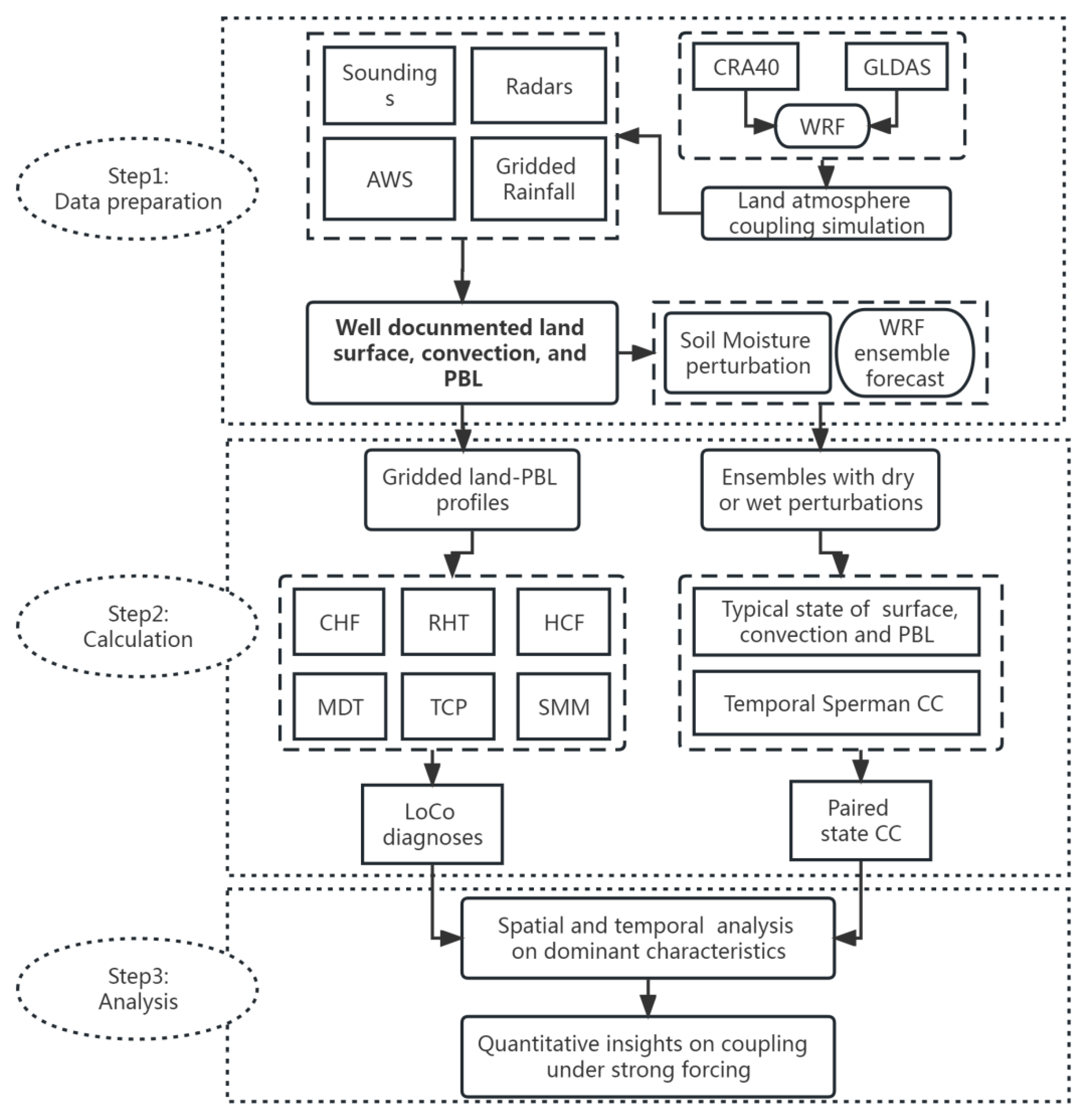
4. Methods
4.1. The local coupling metrics
4.2. The ensemble statistical metrics
| (1) | |
| (2) |
|
|
(3) |
5. Results
5.1. Simulation overview
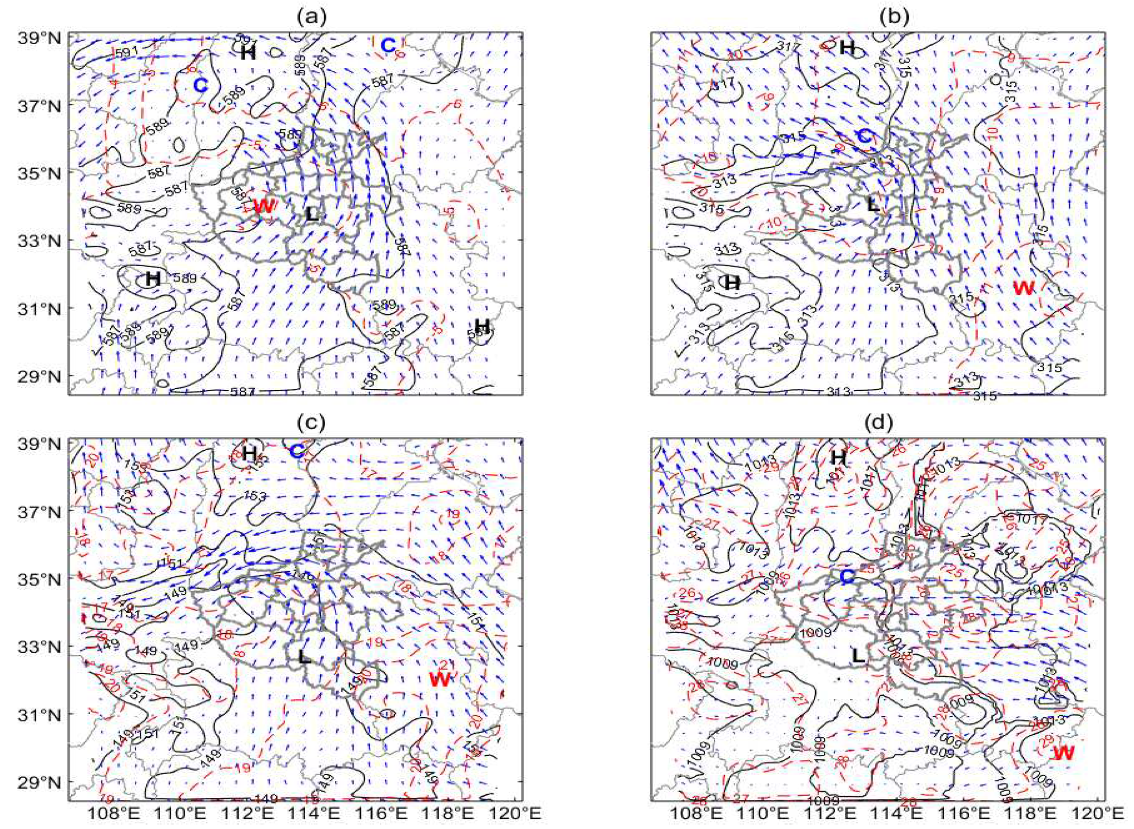
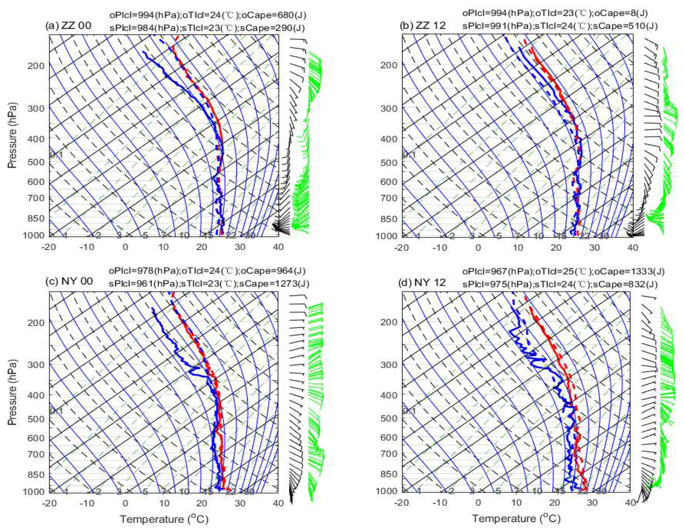
5.1.1. Synoptic and thermodynamics
5.1.2. Convection and rainfall
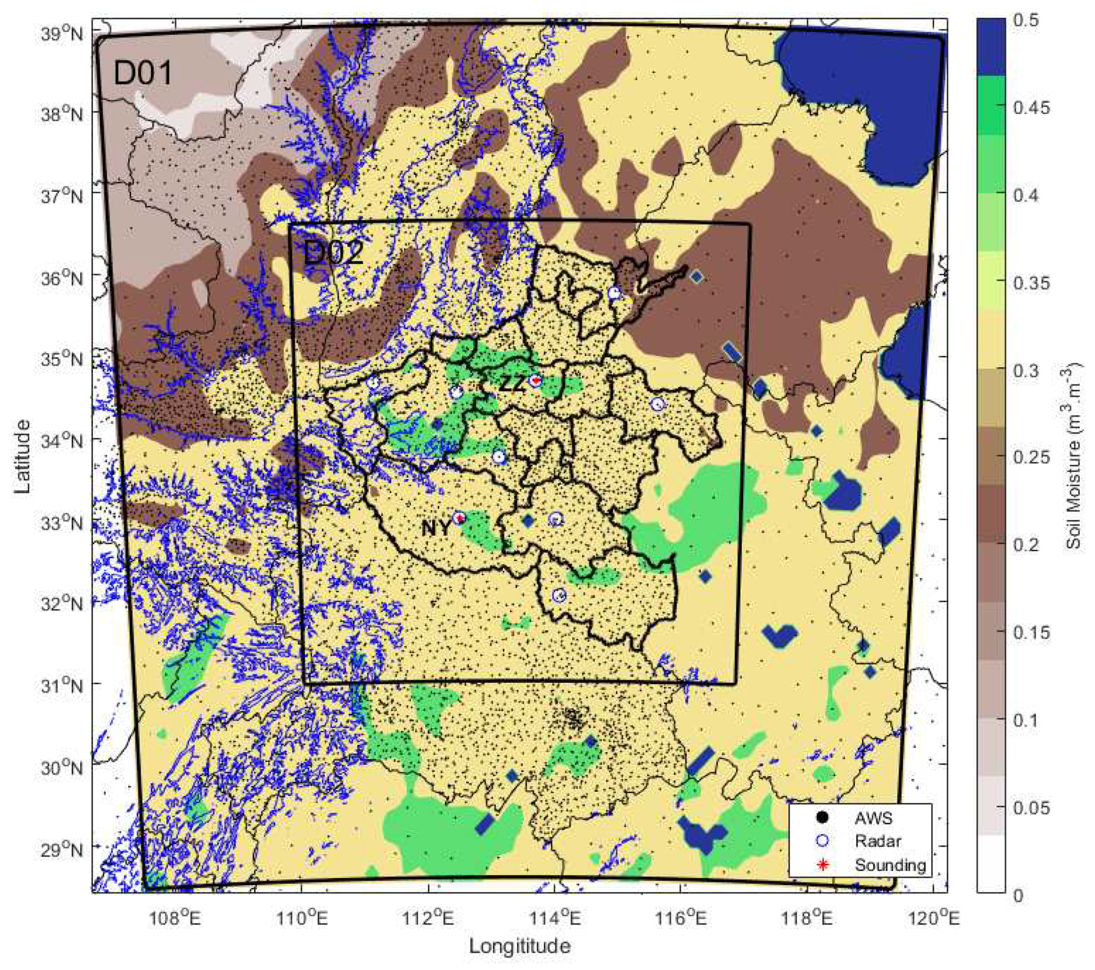
5.1.3. Underlying surface characteristics
5.2. The local coupling evaluation
5.2.1. CHF
5.2.2. RHT
5.2.3. HCF
5.2.4. MDT
5.2.5. TCP
5.2.6. SMM
5.3. The ensemble statistical relations
5.3.1. Spatially averaged relations
5.3.2. Point wised relations
6. Conclusions
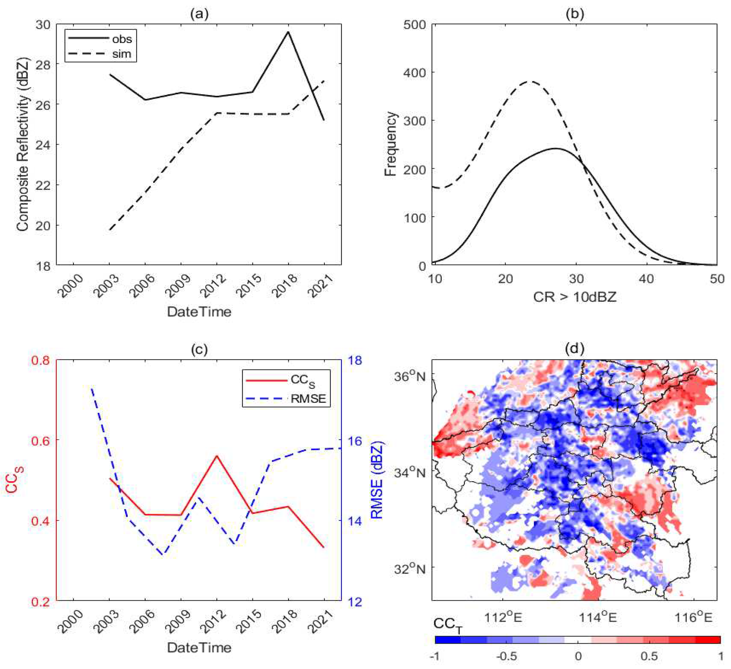
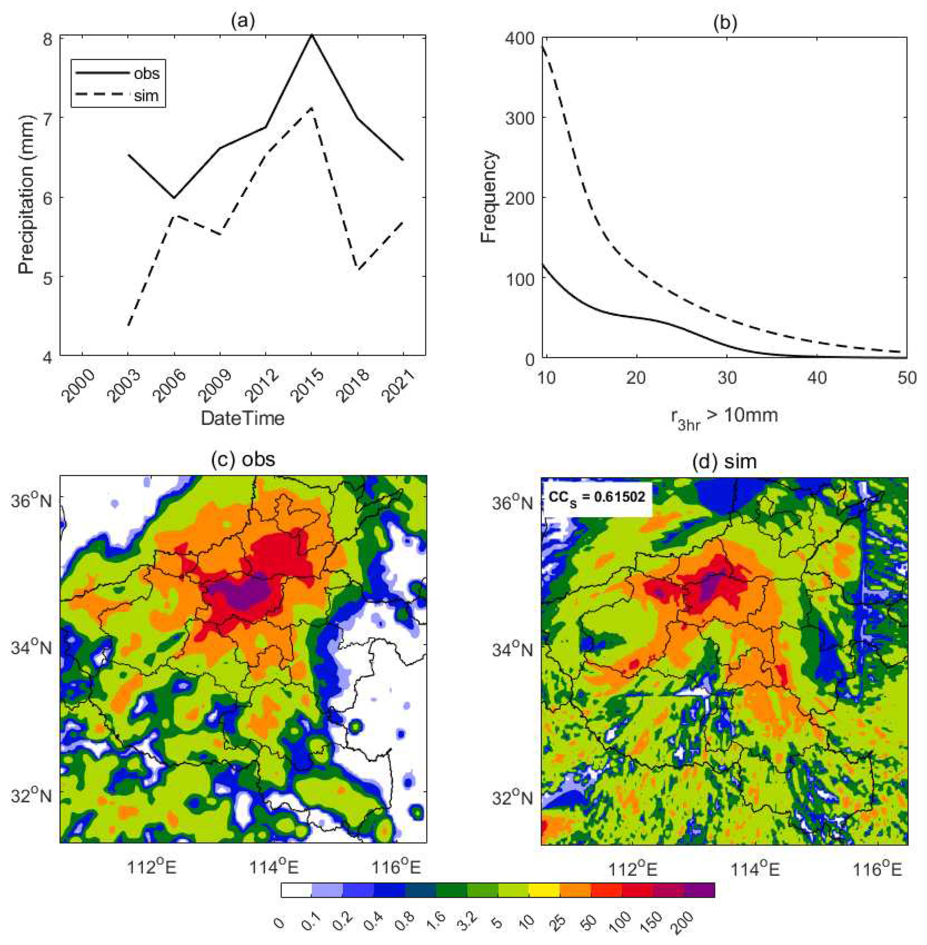
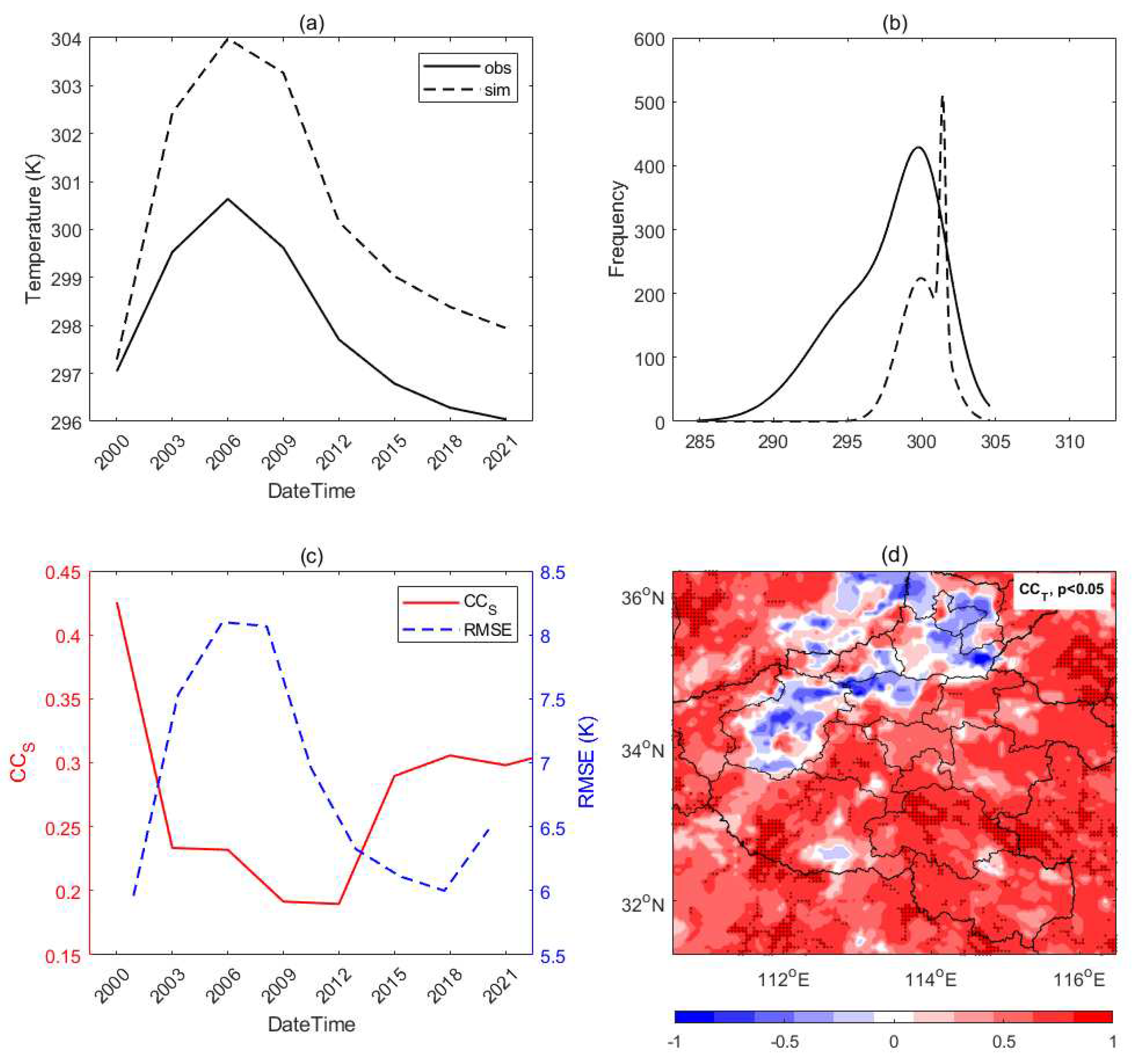
- The long-lasting low-value system with the upper warm flow and lower strong cold invading, the mid-low layer thermodynamic situations, the convection and rainfall spatiotemporal characteristics, and the diurnal surface thermal characteristics are consistent with the available observations. However, the stratospheric (higher than 400 hPa) thermodynamics that related to the northern developed rainfall and convection, and the during mountain areas have been found biased. Except for the mountain areas, the main characteristics during the low atmosphere and the surface can be well documented in this modeled event.
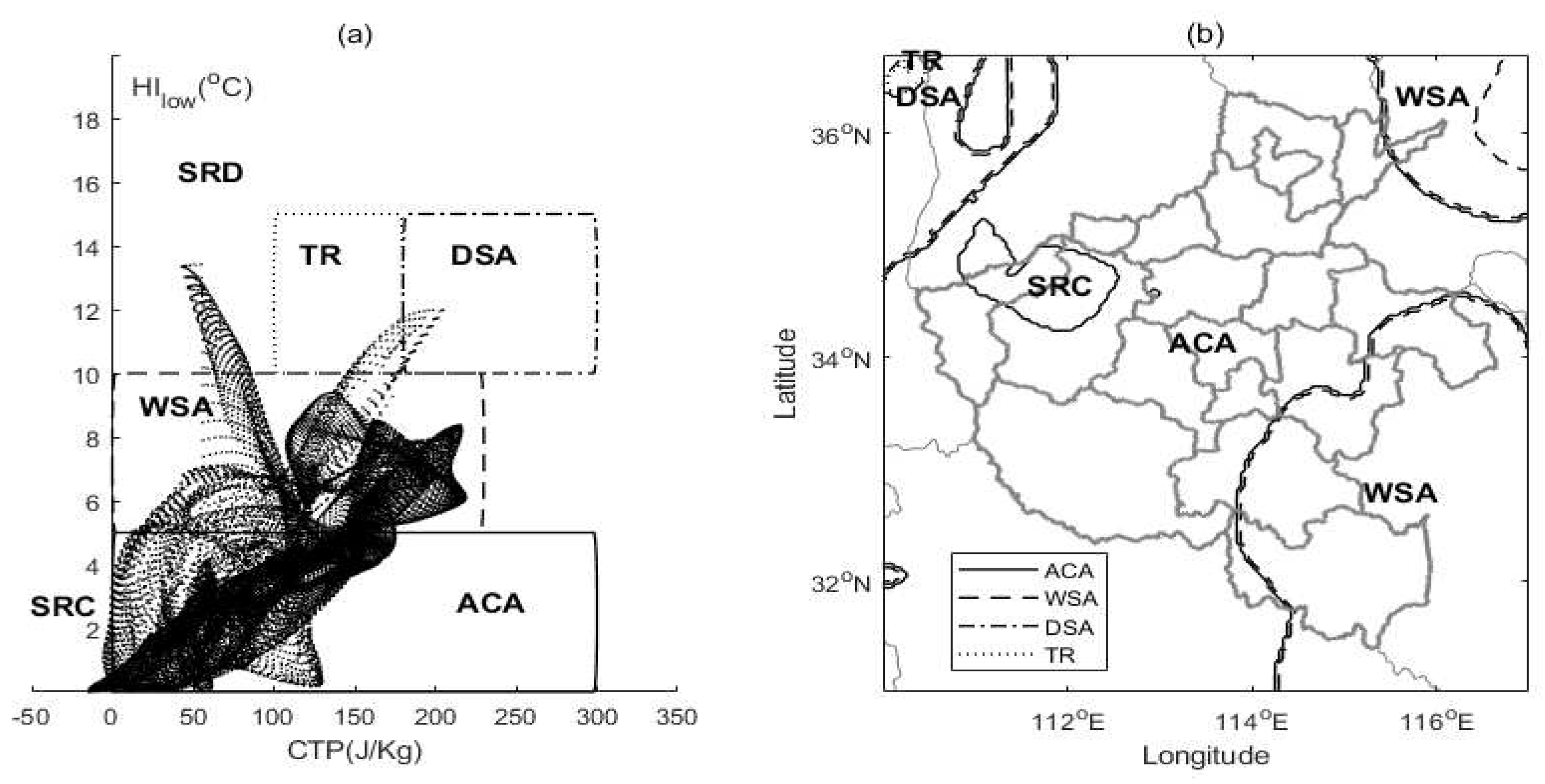
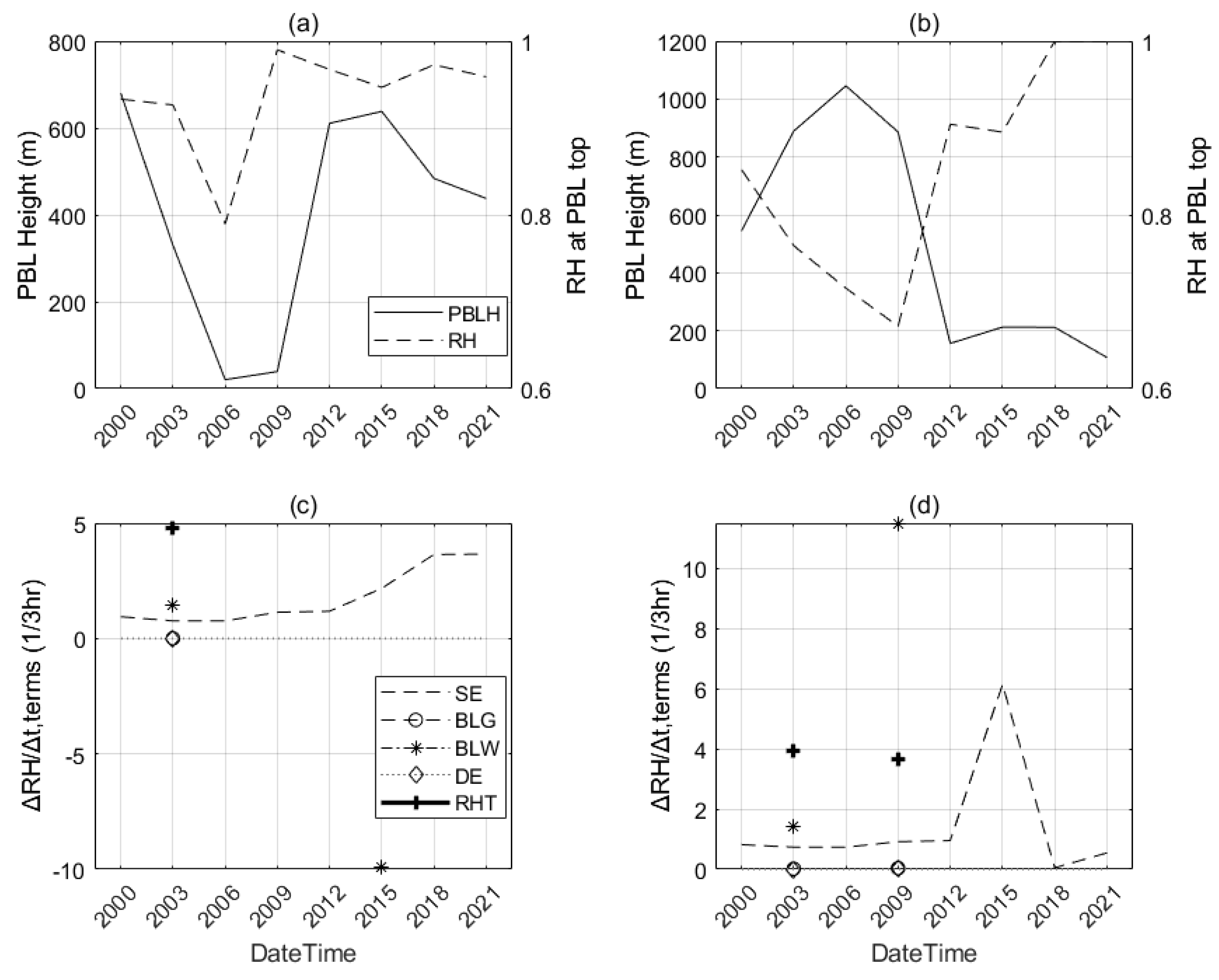
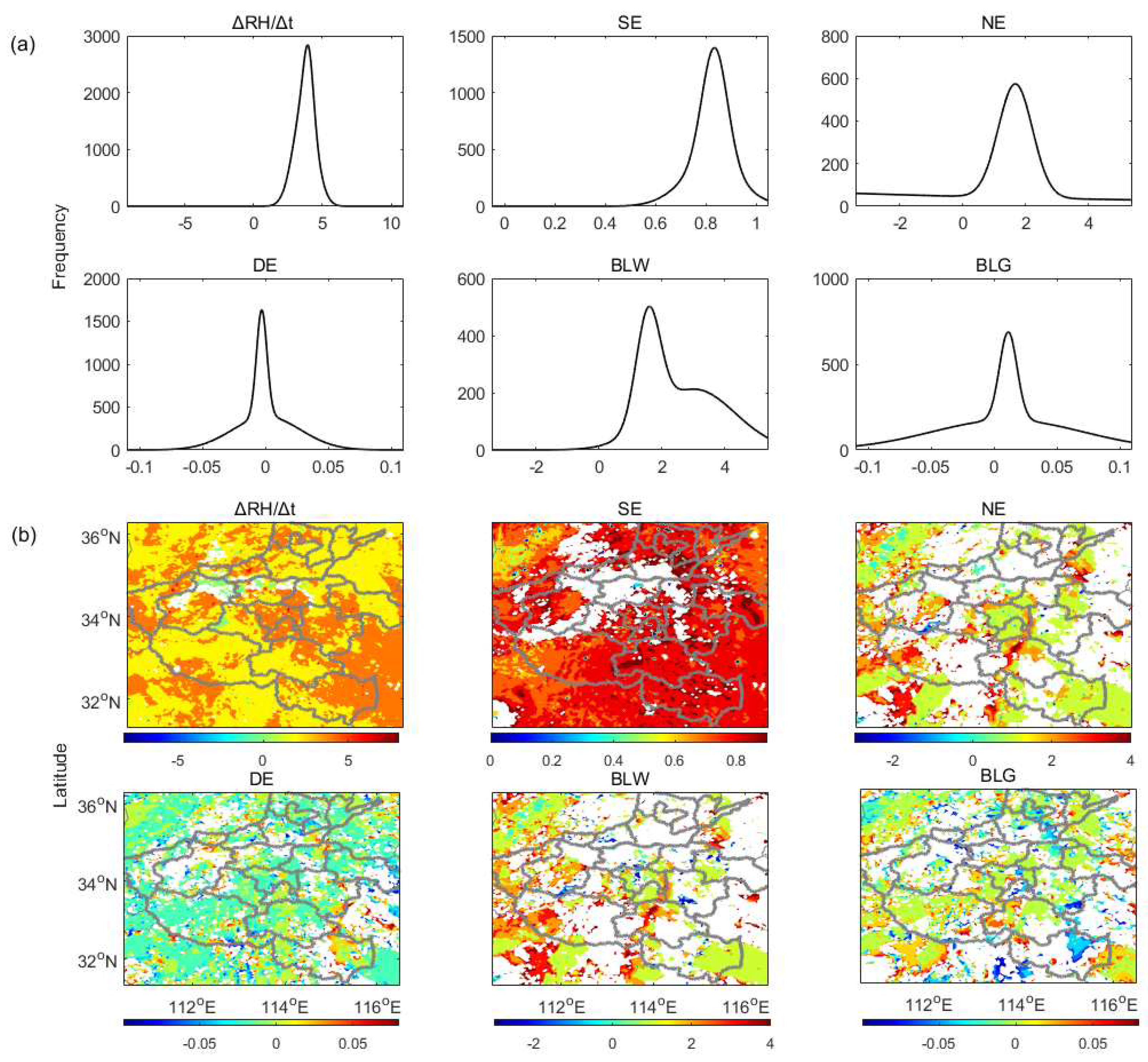
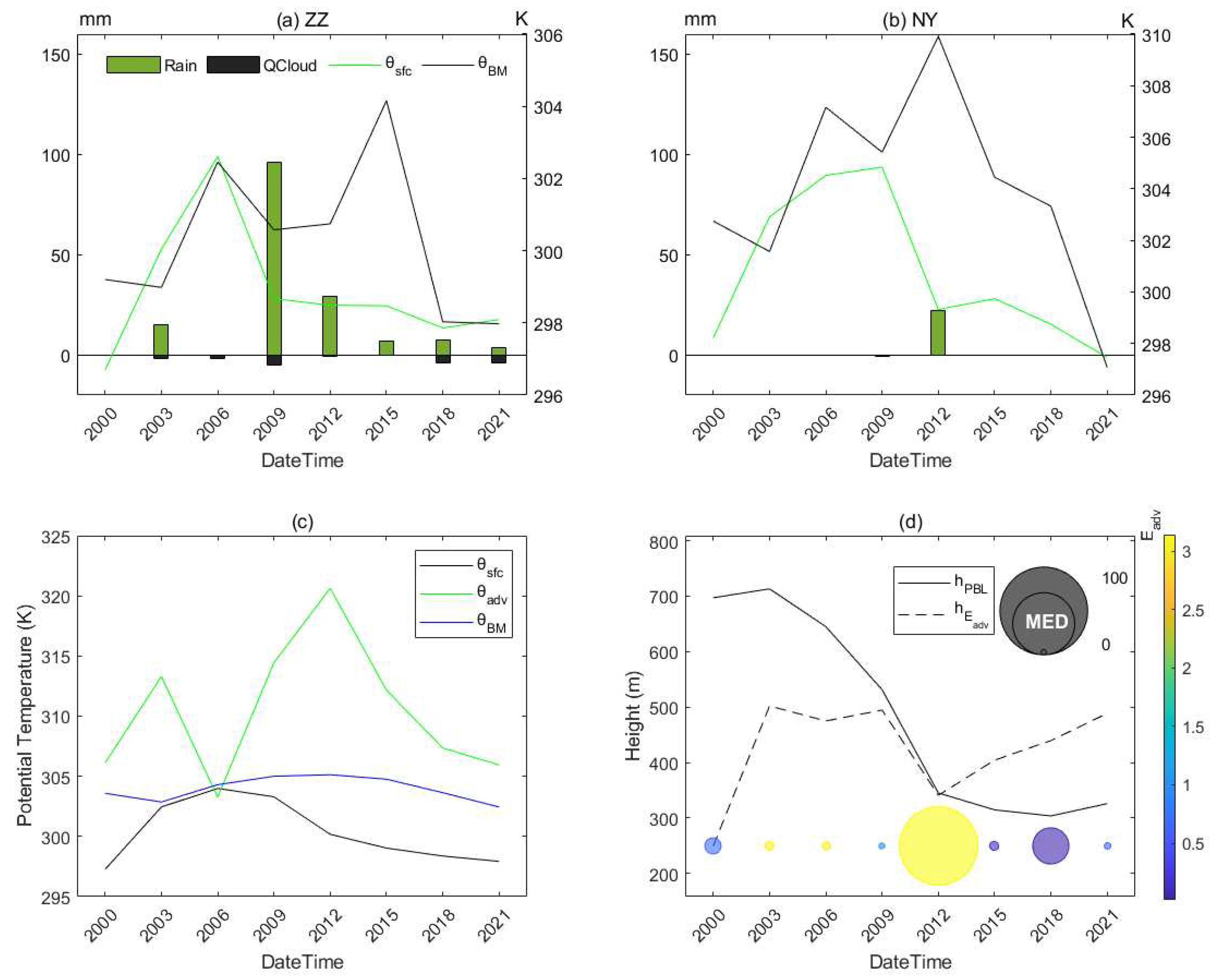
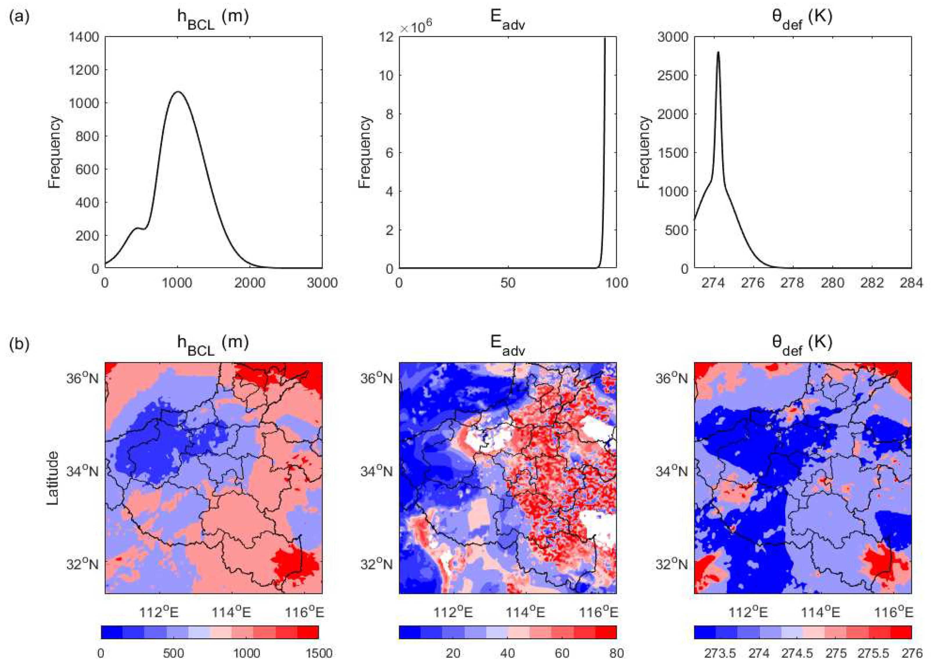
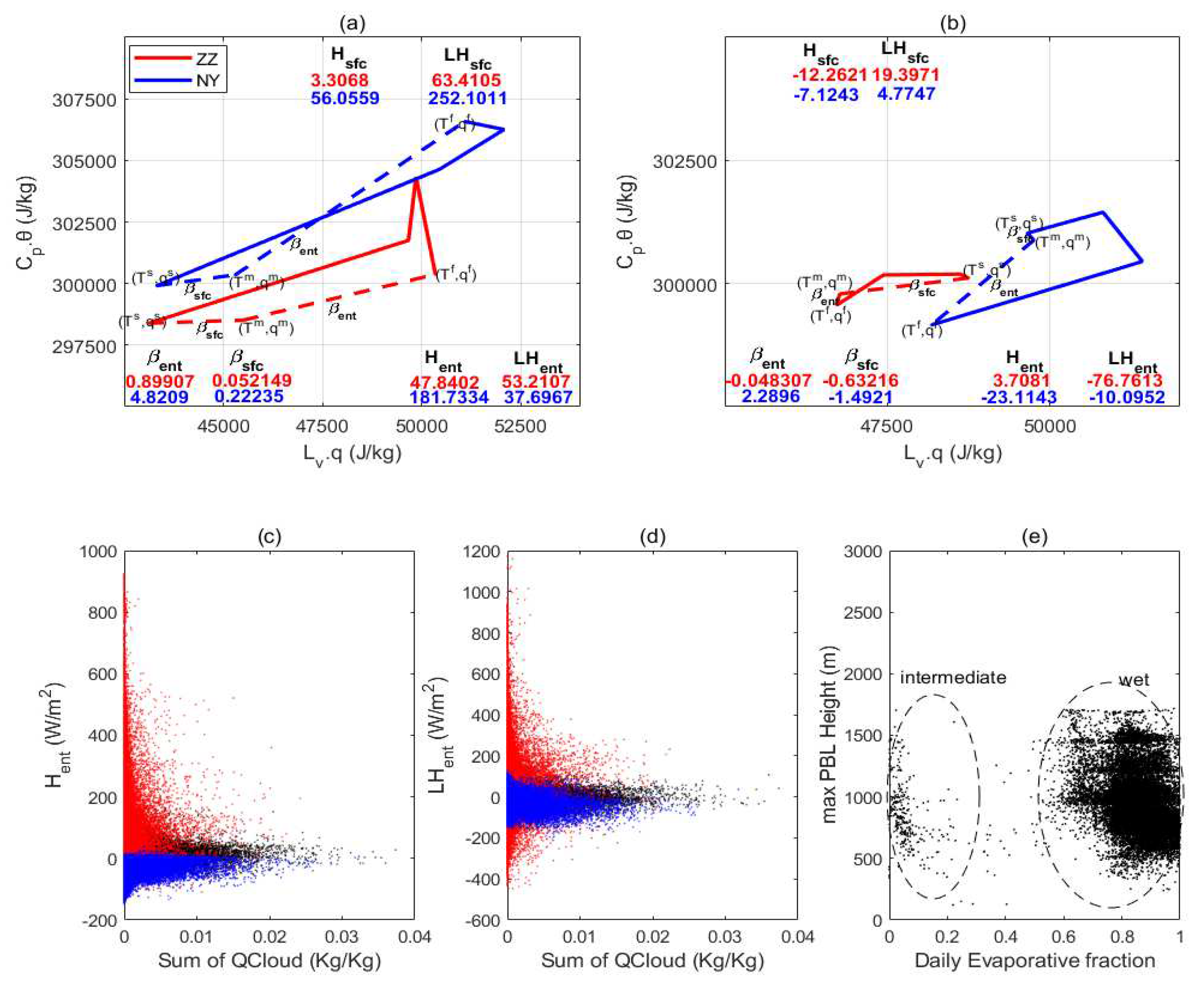
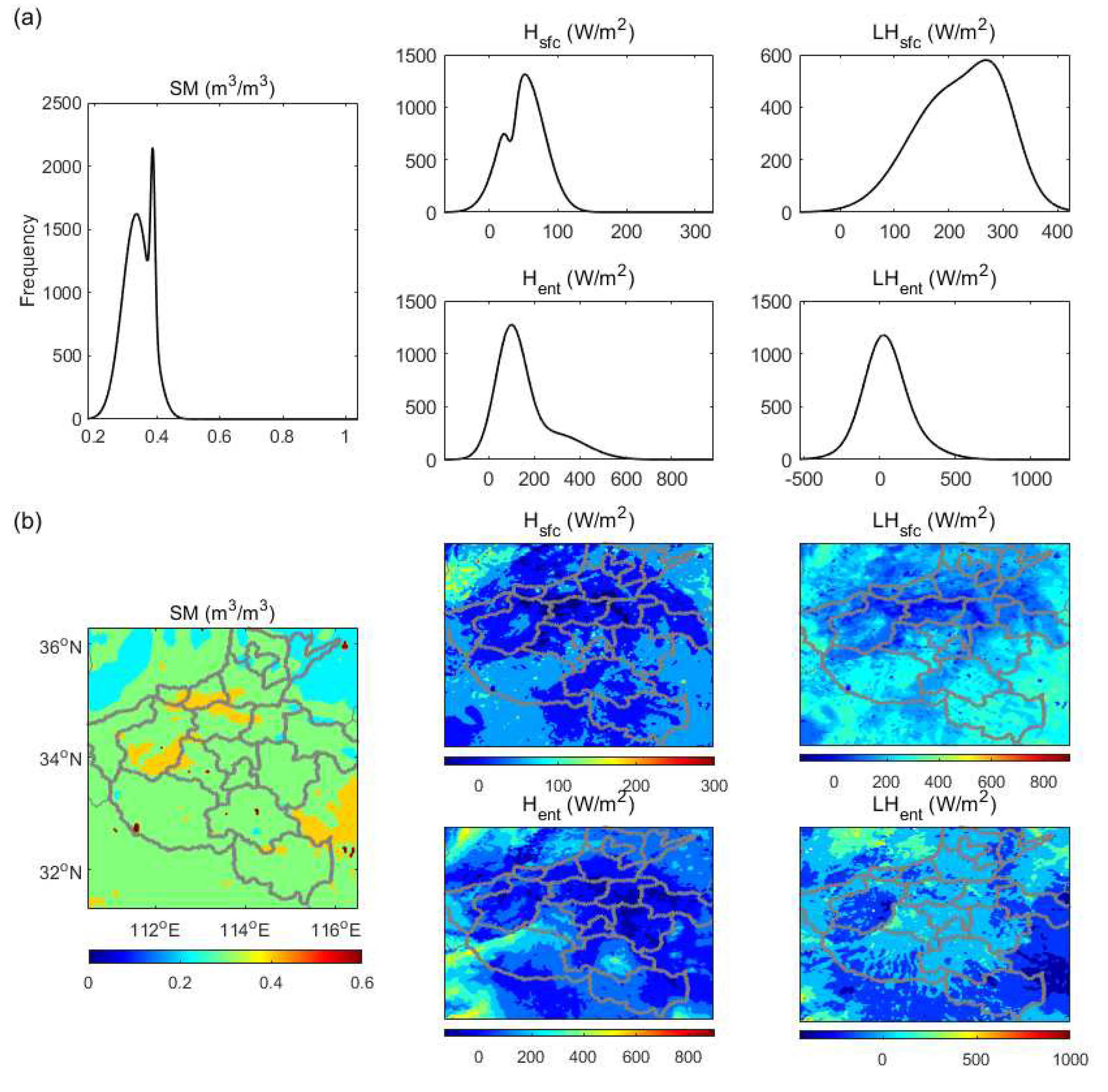
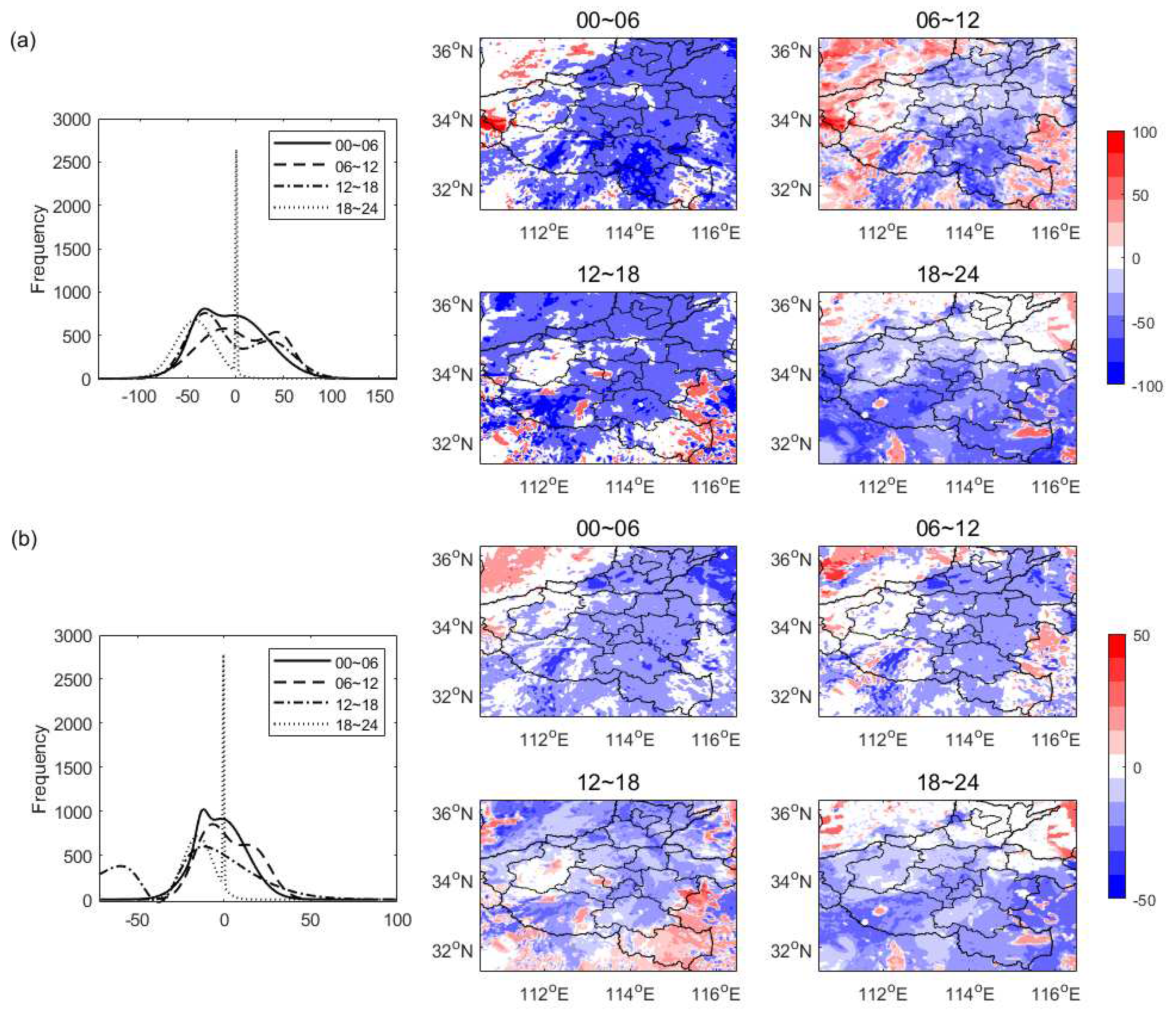
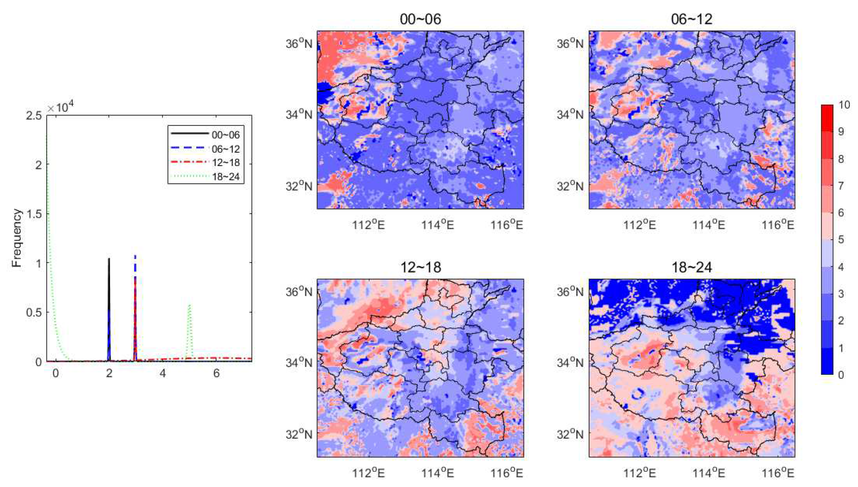
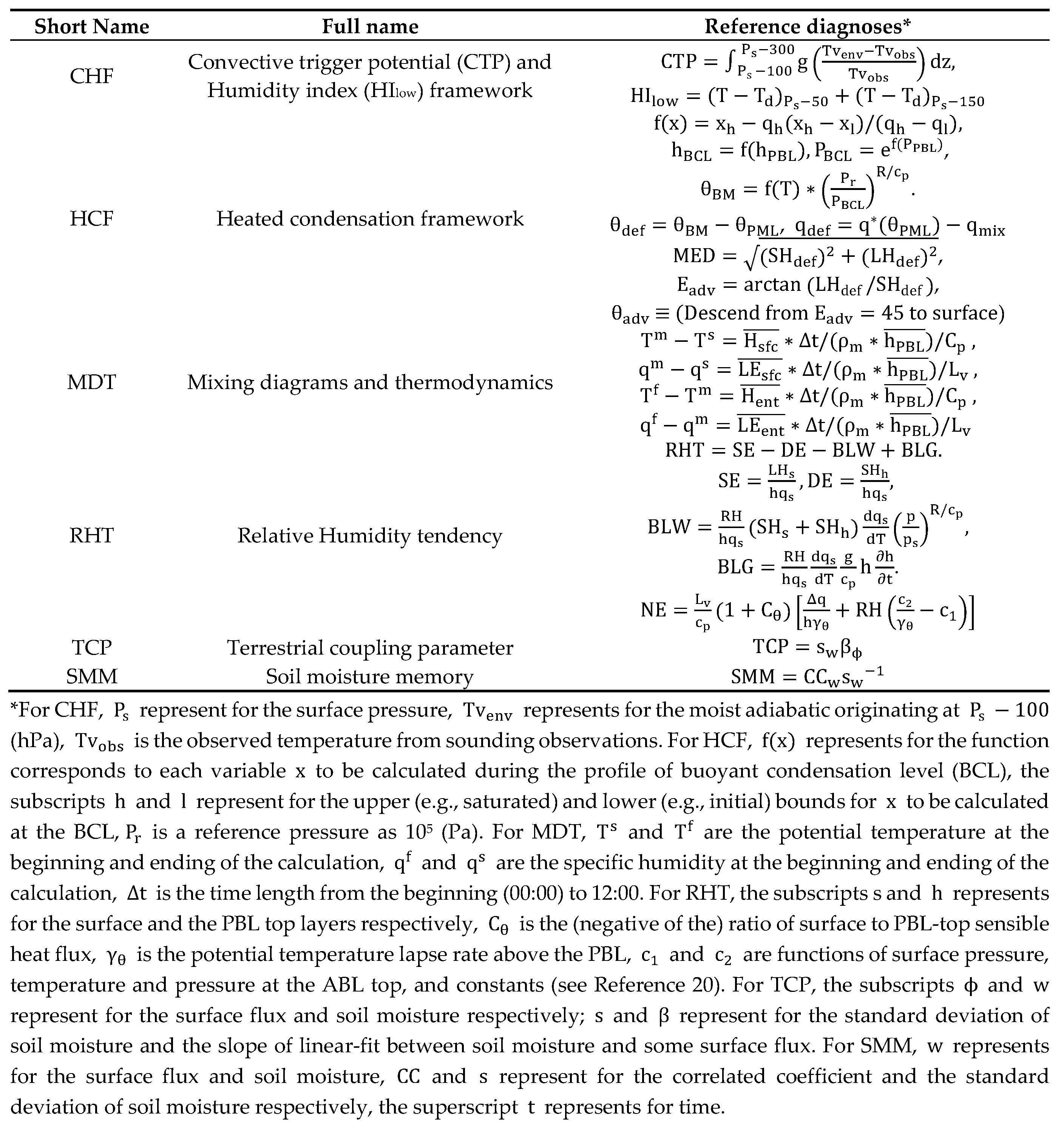
- In CHF, the PBL near the west of the storm center is likely too stable to rain (SRC), and thee PBL on the northwest needs additional CTP to trigger convection (TR) while other regions have shown different advantaged (e.g., ACA, WSA, and DSA) and are favor of afternoon convection. In RHT, great contributions to RHT from the surface evaporation (SE), PBL warming (BLW), and non-evaporative factors (NE) have indicated their dominant roles in the local PBL clouds developing before noontime, during which SE around 0.8 and NE around 2 are especially significant. In HCF, the noontime lower buoyant mixing temperature deficits (e.g, around 274K) with developing clouds could trigger the convection except in the SRC region, while the significant energy transform of PBL occurs when the main rainstorm ends and these have dominated the daytime PBL cloud developing but with regional differences. In MDT, both the daytime PBL and surface latent energy contributions around 100 and 280 W/m2 respectively have dominated the surface relations to PBL clouds, nevertheless, soil moisture and atmospheric forcing have greatly shaped the daytime surface fluxes distribution characterized as low entrainment heat flux () but high entrainment latent flux (). In TCP, surface coupling surrounding the middle east domain occurs in the local afternoon are significant during this event. In SMM, it has increased along with time, and the comparable distributions of both initial SM and developed rainfall at the end have indicated that both the surface soil and upper rainfall have shaped the spatial distribution of SMM.
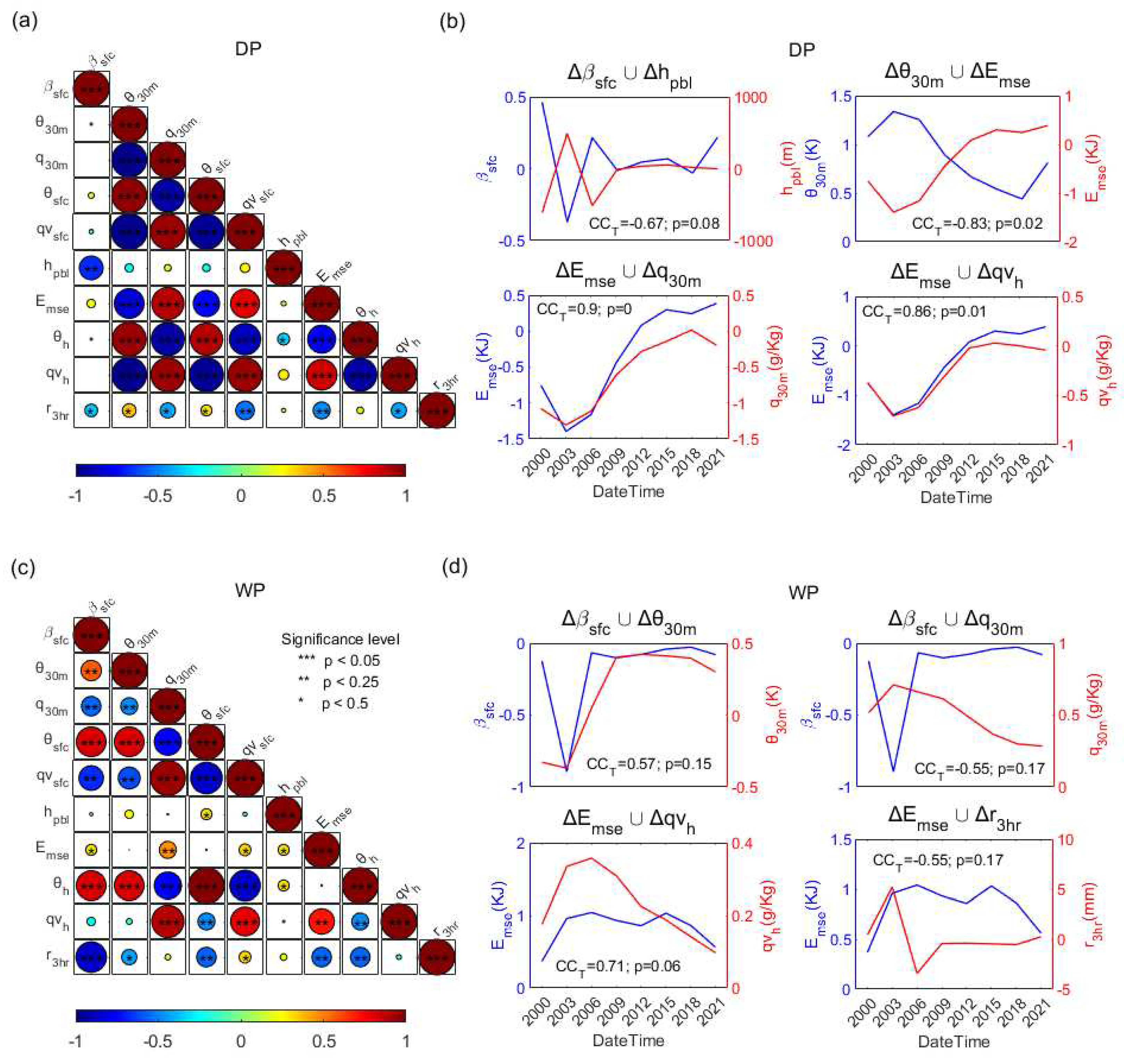
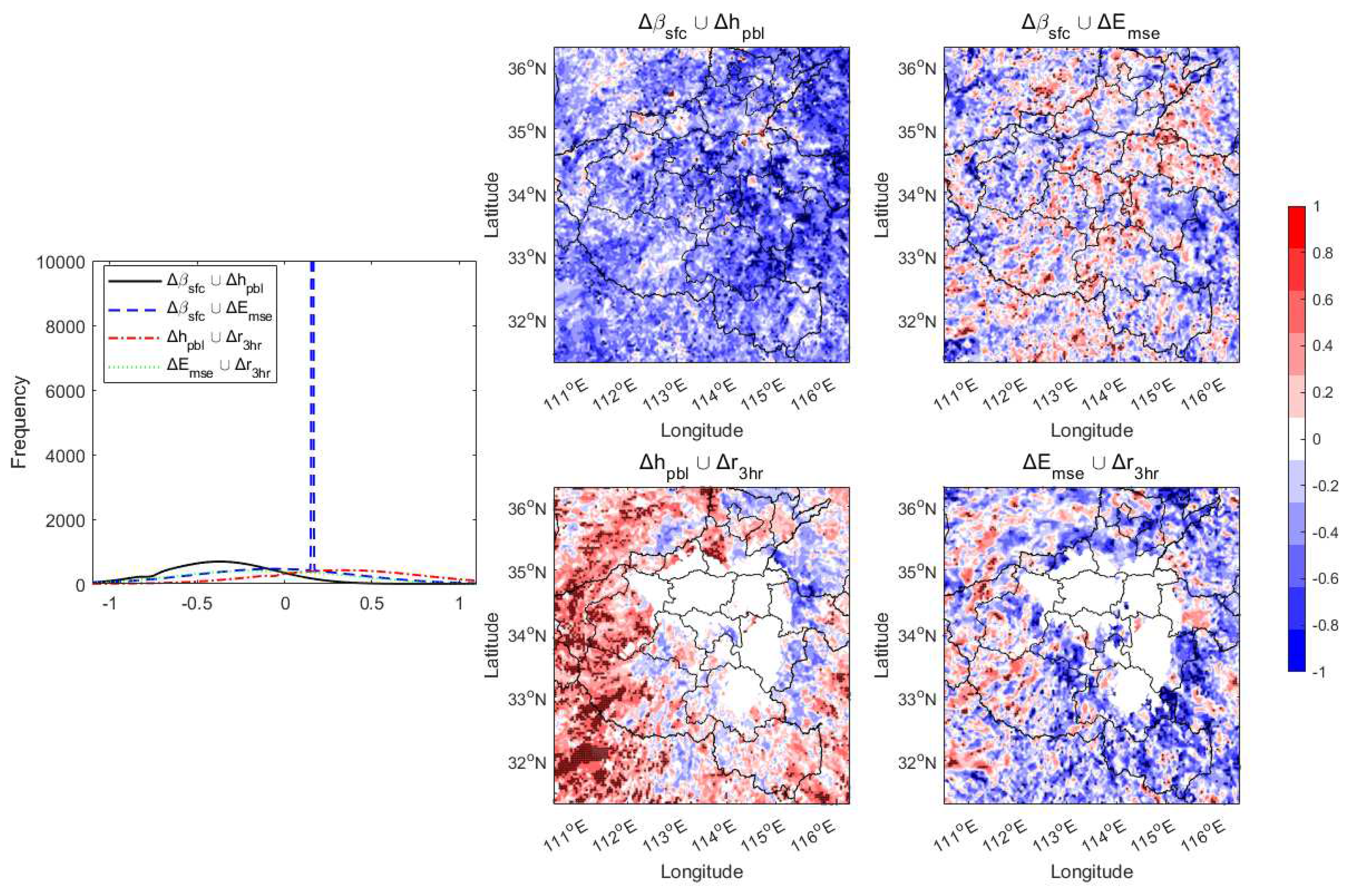
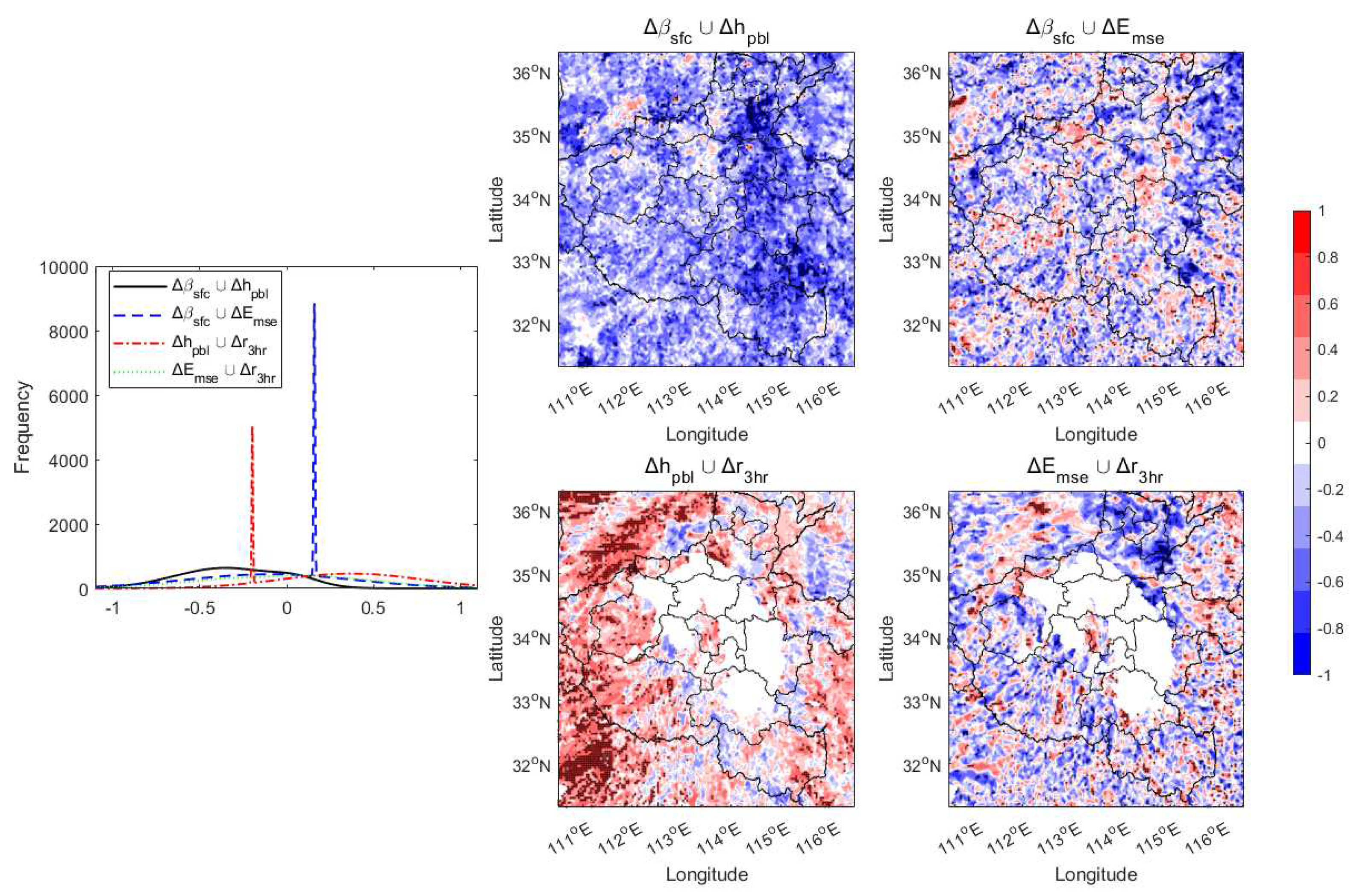
- Moist static energy () is more significant than PBL height () during the stepwise relation chains for both DP and WP. Deeper PBL with steeper surface flux slope in DP and shallower PBL with smoother surface flux slope in WP are significantly different. However, the point-wised relation chains interfaced by or are consistent for both DP and WP, while the relation intensity of DP is larger than WP. Nevertheless, the point-wised relation chains have been highly shaped by atmospheric forcing (e.g. environmental flows). This is especially pronounced for the chains characterized by relation intensity among surface flux, PBL height, and rainfall.
7. Discussion
Author Contributions
Funding
Institutional Review Board Statement
Informed Consent Statement
Data Availability Statement
Acknowledgments
Conflicts of Interest
References
- Betts, A.K. Land-surface-atmosphere coupling in observations and models. Journal of Advances in Modeling Earth Systems 2009, 1, 4. [Google Scholar] [CrossRef]
- Song, Y.M.; Guo, W.D.; Zhang, Y.C. Numerical study of impacts of soil moisture on the diurnal and seasonal cycles of sensible/latent heat fluxes over semi-arid region. Adv. Atmos. Sci. 2009, 26, 319–326. [Google Scholar] [CrossRef]
- Beljaars, A.; Viterbo, P.; Miller, M.; et al. The anomalous rainfall over the United States during July 1993: Sensitivity to land surface parameterization and SM anomalies. Mon. Wea. Rev. 1996, 124, 362–383. [Google Scholar] [CrossRef]
- Koster, R.D.; Suarez, M.J.; Higgins, R.W.; Van den Dool, H.M. Observational evidence that soil moisture variations affect precipitation, Geophys. Res. Lett. 2003, 30, 1241. [Google Scholar] [CrossRef]
- Liu, W.; Zhang, Q.; Li, C.; Xu, L.; Xiao, W. The influence of soil moisture on convective activity: a review. Theoretical and Applied Climatology 2022, 149, 221–232. [Google Scholar] [CrossRef]
- Koster, R.D.; Dirmeyer, P.A.; Guo, Z.; Bonan, G.; Chan, E.; Cox, P.; et al. Regions of Strong Coupling Between Soil Moisture and Precipitation. Science 2004, 305, 1138–1140. [Google Scholar] [CrossRef]
- Guillod, B.P.; Orlowsky, B.; Miralles, D.G.; Teuling, A.J.; Seneviratne, S. Reconciling spatial and temporal soil moisture effects on afternoon rainfall. Nat. Commun. 2015, 6, 6443. [Google Scholar] [CrossRef]
- Hsu, H.; Dirmeyer, P.A. Soil moisture-evaporation coupling shifts into new gears under increasing CO2. Nat. Commun. 2023, 14, 1162. [Google Scholar] [CrossRef] [PubMed]
- Zhang, R.; Xu, X.; Guo, J.; Sheng, Z. The ratio distribution of evapotranspiration to precipitation well related with soil thickness of Karst watershed in southwest China. J. Geophys. Res. Atmos. 2023, 128, e2022JD037951. [Google Scholar] [CrossRef]
- Divyansh, C.; Francina, D.; Christopher, M.T.; Cornelia, K.; Stephen, W.N. Dry-to-Wet Soil Gradients Enhance Convection and Rainfall over Subtropical South America. J. Hydrometeor. 2023. [CrossRef]
- Quintanar, A.; Mahmood, R.; Mofley, M.; et al. Lovanh, N. Simulation of boundary layer trajectory dispersion sensitivity to soil moisture conditions: MM5 and Noah-based investigation. Atmospheric Environment 2009, 43, 3774–3785. [Google Scholar]
- Suarez, A.; Mahmood, R.; Quintanar, A.; et al. A comparison of the MM5 and the RAMS simulations for land-atmosphere interactions under varying soil moisture. Tellus 2014, 66, 178–183. [Google Scholar]
- Mahmood, R.; Leeper, R.; Quintanar, A. Sensitivity of planetary boundary layer atmosphere to historical and future changes of land use/land cover, vegetation fraction, and soil moisture in Western Kentucky, USA. Global and Planetary Change 2011, 78, 36–53. [Google Scholar] [CrossRef]
- Leeper R, Mahmood R, and Quintanar, A. Influence of Karst Landscape on Planetary Boundary Layer Atmosphere: A Weather Research and Forecasting (WRF) Model-Based Investigation. J. Hydrometeor. 2011, 12, 1512–1529. [CrossRef]
- Simon, J.S., Bragg, A.D., Dirmeyer, P.A., and Chaney, N.W. Semi-coupling of a field-scale resolving land-surface model and WRF-LES to investigate the influence of land-surface heterogeneity on cloud development. Journal of Advances in Modeling Earth Systems 2021, 13, e2021MS002602. [CrossRef]
- Santanello, J.A., Lawston, P., Kumar, S.V.; et al. Understanding the impacts of soil moisture initial conditions on NWP in the context of land–atmosphere coupling. J. Hydrometeor 2019, 20, 793–819. [CrossRef]
- Findell, K.L.; Eltahir, E.A.B. Atmospheric controls on soil moisture-boundary layer interactions. Part I: framework developmen. J. Hydrometeor. 2003, 4, 552–569. [Google Scholar] [CrossRef]
- Findell, K.L.; Eltahir, E.A.B. Atmospheric Controls on Soil Moisture–Boundary Layer Interactions. Part II: Feedbacks within the Continental United States. J. Hydrometeor. 2003, 4, 570–583. [Google Scholar] [CrossRef]
- Ek, M.; Mahrt, L. Daytime evolution of relative humidity at the boundary-layer top. Mon. Wea. Rev. 1994, 122, 2709–2721. [Google Scholar] [CrossRef]
- Ek, M. B.; Holtslag, A. A. M. Influence of soil moisture on boundary cloud development. J. Hydrometeor. 2004, 5, 86–99. [Google Scholar] [CrossRef]
- Tawfik, A.B.; Dirmeyer, P.A. A process-based framework for quantifying the atmospheric preconditioning of surface-triggered convection. Geophys. Res. Lett. 2014, 41, 173–178. [Google Scholar] [CrossRef]
- Tawfik, A.B., Dirmeyer, P.A., and Santanello, J.A. The heated condensation framework. part i: description and southern great plains case study. J. Hydrometeor. 2015, 16, 150603105509002.
- Tawfik, A.B., Dirmeyer, P.A., and Santanello, J.A. The heated condensation framework. part ii: climatological behavior of convective initiation and land-atmosphere coupling over the conterminous united states. J. Hydrometeor. 2015, 16, 150603105509002.
- Santanello, J.A., Peters-Lidard, C.D., and Kumar, S. A modeling and observational framework for diagnosing local land–atmosphere coupling on diurnal time scales. J. Hydrometeor. 2009, 10, 577–599. [CrossRef]
- Delworth, T.L.; Manabe, S. The influence of potential evaporation on the variabilities of simulated soil wetness and climate. J. Climate 1988, 1, 523–547. [Google Scholar] [CrossRef]
- Delworth, T.L.; Manabe, S. The influence of soil wetness on near-surface atmospheric variability. J. Climate 1989, 2, 1447–1462. [Google Scholar] [CrossRef]
- Dirmeyer, P.A. The terrestrial segment of soil moisture–climate coupling. Geophys. Res. Lett. 2011, 38, L16702. [Google Scholar] [CrossRef]
- Guo, Z.C., Dirmeyer, P.A., Bonan, G., Chan, E., Cox, P.; et al. GLACE: The Global Land–Atmosphere Coupling Experiment. Part II: Analysis. J. Hydrometeor., 2006, 7, 611–625. [CrossRef]
- Santanello, J.A., Dirmeyer, P.A., Ferguson, C.R.; et al. Land–atmosphere interactions: the LoCo perspective. BAMS, 2018, (6). et al. Land–atmosphere interactions: the LoCo perspective. BAMS, 2018.
- Sun, G.; Hu, Z.; Ma, Y.; Xie, Z.; Yang, S.; Wang, J. Analysis of local land-atmosphere coupling in rainy season over a typical underlying surface in Tibetan Plateau based on field measurements and ERA5. Atmospheric Research 2020, 243105025. [Google Scholar] [CrossRef]
- Sun, G., Hu, Z., Ma, Y., Xie, Z., and Yang, S. Simulation analysis of local land-atmosphere coupling in rainy season over a typical underlying surface in Tibetan Plateau. Hydrology and Earth System Sciences 2020, 24, 5937–5951. [CrossRef]
- Abdolghafoorian, A., and Dirmeyer, P.A. Validating the land-atmosphere coupling behavior in weather and climate models using observationally based global products. J. Hydrometeor. 2021, 22, 1507–1523.
- Zhao, C., Meng, X., Li, Y., Lyu, S., Guo, J., & Liu, H. Impact of soil moisture on afternoon convection triggering over the Tibetan Plateau based on 1-D boundary layer model. J. Geophys. Res. Atmos. 2022, 127, e2021JD035591.
- Quintanar, A.; Mahmood, R. Ensemble forecast spread induced by soil moisture changes over mid-south and neighbouring mid-western region of the USA. Tellus 2012, 64, 145–153. [Google Scholar] [CrossRef]
- Min, J.Z., Guo, Y.K., and Wang, G.J. Impacts of soil moisture on typical frontal rainstorm in yangtze river basin. Atmosphere 2016, 7, 42. [CrossRef]
- Xue, M. Preface to the Special Collection on the July 2021 Zhengzhou, Henan Extreme Rainfall Event. Adv. Atmos. Sci. 2023, 40, 335–336. [Google Scholar] [CrossRef]
- Luo, Y., Zhang, J., Yu, M.; et al. On the Influences of Urbanization on the Extreme Rainfall over Zhengzhou on 20 July 2021: A Convection-Permitting Ensemble Modeling Study. Adv. Atmos. Sci. 2023, 40, 393–409. [CrossRef]
- Tewari, M., F. Chen, W. Wang, J. Dudhia, M.A. LeMone, K. Mitchell, M. Ek, G. Gayno, J. Wegiel, and R. H. Cuenca, 2004: Implementation and verification of the unified NOAH land surface model in the WRF model. 20th conference on weather analysis and forecasting/16th conference on numerical weather prediction, pp. 11–15.
- Skamarock, W.C., Klemp, J.B., Dudhia, J., Gill, D.O., Barker, D., Duda, M.G., … Powers, J.G. A Description of the Advanced Research WRF Version 3 (No. NCAR/TN-475+STR). University Corporation for Atmospheric Research. 2008.
- Thompson, Gregory, Paul, R. Field, Roy M. Rasmussen, William D. Hall. Explicit Forecasts of Winter Precipitation Using an Improved Bulk Microphysics Scheme. Part II: Implementation of a New Snow Parameterization. Mon. Wea. Rev. 2008, 136, 5095–5115. [CrossRef]
- Iacono, M.J., J.S. Delamere, E.J. Mlawer, M.W. Shephard, S.A. Clough, and W. D. Collins. Radiative forcing by long–lived greenhouse gases: Calculations with the AER radiative transfer models. J. Geophys. Res. Atmos. 2008, 113, D13103. [CrossRef]
- Kain, J.S. The Kain–Fritsch convective parameterization: An update. J. Appl. Meteor. 2004, 43, 170–181. [Google Scholar] [CrossRef]
- Jimenez, Pedro A., Jimy Dudhia, J. Fidel Gonzalez–Rouco, Jorge Navarro, Juan P. Montavez, and Elena Garcia–Bustamante. A revised scheme for the WRF surface layer formulation. Mon. Wea. Rev. 2012, 140, 898–918.
- Hong, Song–You, Yign Noh, Jimy Dudhia. A new vertical diffusion package with an explicit treatment of entrainment processes. Mon. Wea. Rev. 2006, 134, 2318–2341. [CrossRef]
- Andras H, Paul B, Gionata B, et al. The impact of observations in the ECMWF latest reanalysis system: WMO workshop, Shanghai, 10-13 May 2016. 13 May.
- Wang, M.Y., Yao, S., Jiang, L.P., Liu, Z.Q., Shi, C.X., Hu, K.X., Zhang, T., Zhang, Z.S., Liu, J.W. Collection and Pre-Processing of Satellite Remote-Sensing Data in CRA-40 (CMA’s Global Atmospheric ReAnalysis). Advances in Meteorological Science and Technology (In Chinese). 2018, 8, 158–163.
- Beaudoing, H. and M. Rodell, NASA/GSFC/HSL (2020), GLDAS Noah Land Surface Model L4 3 hourly 0.25 x 0.25 degree V2.1, Greenbelt, Maryland, USA, Goddard Earth Sciences Data and Information Services Center (GES DISC), Accessed: [Data Access Date].
- Sun, S.; Shi, C.; Pan, Y.; et al. Applicability assessment of the 1998-2018 CLDAS multi-source precipitation fusion dataset over China. Journal of Meteorological Research 2020, 34, 879–892. [Google Scholar] [CrossRef]
- Fieller, E.C., Hartley, H.O., and Pearson, E.S. Tests for rank correlation coefficients. I. Biometrika 1957, 44, 470–481. [CrossRef]
- Shen, F., Min, J., and Xu, D. Assimilation of radar radial velocity data with the WRF Hybrid ETKF–3DVAR system for the prediction of Hurricane Ike (2008). Atmospheric Research 2016, 169, 127–138. [CrossRef]
- Shen, F., Xu, D., Min, J., Chu, Z., and Li, X. Assimilation of radar radial velocity data with the WRF hybrid 4DEnVar system for the prediction of hurricane Ike (2008). Atmospheric Research 2020, 234, 104771. [CrossRef]
- Xu, D., Liu, Z., Huang, X. Y., Min, J., and Wang, H. Impact of assimilating IASI radiance observations on forecasts of two tropical cyclones. Meteorology and Atmospheric Physics 2013, 122, 1–18. [CrossRef]
- Shen, F.; Min, J. Assimilating AMSU-A radiance data with the WRF Hybrid En3DVAR system for track predictions of Typhoon Megi (2010). Advances in Atmospheric Sciences 2015, 32, 1231–1243. [Google Scholar] [CrossRef]
- Xu, D., Min, J., Shen, F., Ban, J., and Chen, P. Assimilation of MWHS radiance data from the FY-3B satellite with the WRF Hybrid-3DVAR system for the forecasting of binary typhoons. Journal of Advances in Modeling Earth Systems 2016, 8, 1014–1028. [CrossRef]
- Xu, D., Liu, Z., Fan, S., Chen, M., and Shen, F. Assimilating all-sky infrared radiances from Himawari-8 using the 3DVar method for the prediction of a severe storm over North China. Advances in Atmospheric Sciences 2021, 38, 661–676. [CrossRef]
- Xu, D.; Zhang, X.; Liu, Z.; Shen, F. All-sky infrared radiance data assimilation of FY-4A AGRI with different physical parameterizations for the prediction of an extremely heavy rainfall event. Atmospheric Research 2023, 106898. [Google Scholar] [CrossRef]
- Shen, F., Xu, D., Li, H., Min, J., and Liu, R. Assimilation of GPM Microwave Imager Radiance data with the WRF hybrid 3DEnVar system for the prediction of Typhoon Chan-hom (2015). Atmospheric Research 2021, 251, 105422. [CrossRef]
- Song, L. Song, L., Shen, F., Shao, C., Shu, A., and Zhu, L. Impacts of 3DEnVar-Based FY-3D MWHS-2 Radiance Assimilation on Numerical Simulations of Landfalling Typhoon Ampil (2018. Remote Sens. 2022, 14, 6037. [Google Scholar] [CrossRef]
- Zhang, X.; Xu, D.; Liu, R.; Shen, F. Impacts of FY-4A AGRI Radiance Data Assimilation on the Forecast of the Super Typhoon “In-Fa” (2021). Remote Sens. 2022, 14, 4718. [Google Scholar] [CrossRef]
- Shu, A.; Shen, F.; Jiang, L.; Zhang, T.; Xu, D. Assimilation of Clear-sky FY-4A AGRI radiances within the WRFDA system for the prediction of a landfalling Typhoon Hagupit (2020). Atmospheric Research 2022, 283. [Google Scholar] [CrossRef]
- Liu, Y.; Yang, Y. Spatial-temporal variability pattern of multi-depth soil moisture jointly driven by climatic and human factors in China. Journal of Hydrology 2023, 619, 129313. [Google Scholar] [CrossRef]
Disclaimer/Publisher’s Note: The statements, opinions and data contained in all publications are solely those of the individual author(s) and contributor(s) and not of MDPI and/or the editor(s). MDPI and/or the editor(s) disclaim responsibility for any injury to people or property resulting from any ideas, methods, instructions or products referred to in the content. |
© 2023 by the authors. Licensee MDPI, Basel, Switzerland. This article is an open access article distributed under the terms and conditions of the Creative Commons Attribution (CC BY) license (http://creativecommons.org/licenses/by/4.0/).


