1. Introduction
The magnetic characteristics of mixed-spin systems have recently attracted both theoretical and experimental attention [
1,
2,
3]. These systems are especially well suited for studying the magnetic properties of a particular class of magnetic materials, in addition to some technical applications [
4]. Therefore, mixed-spin Ising models have been extensively studied in the literature lately [
5]. In Ref. [
6], on the Cayley tree we classified the disordered phases corresponding to the Ising model with spin-1 and spin 1/2. Then, on the second-order Cayley tree, we examined the phase transition problem of the Ising model with spin-2 and spin 1/2 and discussed the chaotic behavior of the corresponding dynamical system [
7]. The main methods for examining some properties of Ising models with the mixed spin on the square lattice [
5], Bethe lattice [
8] and Cayley tree [
6,
7] are Monte Carlo simulations [
5], the cavity method [
9,
10,
11], the Kolmogorov consistency method [
6,
7], the iteration method, and transfer matrix method. In [
12], the magneto thermal parameters that characterize the magnetocaloric effect (MCE) behaviors, such as entropy, entropy change, and adiabatic cooling rate, are precisely calculated using the transfer matrix approach.
There are several approaches in the literature to figure out the free energy of the specified model. The free energy of the lattice models on the Bethe lattice was calculated while boundary conditions were taken into consideration [
8,
13,
14,
15,
16]. In-depth research has been done on the thermodynamic properties of the 1D Ising model with single spin-
s by means of the transfer matrix [
17,
18,
19].
I am not aware of any research into the thermodynamic properties of 1D Ising models with mixed spin. In this brief essay, we will use the transfer matrix approach to determine the thermodynamic variables related to 1D-MSIM with the mixed spin-.
Due to its widespread general application across numerous physical models, the transfer matrix approach is the most extensive technique. In [
18], the transfer matrix approach is used to conduct an analytical study of the 1D Ising model with spin-
s. In order to grasp physical issues as well as statistical mechanics, it is essential to compute thermodynamic quantities like free energy, entropy, magnetization, and magnetic susceptibility [
19]. In this present paper, we enlarge a specific bond and establish the transfer matrix that corresponds to the bond from site
j to site
. By using the trace of several transfer matrices multiplied simultaneously, we reconstruct the partition function
Z.
In this short study, inspired by the results given for 1D Ising model with the single spin-
s [
18], we will first calculate the partition function and then the free energy of 1D-MSIM with mixed spin-
having the nearest neighbor interactions and external field by means of the transfer matrix. To calculate the model’s free energy, entropy, magnetization, and susceptibility, we establish some exact formulas via the corresponding transfer matrix. We study the phase transition issue by using the cavity approach to the corresponding iterative equations of the model. We estimate the periodicity of the model numerically.
2. Preliminaries
Here, we will review definitions and key findings in the construction of the partition function for the 1D-MSIM with mixed spin- on the one-dimensional lattice . We denote the set of integers by and the set of strictly positive integers by . Two vertices x and y, are called nearest-neighbor (NN) if there exists an edge connecting them, which is denoted by . For , the distance is the length (the number of edges) of the shortest path connecting x with y. For any , the direct successor of the vertex x is defined by
Denote the set of even natural numbers by
and the set of odd natural numbers by
. We will consider the mixed spin state spaces denoted by
and
. For
, a spin configuration
on
A is defined as a function
Let us consider finite set
. Let
and
be the spaces of infinite configurations and
and
be the spaces of finite configurations.
represents the configuration space. Elements of
will be denoted by
, for
. Similarly, elements of
will be denoted by
, for
In this paper, the spins in
and
can be placed on the odd-numbered vertices and the even-numbered vertices, respectively, when mixed spins are designed on the lattice
(see
Figure 1).
2.1. Construction of the Partition Function Associated with the Model
Let us construct the partition function corresponding to 1D-MSIM with mixed spin on the lattice .
Let
, so one has
where
and
.
Fix a finite volume
. Let
be the set of nearest-neighbor edges with at least one endpoint in
. We will examine in detail the 1D-MSIM with mixed spin
built on the lattice
, having Hamiltonian
where the energy of each link tying up nearby sites is represented by the first sum, and the energy of each site is represented by the second sum.
The partial partition functions associated with the Hamiltonian (
1) can be found as follows:
where
,
and
J is the coupling constant.
Given the finite set
, by containing the boundary spins, or the spins on the
-th level, we can construct the summation of equation (
2). Consequently, we state that the density-free energy function is
where
is the total partition function.
As a result of derivatives of the free energy function with respect to certain parameters, many authors have studied other thermodynamic properties [
18,
19].
If the largest eigenvalue of the transfer matrix corresponding to the given model is , the thermodynamic quantities of this system are obtained as follows:
3. Construction of the Partition Function of the Model via Transfer
Matrices
The Kramers-Wannier transfer technique may be used to construct the partition function. This method requires building a transfer matrix and determining its eigenvalues.
3.1. Partition Function and the Boltzmann Weight
It is well-known that the total partition function
depends on the particular realization
. It is common knowledge that the total partition function equals the Boltzmann weight’s sum over all possible states. Here we will consider blocks or configurations of length
and under zero boundary condition. If we want to rewrite the Hamiltonian (
1) for all configurations on the configuration space
, we can get the Boltzmann weight in the form:
From (
1), for
we will denote the energy of the bond between sequential vertices
and
by
Similarly, for
we will denote the energy of the bond between sequential vertices
and
by
It is common knowledge that the partition function equals the sum of the Boltzmann weight
over all possible states in the lattice
[
18,
19]. Therefore, for the configuration
we can write the Boltzmann weight
in the form
For this system, the canonical partition function can be written as
The next step is to decompose the bonds using the bond representation and factor the Boltzmann weights into pairwise factors.
3.2. The Transfer Matrices
Here we will construct the transfer matrices corresponding to 1D-MSIM with the
mixed spin on the lattice
. We will get two different transfer matrices. First, let us place the spins of the set
on the odd-numbered vertices of the lattice
, and the spins in the set
on the even-numbered vertices. So, we define the entries of the transfer matrix
as follows:
where
and
for
.
So, similarly, we can define the entries of the transfer matrix
by
where
and
for
.
From (
10), (
12) and (
13), we get
One can easily see that matrix
has Card
Card
dimensional while matrix
has Card
Card
dimensional. Assume that
. The total partition function can be written as the trace of the product of
random transfer matrices.
3.3. 1D-MSIM with Mixed Spin-
Due to the difficulty of computation of the transfer matrix and its eigenvalues for and , we will restrict ourselves to the mixed spin . In this subsection, we will compute the thermodynamic quantities of 1D-MSIM with mixed spin . So we consider the mixed spins as and .
Firstly, we define the transfer matrix as
, for
and
. So we have
Secondly, let us place the spins of the set
on the even-numbered vertices of the lattice
, and the spins in the set
on the odd-numbered vertices (see Fig.
Figure 1). We define the second transfer matrix as
, for
and
. Thus, we obtain
3.4. Translation-Invariant
We will assume
for all
and
. This property is called the translation-invariant property. Thus, the transfer matrices
and
given in (
15) and (
16) are obtained as follows
Case I
If we multiply the transfer matrices
and
given in (
17) and (
18) we get the following square transfer matrix
After some tedious and complicated algebraic processes, the eigenvalues of the matrix
is obtained as follows:
where
Substitute the variables
and
for the sake of simplicity. Following, we have
By computing the trace of the matrix product, we can determines the partition function as
where
denotes the eigenvalue of the transfer matrix
for
From (
11), we get
where
denote the eigenvalues of transfer matrix
.
So, one has
for
. As is well known, the model’s critical behavior manifests itself in the thermodynamic limit
, therefore the largest eigenvalue
of transfer-matrix given in (
19) stands as the only indicator of the bulk free energy:
3.5. Behavior of the thermodynamic quantities of 1D-MSIM with mixed spin- in absence of magnetic
field
For
, we obtain the transfer matrix
given in (
19) as
We get the set of eigenvalues of the matrix
is obtained as follows:
It is clear that
From the formula given in (
23), we get
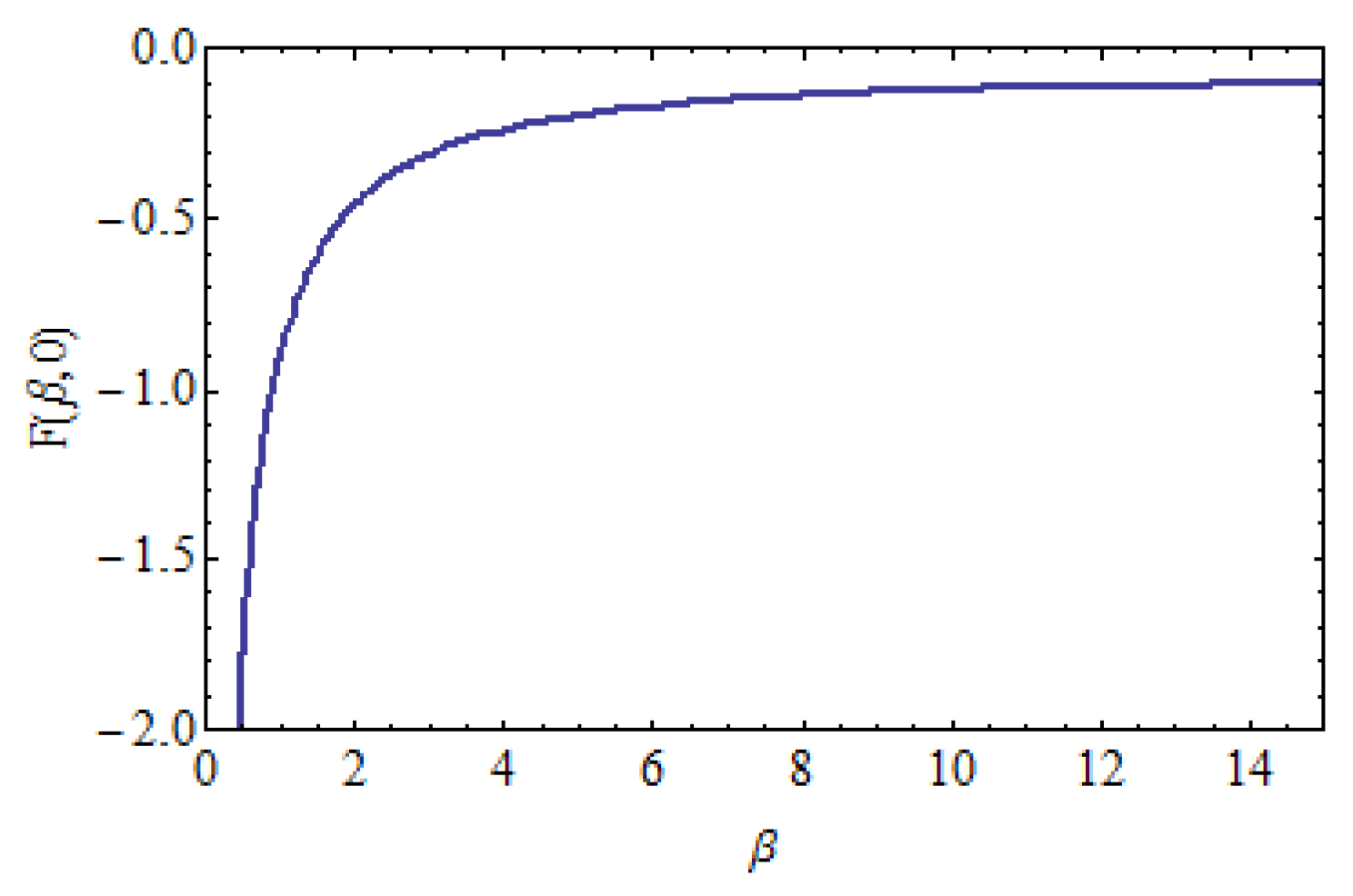
Figure 2 shows the graph of free energy
given in (
25) as a function of
for
. From
Figure 2 it can be seen that the free energy is approaching zero for
.
In case of the disappearance of the external magnetic field, from (
5) we obtain the entropy of the model as
Similarly, from (
6) we get the internal energy as
The changes in the entropy of 1D-MSIM with mixed spin
are given in
Figure 3. Results show that the internal energy converges to zero at the higher temperature values, while becoming constant 0 as
. When the temperature increases, the entropy increases until reaches to
and goes to zero at low temperatures.
Case II
Note that while successively placing spins on the vertices of a one-dimensional lattice, if the elements of
are placed first vertex of the lattice
, then a transfer matrix having
dimensional is obtained, and the eigenvalues of the transfer matrix are the same as those of the previous matrix
.
If we substitute the variables
and
for simplicity’s sake. We get
We obtain the set of eigenvalues of the matrix
given in
as
It should be noted here that the eigenvalues of the matrices
and
are the same, except for 0. Therefore, it was obtained as
(see equations (
20) and (
30)). Therefore, we can choose any spin on the starting vertex, while mixed spins are placed on consecutive vertices of the lattice. From (
20) and (
30), it is clear that
.
3.6. Magnetization and Magnetic Susceptibility
In this subsection, we will construct magnetization and magnetic susceptibility by means of the eigenvalue
in the formula (
30).
Let us consider the reduced nearest neighbor spin-spin coupling interactions and the reduced magnetic field , we have
magnetization
and susceptibility
We will not give the exact expressions of the formulas for the magnetization and susceptibility quantities here, because the operations are excessively long and complex. We will numerically examine the behavior of these two quantities as functions of h and T.
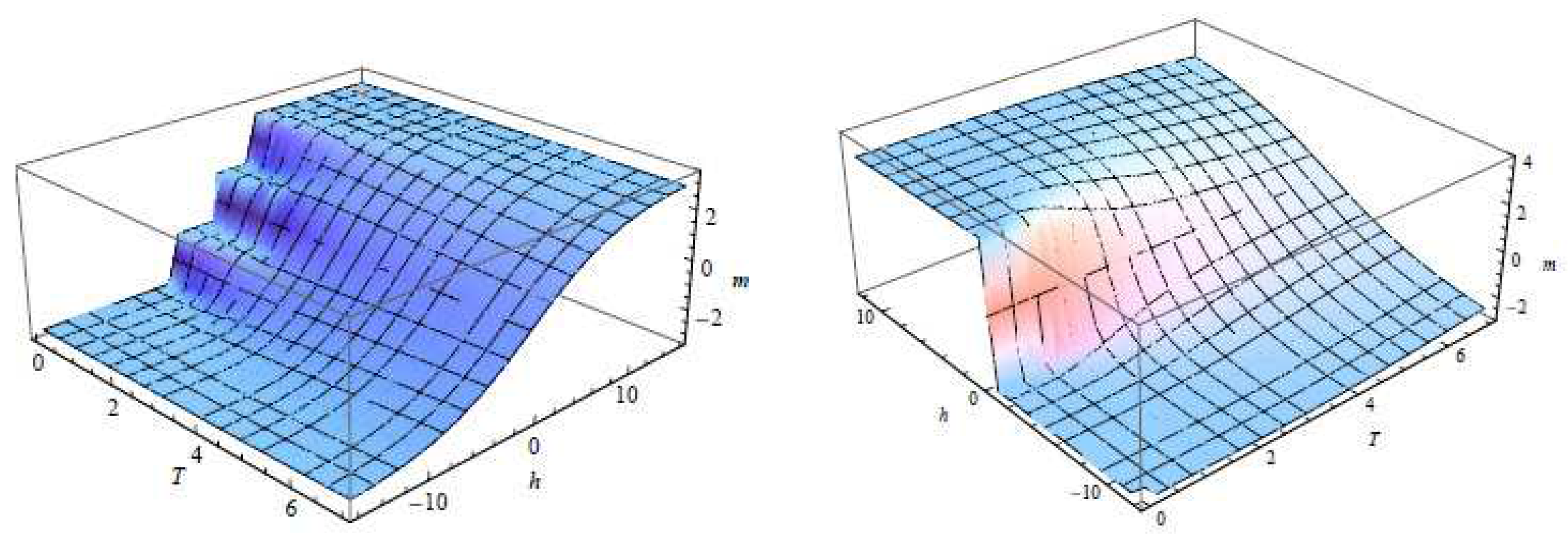
The behavior of the magnetization function described in the Equation (
31) is illustrated in
Figure 4. We have used the Mathematica [
20] to plot these figures, taking into account the eigenvalue
in the Formula (
30). For
, as the temperature
T increases, the smoothness of the function decreases and exhibits a behavior similar to the step function. On the other hand, for
, the surface of the function becomes smooth.
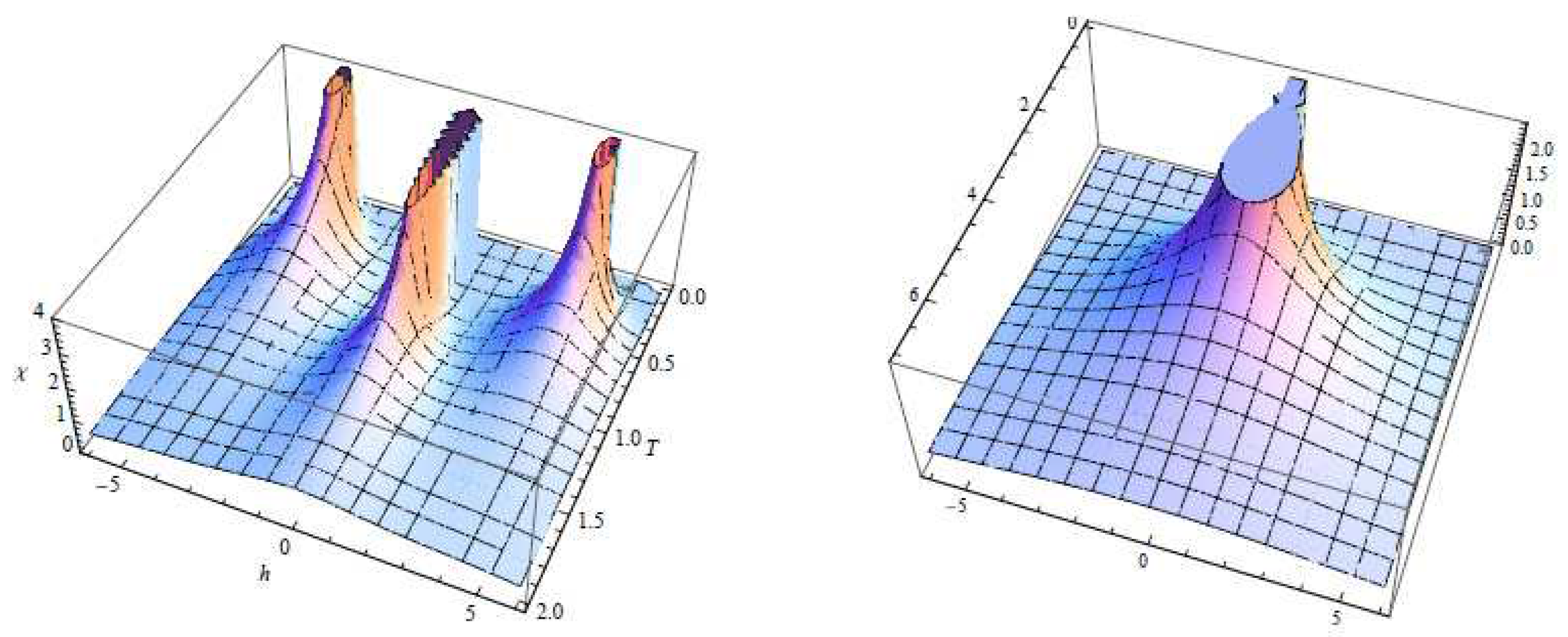
Figure 5 show the behavior of the susceptibility function given in equation (
32). For
, three stacks resembling a boot are observed, a stack appears for
in the chosen region
,
.
4. Nonexistence Phase Transition in the Absence of the External Magnetic Field
In this section, we will study 1D-MSIM with the mixed spin-(1,1/2) by means of the ERR.
Suppose that
,
and
, from equations (
43) and (44) we get
where
.
If we assume
,
and
, then we obtain a new three-dimensional rational dynamical system (3D-RDS) as
If the values of
x and
y in equations (37) and (38) are substituted in equation (
36), one gets the following rational recursive equation
:
From (
39), we get a second-order equation
From equation (
40), it is clear that the function
f given in (
39) has only one positive fixed point, so there is no phase transition for the given model.
The graphs of the function
f for antiferromagnetic (
) and ferromagnetic (
) values are shown in
Figure 6. The diagrams show that the function in both cases has just two fixed points. Additionally, there is only one positive fixed point. As a result, there is just one Gibbs measure and no phase transition in the model. As is well known, the classical single spin 1D Ising model’s phase transition issue has attracted the interest of statistical mechanics researchers for over a century, and it has been established that there is no phase transition [
21]. In this present paper, we have demonstrated the mixed spin 1D Ising model’s absence of a phase transition as an example.
4.1. Chaoticity of the Model
It has long been challenged whether a model’s phase transition and the chaotic behavior of the corresponding dynamical system are related. In this subsection, we will investigate the chaoticity of the 3D-RDS given in (
36)-(38). With the help of the Lyapunov exponent, we will numerically study the model’s chaotic behavior.
From the definition of the Lyapunov exponent, we get
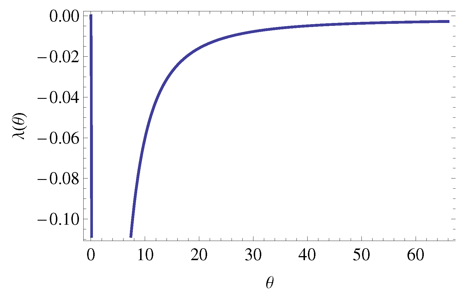
Figure 7 shows the Lyapunov exponent of the dynamical system corresponding to the 1D-MSIM with mixed spin-(1,1/2). It is seen that the Lyapunov exponent is always negative in the ferromagnetic region. Therefore, the rational function
given in (
39) is periodic. The behavior of the Lyapunov exponent
in the antiferromagnetic region can also be examined.
5. The Average Magnetization for Mixed Spin-(1,1/2)
In this section, by using the exact recursion relations (ERR) (see [
4]), we will get the partial partition functions of the 1D-MSIM with mixed spin-
. Contrary to the previous sections, here we will place the spins of
in the first vertex of the lattice and the spins of
in the second vertex of the lattice, while placing spins at the vertices of the lattice
, so for
, we will get
and
. With the help of the cavity method [
9,
10,
11], we obtain the partial partition functions as follows:
5.1. The Average Magnetization
In this subsection, assuming there is an external magnetic field, we obtain the magnetization equations for spins
s and
, respectively, as follows.
We are only concerned with magnetization for the mixed spin-(1,1/2) here, since the operations for obtaining partition functions are excessively long. So, from (
45) and (
46), we get
The following equation results from the simple substitutions of the variables
and
Now let us assume the external magnetic field
h (
) is zero. In this case, after some calculations as in Ref. [
9], we can show that the fixed point for the 3D-RDS given in (
36)-(38) is only
and
. So, we get zero average magnetization around this fixed point. That is, we have
6. Conclusions
As is known, there are many methods for calculating the free energy of lattice models on Bethe lattices. Some of these are the exact recursion relations [
4], the cavity method [
13,
14], and vector-valued boundary conditions [
15]. One of the most widely used methods to examine thermodynamic quantities corresponding to a 1D Ising model is the transfer matrix technique [
18,
19]. In this present work, we have constructed the partial partition functions associated with 1D-MSIM having mixed spin-
using the transfer matrix. We have computed some thermodynamic quantities such as the free energy, entropy, magnetization, and susceptibility of the model. To my knowledge, the thermodynamic properties of the single spin 1D Ising model have been studied in a number of studies so far. Using the transfer matrix method, we have evaluated the thermodynamic features of the 1D-MSIM for the first time. For the single spin-Isign model, Amin et al. [
18] plotted the magnetization and susceptibility in two dimensions. The findings obtained in our present article show different behaviors. Frankly, we cannot comment on the physical meaning of such behavior. We think our findings will be of interest to physicists.
In our previous studies, we proved that there is a phase transition for the mixed spin Ising model on the Cayley tree using many methods [
6,
7,
9]. As it is known, there is no phase transition for a single spin 1D Ising model [
21]. In this study, we have investigated how mixed spins affect thermodynamic quantities and the existence of phase transition. We have demonstrated the uniqueness of limiting Gibbs measures associated with 1D-MSIM having mixed spin-(1,1/2). We showed that if the external magnetic field is zero, for the aforementioned model, there is no phase transition. These topics are covered in introductory courses in statistical mechanics at the undergraduate level. We believe that the results of our present study will be of interest to a wide readership of statistical mechanics. Our next research will deal with these issues. We will analyze the isothermal entropy change of the average magnetization for 1D-MSIM considering the approach given by Albayrak [
4].
Acknowledgments
The author would like to thank the Simons Foundation (10.13039/100000893) and the Institute of International Education. This work was mostly completed while I was working as a visiting scientist at ICTP. Therefore, the author thanks ICTP for their hospitality.
References
- De La Espriella N., Arenas A. J., Paez Meza M.S., Critical and compensation points of a mixed spin-2-spin-5/2 Ising ferrimagnetic system with crystal field and nearest and next-nearest neighbors interactions, J. Magn. Magn. Mater., 417, 434-441 (2016). [CrossRef]
- De La Espriella, N., Buendia G.M., Madera J.C., Mixed spin-1 and spin-2 Ising model: study of the ground states, J. Phys. Commun., 2, 025006 (2018). [CrossRef]
- Kaneyoshi T., Phase transition of the mixed spin system with a random crystal field, Physica A, 153, 556-566 (1988). [CrossRef]
- Albayrak E., The study of mixed spin-1 and spin-1/2: Entropy and isothermal entropy change, Physica A, 559, 125079 (2020). [CrossRef]
- De La Espriella, N., Buendia G.M., Magnetic behavior of a mixed Ising 3/2 and 5/2 spin model, J. Phys.: Condens. Matter 23 (2011) 176003 (7pp). [CrossRef]
- Akın H., Mukhamedov F., Phase transition for the Ising model with mixed spins on a Cayley tree, J. Stat. Mech. (2022) 053204. [CrossRef]
- Akın H., The classification of disordered phases of mixed spin (2,1/2) Ising model and the chaoticity of the corresponding dynamical system, Chaos, Solitons & Fractals, 167, 2023, 113086. [CrossRef]
- Seino M., The free energy of the random Ising model on the Bethe lattice, Physica A, 181 (3-4), 233-242 (1992). [CrossRef]
- Akın H., Quantitative behavior of (1,1/2)-MSIM on a Cayley tree, Chinese Journal of Physics 2023; 83:501-514. [CrossRef]
- Ostilli M., Cayley Trees and Bethe Lattices: A concise analysis for mathematicians and physicists, Physica A 391 (2012) 3417–3423. [CrossRef]
- Mézard M., Parisi G., The Bethe lattice spin glass revisited, Eur. Phys. J. B 20 (2001) 217–233. [CrossRef]
- Qi Y., Liu J., Yu N.-S., Du A., Magnetocaloric effect in ferroelectric Ising chain magnet, Solid State Commun. 233 (2016) 1–5. [CrossRef]
- Akın H., A novel computational method of the free energy for an Ising model on Cayley tree of order three, Chin. J. Phys., 77, 2276-2287 (2022). [CrossRef]
- Akın H., Calculation of the free energy of the Ising model on a Cayley tree via the self-similarity method, Axioms, 2022, 11 (12), 703. [CrossRef]
- Mukhamedov F., Akın H. and Khakimov O., Gibbs measures and free energies of the Ising-Vannimenus Model on the Cayley tree, J. Stat. Mech., 2017 (053101-059701) 053208. [CrossRef]
- Akın H., Ulusoy S., A new approach to studying the thermodynamic properties of the q-state Potts model on a Cayley tree, Chaos, Solitons & Fractals, 174, 2023, 113811. [CrossRef]
- Salinas, S.R.A., Phase Transitions and Critical Phenomena: Classical Theories. In: Introduction to Statistical Physics. Graduate Texts in Contemporary Physics. Springer, New York, NY (2001).
- Amin M. E., Mubark M., and Amin Y., On the critical behavior of the spin-s ising model, Revista Mexicana de Fisica, 69, 021701 1–6 (2023). [CrossRef]
- Wang W., Diaz-Mendez R. and Capdevila R., Solving the one-dimensional Ising chain via mathematical induction: an intuitive approach to the transfer matrix, Eur. J. Phys., 40 (6) 065102 (2019). [CrossRef]
- Wolfram Research, Inc., Mathematica, Version 8.0, Champaign, IL (2010).
- Ising E., Beitrag zur theorie des ferromagnetismus, Z. Physik 31 (1925) 253.
|
Disclaimer/Publisher’s Note: The statements, opinions and data contained in all publications are solely those of the individual author(s) and contributor(s) and not of MDPI and/or the editor(s). MDPI and/or the editor(s) disclaim responsibility for any injury to people or property resulting from any ideas, methods, instructions or products referred to in the content. |
© 2023 by the authors. Licensee MDPI, Basel, Switzerland. This article is an open access article distributed under the terms and conditions of the Creative Commons Attribution (CC BY) license (http://creativecommons.org/licenses/by/4.0/).


