1. Introduction
According to World Health Organization (WHO), diabetes is one of the world’s largest causes of premature deaths. WHO estimates, in 2014, that exist 422 million adults with diabetes worldwide [
1]. Findings of the International Diabetes Federation (IDF) estimate that 537 million people have diabetes, and this number is projected to reach 643 million by 2030, and 783 million by 2045. In Brazil in 2021, an estimated 15.7 million people were living with diabetes. This estimate positions the country in sixth place globally, and first place in Latin America. This number is expected to grow in the next 20–30 years [
2]. Diabetes standards of care, established by WHO, recommend that self-monitoring with glucose meter technologies are essential strategies for managing their condition [
3]. A common characteristic of all types of diabetes, monitored by glucose meters, is hyperglycemia which can lead to the development of long-term complications when left untreated. Thus, poor control accelerates its progression, and to prevent complications, their management is crucial to improve glycemic control.
During the past decade, Continuous Glucose Monitoring Devices (CGMDs) have transformed patient diabetes management. They are small and easy to use, equipped with connectivity to other devices and the cloud, have digital management tools for data analysis, require small blood sample volumes, and provide measurement results within seconds for management decisions. With the improved analytical performance of these CGMDs, self-monitoring is no longer the only option for glucose monitoring, and in-depth analysis of the collected data with Artificial Intelligence (AI) approaches can allow the creation of additional insights [
4].
Some literature studies address AI as a form to influence diabetes patients’ self-management and facilitate interactions with health professionals and the healthcare system. One example of this is the systematic review of [
5], which presents the advancements in the field of diabetes management using continuous monitoring smart devices in combination with AI techniques such as support vector regression (SVR), random forest (RF), k-nearest neighbors (KNN), and artificial neural networks (ANN) for regression tasks.
Into the clinical field of diagnosis and treatment of diabetes, [
6] categorize AI applications in four areas: automatic retinal screening, clinical diagnosis support, patient self-management tools, and risk stratification. [
7] discusses that AI will cause a paradigm shift in diabetic management through data-driven care, efficient data handling, and the development of tools and devices. The review of [
8] presents techniques with AI and CGMDs for decision support in type one diabetes management to personalize insulin bolus calculation, adapt tuning of bolus calculator parameters, and predict glucose. The work concludes that large diabetes databases, integrating multiple data sources, are required to implement AI techniques for personalized applications of complications prevention.
Nevertheless, when limited data is available, one option is to artificially increase their size by generating synthetic samples. [
9] proposes a 5G-based AI diabetes management architecture that simulates data to manage acute and chronic complications. The dataset contained 1521 people comprising both normal and diabetic. Simulation with Decision trees (DT), support vector machines (SVM), and ANN classification algorithms evaluated the performance in predicting patients’ diabetes status. On the other hand, [
10] presents a statistical model to simulate the immunological and metabolic alterations linked to type-2 diabetes subjected to clinical, physiological, and behavioral features of human individuals. Synthetic data was used and analyzed with RF over 46,170 virtual subjects, experiencing different lifestyle conditions.
A sensor-based medical diabetic foot system proposed by [
11] implements statistical methods, augmentation techniques, and a model to generate synthetic time series data. Results show that synthetic data follow the trends of real datasets. Similarly, to create behavior-based sensor data, [
12] developed a method to generate synthetic’s time series data based on Hidden Markov Models (HMMs).
The methodology of [
13] is based on generative adversarial networks (GANs) architecture to generate synthetic data sets for continuous glucose monitor of patients with type-1 diabetes mellitus. The use of GANs demonstrated that the synthetic data improve the performance of machine learning algorithms by testing different models for the problem of predicting nocturnal hypoglycemic events. Using GANs, [
14] generate and analyze synthetic diabetes data based on the Pima Indians dataset. Results demonstrate that original and synthetic datasets are similar and could be replaced for research purposes.
Given all its advantages, leveraging and generating synthetic data can provide opportunities for diabetes care management. Using synthetic data can allow faster access to diabetes healthcare data for research. Also, synthetic data based on the real dataset can be used as a substitute or complement original data by allowing researchers to expand the sample size of the original set. Thus, based on a real dataset, the novelty of this article is to generate synthetic datasets and investigates the ideal features subset and optimal model for non-invasive diabetes prediction. The origin and characteristics of the original dataset are provided. Methods for synthetic data generation are described, and the results of the selection of features and the AI models obtained an optimal model to serve as a noninvasive diabetes technique.
2. Materials and Methods
2.1. Original Data Overview
The data used in this research was derived from a homemade bio-impedance wearable multi-parametric meter prototype. Measurements were taken every 15 minutes for 2 hours. At the same time, capillary blood glucose (CBG) was collected with a digital glucometer (®Accu-Check Guide) and samples of venous blood glucose (VBG) with a spectrophotometer (®Bioplus BIO-2000). In the first measurement, the volunteer fasted for 12 hours and then consumed a liquid substance containing 75 grams of glucose to assess the glycemic response. Thus, a multivariate dataset was created. There are 18 instances available on it with 53 attributes that capture characteristics of CBG, VBG, oxygen concentration (Spo2), pulse rate (pr-bpm), skin temperature (temp), and into a frequency range from 0.1 to 100 kHz 24 modules and 24 phases related to bio-impedance (BIA).
2.2. Synthetization
Synthetic data generation extracts the same structural and statistical characteristics of original data to replace it in practical applications. Two approaches exist to achieve this, classical methods and machine learning-based methods. Any method to create those synthetic data requires a synthesizer to accomplish this task. A classical statistical synthesizer estimates the distribution of the original data and derives new synthetic samples from it. The classical synthesizer used in this research is the Gaussian Copula. This mathematical method has found extensive application in simulating the linear or nonlinear relationships among multivariate data in scientific and engineering studies [
15] and is considered by [
16] appropriate for the modeling of complex multivariate medical data. On the other hand, the machine-learning synthesizers used in this research are Conditional GAN (CG) and Variational AutoEncoder (VAE). GANs model the complex multidimensional distribution of original data used to derive new synthetic data points with the same distribution. GANs consist of two components: a generator that creates fake samples intended to stem from the same distribution as the original data and a discriminator network that examines samples and learns to classify them into two groups – either real or fake [
17] [
18]. An autoencoder is a neural network generative model that can be used with GANs to learn input data for synthetic data generation [
19]. Also, adversarial and variational autoencoders have been used as generative models for a synthetic medical generation [
20] [
21].
2.3. Feature Engeenering
Feature engineering is the process of formulating the appropriate features approach to improve a given model. The number of features is important in this process. If there are not enough informative features, then the model will be unable to perform the task. If there are several features, then the model will be hard to train. While there is no formula, the techniques implemented are feature scaling and feature selection [
22]. Also known as normalization, feature scaling techniques are required to ensure the synthetic data standardize the range of their features before implementing them in AI model estimators. Thus, features within a similar scale help the models converge faster, improving performance and training times. The techniques used in this research to set numerical variables to similar value ranges are min-max, standard, and robust [
22,
23].
After the data is scaled, feature selection techniques prune away non-useful features to reduce the complexity of the model. These techniques are either search-based or correlation-based. The search-based techniques are categorized into filter, wrapper, and hybrid (embedded) methods. A wrapper method is a greedy approach that uses a predefined learning algorithm with a reduced number of subsets of features in an iterative way instead of an independent measure for subset evaluation [
24]. In this method, the learning algorithm can start from an empty set and add one feature at a time or start from the full set and drop one feature at a time. This research implements a
sequential feature selection to reduce over-fitting and provide suitable performance on each AI model. Starting from the feature with a higher score and then adding one feature at a time so that the subset improves on the selected metric. The stopping criteria of the iteration are the features that will give the best result in modeling. Thus, at the end of the procedure, the optimal set of features gets selected for the modeling [
22,
24].
2.4. AI Model Baseline
There are several published literature on diabetes prediction that used common machine learning and deep learning algorithms. For example, most of the studies implement auto-regression with exogenous inputs (ARX), elastic net regression (ENR), multiple linear regression (MLR), gradient boosting regression (GB-R), huber regression (HR), lasso regression (LR), ridge regression (RR), support vector regression (SVR), multi-polynomial regression (MPR), multi-layer perceptron neural network regression (MLP), gaussian process regression (GPR), decision tree regression (DTR), random forest regression (RFR), k-nearest neighbor regression (KNN-R), bagging trees regression (BTR), adaboost regression (AB-R), xgbBoost regression (XGBR), vanilla long-short-term-memory (LSTM) neural network, temporal convolution neural network (TCN), and one-dimensional convolutional neural networks (CNN-1D) [
25,
26,
27,
28,
29,
30,
31,
32]. Therefore, this research establishes a baseline of eleven supervised machine-learning-based regression models for diabetes prediction. Within the scope of this research, the baseline models are MLR, SVR, KNN-R, DTR, BTR, RFR, AB-R, GB-R, XGBR, catboost regressor (CB-R), and MLP.
2.5. Model Evaluation
For each regression model of the baseline, is evaluated the effect of the chosen input features set applying error metrics specifically designed for evaluating predictions made on regression problems. The evaluation error metrics quantifying the glucose prediction model performance include the mean squared error (MSE), root mean square error (RMSE), mean absolute error (MAE), and r-squared . The MSE ranks the performance of the model in the prediction problem. The values fall in the range , and smaller values indicate better model performance. A smaller value of RMSE indicates that the model is better with its predictions. A higher RMSE indicates that there are large deviations between the predicted and actual values. MAE values fall in the range , and smaller values indicate better model performance. coefficient values fall in the range and larger values indicate better model performance.
3. Results
To generate the synthetic datasets, the original dataset with 18 instances and 53 attributes was used to train five different synthesizers to learn patterns from them. Pre-processing tasks of the original dataset are handled when working with each AI model of the baseline.
Table 1 shows the parameter configuration of each synthesizer with classical and machine learning-based methods for training and data generation.
3.1. Statistical Checks
Each synthesizer implements a learning and sampling process from the original dataset to create synthetic datasets with 2000 instances and 53 attributes. In evaluating the generated data, six metrics determine whether the statistical and mathematical properties are similar.
RangeCoverage (RC) measure data coverage.
KSComplement (KSC) computes the similarity of an original column vs. a synthetic in terms of the column shapes.
BoundaryAdherence (BA) measures a synthetic column regarding the minimum and maximum values of the original.
StatisticSimilarity (SS) measures the similarity between an original column and a synthetic by comparing a summary statistic.
MissingValueSimilarity (MVS) compares whether the synthetic data has the same proportion of missing values as the original for a given column.
CorrelationSimilarity (CS) measures the correlation between a pair of columns and computes the similarity between the original and synthetic data. The scores of all metrics are between the interval [0,1]. A score of 1 means that the synthetic data fit the original data correctly, and a score of 0 means that the synthetic data diverge from the original.
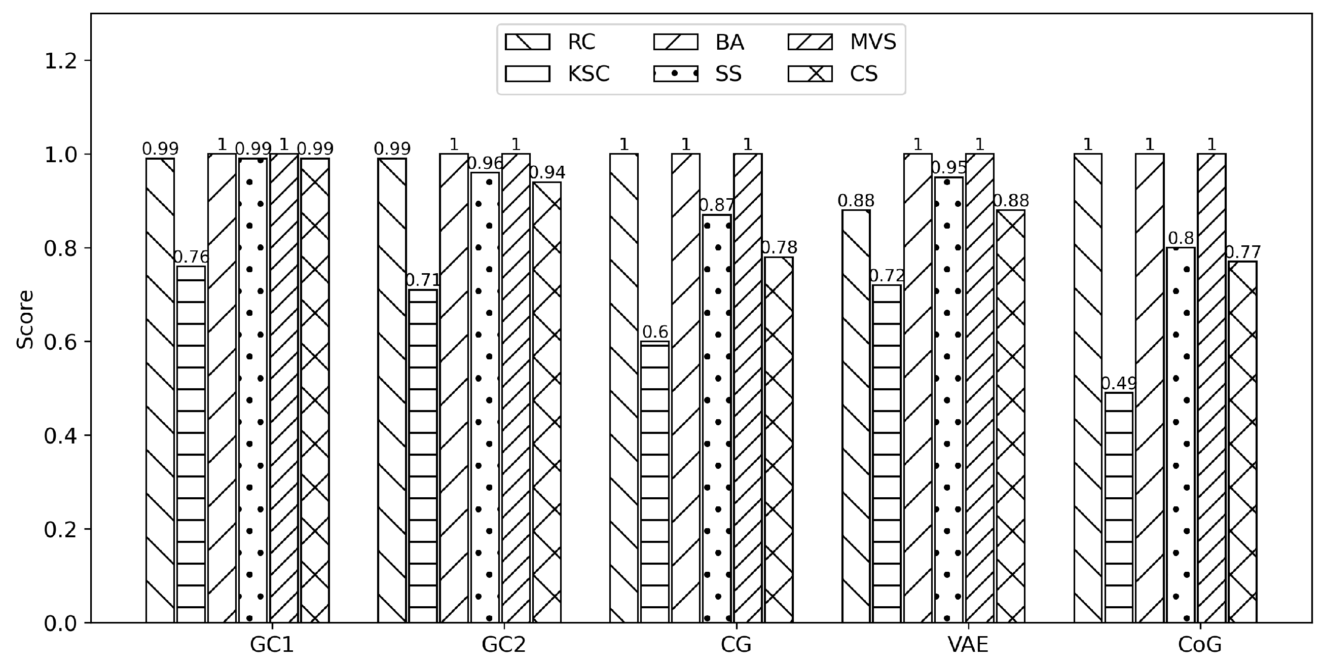
Figure 1 shows scores of the six metrics implemented to quantify the statistical and probability aspects of the five synthetic datasets.
As seen from
Figure 1 three metrics must pay attention to. The KSC metric presents a score of 0.76, 0.71, and 0.72 in GC1, GC2, and VAE for a moderate similarity between the original and the synthetic columns. In contrast, in CG and CoG the scores are 0.6 and 0.49 for divergence between the original and synthetic data. The CS metric presents a score of 0.78, 0.88, and 0.77 for CG, VAE, and CoG for a moderate correlation between original and synthetic columns. Lastly, the SS metric presents a score of 0.87 and 0.8 for CG and CoG for moderated statistical similarity (summary of observations) between the original and synthetic columns.
3.2. Feature Scaling
For each of the five sets of multivariate synthetic data, attributes divided in CBG as dependent (factor to understand or predict) and independent Spo2, pr-bpm, temp, and 24 BIA modules and phases (features that have an impact on the dependent attribute) to handled for standardization with the three feature scaling techniques min-max, standard, robust. Some literature studies hold up the effect of data scaling on the performance of machine learning algorithms [
33]. Thus,
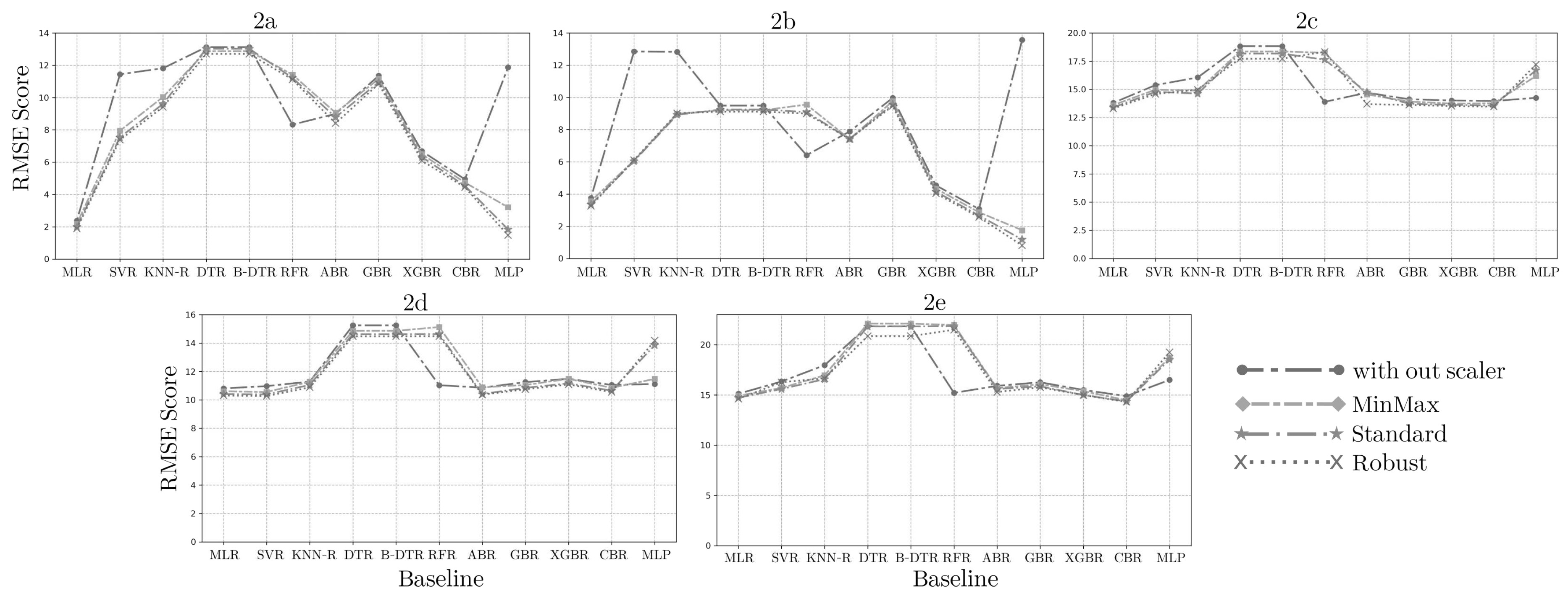
Figure 2 shows the impact of the three data scaling techniques applied in the five synthetic datasets and evaluated within the eleven machine learning algorithms of the baseline to find the best scaler matching.
As observed in
Figure 2a, the GC1 synthetic dataset fits the min-max scaler for MLR, DTR, BTR, and GB-R, the standard scaler for RFR and MLP-R, and the robust scaler for SVR, KNN, AB-R, XGB-R, and CB-R. For GC2 synthetic dataset,
Figure 2b shows that the min-max scaler fits for MLR, SVR, KNN, RFR, DTR, BTR, AB-R, GB-R, XGB-R, and CB-R, standard scaler for MLP-R. For CG synthetic dataset,
Figure 2c shows that the min-max scaler fits for MLR, GB-R, XGB-R, and CB-R, the standard scaler for KNN, RFR, and MLP-R, and the robust scaler for SVR, DTR, BTR, and AB-R. For VAE synthetic dataset,
Figure 2d shows that the min-max scaler fits for MLR, SVR, GB-R, and CB-R, the standard scaler for KNN, AB-R, XGB-R, and MLP-R, and the robust scaler for DTR, BTR, and RFR. For CoG synthetic dataset,
Figure 2e shows that the min-max scaler fits for MLR, SVR, GB-R, and CB-R, the standard scaler for KNN, XGB-R, and MLP-R, and the robust scaler for DTR, BTR, RFR, and AB-R.
3.3. Feature Selection
Finding out the appropriate scaler for each model in the synthetic datasets is essential to obtain the features set with the best performance. Sequential feature selection (SFS) is the method used to avoid over-fitting by reducing the features subset for each AI model of the baseline starting with ten features until completing forty-five, incrementing in five units. In each round, a dataset with reduced features is obtained and split into train and test sets with an 80-20% ratio. Grid, Random, and Bayes search approaches accomplish hyperparameters optimization of all baseline models. The best-optimized hyperparameters are used with the reduced features to perform training and inference on each model. Subsequently, each baseline regression model was evaluated with the reduced features as inputs, both the training and test sets. The MAE, MSE, RMSE, and
error metrics quantify the model performance in predicting glucose. Also, k-fold cross-validation, with k=5, was used to evaluate each AI model on a limited unseen data sample.
Table 2 shows the outcomes of the feature selection procedure with the best AI models performance on GC1, GC2, CG, VAE, and CoG synthetic datasets.
3.4. Selection and performance of the best synthetic datasets
After evaluation, features in common among the best models (AI Model column on
Table 2) were identified and selected on each synthetic dataset. From GC1, fifteen features are in common. From GC2, eight are similar. Thirteen are in common in CG. From VAE, twelve are in common, and from CoG, twenty-two are in common. With features in common identified, an optimum model can be found and used as a diabetes predictor. Thus, an optimum model implies evaluating all AI models of the baseline with the reduced features in common regarding MAE, MSE, RMSE,
error metrics, and k-fold cross-validation.
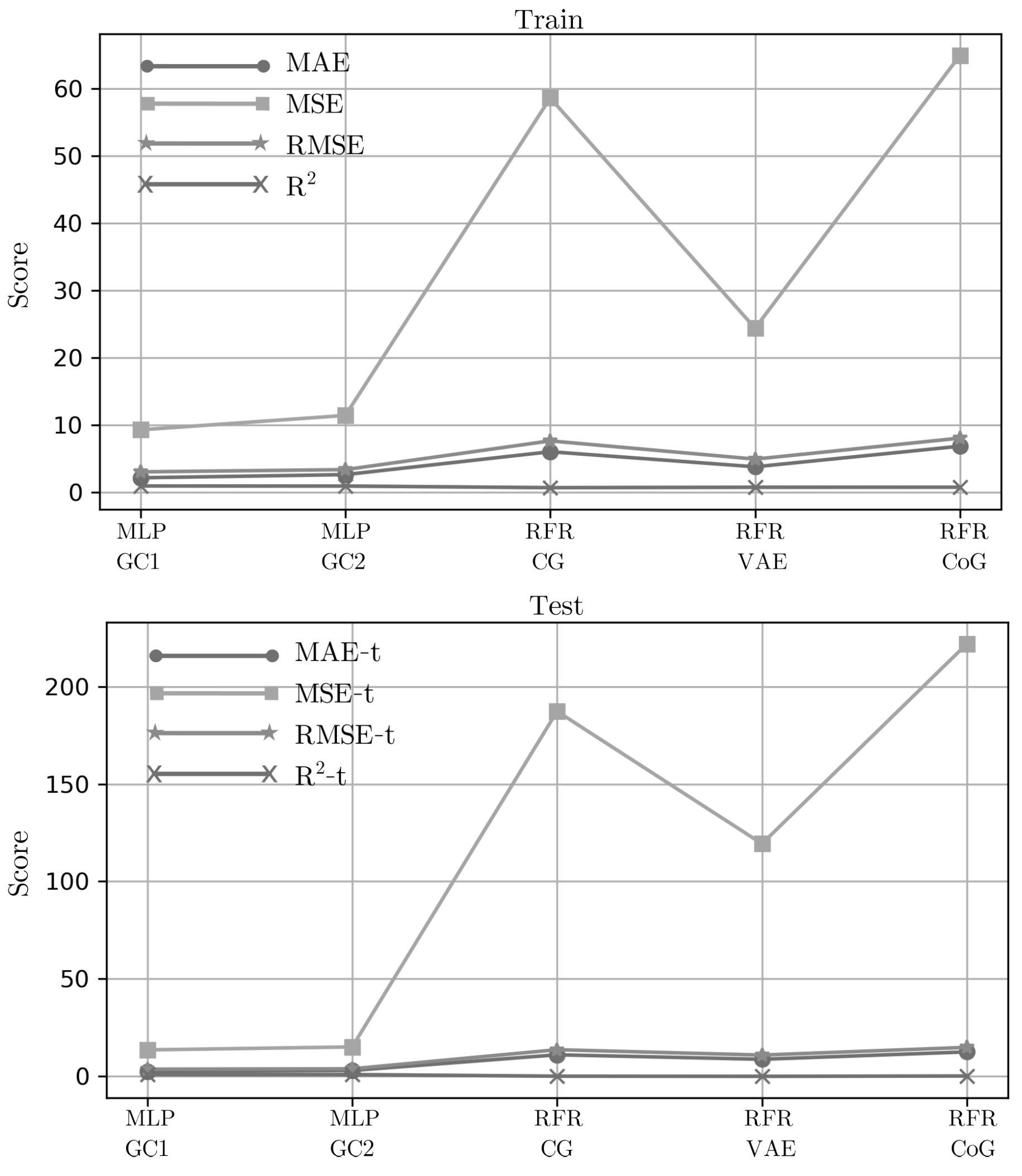
Figure 3 shows the performance of the optimum model using the reduced features in common for each synthetic dataset.
The performance of the 15-features in GC1 revealed that MLP outperformed with 2.17, 2.51 in MAE; 9.29, 13.59 in MSE; 3.05, 3.69 in RMSE, and 0.95, 0.92 in , respectively, on training and test sets. For the performance of 8-features in GC2, MLP was the best with 2.64, 3.02 in MAE; 11.43, 15.11 in MSE; 3.38, 3.89 in RMSE, and 0.94, 0.92 in respectively, on the training and test sets. Grid-search optimization method allows the hyperparameters tuning in both MLP models. The MLP in GC1 was implemented with one hidden layer (16 neurons), fully connected with a rectified linear unit activation function, quasi-newton optimizer, and L2 regularization of 0.05. The MLP in GC2 was implemented with one hidden layer (50 neurons), fully connected with a rectified linear unit activation function, quasi-newton optimizer, and L2 regularization of 0.05.
On the other hand, the performances of the 13, 12, and 22 features in common for CG, VAE, and CoG, respectively, were better with RFR in the training sets, but a poor performance on the test set, which is known as the problem of model performance mismatch. In the CG dataset, RFR shows 6.04, 11.06 in MAE; 58.58, 187.28 in MSE; 7.65, 13.68 in RMSE, and 0.70, 0.10 in on training and test sets respectively. In the VAE dataset, RFR shows 3.80, 8.76 in MAE; 24.38, 119.35 in MSE; 4.94, 10.92 in RMSE, and 0.76, 0.03 in respectively on training and test sets. Finally, in the CoG dataset, RFR shows 6.04, 11.06 in MAE; 58.58, 187.28 in MSE; 7.65, 13.68 in RMSE, and 0.70, 0.10 in respectively on training and test sets. Results indicate that synthetic data generated with methods based on GANs and autoencoders do not fit properly to perform accurate inferences.
3.5. Exploratory data analysis of the best synthetic datasets and Optimal models
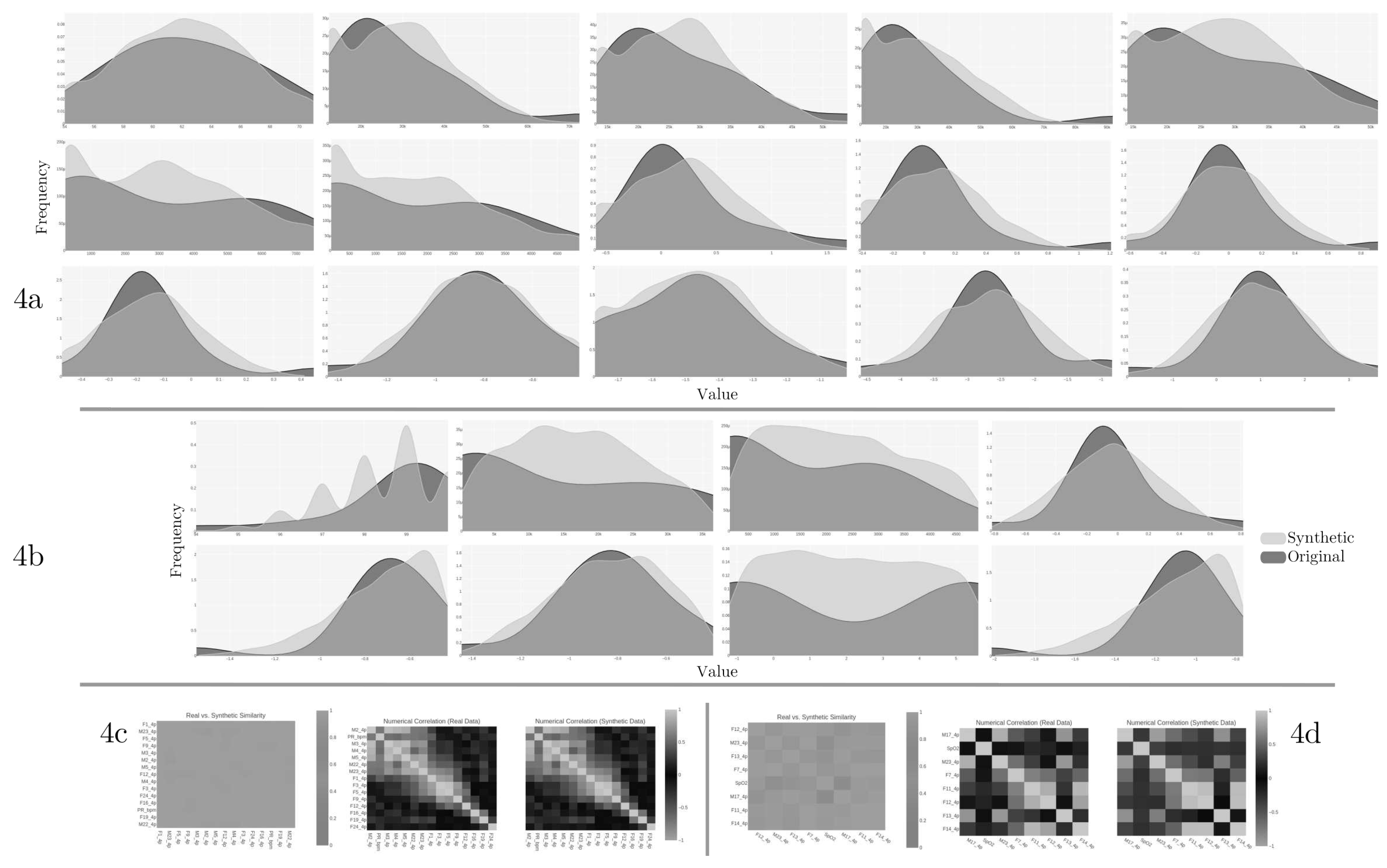
The quality report from the results of reduced features in GC1 and GC2 summarizes the similarity and correlation of original and synthetic data distributions.
Figure 4 shows the original columns against the same synthetic ones in GC1 (
4a) and GC2 (
4b). The quality report of GC1 retrieves an overall score of 0.88558 (equivalent to 88.56%), and the overall score of GC2 retrieves 0.82571 (82.57% of quality). For the case of the correlation metric,
Figure 4 shows the trend between the columns regarding Pearson and Spearman ranking coefficients in GC1 (
4c) and GC2 (
4d). The higher the score, the more the trends are alike. According to the diagnostic report description, both synthetic datasets (GC1 and GC2) cover over 90% of the numerical ranges present in the original data, over 90% of the synthetic rows are not copies of the original data, and the synthetic data follows over 90% of the min/max boundaries set by the original data.
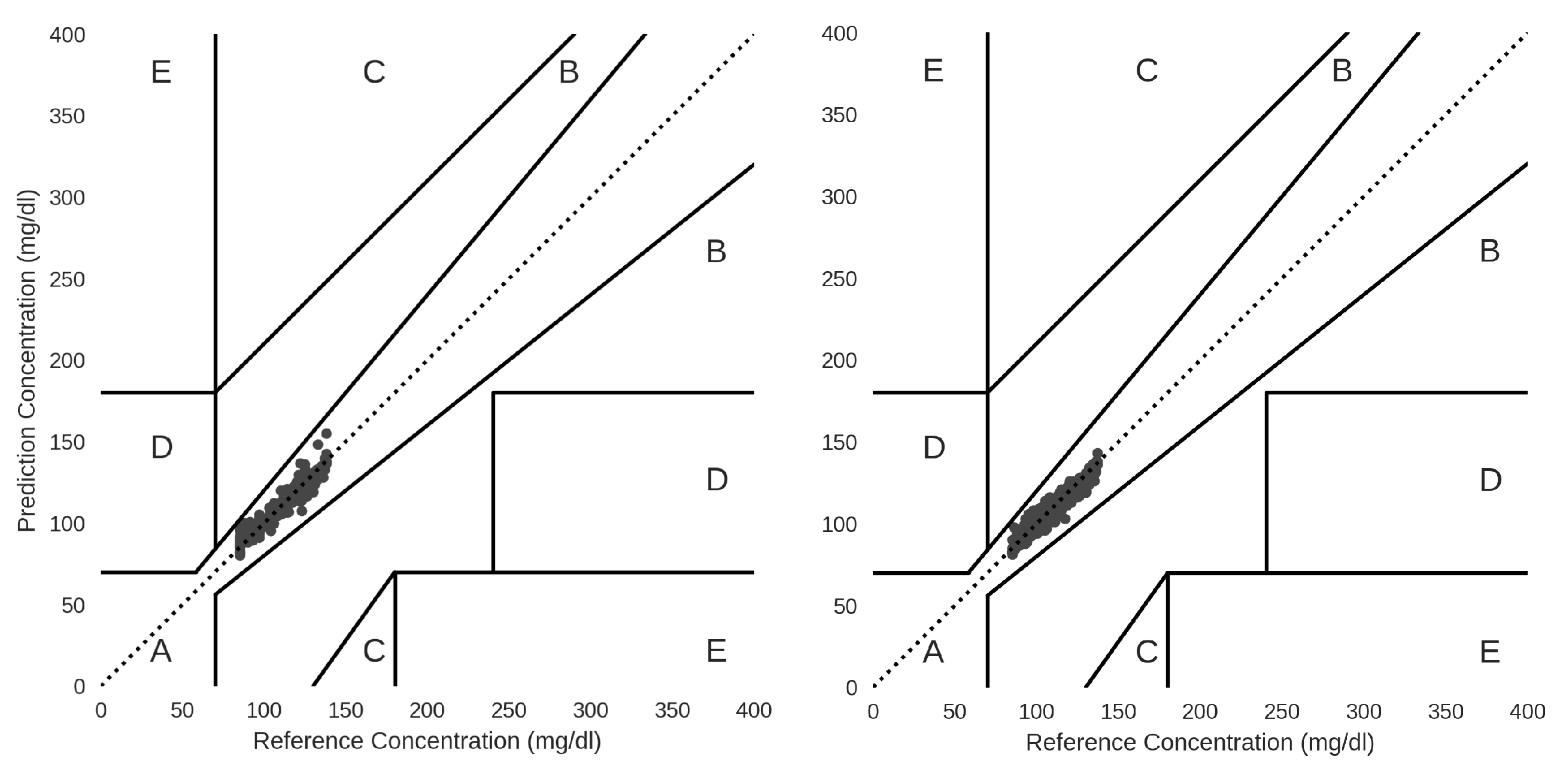
Optimal MLP models from GC1 and GC2 were used to make inferences and predict glucose. Inference results when applying Clarke Error Grid Analysis (CEGA), which is an essential tool to estimate and check the clinical accuracy of self-monitoring of blood glucose (SMBG) monitors, the predicted values for GC1 and GC2 with MLP fall in zone A, indicating that these values are within the sensor’s reference rate by +-10%.
Figure 5 shows that values within this range are considered clinically accurate.
4. Discussion
Among the possible causes of the performance mismatch issue, two options emerge: model overfitting and the quality of the data sample. To check for overfitting, different hyperparameters found by the optimization techniques were tested with the models in the train/test sets and k-fold cross-validation. For data sample quality, the synthetic datasets CG, VAE, and CoG are an unrepresentative sample of data. When plotting CG and CoG generator and discriminator loss values varying over epochs and batch size parameters of the neural network.
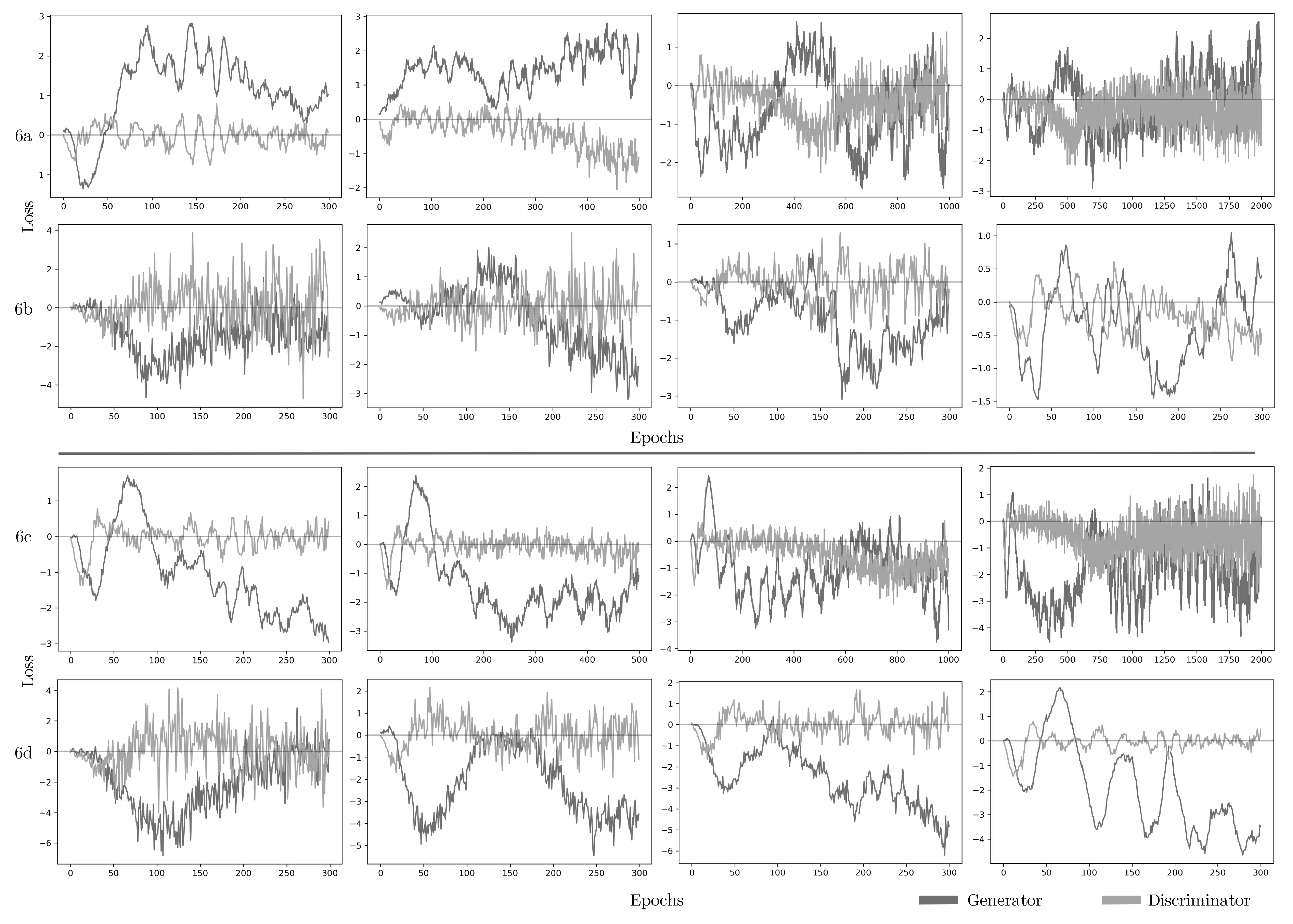
GANs improve over time, and the loss functions tell how each network improves after each training iteration or epoch. The discriminator and generator each have their loss values. Epoch-after-epoch the networks learn by trying to minimize their loss function. The discriminator learns when producing low values, around zero, if the data is synthetic and high values if it is original. The generator loss tends to be a negative value over time.
Figure 6 shows tests in epochs and batch size parameters for CG and CoG with different values.
Figures 6a and
6b shows the behavior of the discriminator and generator in CG and CoG using epochs in intervals of 300, 500, 1000, and 2000 with the batch size fixed at 500 (default value).
Figures 6c and
6d, in contrast, show the behavior of the discriminator and generator in CG and CoG using epochs fixed at 300 (default value) with batch size in intervals of 10, 50, 100, and 1000. According to the results in
Figure 6, loss values are not stabilizing, indicating that the CG and CoG methods do not learn patterns in the original data. The loss values are not only failing to stabilize, but they are getting noisier over time. Thus, the data itself might not be suitable for CG and CoG.
In the case of VAE,
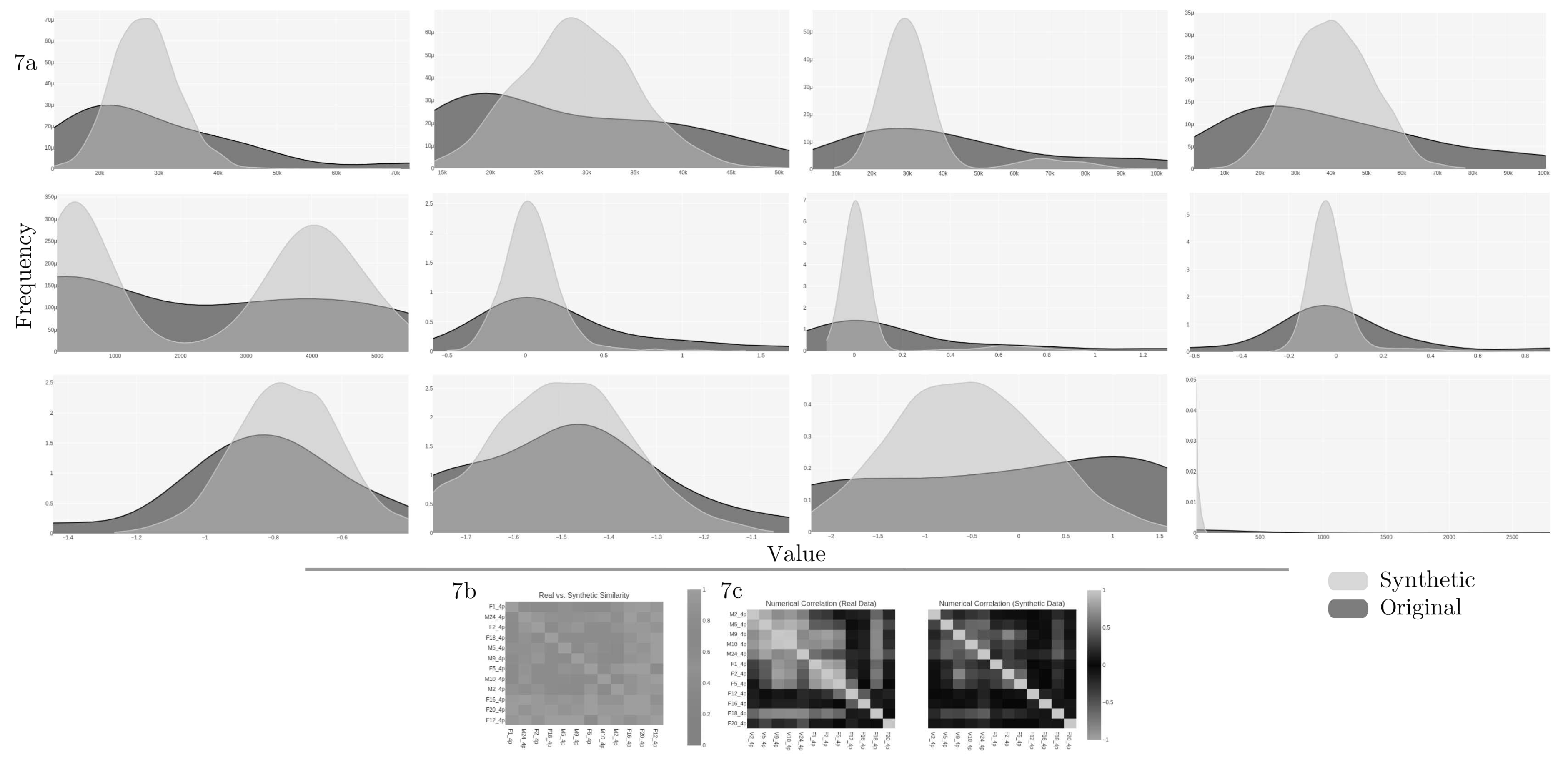
Figure 7a shows the quality report of the synthetic dataset with the original columns against the same synthetic from the twelve features in common. The quality report retrieves an overall score of 0.7756 (equivalent to 77.56%) and a column shapes score of 0.6729 (or 67.3%).
For the correlation metric,
Figures 7b shows that there is no trend between the columns regarding Pearson and Spearman ranking (
7c coefficients. The diagnostic report discloses that over 90% of the synthetic data are not copies of the original, and synthetic data follows over 90% of the min/max boundaries set by the original. However, the synthetic data is missing more than 10% of the numerical ranges present in the original data.
5. Conclusion
In this work, it was generated synthetic datasets for non-invasive diabetes prediction. Classical and machine learning-based synthetization techniques incorporate different combinations of learning rates and batch sizes for Copulas, GAN, and VAE training and generation performance. Fixed batch size to 500 and epoch intervals of 300, 500, 1000, and 2000. Fixed epochs at 300 with batch size intervals of 10, 50, 100, and 1000. Experimental results recommend the Copulas method to generate a synthetic dataset that builds normal distributions of multiple variables by analyzing the dependencies between their distributions to expand the original dataset. In addition to the optimal model, four models allow diabetes prediction within GC1 and GC2 synthetic datasets. For GC1 the models MLR, GBR, SVR, and XGBR. From GC2 was identified CB, RFR, MLR, and GBR. Analysis of the four regressors, when trained on the synthetic dataset (GC1 and GC2), shows that the availability of more training data helps improve the prediction of the regressor while achieving relatively high sensitivity. Thus, inflating the size of the training data enhances the performance of machine learning regressors. As an initial inquiry, this research limits itself to one GAN architecture and one data set. Future work needs to verify methods based on GAN and autoencoders to allow the generation of reliable synthetic data. Explore deep learning network architectures and datasets with diverse characteristics. Perform tests with additional configurations of hyperparameters that control the learning behavior and impact the model performance in generated data and computational time.
In this work, it was designed custom hardware to perform non-invasive measurements for diabetes prediction. A custom design allows the selection of every component to get the best performance. From the AI models’ baseline, the reduced features with GC1 and GC2 show lowered inputs for bioimpedance analysis. Another advantage of the customized hardware is extensive control of every aspect related to custom single-frequency and multifrequency waveform excitation signals, digital filters, and other features performed with a microcontroller.
In conclusion, by looking at the near future, envision a new era of smart health collecting real-world data evidence from wearable devices. The review showed that synthetic data has the potential to bridge data access gaps. The examples cited in this review highlighted the utility of synthesized health data in different areas of health research. The availability of publicly available synthetic health datasets and off-the-shelf synthetic data generators reflects the growing interest and demand for accessible data. Synthetics techniques describe a solution to the problem of reduced data when developing machine learning models to predict healthcare events. Results demonstrate the capability of the copulas model to expand reduced datasets preserving their intrinsic characteristics for non-invasive diabetes prediction. As found in this study, dataset augmentation provides the potential to realistically augment small and imbalanced datasets, leading to a general improvement in the predictive performance of machine learning models.
Funding
Funding for this research was provided by FAPESC under the number 2021TR2264 (Fundação de Amparo à Pesquisa e Inovação do Estado de Santa Catarina) and developed at Universidade do Estado de Santa Catarina (UDESC).
Acknowledgments
We thank the Fundação de Amparo à Pesquisa e Inovação do Estado de Santa Catarina (grant number 2021TR2264) and the State University of Santa Catarina by its institutional support.
Conflicts of Interest
The authors declare no conflict of interest.
References
- Organization-WHO, W.H. Classification of diabetes mellitus; WHO Press: Geneva, 2019. [Google Scholar]
- Federation-IDF, I.D. IDF Diabetes Atlas 10th edition; IDF Press: Belgium, 2021. [Google Scholar]
- Organization-WHO, W.H. Management of diabetes mellitus standards of care and clinical practice guidelines; WHO Press: Geneva, 1994. [Google Scholar]
- Pleus, S.; Freckmann, G.; Schauer, S.; Heinemann, L.; Ziegler, R.; Ji, L.; Mohan, V.; Calliari, L.E.; Hinzmann, R. Self-Monitoring of Blood Glucose as an Integral Part in the Management of People with Type 2 Diabetes Mellitus. Diabetes Therapy 2022. [Google Scholar] [CrossRef]
- Makroum, M.A.; Adda, M.; Bouzouane, A.; Ibrahim, H. Machine Learning and Smart Devices for Diabetes Management: Systematic Review. Sensors 2022, 22. [Google Scholar] [CrossRef]
- Nomura, A.; Noguchi, M.; Kometani, M.; Furukawa, K.; Yoneda, T. Artificial Intelligence in Current Diabetes Management and Prediction. Current Diabetes Reports 2021, 21. [Google Scholar] [CrossRef]
- Ellahham, S. Artificial Intelligence: The Future for Diabetes Care. The American Journal of Medicine 2020, 133, 895–900. [Google Scholar] [CrossRef]
- Vettoretti, M.; Cappon, G.; Facchinetti, A.; Sparacino, G. Advanced Diabetes Management Using Artificial Intelligence and Continuous Glucose Monitoring Sensors. Sensors 2020, 20. [Google Scholar] [CrossRef]
- Huang, R.; Feng, W.; Lu, S.; shan, T.; Zhang, C.; Liu, Y. An artificial intelligence diabetes management architecture based on 5G. Digital Communications and Networks 2022. [Google Scholar] [CrossRef]
- Stolfi, P.; Valentini, I.; Palumbo, M.C.; Tieri, P.; Grignolio, A.; Castiglione, F. Potential predictors of type-2 diabetes risk: machine learning, synthetic data and wearable health devices. BMC Bioinformatics 2020, 21. [Google Scholar] [CrossRef]
- Hyun, J.; Lee, Y.; Son, H.M.; Lee, S.H.; Pham, V.; Park, J.U.; Chung, T.M. Synthetic Data Generation System for AI-Based Diabetic Foot Diagnosis. SN Computer Science 2021, 2. [Google Scholar] [CrossRef]
- Dahmen, J.; Cook, D. SynSys: A Synthetic Data Generation System for Healthcare Applications. Sensors 2019, 19. [Google Scholar] [CrossRef]
- Noguer, J.; Contreras, I.; Mujahid, O.; Beneyto, A.; Vehi, J. Generation of Individualized Synthetic Data for Augmentation of the Type 1 Diabetes Data Sets Using Deep Learning Models. Sensors 2022, 22. [Google Scholar] [CrossRef]
- Hargreaves, C.A.; Heng, W.L.E. Simulation of Synthetic Diabetes Tabular Data Using Generative Adversarial Networks. Clinical Medicine Journal 2021, 7. [Google Scholar]
- Ross, S. The Multivariate Normal Distribution and Copulas. In Simulation, Fifth ed.; Ross, S., Ed.; Academic Press, 2013; pp. 97–109. [Google Scholar] [CrossRef]
- Wang, Z.; Myles, P.; Tucker, A. Generating and evaluating cross-sectional synthetic electronic healthcare data: Preserving data utility and patient privacy. Computational Intelligence 2021, 37, 819–851. [Google Scholar] [CrossRef]
- Goodfellow, I.J.; Pouget-Abadie, J.; Mirza, M.; Xu, B.; Warde-Farley, D.; Ozair, S.; Courville, A.; Bengio, Y. Generative Adversarial Nets. Proceedings of the 27th International Conference on Neural Information Processing Systems - Volume 2; MIT Press: Cambridge, MA, USA, 2014; pp. 2672–2680. [Google Scholar]
- Lan, L.; You, L.; Zhang, Z.; Fan, Z.; Zhao, W.; Zeng, N.; Chen, Y.; Zhou, X. Generative Adversarial Networks and Its Applications in Biomedical Informatics. Frontiers in Public Health 2020, 8. [Google Scholar] [CrossRef] [PubMed]
- Kingma, D.P.; Welling, M. Auto-Encoding Variational Bayes. 2022, arXiv:stat.ML/1312.6114]. [Google Scholar]
- Lee, D.; Yu, H.; Jiang, X.; Rogith, D.; Gudala, M.; Tejani, M.; Zhang, Q.; Xiong, L. Generating sequential electronic health records using dual adversarial autoencoder. Journal of the American Medical Informatics Association 2020, 27, 1411–1419. [Google Scholar] [CrossRef]
- Biswal, S.; Ghosh, S.; Duke, J.; Malin, B.; Stewart, W.; Xiao, C.; Sun, J. EVA: Generating Longitudinal Electronic Health Records Using Conditional Variational Autoencoders. In Proceedings of the 6th Machine Learning for Healthcare Conference; Jung, K., Yeung, S., Sendak, M., Sjoding, M., Ranganath, R., Eds.; PMLR. 2021; Vol. 149, Proceedings of Machine Learning Research. pp. 260–282. [Google Scholar]
- Duboue, P. The Art of Feature Engineering: Essentials for Machine Learning; Cambridge University Press, 2020. [Google Scholar] [CrossRef]
- Ahsan, M.M.; Mahmud, M.A.P.; Saha, P.K.; Gupta, K.D.; Siddique, Z. Effect of Data Scaling Methods on Machine Learning Algorithms and Model Performance. Technologies 2021, 9. [Google Scholar] [CrossRef]
- Dong, G.; Liu, H. Feature Engineering for Machine Learning and Data Analytics, 1st ed.; CRC Press, Inc.: USA, 2018. [Google Scholar]
- Ellahham, S. Artificial Intelligence: The Future for Diabetes Care. The American Journal of Medicine 2020, 133, 895–900. [Google Scholar] [CrossRef]
- Xie, J.; Wang, Q. Benchmarking Machine Learning Algorithms on Blood Glucose Prediction for Type I Diabetes in Comparison With Classical Time-Series Models. IEEE Transactions on Biomedical Engineering 2020, 67, 3101–3124. [Google Scholar] [CrossRef]
- Anand, P.K.; Shin, D.R.; Memon, M.L. Adaptive Boosting Based Personalized Glucose Monitoring System (PGMS) for Non-Invasive Blood Glucose Prediction with Improved Accuracy. Diagnostics 2020, 10. [Google Scholar] [CrossRef]
- Shokrekhodaei, M.; Cistola, D.P.; Roberts, R.C.; Quinones, S. Non-Invasive Glucose Monitoring Using Optical Sensor and Machine Learning Techniques for Diabetes Applications. IEEE Access 2021, 9, 73029–73045. [Google Scholar] [CrossRef]
- Sen Gupta, S.; Kwon, T.H.; Hossain, S.; Kim, K.D. Towards non-invasive blood glucose measurement using machine learning: An all-purpose PPG system design. Biomedical Signal Processing and Control 2021, 68, 102706. [Google Scholar] [CrossRef]
- Makroum, M.A.; Adda, M.; Bouzouane, A.; Ibrahim, H. Machine Learning and Smart Devices for Diabetes Management: Systematic Review. Sensors 2022, 22. [Google Scholar] [CrossRef] [PubMed]
- Bogue-Jimenez, B.; Huang, X.; Powell, D.; Doblas, A. Selection of Noninvasive Features in Wrist-Based Wearable Sensors to Predict Blood Glucose Concentrations Using Machine Learning Algorithms. Sensors 2022, 22. [Google Scholar] [CrossRef] [PubMed]
- Agrawal, H.; Jain, P.; Joshi, A.M. Machine learning models for non-invasive glucose measurement: towards diabetes management in smart healthcare. Health and Technology 2022, 12. [Google Scholar] [CrossRef] [PubMed]
- Ambarwari, A.; Jafar Adrian, Q.; Herdiyeni, Y. Analysis of the Effect of Data Scaling on the Performance of the Machine Learning Algorithm for Plant Identification. Jurnal RESTI (Rekayasa Sistem dan Teknologi Informasi) 2020, 4, 117–122. [Google Scholar] [CrossRef]
|
Disclaimer/Publisher’s Note: The statements, opinions and data contained in all publications are solely those of the individual author(s) and contributor(s) and not of MDPI and/or the editor(s). MDPI and/or the editor(s) disclaim responsibility for any injury to people or property resulting from any ideas, methods, instructions or products referred to in the content. |
© 2020 by the authors. Licensee MDPI, Basel, Switzerland. This article is an open access article distributed under the terms and conditions of the Creative Commons Attribution (CC BY) license (https://creativecommons.org/licenses/by/4.0/).
