Detecting Human Gait Metabolism Disorders Based on A Novel Criticality Analysis Methodology

Preprint

Article

Detecting Human Gait Metabolism Disorders Based on A Novel Criticality Analysis Methodology

Altmetrics

Downloads

128

Views

Comments

A peer-reviewed article of this preprint also exists.

Supplementary Material

supplementary.zip (2.36MB )

Submitted:

22 August 2023

Posted:

24 August 2023

You are already at the latest version

Alerts

Abstract

The way in which a person walks, known as human gait, is a significant indicator of overall health and well-being. Abnormalities in gait can indicate the presence of metabolic disorders, such as diabetes or obesity. However, detecting these disorders can be challenging using traditional methods, which often involve subjective assessments or invasive procedures. In this study, a novel methodology known as Criticality Analysis (CA) was proposed for the detection and monitoring of human gait in people with metabolic disorders taking part in an intervention to increase activity and reduce weight. The CA approach utilised inertial measurement unit gait data, alongside clinical health measures. This allows for the control of nonlinear growth in the system, resulting in lower dimensional, nonlinear, free-scale, stable, controlled, and organised trajectories. These trajectories were then analysed using a Support Vector Machine (SVM) algorithm, which is well-suited for this task due to its ability to handle nonlinear and dynamic data. The combination of the CA approach and the SVM algorithm demonstrated high accuracy and non-invasiveness in detecting metabolic disorders, yielding an average accuracy within the range of 78.2% to 90%. Additionally, the classification technique accuracy, at a group level was observed to reduce during period of the intervention (e.g., from week 2 to week 3) alongside changes in fitness and health, which indicates the potential of using the approach to measure and monitor biological systems. As such, this novel methodology has the potential to be a valuable tool for healthcare professionals in detecting and monitoring metabolic disorders, as well as other unknown diseases associated with the human biological system.

Keywords:

Subject: Computer Science and Mathematics - Artificial Intelligence and Machine Learning

1. Introduction

Gait, which is also referred to as human locomotion, is the manner in which an individual moves their body while walking or running [1]. It is a crucial aspect of human movement and can provide valuable insights into the overall health and well-being of an individual. From a medical perspective, gait analysis is used to evaluate and diagnose disorders or diseases that affect the musculoskeletal and neurological systems [2]. These disorders can include conditions such as arthritis, Parkinson’s disease, and cerebral palsy, among others. However, the complexity of the human gait, as well as the numerous variables that can affect it, can make it a challenging task for medical professionals to diagnose gait disorders accurately and efficiently [3]. The variability that exists between individuals, due to factors such as age, sex, and body composition, can affect the way a person walks, making it difficult to establish a standard for normal gait. Furthermore, the intricate interplay between different body systems, including the musculoskeletal, neurological, metabolic and cardiovascular systems, can make it challenging to pinpoint the exact cause of a gait disorder [4].

Artificial intelligence (AI) and machine learning (ML) methods have the potential to revolutionise the field of gait analysis by providing a more accurate and efficient means of detecting and diagnosing gait disorders. These technologies can analyse large amounts of data, identify patterns and correlations that may not be immediately apparent to human analysts, and make predictions based on this information. The ability of AI and ML methods to process and analyse data quickly and accurately can aid medical professionals in identifying gait disorders in their early stages, leading to more effective treatment and better outcomes for patients [5].

The human body is a complex biosystem that is affected by a wide variety of internal and external factors [6]. When something happens to disturb this biosystem, the human gait can be affected, leading to a range of disorders and diseases. The need for automated tools to diagnose these disorders is imperative for early detection and prevention of different disorders reflected in gait. The ability of the criticality analysis system to quickly and accurately detect gait disorders can aid medical professionals in providing early and effective treatment, leading to better outcomes for patients. Furthermore, it can empower individuals to take charge of their own health, by providing them with the ability to manage their health conditions [7].

The novel proposed criticality analysis (CA) system in this paper is a robust technique that can assist medical professionals in the diagnosis of gait disorders. This system is based on the principle of criticality, which refers to the state of a system that is close to a critical point of instability. By analysing the gait patterns of a patient and identifying any deviations from the norm, the criticality analysis system can indicate the presence of a disorder or disease. The system can also be used to monitor the progression of a disorder and track the effectiveness of treatment over time.

The CA system is built upon the Rate Control of Chaos (RCC) principle, allowing for the maintenance of dynamic regulation of complex nonlinear behaviours in biological systems even amidst chaotic disruption [8]. This is achieved through the stabilising capability of the RCC mechanism in the face of chaos. Through mathematical modelling using a set of variables to depict the operation of variable quantities and deduce system properties, the RCC approach incorporates a set of rate equations for the system variables to not only depict how the system variable quantities change over time based on their initial state, but also to control the chaotic behaviour of the system. The control term, which can be at least one of the rate equation variables, is dominated by nonlinear variable components that greatly impact the stability of the overall global system and thus enable the system to expand exponentially [9]. The rate control function, derived from the proportions of the contributing variables to the growth rate of the rate equation, is then applied to the control term to maintain a stable control component for the rate of change equation by limiting the control term with respect to the divergence rate of the given variable. The rate control function determines the intensity of control applied to the entire system. The output of nonlinear relationships in the rate equations, which create nonlinear representation spaces from observations affecting the biological system, are utilised as input features for various machine learning techniques, such as Support Vector Machine, as demonstrated in this paper.

The paper is structured as follows: Section 2 provides an overview of human gait criticality analysis. Section 3 presents the mathematical model for criticality analysis in human walking. Section 4 reviews current SVM-based methods in human gait analysis with a focus on criticality analysis. Section 5 outlines the technical aspects of the SVM algorithm. In Section 6, the methodology of the CARDIGAN dataset is discussed, including data collection, feature extraction, criticality analysis data representation, spatiotemporal analysis, and SVM model implementation in a longitudinal study. The confusion matrix is used as a performance measure. Section 7 examines the experimental results of the CARDIGAN dataset, including the Receiver Operating Characteristic (ROC) Curve, the Area Under the Curve (AUC), and the decision boundary of the support vector method. Section 8 summarises the overall results. Finally, Section 9 concludes the main findings of the research.

2. Criticality Analysis in Human Gait

For many years, researchers have been engaged in the pursuit of understanding the intricacies of biological systems, which represent self-organised, dynamic states of living matter. These states include spatial, temporal, and spatiotemporal structures that can be found in both living and non-living materials. The presence of nonlinear phenomena, such as patterns, oscillatory modes, and traveling and spiralling waves in biological systems is widespread, and these phenomena evolve in space and time [10].

Mathematically, understanding the dynamic properties of biological functions is essential. While some states of biological systems maintain stability, they tend to display a high level of chaotic behaviour when they deviate from equilibrium due to nonlinear interactions between biological functions [11]. To fully grasp the complex functions of such systems, the development of theoretical mathematical models is imperative in order to accurately depict the nonlinear effects of biological interactions and comprehend the motions of small atoms and the concentration of biochemical reactions in biological cells.

The primary objective of this paper is to quantitatively analyse the spatiotemporal patterns of human gait when the biological system is activated by internal or external perturbations. The human motor system, a subset of the global biosystem, is physiologically complex, and there currently exists no mathematical model that can accurately characterise its dynamics in both temporal and spatial dimensions. Disruption of normal gait leads to the entire dynamic state of the biosystem drifting chaotically to a more critical state as a result of an excessive rise in kinetic energy, and the behaviour may display near power-law and exponential interactions.

To control fluctuations in the dynamics of the biosystem, the RCC method has been proven to be a robust technique for stabilising dynamic systems by controlling the dynamics of chaotic systems [12]. A chaotic system is a type of system that exhibits sensitive dependence on initial conditions, meaning that small differences in initial conditions can lead to vastly different outcomes over time. This makes chaotic systems difficult to predict and control [11]. The RCC method is based on the idea of controlling the rate of change of a chaotic system by adjusting certain parameters of the system. This can be done by using techniques such as feedback control or coupling [13]. By controlling the rate of change of the system, it is possible to stabilise the chaotic dynamics and bring the system to a desired state or behavior. The RCC method has been applied in various fields such as physics, chemistry, and engineering, but it is rarely applied in human gait analysis or bio-mechanics.

This innovative approach provides a promising solution for comprehending the behaviour of dynamic systems affecting gait by creating controlled and stabilised representative trajectories of complex gait patterns in a lower-dimensional space, thereby unlocking the complexity of a wide range of machine learning techniques utilised for reducing the dimensionality of data.

3. Mathematical Model for Criticality Analysis in Human Gait

In order to comprehend the function of biological systems through the lens of mathematical models, it is necessary to utilise models that accurately capture the complexity of the system. Unfortunately, simplified or reduced models represented by a set of ordinary differential equations in the time domain are often inadequate in fully capturing the intricacies of the control mechanism responsible for translating network behavior into spatial outcomes in a biological system, and maintaining global stable and controlled states [11].

In this paper, the nonlinear biochemical enzyme control model is being extended for the analysis of human gait, as it draws inspiration from the traditional biochemical enzyme control concept presented in [14]. It has proven to be an effective approach for adjusting the reaction control and regulating the disturbances caused to the biosystem, which could affect other biological functions. Additionally, the nonlinear biochemical enzyme control model is a novel approach that has the potential to control the dynamic behaviour of human gait, which is a complex and physiologically intricate process. By extending the application of this model, it could offer deeper insights into the mechanisms that govern human gait, and prove beneficial in diagnosing and treating gait disorders.

The present model utilises a control mechanism to stabilise external perturbations to the motor system by precisely calibrating the quantity of enzyme in relation to the concentration of one of the variables, f. The model also represents the control process of two enzymes that govern the formation of the extracellular matrix, m, from soluble filaments, f. The proteinase, p, deconstructs the matrix into filaments, while transglutaminase, g, reassembles the filaments into the matrix. The extracellular matrix, m, is continually generated by adjacent cells,

r_{i m}

, at a constant rate, with each protein undergoing catalytic processes proportional to p. The bifurcation parameter,

r_{i m}

, acts as an external turbulent input to the control model. The rate of change of the production of enzymes p and g is determined by the RCC, which is characterised by the presence of soluble filaments, represented by f, as specified in equation 1. This is further detailed in equations 2 and 3. The output of the model is presented as a phase space manifold, with the primary varying parameter f represented on the x-axis and m represented on the y-axis. This representation demonstrates the time-dependent changes of the parameters and serves as an illustration of the nonlinear dynamics of free-scale gait patterns extracted by the model. These dynamics are subsequently utilised as input features for the support vector machine models.

q_{f} = \frac{f}{f + μ_{f}}

(1)

σ_{p} (q_{f}) = f_{p} e^{(x_{p} q_{f})}

(2)

σ_{g} (q_{f}) = f_{g} e^{(x_{g} q_{f})}

(3)

\frac{d m}{d t} = k_{g} \frac{f g}{K_{G} + f} - \frac{m p}{1 + m} + r_{i m}

(4)

\frac{d f}{d t} = - k_{g} \frac{f g}{K_{G} + f} + \frac{m p}{1 + m} - \frac{f p}{1 + f}

(5)

\frac{d p}{d t} = σ_{p} (q_{f}) γ \frac{f^{n}}{K_{R}^{n} + f^{n}} - k_{a} p^{2}

(6)

\frac{d g}{d t} = σ_{g} (q_{f}) β \frac{f^{l}}{K_{S}^{l} + f^{l}} - k_{d e g} \frac{g p}{K_{d e g} + g}

(7)

The extended CA model has several parameters, including

γ = 0.026

β = 0.00075

K_{R} = 4.5

K_{S} = 1

K_{G} = 0.1

K_{d e g} = 1.1

k_{g} = k_{d e g} = 0.05

, and

k_{a} = \frac{k_{d e g}}{K_{d e g}} = 0.0455

. The Hill-numbers n and l are also set to 4. The bifurcation parameter

r_{i m}

exhibits a wide range of dynamic behaviors, including stable periodic cycles, bistability, and chaos. This parameter remains constant for all oscillators within the chaotic domain. Additionally, an external input is applied as a perturbation to the

r_{i m}

parameter as described in Equation 8. This parameter links different oscillators together by using a relative scale contribution from all other oscillators. The RCC control parameters presented in Equations 1, 2, and 3 (

f_{p} = f_{g} = 1

x_{p} = x_{g} = - 1

, and

μ_{f} = 2

) are kept constant throughout the experiment simulations in this paper, but can have different values that allow the local oscillator to change its oscillatory orbits.

{r_{i m}}^{i} = \sum_{j = 1, j \neq i}^{n} w_{j} m_{j} + ε

(8)

The connectivity strength between various oscillators, represented by

w_{j}

, can range from

0.00011

0.00012

, to

0.00025

. External perturbations, represented by

ε

, are uniformly distributed according to a Gaussian distribution and scaled within the domain of

[- 1, 1]

. These perturbations are observed over a range of evolution steps to explore the varying oscillatory cycles they produce. In this paper, a connectivity strength of

w_{j} = 0.0002

was selected from the chaotic domain of the underlying oscillators to assess its effect on the dynamics while maintaining overall stability.

The network of nonlinear models in this paper consists of 16 oscillators, each of which can adjust their local dynamics to adapt to external perturbations from their neighboring oscillators. The simulation of the entire model was carried out using EuNeurone software and the Fehlberg-RK method as a fixed step integration for Ordinary Differential Equations (ODEs) [15]. The total unweighted dynamics, represented by M and F in equations 9 and 10, were measured as the net sum of the individual oscillators, allowing for observation by a remote observer who would otherwise be unable to detect the individual oscillators.

M = \sum_{i = 1}^{n} m_{i}

(9)

F = \sum_{i = 1}^{n} f_{i}

(10)

The proposed CA based on the RCC control technique, as presented in this model, has been demonstrated to effectively stabilise nonlinear, spatiotemporal patterns in human gait. Through rigorous examination, it has been established that this method performs exceptionally well in stabilising chaotic systems, effectively confining their behavior to stable periodic cycles, as determined by the local dynamics of each oscillator. Furthermore, the examination of human gait using this model has uncovered unique orbits, arising from perturbations in the underlying critical system composed of nonlinear controlled oscillators. The scale-free nature of these orbits allows for quantification of the non-scale-free interactions between patterns stemming from the intricate biological function of gait. Through the conduct of this analysis, structured characteristics and dynamic properties of human gait can be revealed, providing valuable insights into the underlying mechanisms of this complex biological process.

4. Related Work

4.1. A Review of Support Vector Machine-based Approaches in Human Gait Analysis with a Focus on Criticality Analysis

The field of human gait analysis has seen significant advancements in recent years, yet the application of criticality analysis and rate control of chaos remains an under-explored area of research, particularly in human gait analysis. However, the utilisation of Support Vector Machines (SVMs) as a tool for gait analysis has been well-established in the literature. Although, most of the Machine Learning (ML) methods and techniques applied to human gait analysis have focused on utilizing gait features or patterns without fully understanding their biological significance. These studies often employ ML approaches to gait data without considering the underlying complexities of human gait. But the use of criticality analysis presents an opportunity to unlock the understanding of these complexities by creating spatiotemporal patterns of gait patterns in a more interpretable space. This approach allows for a deeper understanding of the dynamics of human gait. In this section, we aim to review the existing literature on the use of SVMs in gait analysis, and its potential applications in understanding the dynamics of human gait, particularly in the light of criticality analysis. The objective of this review is to provide a thorough examination of the state-of-the-art in this field and to serve as a foundation for future research endeavors.

One of the studies, which is conducted by Wonjin et al. (2021) [16] on gait analysis for detection of initial characteristics of gait disorders is a valuable contribution to the field of gait analysis and neurological disorder diagnosis. The use of the SVM method to classify abnormal gait from a walking person, as well as the integration of gait features extracted from the individual’s walking movement using the Kinect depth camera, are both strong points of the study. The 96.52% classification accuracy achieved in the study is also noteworthy and suggests that the proposed method has a high level of performance. However, it is important to note that this study has several limitations. The sample size of the study is relatively small, which can limit the generalisability of the results to a larger population. Additionally, the study only uses one type of depth camera and it would be beneficial to test their proposed method using other types of sensors to ensure the robustness of their proposed method. Furthermore, the study does not provide any information on the cost and practicality of their proposed method. The use of a depth camera and the required computational resources may make their proposed method impractical for use in a clinical setting. It would be useful to include an analysis of the cost-effectiveness of the proposed method in future studies.

Another study conducted by Iris et al. (2010) [17] presented to detect and characterise gait abnormalities in individuals with Parkinson’s disease (PD) using wireless inertial sensor system measurements. The study utilises the physical features of pitch, roll, and yaw rotations of the foot during walking and applies the Principal Component Analysis (PCA) to select features and the SVM method to create a classification model. The study found that the model performed with over 93% sensitivity and specificity and 97.7% precision in the binary classification task of detecting the presence of PD. This suggests that the wireless inertial sensor system was able to successfully detect the presence of PD based on physical features of gait and identify the specific features that characterise parkinsonian gait. Furthermore, the use of a cost-sensitive learner in the study reflected the different costs associated with misclassifying PD and control subjects, which led to 100% specificity and precision while maintaining sensitivity of close to 89%. The study also performed a multi-class classification task of characterising parkinsonian gait by distinguishing among PD with significant gait disturbance, PD with no significant gait disturbance, and control subjects. This resulted in 91.7% class recall for control subjects and 84.6% precision for PD subjects with significant gait disturbance.

Furthermore, Nukala et al. (2015) [18] and Shibuya et al. (2015) [19] used wireless gait analysis sensors (WGAS) to perform automatic fall detection and have similar sensor designs, including a tri-axial accelerometer, 2 gyroscopes, and a micro-controller. Both studies also used two supervised machine learning techniques such as Back Propagation Artificial Neural Network (BP-ANN) and SVM for fall classification. However, there were some differences in the methodology used in these studies. Nukala et al. (2015) [18] used a total of 322 tests on young volunteers and achieved an overall accuracy of 98.2% and 98.7% with BP-ANN. On the other hand, Shibuya et al. (2015) [19] utilised SVM classifier to detect falls in real-time and achieved high fall classification accuracy (98.8% and 98.7% for different sensor positions) and high overall specificity (99.5%) and sensitivity (97.0%). However, the study conducted by Nukala et al. (2015) [18] did not provide information about the specific parameters used for the algorithm, which would have been useful to understand the results and compare them to other studies. Additionally, the study only reported the accuracy of the algorithm, without providing information about other performance metrics such as precision, recall, or F1-score. On the other hand, the study by Shibuya et al. (2015) [19] reported high fall classification accuracy (98.8% and 98.7% for different sensor positions) and high overall specificity (99.5%) and sensitivity (97.0%). The study also provided information about the specific parameters used for the algorithm, which is useful to understand the results and compare them to other studies. Additionally, the study examined the performance of the algorithm in real-time, which is important in practical applications.

In a similar vein, Huang et al. (2018) [20] presented a novel approach to gait analysis by using audio data instead of visual data. This is a significant advancement in the field as it addresses the limitations of traditional gait analysis methods, which rely on visual data and are affected by changes in clothing, visibility, and angles. The use of audio data in gait analysis is an innovative approach as it is not affected by the same limitations as visual data. The technique is based on the time differences between steps rather than frequency-based features, which are affected by changes in footwear and floor surfaces. This allows for a more robust and accurate analysis of gait. The authors used SVM technique for classification. The results showed high classification rates and excellent discriminative abilities, indicating that the method is effective in identifying individuals based on their gait.

Additionally, Hayashi et al. (2015) [21] study introduced to improve the diagnostic accuracy of lumbar spinal canal stenosis (LSS) by using gait analysis as a classification method. The study group consisted of 13 healthy individuals, 11 patients with L4 radiculopathy, and 22 patients with L5 radiculopathy. The authors used video recordings and a development program to analyse gait characteristics, and an SVM to classify L4 and L5 radiculopathy. The study found that knee extension at initial contact was slightly greater in the L4 group and a one-peak waveform pattern with the disappearance of the second peak was present in 45.5% of the L5 group. The total classification accuracy was 80.4% using the SVM, with the highest accuracy in the control group and the lowest in the L4 group. The authors concluded that their walking motion analysis system was able to identify useful factors for differentiating between healthy individuals and patients with L4 and L5 radiculopathy with a high accuracy rate. The study has several strengths, such as the use of a well-established method for gait analysis and the use of a development program to analyse gait characteristics. Additionally, the use of an SVM to classify L4 and L5 radiculopathy is a valid method and the results of the study demonstrated that this method can be useful in identifying patients with LSS. However, the study also has some limitations. Firstly, the sample size is small, which may limit the generalisability of the findings. Secondly, the study only analysed patients with L4 and L5 radiculopathy, and it is unclear if the findings would be generalisable to other types of radiculopathy or other types of spinal stenosis. Additionally, the study only used healthy individuals as the control group and it would be beneficial to also include patients with other conditions to compare the gait characteristics.

Similarly, Yoo et al. (2005) [22] proposed an automated system for classifying gender by analysing human gait patterns. Their study provided valuable insights into the application of gait analysis for gender identification. The three-stage system proposed in the study is well-structured, with the detection and extraction of the moving human body and its contour from image sequences, extraction of human gait signature using joint angles and body points, and motion analysis and feature extraction for classifying gender, providing a clear and logical progression in the analysis. The use of 2D stick figures to represent the gait signature was found to be an effective approach, as it allows for the clear visualisation of the gait patterns and allows for easy comparison between subjects. Additionally, the use of an SVM classifier to classify gender is a well-established method in machine learning, and its application in this study demonstrates the robustness and reliability of the system. The experiments performed on a large database showed a high performance of 96% for classifying gender for 100 subjects, indicating that the system is highly accurate in identifying gender based on gait patterns. This is an important finding, as it has potential applications in areas such as security and surveillance, where automated gender identification is needed. However, the study has some limitations, such as the lack of diversity in the sample population, which could limit the generalisability of the findings. Additionally, the study did not address the potential ethical implications of using gait analysis for gender identification, such as privacy concerns and potential biases in the system.

Besides, the research work presented by Begg et al. (2003) [23] is a valuable contribution to the field of gait analysis and falls prevention in the older population. The use of artificial intelligence techniques, specifically Neural Networks (NN) and SVM classifiers, for automatic identification of young and old gait types is a novel approach that has the potential to aid in early identification of at-risk gait for falls prevention. The study design is well-executed, with 12 young and 12 elderly participants being recorded and analysed using a motion analysis system and a force platform. The extraction of 24 gait parameters for training and testing the NN and SVM systems is a thorough approach that allows for a robust analysis of the data. The results of the study indicated that the SVM system has a better performance than NN with 91.7% and 83.3% respectively in distinguishing between young and elderly gait patterns. This suggested that the SVM is a more effective tool for identifying at-risk gait patterns in the older population. Additionally, the classification ability of SVM was found to be unaffected by the choice of kernel functions, further highlighting the potential of SVM for applications in gait identification for falls-risk minimisation in the elderly. However, the study is limited by the small sample size of participants, which may not be representative of the older population as a whole. Additionally, the study only included participants of a specific age range, and further research is needed to evaluate the applicability of their results to older adults outside of this range.

Likewise, the work of Si et al. (2019) [24] on the development of a wearable sensing system for studying gait dynamics is a valuable contribution to the field of bio-mechanics and human movement analysis. The proposed system, consisting of sensing shoes worn by a tester, effectively captures data on various types of movements, including standing, jumping, and walking. The use of five features extracted from foot pressure signals for motion analysis is a novel approach, and the application of SVM and fractal analysis for gait recognition is well thought-out. The testing results of the system, with an overall accuracy of 93.57% using radial basis function kernel function, were impressive and demonstrate the strong potential for gait identification using this method. The limitations of the study include the small sample size, lack of diversity in the population tested, which limits the generalisability of the results, and the lack of discussion on potential applications and how the system can be used to improve human movement understanding.

Moreover, Kamruzzaman et al. (2006) [25] presented an interesting and valuable study on the use of SVM to classify children with cerebral palsy (CP) using gait parameters. The study makes use of two gait parameters, stride length and cadence, which are known to be affected in children with CP. The results of the study showed that the SVM classifier has an overall accuracy of 96.8% when normalised by leg length and age. This is a high accuracy rate and suggests that the SVM is a useful tool for identifying CP in children. One of the strengths of the study is that it compares the performance of different classifiers, including polynomial and radial basis kernel. The study found that these two classifiers performed comparably and outperformed the others. This suggests that the choice of kernel is not a significant factor in the performance of the SVM. This is an important finding as it can inform the selection of kernel in future studies. However, there are also some limitations to their study. Firstly, the sample size of the study is relatively small, with only 30 children with CP and 30 healthy children. This limits the generalisability of the results. Secondly, the study only used two gait parameters, stride length and cadence, which may not be sufficient to fully classify children with CP.

In addition, Horst et al. (2016) [26] conducted an examination to understand the nature of intrinsic inter-session variability in gait patterns. The use of 8 healthy subjects who performed 15 gait trials at a self-selected speed on 8 different days within 2 weeks allows for a thorough analysis of the separable characteristics of gait patterns between and within individuals in repeated measurement sessions. The use of ground reaction forces and lower body kinematics as a means of quantifying each trial is a sound choice, as it allows for a detailed examination of the movement patterns of the subjects. The results of the study are analysed using an SVM classifier and the coefficient of multiple correlation approach, which are both appropriate methods for the type of data being analysed. The results showed that there are a remarkable amount of individual characteristics in human gait and that gait patterns can be assumed not to be constant over time, but rather exhibit discernible daily changes within previously stated good repeatability. This is an important finding, as it suggests that gait patterns are not always stable and may change depending on various factors such as physical or emotional state. The use of SVM results in an error-free assignment of gait patterns to the corresponding individual, which demonstrates the robustness of the method. Additionally, the classification rates of 97.3% and 59.5% for the eight-day classification of lower body joint angles and ground reaction forces, respectively, highlights the ability of the method to distinguish day-specific characteristics within the range of individual gait patterns. The potential implications of this study are that it may provide a basis for more individual and situational diagnoses or therapy for gait patterns. This could lead to more effective treatments for patients with gait disorders, as well as the ability to monitor changes in gait patterns over time.

This research paper introduces a novel paradigm by successfully applying the Support Vector Machine (SVM) algorithm in conjunction with the CA method based on the RCC approach. With a specific focus on the classification of gait data collected during a 6-minute walk, the study aims to establish the technical feasibility and credibility of this innovative approach. By meticulously optimising hyperparameters

σ

and C, SVM adeptly traverses the decision boundary landscape, augmenting its classification performance with exceptional accuracy and unwavering reliability. Notably, this research introduces unexplored avenues for gait data analysis, thereby fostering unprecedented prospects across diverse domains, including healthcare, rehabilitation, and biometric identification.

5. Fundamentals of SVM Theory

The Support Vector Machine (SVM) represents a powerful and versatile tool in the realm of machine learning. Its ability to handle non-linearly separable data and perform both binary classification and regression estimation tasks has made it a widely adopted technique in various fields such as disease diagnosis, image classification, and facial recognition [27,28,29]. The utilisation of a kernel technique in the SVM algorithm allows for the formation of a non-linear class decision boundary, which is crucial in tackling complex classification problems. The primary objective of an SVM classifier is the identification of an optimal separating hyperplane (OSH) that maximises the margin between the different classes. The kernel technique transforms the input data into a high-dimensional space, and subsequently, an OSH is created to classify the various data labels in the transformed feature space. As a result, the linear OSH leads to the formulation of a non-linear boundary in the original data input space. The data vectors closest to the OSH in the transformed space are referred to as support vectors, as they contain vital information regarding the OSH. The choice of kernel function is crucial in SVM as it greatly affects the classification accuracy. Using the right kernel can enhance the SVM’s performance, so it is important to carefully consider the nature of the data and the task at hand when selecting a kernel.

Given a training dataset,

Ω = \{(x_{i}, y_{i})\} {i = 1}^{N}

, independently drawn from a probability distribution on

(X, Y)

, where

X \in R^{m}

represents the input features and

Y \in \{- 1, + 1\}

represents the classification output, the Support Vector Machine (SVM) model can achieve optimal separation of linearly separable patterns in m-dimensional space by generating a decision function,

w^{T} ϕ (x i) + b = 0

, through the minimisation of an appropriate trade-off between the structural empirical risk and the model complexity of its optimisation problems. The optimal adjustable weight vector,

w_{\circ}

, and the optimal bias,

b_{\circ}

, of the decision function are defined when the feature vectors

x_{i}

are maximised. For any two arbitrary classes,

\{- 1, + 1\}

, the SVM finds two parallel hyperplanes that correctly classify all training data points and either maximises the distance,

\frac{2}{∥ w ∥}

, or minimises the margin,

\frac{1}{2} {∥ w ∥}^{2}

, between them. For each linearly separable case, the SVM standard classification optimisation problem can be mathematically expressed as:

\begin{matrix} min_{w, b} & \frac{1}{2} {∥ w ∥}^{2} \\ subject to & y_{i} (w^{T} ϕ (x_{i}) + b) \geq 1 \end{matrix}

(11)

The SVM classifier, represented by the equation

y_{i} = sign (w^{T} ϕ (x_{i}) + b)

, is utilised to assign each class to either side of the hyperplane. The minimum value of

(w^{T} ϕ (x_{i}) + b)

is 1, and the maximum value is

- 1

, when the conditions

y_{i} = + 1

and

y_{i} = - 1

are satisfied, respectively.

In practical applications, it is common for data points to fall within the margin space or beyond the decision boundary, which poses a significant challenge for accurate classification. To address this issue, the use of a soft margin approach, utilising slack variables

ξ_{i}

, has been proposed as a practical solution for handling non-separable data. The primal form of the SVM as defined in 11 can be re-formulated accordingly.

\begin{matrix} min_{w, b, ξ} & \frac{1}{2} {∥ w ∥}^{2} + C \sum_{i = 1}^{n} ξ_{i} \\ subject to & y_{i} (w^{T} ϕ (x_{i}) + b) \geq 1 - ξ_{i} \\ ξ_{i} \geq 0 \end{matrix}

(12)

In the context of SVM, the regularisation parameter, denoted by C, serves to balance the trade-off between the margin and the loss. As outlined in Equation 12, when

y_{i} (w^{T} ϕ (x_{i}) + b) \geq 1

, the value of

ξ_{i}

is set to zero, as previously stated in Equation 11. However, if

y_{i} (w^{T} ϕ (x_{i}) + b) < 1

, then

ξ_{i}

takes on a positive value that satisfies

y_{i} (w^{T} ϕ (x_{i}) + b) = 1 - ξ_{i}

The SVM employs the Hinge loss function as a means of assessing the empirical risk of the training data points in accordance with the inequality

y_{i} (w^{T} ϕ (x_{i}) + b) < 1

. It should be noted that data points located in proximity to the boundary of the separating hyperplane may exhibit noise, which has the potential to skew the resultant separating hyperplane. To mitigate this issue and minimise model complexity, the SVM incorporates a regularisation term into its optimization problem. The standard form of the SVM Definition with slack variable, as represented in Equation 12, can be represented as follows:

\begin{matrix} min_{w, b} & \frac{1}{2} {∥ w ∥}^{2} + C \sum_{i = 1}^{n} θ (y_{i} (w^{T} ϕ (x_{i}) + b)) \end{matrix}

(13)

Utilising the Hinge loss function, represented by the variable

θ

θ (α) = (1 - α) = \{\begin{matrix} 1 - α, & 1 - α > 0 \\ 0 & otherwise \end{matrix}

The optimisation problem presented in Equation 12, when combined with Equation 13, can be mapped to a constrained optimisation problem with linear constraints and a global minimum. The methodology for evaluating the optimal values of

w_{\circ}

and

b_{\circ}

can be found in the references [27] and [30]. For the purpose of simplicity, the bias or offset parameter b can be disregarded and the output of the prediction function f can be parameterised by

w

f (x) = 〈 w, ϕ (x_{i}) 〉

. Thus, the SVM model outlined in Equation 13 aims to solve the optimization problem as follows:

\begin{matrix} min_{w \in H} & \frac{1}{2} {∥ w ∥}^{2} + C \sum_{i = 1}^{n} θ (y_{i}, 〈 w^{T}, ϕ (x_{i}) 〉) \end{matrix}

(14)

In the context of a Reproducing Kernel Hilbert space (RKHS) induced by a kernel function

κ (ϕ (x), ϕ (z))

and a feature mapping function

ϕ : R^{m} \mapsto H

, the SVM model of Equation 14 presents challenges in terms of efficiency when addressing nonlinear problems. This is due to the fact that the function

ϕ (\cdot)

is often high-dimensional and potentially infinite in terms of its mapping capabilities. However, through the utilisation of the representer theorem [31], it can be shown that there exists a vector

β^{*} \in R^{m}

such that the solution of Equation 14 holds

w^{*} = \sum_{i = 1}^{m} β^{*} i ϕ (x i)

. By substituting

w = \sum_{i = 1}^{m} β_{i} ϕ (x_{i})

into Equation 14, the optimisation problem can be presented as a finite-dimensional equivalent as follows:

\begin{matrix} min_{β \in R^{m}} & \frac{1}{2} {∥ w ∥}^{2} + C \sum_{i = 1}^{n} θ (y_{i}, K_{i} β_{i}) \end{matrix}

(15)

In the equation presented, the kernel matrix, denoted as

K

, satisfies the relationship

K_{i, j} = κ (x_{i}, x_{j})

, where

K_{i}

represents the k-th row of

K

. It has been established in literature, specifically in [30], that the coefficient

β_{i}

is subject to a bound, as it satisfies the inequality

0 ⩽ β_{i} ⩽ C

The Gaussian kernel function, also known as the radial basis function (RBF), is a commonly utilised technique in the capacity control and regularisation of radial basis function networks. This function, as outlined in [32], takes the form

K_{i, j} = κ (x_{i}, x_{j}) = exp (\frac{- {∥ x_{i} - x_{j} ∥}^{2}}{2 σ^{2}})

, where the function space is based on the norm in the RKHS. It has been observed that as the data points

x_{i}

move away from the center

x_{j}

, the function monotonically decreases. The width parameter

σ

plays a crucial role in controlling the rate at which the RBF function decreases, and it has been established that this parameter is inversely proportional to its norm, as stated in [33].

6. Methodology

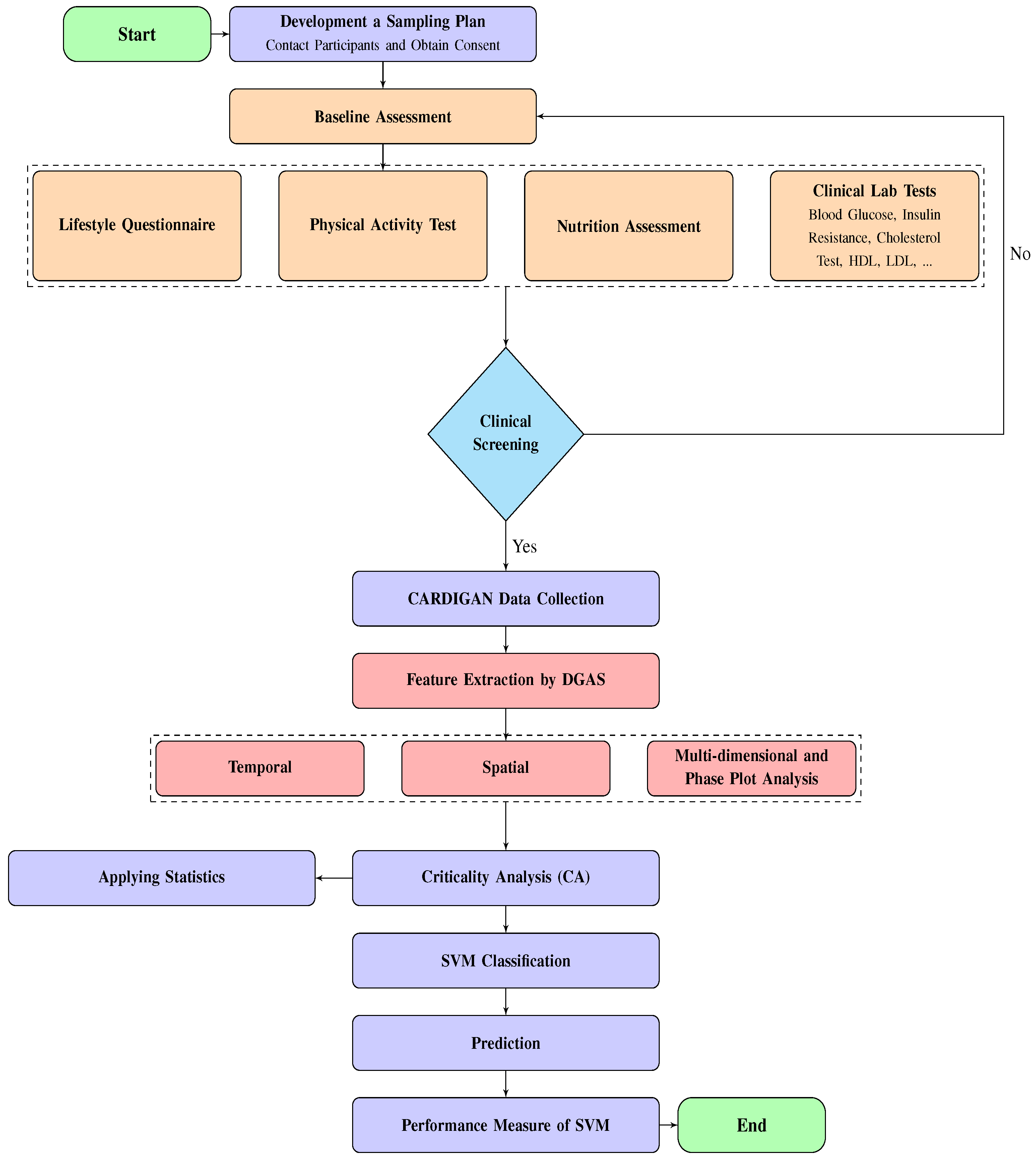
The proposed methodology for classifying human gait disorders includes a framework consisting of several key components, including data collection, data processing, feature extraction, and the use of the SVM technique. This methodology is illustrated in Figure 1.

6.1. Data Collection

In an effort to support the Criticality Analysis of Diabetic Gait in Children (CARDIGAN) project, a provisional clinical study was conducted at Mexico Children’s Hospital (MCH) between January 2019 and January 2020. Participants, who were at the early adolescence age and suffering from both Obesity and Diabetes, were offered the opportunity to participate in the study in accordance with the Newton Fund Grant Agreement. All participants provided informed consent prior to their involvement in the study.

The critical pathology characteristics of the participants were assessed by a medical professional prior to and during walking exercise. This assessment aimed to measure the participants’ ability to walk independently as their primary means of mobility, as well as to determine the underlying causes of their health conditions and their level of motivation to follow the program during the clinical study. Additionally, a healthy control group, free from peripheral injury or other conditions that may impede their mobility without the use of assistive devices, was also recruited to participate in the measurement of the trial.

For the clinical experiment, the participants, consisting of 50 individuals, were asked to walk back and forth along a 30-meter track on a flat surface over a period of 6 minutes and attempt to cover the distance in the minimum time possible while maintaining a brisk pace for the entire duration. Critical changes in walking control, stride frequency, and length of steps were observed as the participants changed speed, effectively stressing their mobility. The experiment was repeated after exposure to a 12-week complex dietary, psychological, and physical activity intervention aimed at improving fitness and reducing weight. Assessments were conducted immediately after the intervention, at 3 months, and again at 6 months as a follow-up.

The assessment was based on the use of an inertial measurement movement sensor (IMU), placed on the fourth lumbar vertebra located on the top left of the anatomical position of the lumber spine, known as the body Centre of Mass (CoM). The sensor was designed to be incredibly flexible, providing for mobility in many different planes including flexion, extension, side bending, and rotation. Gait analysis was conducted for participants using a standardised 6-meter test, wherein an IMU was attached to the lower back to capture triaxial accelerometer and gyroscope data at a frequency of 100 Hz. For individuals with DPN (Diabetic Peripheral Neuropathy), the assessment took place at OCDEM (Oxford Centre for Diabetes, Endocrinology, and Metabolism) in a dedicated obstacle-free corridor. The methodology employed for deriving gait parameters has been comprehensively described in previous studies [34,35,36,37]. The spatiotemporal parameters derived from the gait analysis included step time (in milliseconds), cadence (in steps per minute), stride length (in meters), and walking speed (in meters per second). Additionally, gait control parameters were calculated, which comprised beta (in degrees), SDa (in arbitrary units), SDb (in arbitrary units), ratio (in arbitrary units) [10], and walk ratio (in millimeters per steps per minute). These parameters have been identified as indicators of neuro motor control [38]. The dynamics of their walking activity were monitored using the Polar Team tracking system [39]. Under the rules of General Data Protection Regulation (GDPR), the collected CARDIGAN dataset has been anonymised and shared with Oxford Brookes University for research. The data underwent official approval procedures by the University Research Ethics Committee (UREC) before being analysed. The data was divided into three groups: Healthy controls, individuals with Obesity, and those with Diabetes. However, because of a lack of diabetic data points, they were not included in the analysis. Only 40 data points were used for the analysis, with 20 coming from the healthy control group and the remaining from the Obesity group.

6.2. Method for Analysing Gait and Extracting Features

The CARDIGAN dataset, which was collected utilising a 3-dimensional accelerometer, gyroscope, and magnetometer IMU sensor, was analysed utilising the DataGait Analysis Software (DGAS). Developed as a standalone software analysis package by the Movement Science Group at Oxford Brookes University using LabVIEW2011 (National Instruments, Ireland), the DGAS employs quaternion rotation matrices and double integration to transpose the accelerations frame of the

z -

axis from the object to the global system, thereby allowing for the measurement of translatory vertical CoM accelerations during walking and the achievement of a relative change in position. As referenced in [34] [39], the upward CoM measurements determine the global quality of human gait parameters. The DGAS extracts critical features of individuals’ gait for the purpose of classification. Biologically distinct masculine and feminine gait patterns can be distinguished through the use of spatiotemporal parameters, which describe the dynamics of human gait patterns at specific time points, as well as phase plot analysis, which allows for the discovery of variability in different gait pattern structures. DGAS extracts a total of 17 features from the raw sensory data of CARDIGAN, as listed in Table 1.

6.3. Representation of Gait Data Using Criticality Analysis

Criticality Analysis based on the RCC concept is a method used to represent complex multivariate data patterns in a simplified form, typically in the form of a phase plot portrait or manifold. This method involves analysing the data in multiple dimensions and identifying patterns or structures that are most critical to understanding the underlying dynamics of the system. 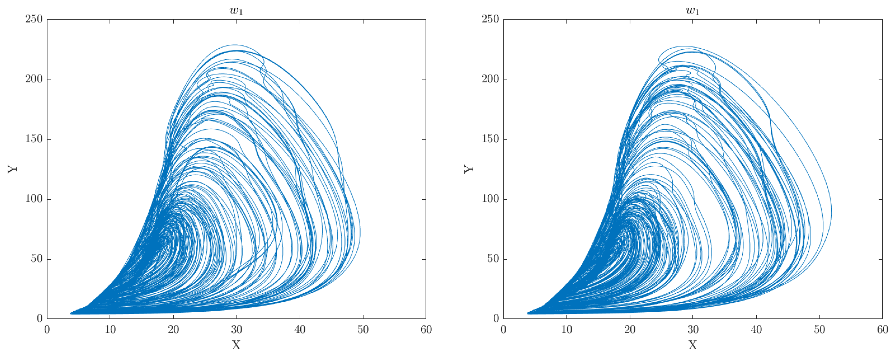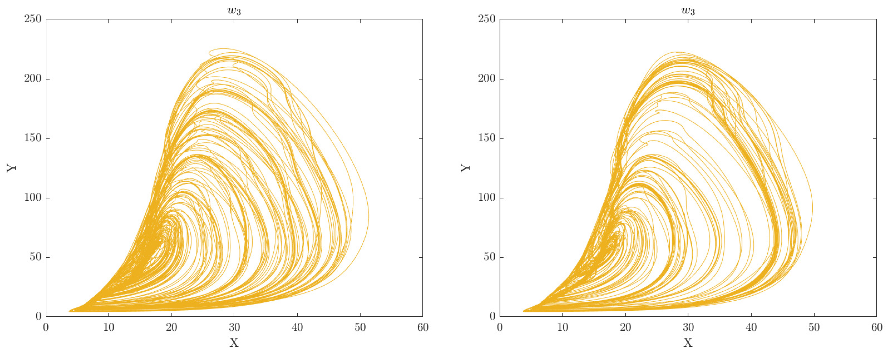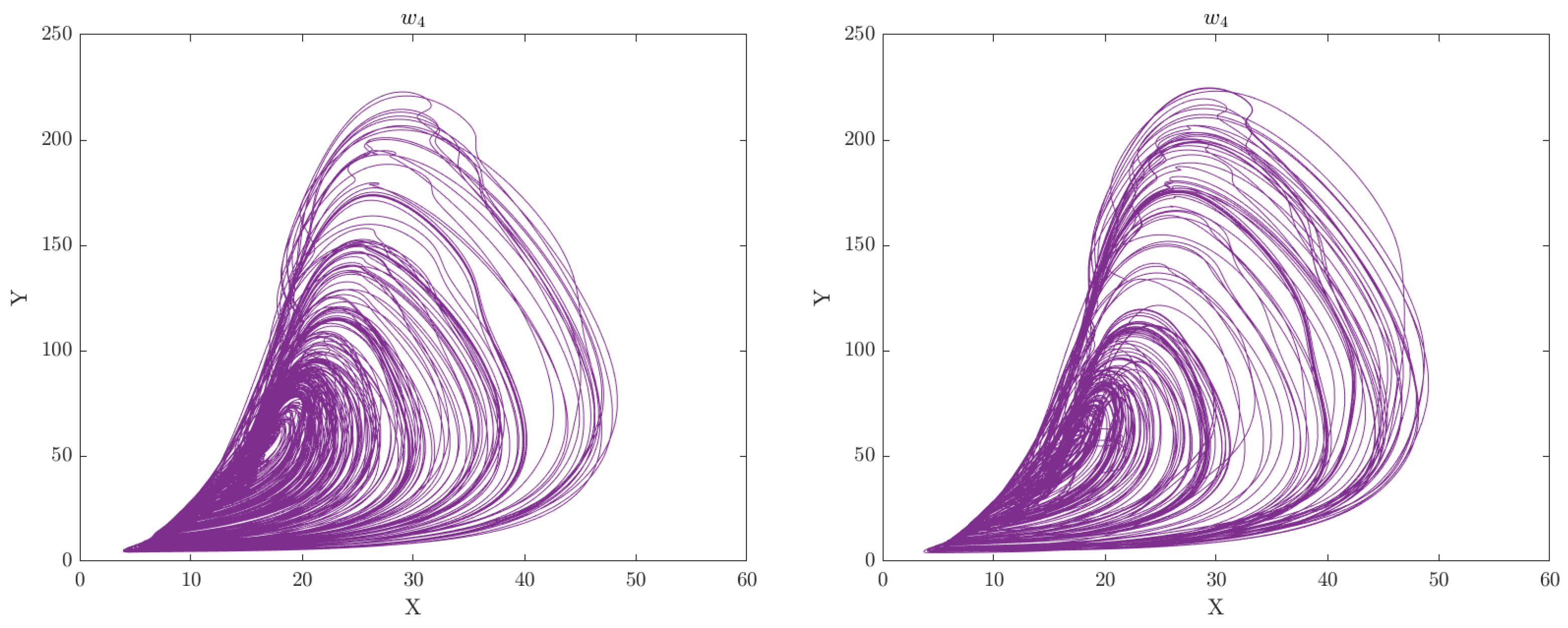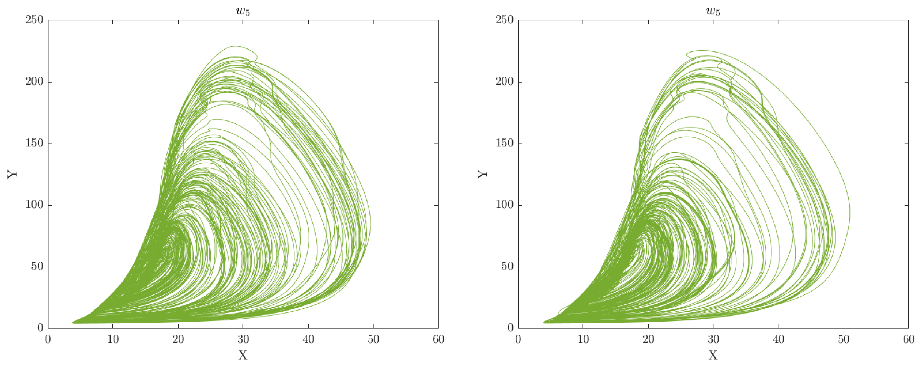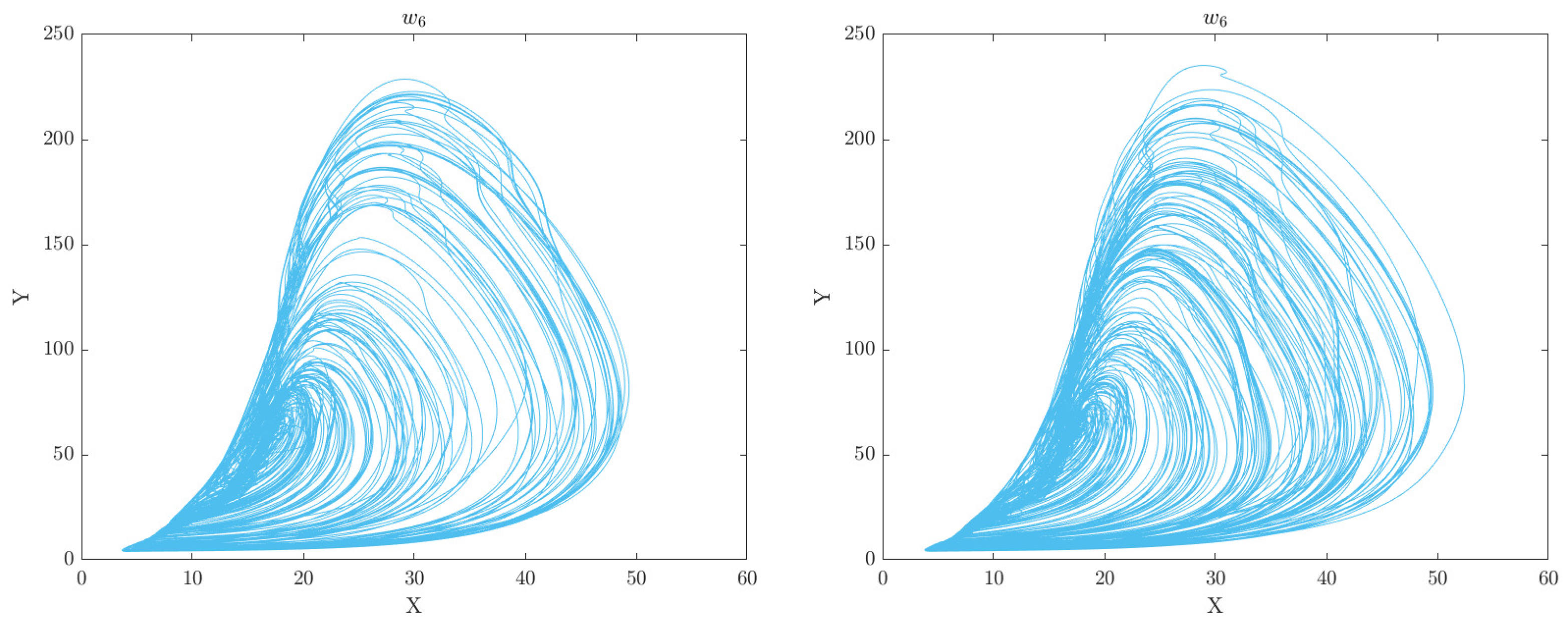The extracted features by DGAS can serve as perturbation inputs to the extended CA model represented by Equations 4 and 7, respectively. This can aid in gaining a deeper understanding of the underlying mechanisms and dynamics of the system under study. Through this analysis, we can gain insights into the intricate relationships between the various features and identify crucial patterns or structures that are vital for understanding the behavior of the motor system. The phase space plots of the CA data representation for the categorised groups of participants (Healthy Control and Obesity) during the 6 clinical weeks are displayed in Figure 2, Figure 3, Figure 4, Figure 5, Figure 6 and Figure 7 respectively.

The analysis of the CA phase plots, presented in Figure 2,Figure 3,Figure 4,Figure 5,Figure 6 and Figure 7, demonstrates that obese individuals exhibit a gait pattern that is slower and more labored in comparison to healthy individuals. The additional weight carried by obese individuals leads to increased stress on joints and muscles, resulting in stiffness during walking. Furthermore, obesity is associated with an increased risk of conditions such as joint pain and arthritis, which can contribute to stiffness in the gait. Conversely, healthy individuals display a gait pattern that is smooth and fluid with a narrower base of support and longer steps and have less stiffness in their walking. It is also important to note that the gait features depicted in these figures can have an impact on the network of coupled CA oscillators. The scaling of additive connectivity strength in response to external perturbations of gait can either enhance or hinder gait patterns. This is done to ensure that the input provided to each oscillator does not exceed a certain threshold and remains within the controlled domain.

6.4. Spatiotemporal Analysis of Gait Data

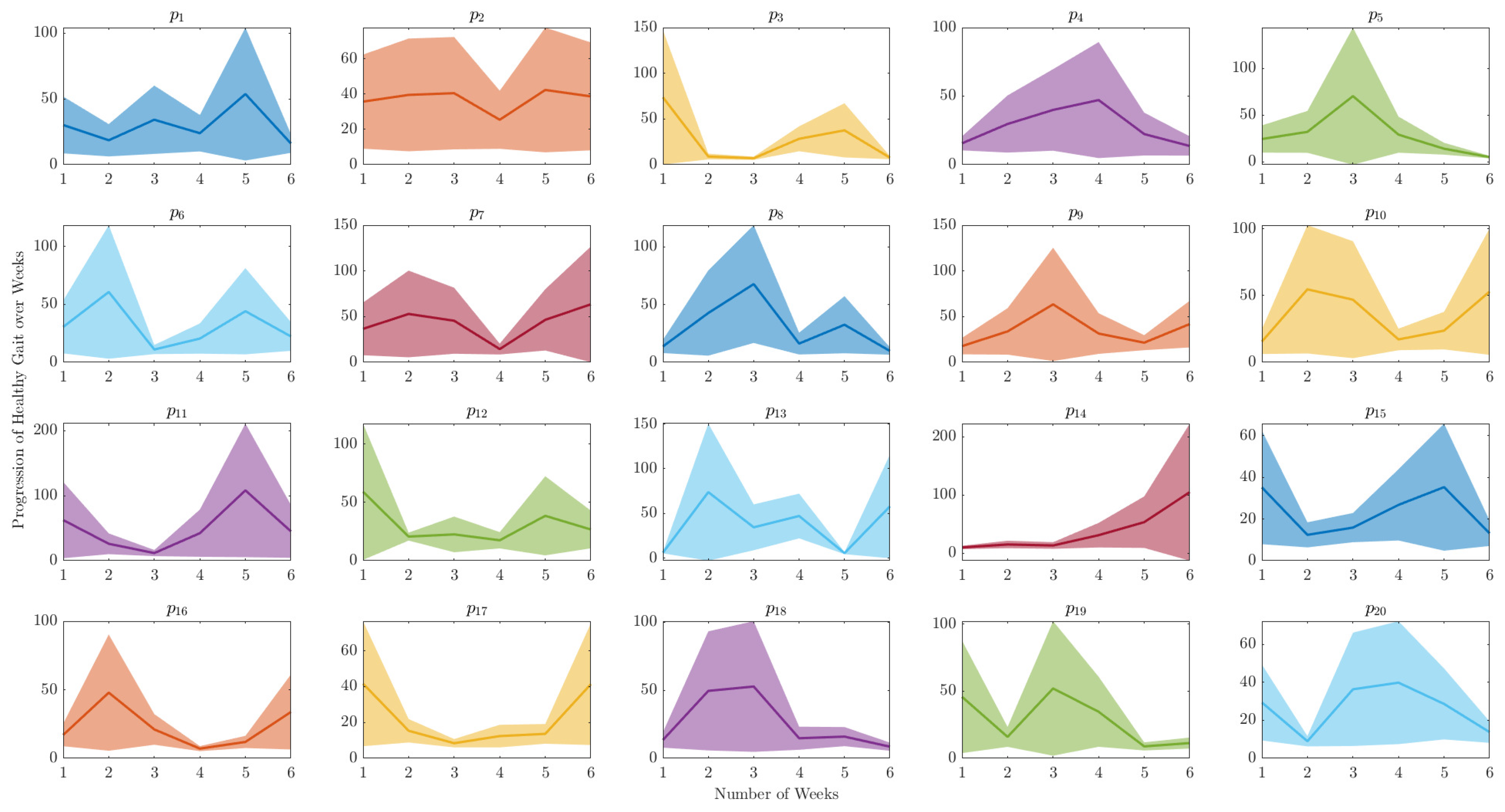
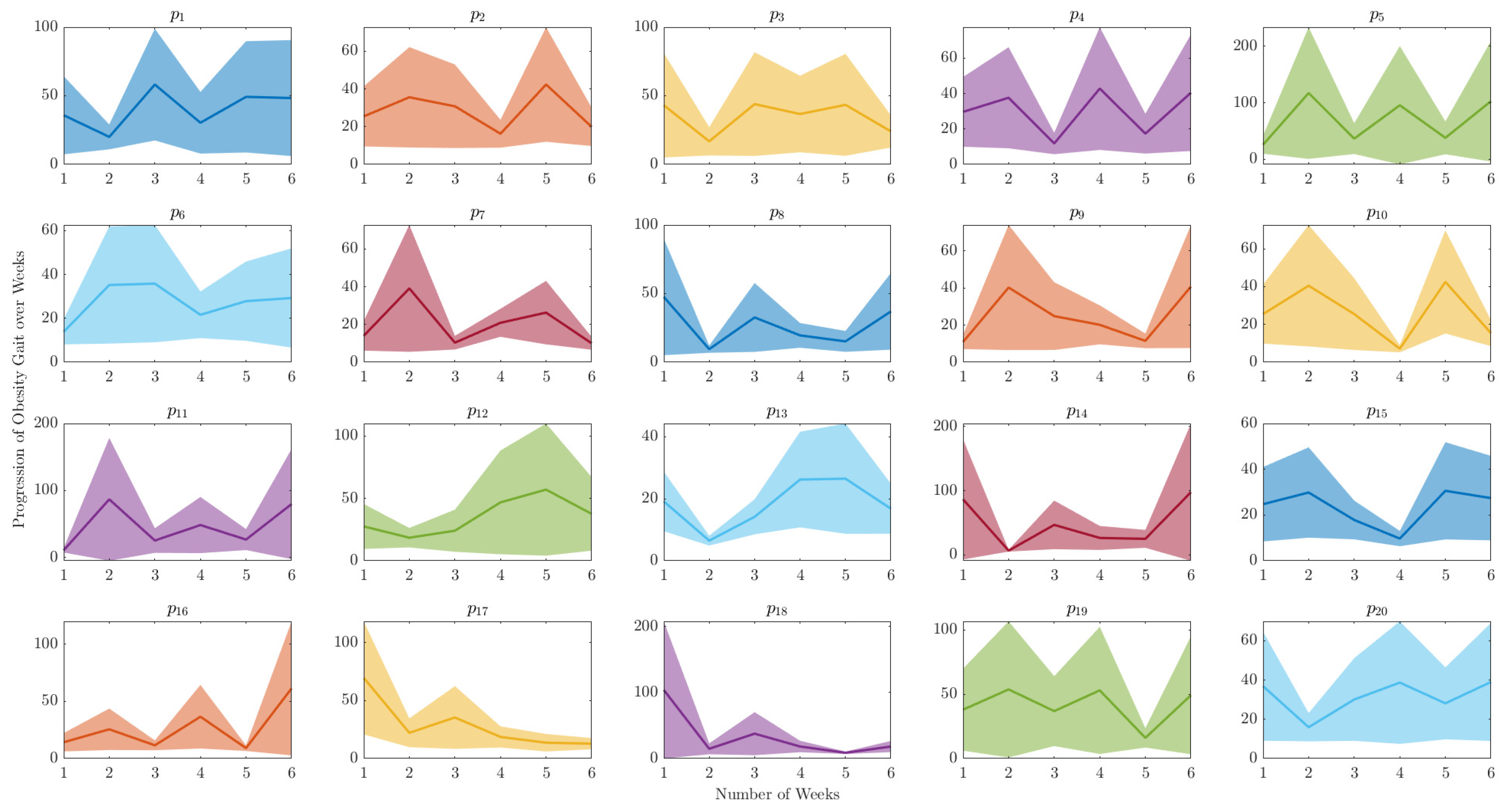
This section presents a comprehensive examination of spatiotemporal analysis of human gait data. The objective of this analysis is to gain a deeper understanding of the underlying mechanics of human walking and to detect any variations from normal gait patterns. A methodical analysis of the progression of gait over time was undertaken for both healthy control and obese participants by utilising a technique of extracting the peak value of each orbit of the phase plot for each clinical week. Consequently, a graphical representation of the progression of each participant was produced over the six-week period, enabling an in-depth understanding of the evolution of gait patterns as shown in Figure 8 and Figure 9.

The Figure 8 and Figure 9 depict the range of variability in human gait progression over a 6-week period. They indicate the level of uncertainty surrounding the average gait progression for a group of individuals, and can be used to detect notable changes or trends in gait progression during the clinical examination study. Additionally, these figures compare the gait progression between healthy control and obesity groups, as well as to monitor an individual’s progress in terms of walking patterns over time.

6.5. SVM Classifier

The proposed Support Vector Machine (SVM) model capitalises on the utilisation of the Kernel property outlined in Section 5, owing to its capability of converting this nonlinear dynamic gait data into a novel feature space, thereby streamlining the classification process. The controlled CA model extracts salient features, represented by f of Equation 5 on the x-axis and m of Equation 4 on the y-axis, that serve as inputs for the SVM algorithm, enabling the assessment of classification performance under varying settings. The proposed SVM classifier underwent rigorous training and testing utilising these extracted features, specifically for both the healthy control and obese groups. The primary objective of this experiment was to evaluate the capacity of the SVM to discern gait patterns between the two groups. Algorithm 1 outlines the implementation procedures of the proposed SVM algorithm.

Algorithm 1:Pseudocode of SVM Implementation

1:: Input: Given a training set $Ω = (x_{i}, y_{i}) :$ $x_{i} \in R^{m},$ $y_{i} \in \{- 1, + 1\},$ $i = \{1, 2, . . ., N\}$ and testing data set $x \in R^{m}$ .
2:: Output: Predict subjects label for testing data $x$ .
3:: Select a regularisation parameter C such that $C > 0$ and choose an appropriate kernel width control variable $σ$ for validation.
4:: Compute Gaussian Kernel RBF $κ (x_{i}, x_{j}) = exp (\frac{- {∥ x_{i} - x_{j} ∥}^{2}}{2 σ^{2}})$ .
5:: Solve the kernalised optimisation problem in equation 15 using CVX optimisation solver [40] in MATLAB.
6:: Obtain optimal value of $β$ in equation 15 and the bias b in equation 13.
7:: Predict labels for testing data $x$ .
8:: Obtain performance measure (Confusion Matrix, Accuracy, Receiver Operating Characteristics (ROC) Curve.

6.6. SVM Model Training

The CARDIGAN dataset for this study comprises 20 data points per gait subject, resulting in a total of 40 data samples for both the healthy control and obesity subjects. The training and testing of the Kernel SVM classifier employed a

50 %

splitting ratio. In preparation for the SVM algorithm training process, all CA gait features were normalised using the z-score method, resulting in a zero mean and unity standard deviation for the data samples. The Kernel SVM algorithm, as outlined in Algorithm 1, was implemented utilizing MATLAB to examine the influence of Kernel characteristics, specifically the regularisation parameter C and control width

σ

, on the classification performance of gait data. The generalisation performance of the trained Kernel SVM was evaluated by measuring the prediction accuracy for each model, analysing the confusion matrix, plotting the Receiver Operating Characteristics (ROC) curve, and computing the area under the ROC curve. These evaluations are discussed in the subsequent sections of this paper.

6.7. Confusion Matrix

In a binary classification problem, the dataset labels can be dichotomised into either positive or negative outcomes. The decision made by the SVM classifier can be represented by a structured contingency table known as a confusion matrix. This matrix comprises actual and predicted binary classification information, which can be utilised to evaluate the ability of the SVM classification algorithm to distinguish between various categories. The confusion matrix comprises four principal characteristics [41]:

The terms True Positive

(T P)

, False Positive

(F P)

, True Negative

(T N)

, and False Negative

(F N)

are used to evaluate the performance of the Kernel SVM classifier. Specifically,

True Positive $(T P)$ refers to the number of positive data samples (healthy control participants) that are accurately classified as positive (healthy).
False Positive $(F P)$ refers to the number of negative data samples (obese participants) that are incorrectly classified as positive (healthy).
True Negative $(T N)$ refers to the number of negative data samples (obese individuals) that are accurately classified as negative (obese).
False Negative $(F N)$ refers to the number of positive data samples (healthy control) that are inaccurately classified as negative (obese individuals).

These terms provide insight into the classifier’s ability to distinguish between the two gait categories and inform the overall evaluation of the model’s performance.

In addition to the terms True Positive

(T P)

, False Positive

(F P)

, True Negative

(T N)

, and False Negative

(F N)

, various performance metrics are used to evaluate the classifier’s performance. These metrics include accuracy, precision, F

_{1} -

Score, Recall or Sensitivity or True Positive Rate

(T P R)

, Specificity or True Negative Rate

(T N R)

, and False Positive Rate

(F P R)

. These metrics are calculated based on the previously mentioned

T P

F P

T N

, and

F N

values. Their definitions are as follows:

Accuracy: The prediction accuracy of the Kernel SVM classifier is represented as the overall rate of correct predictions. Mathematically, it is expressed as the ratio of correctly classified labels $(T P + T N)$ to the total number of data samples $(T P + T N + F P + T N)$ . This value is determined by the following equation:

$A c c u r a c y = \frac{T P + T N}{T P + T N + F P + T N} .$
Precision: This metric used to evaluate the classifier’s ability to accurately predict positive labels with normal walk status is the ratio of correctly predicted labels to the total labels predicted to have a normal walk condition. This measurement is quantified using the following expression:

$P r e c i s i o n = \frac{T P}{T P + F P} .$
Recall (TPR): It is quantified as the ratio of correctly predicted positive labels corresponding to normal gait among all data samples of normal gait. It is calculated using the following expression:

$R e c a l l = \frac{T P}{T P + F N} .$
$F_{1} -$ Score: The F measure is a metric that maintains a balance between precision and recall, it is computed as:

$F_{1} - S c o r e = \frac{2 \times P r e c i s i o n}{P r e c i s i o n + R e c a l l} .$
True Negative Rate (TNR): The Specificity metric is defined as the proportion of correctly classified negative labels among all data samples associated with the strapped walk condition. It is mathematically formulated as:

$T N R = \frac{T N}{T N + F P} .$
False Positive Rate (FPR): The error rate is computed as the proportion of incorrectly labeled strapped walk samples among all strapped data samples. It is quantified as follows:

$F P R = \frac{F P}{F P + T N} .$

The metrics outlined above serve to evaluate the ability of the proposed SVM algorithm to detect irregular gait patterns associated with different individuals. The performance metrics of the SVM classifier for each individual at specific values of the regularization parameter

C = (0.1, 1, 10)

are summarised in Appendix A. The primary metric for validation, which provides insight into the overall performance of the SVM classifier, is accuracy. The accuracy of the classifier is affected by the values of

σ

and C. In general, the optimal performance was achieved when

σ =

0.1 and 1.

7. Experiment Results

To better evaluate the effectiveness of the proposed methodology outlined above, the following performance measures are followed:

In this section, we present the findings of our experimental investigation, which encompasses the performance of the SVM classifier in identifying gait patterns for both healthy control and obese groups. Additionally, we examine the impact of various Kernel SVM model parameters on the classification performance. A comprehensive analysis of the generalization performance of the trained Kernel SVM is also presented, including Receiver Operating Characteristics (ROC) curve, the area under the ROC curve, and the SVM decision classification boundary. The results demonstrate the potential of using SVM in combination with a controlled CA model for accurate detection of gait patterns associated with healthy controls and individuals with obesity.

7.1. Receiver Operating Characteristic (ROC) Curve

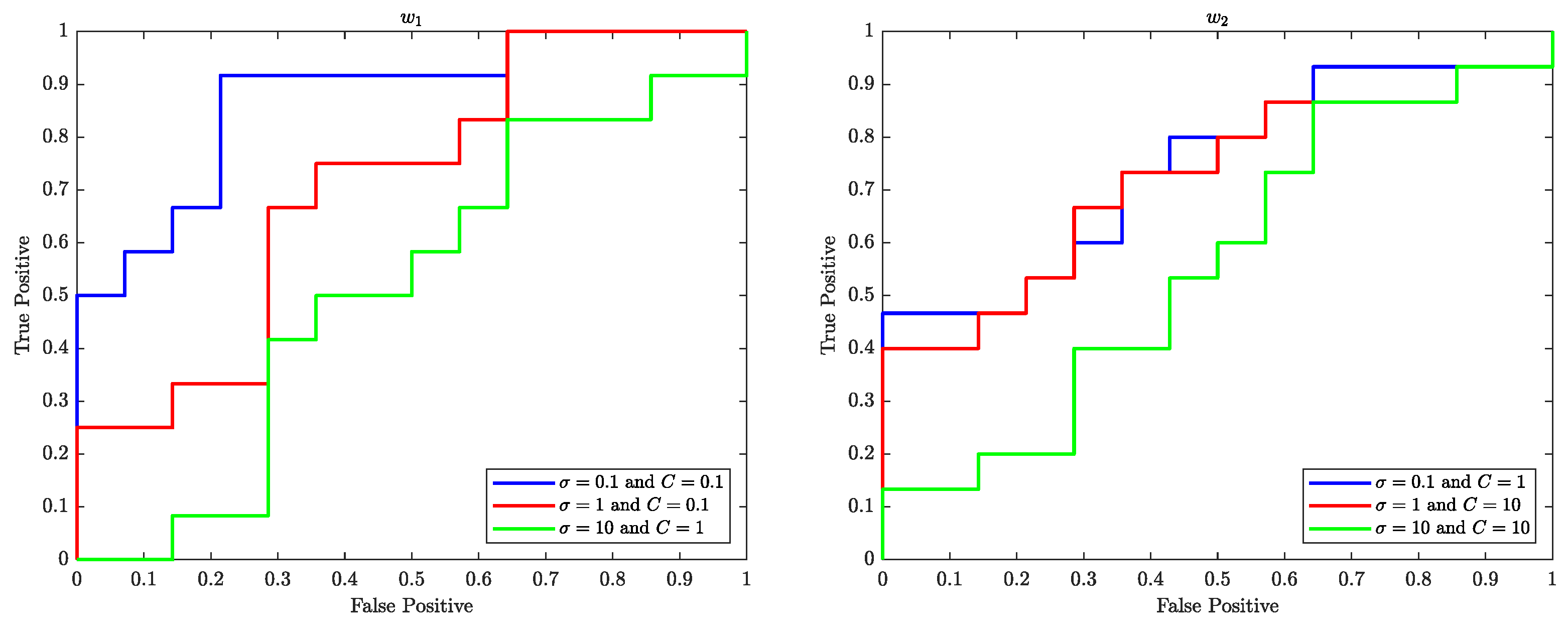
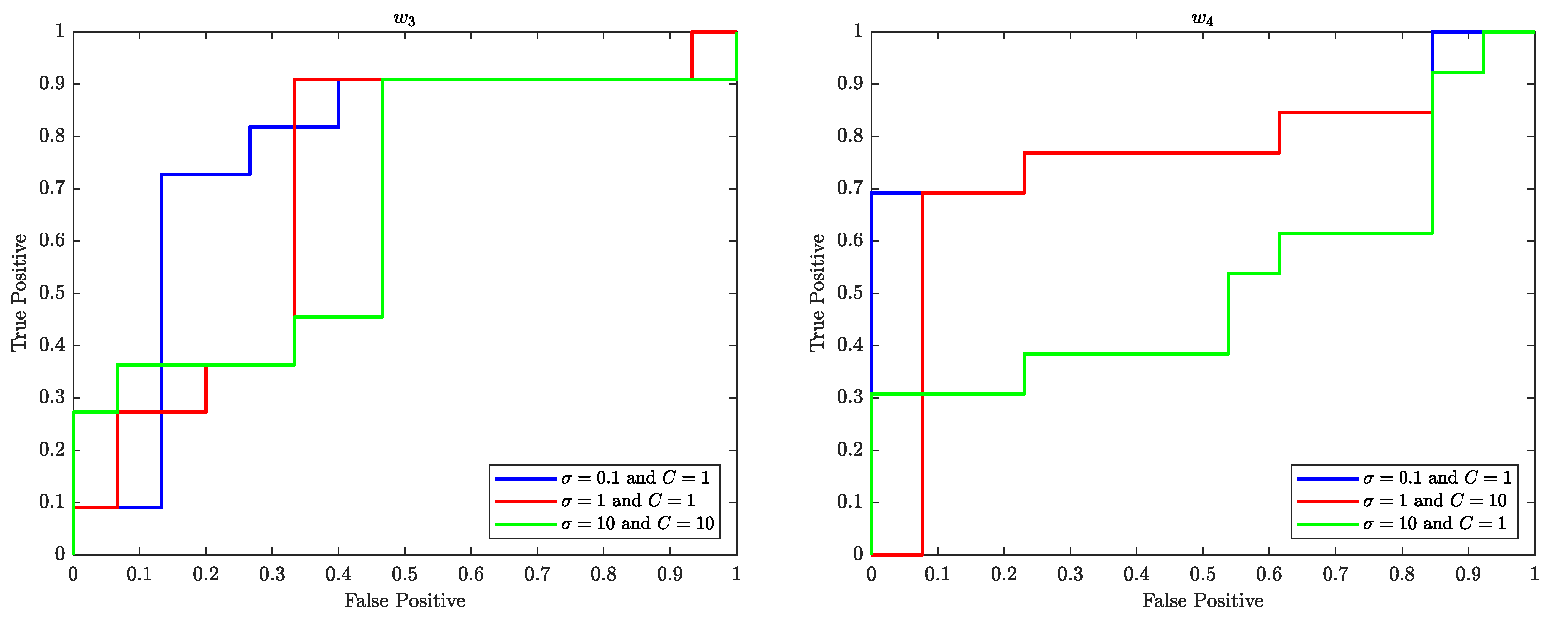
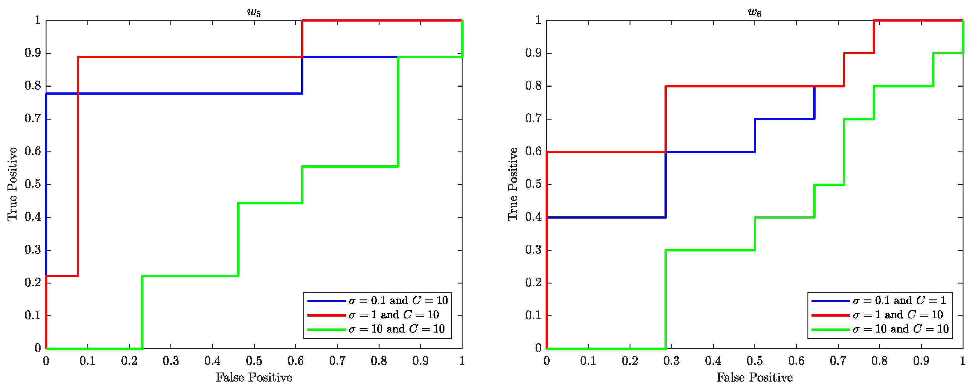
The Receiver Operating Characteristics (ROC) curve is a graphical representation of the performance of a binary classifier system as the discrimination threshold is varied. In the context of SVM, the ROC curve is used to evaluate the performance of the SVM classifier in classifying data samples into two different classes. The ROC curve plots the true positive rate (TPR) (sensitivity) against the false positive rate (FPR) (

\approx 1 - T N R

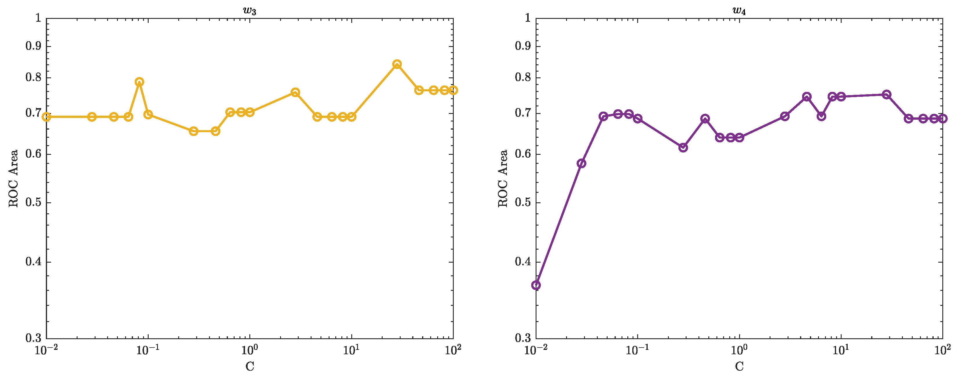
) at various threshold settings. Figure 10– Figure 12 illustrate the ROC curves for the best pair of

σ

and C values that satisfy the highest accuracy during the entire trial period.

The ROC plots (Figure 10– Figure 12) show that, in the context of SVM, the parameter C controls the trade-off between maximising the margin and minimising the misclassification error. When the value of C is smaller, such as

C = 0.1

, the margin becomes wider, but there are more instances of misclassifications. Conversely, a larger value of C, such as

C = 10

, leads to a narrower margin, but with a reduced number of misclassifications.

The parameter

σ

is used to control the width of the Kernel Gaussian function that is used to map the input data into a higher dimensional space, where a linear boundary can be found. A larger value of

σ

results in a wider Gaussian function, which leads to a softer decision boundary and a higher bias, while a smaller value of

σ

results in a narrower Gaussian function, which leads to a harder decision boundary and a higher variance.

When

σ

is small, the decision boundary is more sensitive to the input data, which can lead to overfitting. On the other hand, when

σ

is large, the decision boundary is less sensitive to the input data, which can lead to underfitting. Therefore, the value of

σ

has an impact on the generalisation performance of the SVM.

A good value for C and

σ

are the one that balance the trade-off of bias and variance, that is a good balance between overfitting and underfitting.

The ROC curves shown in Figure 10– Figure 12 performed well with

σ = 0.1

and 1 for various values of C of the SVM are likely because the classifier is able to find a good balance between overfitting and underfitting by adjusting the value of C and

σ

which in turn results in a good performance.

7.2. The Area Under the Curve (AUC)

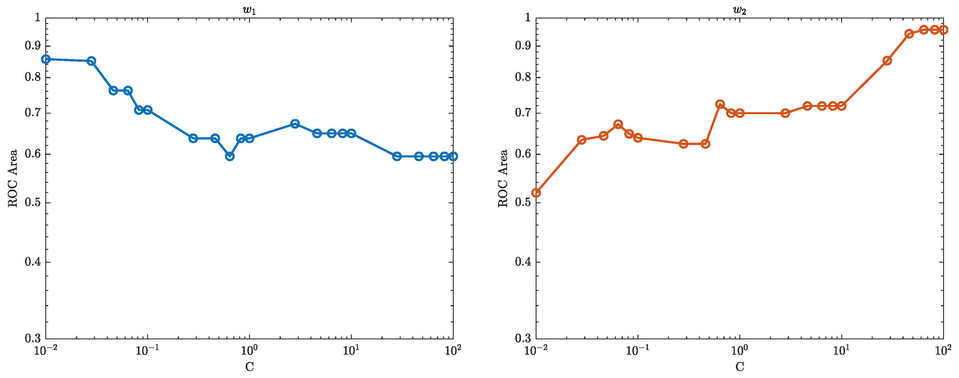
The area under the ROC curve, also known as the AUC (Area Under the Curve), is a measure of the performance of a binary classifier. In the context of SVM, the AUC represents the ability of the classifier to distinguish between the positive and negative classes. A higher AUC value indicates that the classifier is able to correctly classify more instances of the positive class as positive, while also correctly classifying more instances of the negative class as negative. An AUC of 1.0 represents a perfect classifier, while an AUC of 0.5 represents a classifier that performs no better than random guessing.

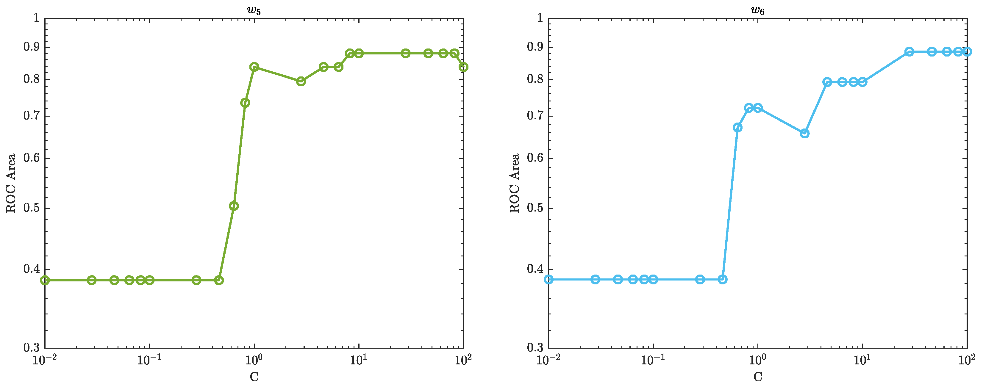
Figure 13– Figure 15 show how the performance of the SVM model changes as the regularisation parameter strength C is varied. The regularisation parameter C controls the trade-off between maximising the margin (the distance between the decision boundary and the closest training instances) and minimising the classification error. When C is small, the model will focus more on maximising the margin, which can lead to a simpler decision boundary but also a higher classification error. As C is increased, the model will focus more on minimising the classification error, which can lead to a more complex decision boundary but also lower classification error.

From Figure 13– Figure 15, if the AUC increases as C increases, it means that the model’s performance is improving as the regularisation strength C increases. This may suggest that the model was underfitting the data when C was small and that increasing the regularisation strength helped to improve the model’s performance. On the other hand, if the AUC decreases as C increases, it means that the model’s performance is worsening as the regularisation strength increases. This may suggest that the model was overfitting the data when C was small and that increasing the regularisation strength C caused the model to become too simplistic and lose important information from the data.

The optimal value of C is where the AUC is the highest, this is the sweet spot where the model is able to balance the trade-off between maximising the margin and minimising the classification error in a way that leads to the best classification performance.

7.3. The Classification Decision Boundary of SVM

The decision boundary of an SVM classifier is determined by the support vectors, which are the data points closest to the boundary. The parameters C and

σ

, also known as the regularisation and kernel parameters respectively, control the width of the margin and the shape of the decision boundary. For instance, When

σ

is set to 0.1 and C is set to 1, the decision boundary will be complex and more influenced by the individual data points. The width of the margin will be relatively small and the classifier will be more sensitive to the presence of outliers, as the algorithm tries to minimise misclassification errors. Moreover, When

σ

is set to 0.1 and C is set to 10, the decision boundary will be even more complex as C has a greater influence on the decision boundary. The width of the margin will be even smaller and the classifier will be even more sensitive to outliers. Furthermore, When

σ

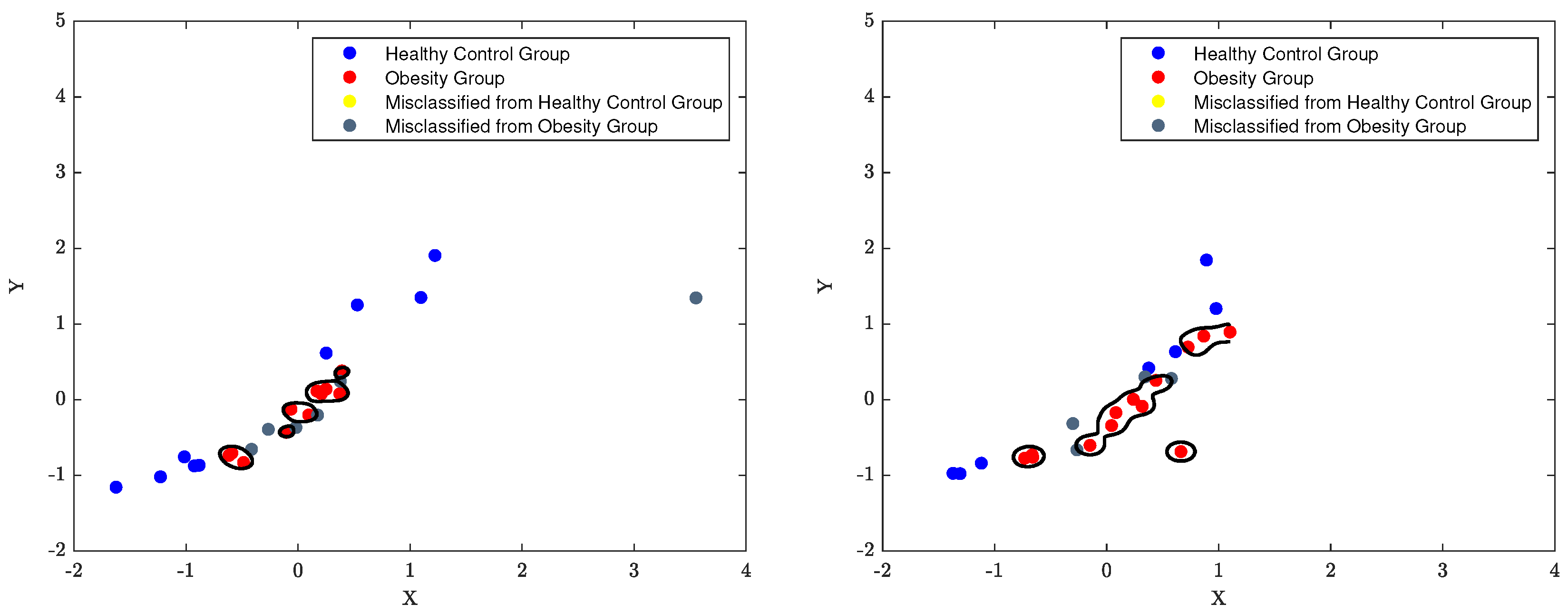
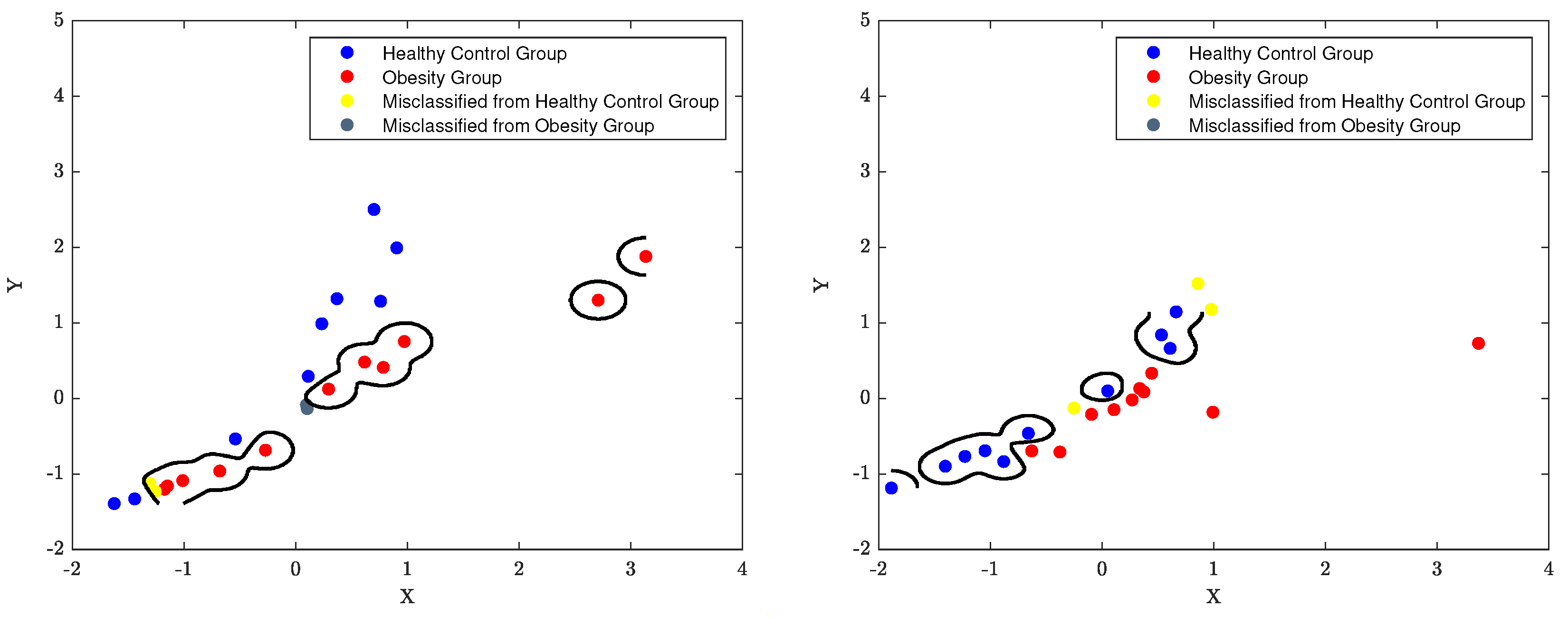
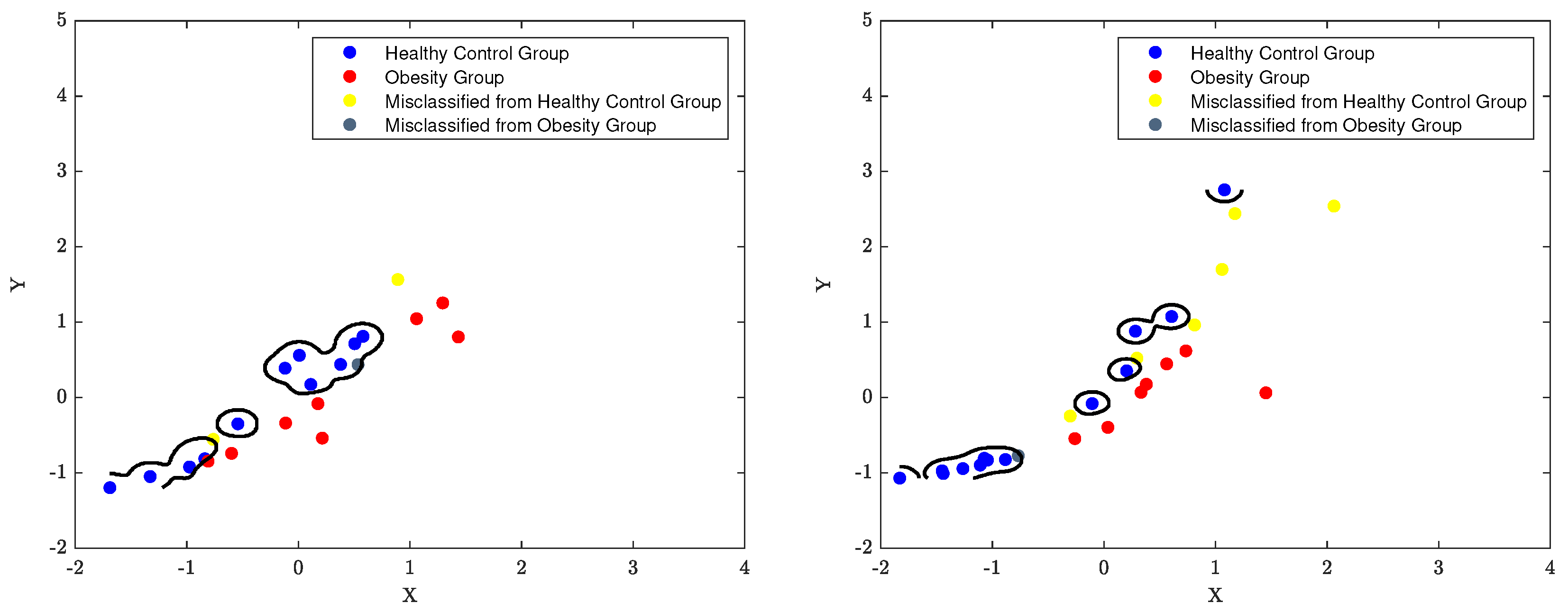
is set to 0.1 and C is set to 0.1, the decision boundary will be relatively simple as C has a much smaller influence on the decision boundary. The width of the margin will be relatively large and the classifier will be less sensitive to outliers. The classification boundaries of the SVM model are depicted in Figure 16 to Figure 18 using the best classification parameters, enabling the model to accurately categorise participants into the appropriate group.

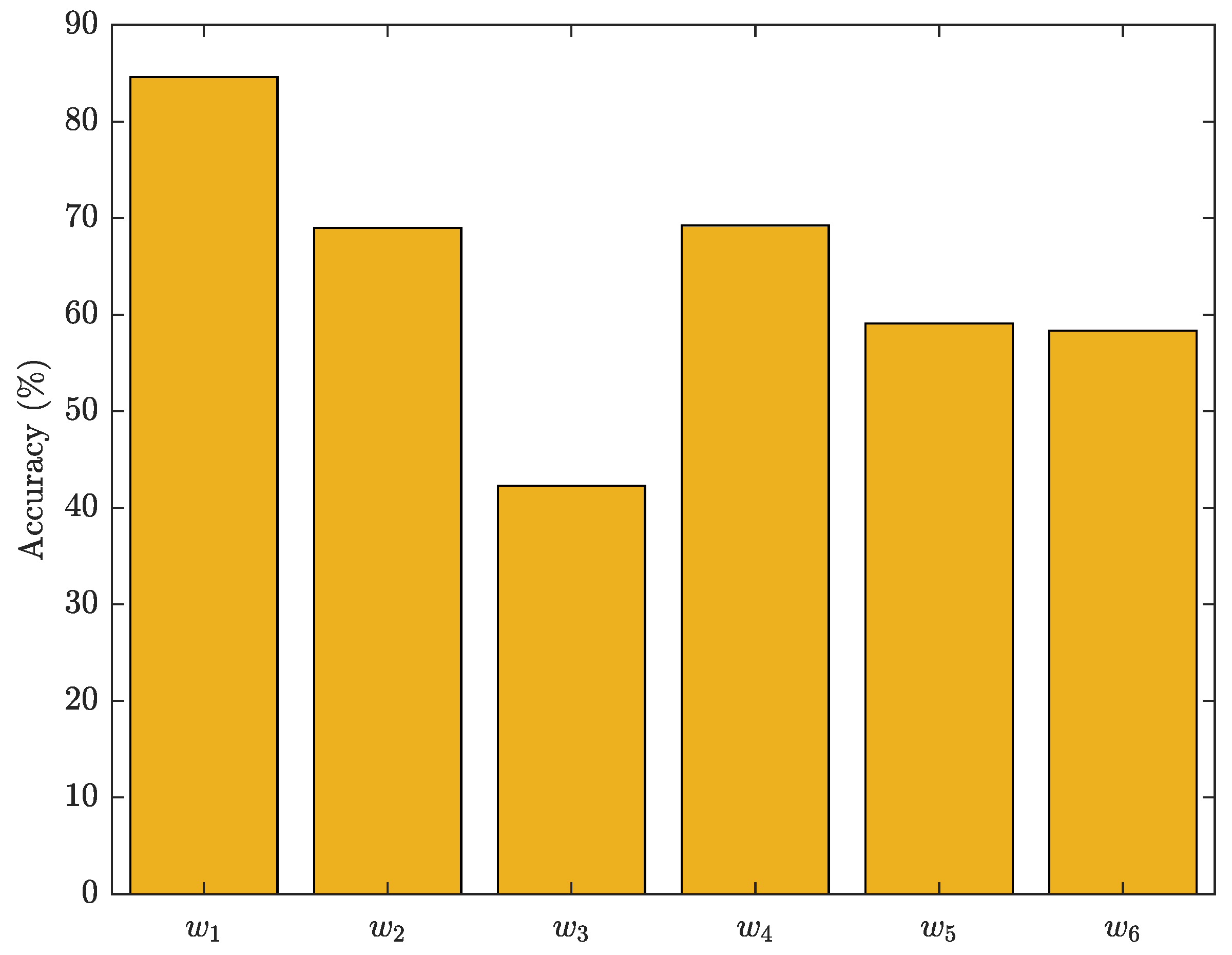
The overall performance of the proposed SVM model was evaluated in Figure 19, where the best classification parameters (

σ = 0.1

and

C = 0.1

) result in the optimal generalisation performance. The 6-week evaluation of the SVM shows fluctuating accuracy in classifying participants into the healthy control and obesity groups. A high accuracy reflects consistent participant characteristics, facilitating accurate classification by the SVM, whereas a low accuracy indicates high variability in participant characteristics, making classification challenging. In individuals with diabetes, the influence of various factors, including walk speed, affects the results depicted in Figure 19. The figure demonstrates that the highest accuracy is observed during the initial week, but experiences a significant decline in the third week. Subsequently, there is a slight improvement in the fourth week, followed by further declines in the fifth and sixth weeks. The fluctuation in the accuracy of the SVM model during the 6 weeks period, despite the uniform diet and exercise regimen followed by the participants, could be attributed to various reasons such as variations in compliance levels, where some participants may have been more diligent in adhering to the regimen than others, leading to different classifications into healthy control or obesity groups. Other factors include individual differences such as genetics, medical history, and personal habits, measurement inaccuracies, and changes in any of the systems (metabolic, neuromuscular, cardiovascular) altering the participants characteristics over time, even when following the prescribed diet and exercise regimen. Participants stress levels or health status could impact their classification as it could alter variables affecting their gait and hence membership into healthy control or obesity groups.

8. Discussion

The primary objective of this study was to assess the effectiveness of the criticality analysis technique in identifying gait irregularities among pediatric individuals afflicted with metabolic disorders, specifically obesity. As a result, the research presented in this paper has successfully accomplished its principal aim. The SVM classifier with the CA system yielded a detection rate of 78.2% to 90%, indicating that CA is an effective approach for representing multivariate data and reducing dimensionality. Interestingly, we observed a reduction in accuracy over the six-week training period. This finding suggests that as young individuals improved their fitness and walked faster, the classification patterns underwent alterations, which varied between individuals. Further studies should explore the relationship between these classification changes in individuals and both fitness and metabolic variables.

The effectiveness of the proposed approach was assessed using the confusion matrix, receiver operating characteristics (ROC), and area under the ROC metrics. The combination of the CA method and the kernelised properties of the SVM model produced better results. These findings suggest that the proposed SVM model with CA support can be a reliable tool for identifying dynamic disruptions in biological data patterns, providing great potential for clinical diagnosis and rehabilitation.

The limited sample size of the CARDIGAN dataset, which consisted of only 40 samples, used in this study, could impact the performance of the SVM classification process. However, our previous research [3] applied the CA methodology with a larger dataset of 6000 data samples and achieved an impressive 94% accuracy.

Despite this constraint, our results hold promise and offer various opportunities for further exploration, such as investigating how the CA method can be combined with other machine learning models to increase accuracy and performance. This could involve incorporating CA with other unsupervised methods such as dimensionality reduction, or with supervised methods such as neural networks or regression. The outcomes from CA can also serve as inputs or features for other models. The objective of this integration is to harness the strengths of different techniques and overcome their limitations.

9. Conclusions

The criticality analysis approach presented in this paper has been demonstrated as a valuable tool for representing gait data and highlighting medical conditions. The variability and detection of changes over time are interesting, as they highlight the potential of the system to determine changes in various systems, such as cardiovascular and metabolic responses to interventions. The detection of gait disorders is a complex and interdisciplinary process that can benefit from the integration of advanced technologies. By utilising a combination of criticality analysis and supervised machine learning methods, such as the SVM classifier, this research has the potential to significantly advance the field of gait analysis and lead to more precise diagnoses, improved patient outcomes, and empowered individuals in managing their health.

Author Contributions

Conceptualisation, S.E.; methodology, S.E. and T.V.o.S.; validation, S.E.; formal analysis, S.E.; investigation, S.E.; data curation, H.D., J.C., A.A., C.M., M.MB., S.L., S.VC., M.J.A., and D.F.; writing—original draft preparation, S.E.; writing—review and editing, S.E. and T.V.o.S.; visualisation, S.E.; supervision, T.V.o.S. All authors have read and agreed to the published version of the manuscript.

Funding

This work was supported by a Newton Fund Institutional Links grant, (grant ID: 432368181), under the Newton-Mosharafa Fund partnership between the United Kingdom and Mexico. The grant was funded by the UK Department for Business, Energy and Industrial Strategy (BEIS) and delivered by the British Council. The funding supported collaboration activities between Oxford Brookes University and Hospital Infantil de Mexico Federico Gomez under the Newton Institutional Links program administered by the British Council.

Institutional Review Board Statement

Not applicable.

Informed Consent Statement

Not applicable.

Data Availability Statement

In accordance with the General Data Protection Regulation (GDPR) guidelines, the database utilised in this study is maintained in a confidential and secure manner within the purview of the Faculty of Health and Life Sciences at Oxford Brookes University. Owing to privacy considerations, access to the dataset is restricted to authorised personnel only.

Acknowledgments

The authors gratefully acknowledge the support provided by the British Council under the Newton Fund Institutional Links program for making this collaboration possible. We also acknowledge our institutional partners Oxford Brookes University and Hospital Infantil de Mexico Federico Gomez for their support and contribution.

Conflicts of Interest

The authors declare no conflict of interest.

Appendix A

Table A1. SVM Classification Results of

w_{1}

Table A1. SVM Classification Results of

w_{1}

Performance	$σ = 0.1$
	$C = 0.1$	$C = 1$	$C = 10$
TP	11	14	14
FP	1	5	5
FN	3	0	0
TN	11	7	7
FPR	0.083	0.416	0.416
Precision	0.916	0.736	0.736
Recall	0.785	1	1
F $1 -$ Score	0.846	0.848	0.848
Specificity	0.916	0.583	0.583
AROC	0.875	0.755	0.755
Accuracy $(%)$	84.61	80.76	80.76
Performance	$σ = 1$
	$C = 0.1$	$C = 1$	$C = 10$
TP	14	14	14
FP	9	10	9
FN	0	0	0
TN	3	2	3
FPR	0.75	0.833	0.75
Precision	0.608	0.583	0.608
Recall	1	1	1
F $1 -$ Score	0.756	0.736	0.756
Specificity	0.25	0.166	0.25
AROC	0.708	0.636	0.648
Accuracy $(%)$	65.38	61.53	65.38
Performance	$σ = 10$
	$C = 0.1$	$C = 1$	$C = 10$
TP	0	14	14
FP	0	12	12
FN	14	0	0
TN	12	0	0
FPR	0	1	1
Precision	0	0.538	0.538
Recall	0	1	1
F $1 -$ Score	0	0.7	0.7
Specificity	1	0	0
AROC	0.511	0.511	0.511
Accuracy $(%)$	46.15	53.84	53.84

Table A2. SVM Classification Results of

w_{2}

Table A2. SVM Classification Results of

w_{2}

Performance	$σ = 0.1$
	$C = 0.1$	$C = 1$	$C = 10$
TP	5	13	13
FP	0	8	8
FN	9	1	1
TN	15	7	7
FPR	0	0.533	0.533
Precision	1	0.619	0.619
Recall	0.357	0.928	0.928
F $1 -$ Score	0.526	0.742	0.742
Specificity	1	0.466	0.466
AROC	0.714	0.742	0.742
Accuracy $(%)$	68.96	68.96	68.96
Performance	$σ = 1$
	$C = 0.1$	$C = 1$	$C = 10$
TP	13	14	14
FP	10	10	9
FN	1	0	0
TN	5	5	6
FPR	0.667	0.667	0.6
Precision	0.565	0.583	0.608
Recall	0.928	1	1
F $1 -$ Score	0.702	0.736	0.756
Specificity	0.333	0.333	0.4
AROC	0.638	0.7	0.719
Accuracy $(%)$	62.06	65.51	68.96
Performance	$σ = 10$
	$C = 0.1$	$C = 1$	$C = 10$
TP	0	13	14
FP	0	13	13
FN	14	1	0
TN	15	2	2
FPR	0	0.866	0.866
Precision	0	0.5	0.518
Recall	0	0.928	1
F $1 -$ Score	0	0.65	0.682
Specificity	1	0.133	0.133
AROC	0.519	0.5	0.557
Accuracy $(%)$	51.72	51.72	55.17

Table A3. SVM Classification Results of

w_{3}

Table A3. SVM Classification Results of

w_{3}

Performance	$σ = 0.1$
	$C = 0.1$	$C = 1$	$C = 10$
TP	0	11	11
FP	0	3	3
FN	15	4	4
TN	11	8	8
FPR	0	0.272	0.272
Precision	0	0.785	0.785
Recall	0	0.733	0.733
F $1 -$ Score	0	0.758	0.758
Specificity	1	0.727	0.727
AROC	0.690	0.769	0.769
Accuracy $(%)$	42.30	73.07	73.07
Performance	$σ = 1$
	$C = 0.1$	$C = 1$	$C = 10$
TP	10	14	15
FP	5	9	11
FN	5	1	0
TN	6	2	0
FPR	0.454	0.818	1
Precision	0.667	0.608	0.576
Recall	0.667	0.933	1
F $1 -$ Score	0.667	0.736	0.731
Specificity	0.545	0.181	0
AROC	0.696	0.703	0.690
Accuracy $(%)$	61.53	61.53	57.69
Performance	$σ = 10$
	$C = 0.1$	$C = 1$	$C = 10$
TP	0	0	12
FP	0	0	7
FN	15	15	3
TN	11	11	4
FPR	0	0	0.636
Precision	0	0	0.631
Recall	0	0	0.8
F $1 -$ Score	0	0	0.705
Specificity	1	1	0.363
AROC	0.690	0.690	0.660
Accuracy $(%)$	42.30	42.30	61.53

Table A4. SVM Classification Results of

w_{4}

Table A4. SVM Classification Results of

w_{4}

Performance	$σ = 0.1$
	$C = 0.1$	$C = 1$	$C = 10$
TP	5	13	13
FP	0	5	5
FN	8	0	0
TN	13	8	8
FPR	0	0.384	0.384
Precision	1	0.722	0.722
Recall	0.384	1	1
F $1 -$ Score	0.556	0.838	0.838
Specificity	1	0.615	0.615
AROC	0.562	0.804	0.804
Accuracy $(%)$	69.23	80.76	80.76
Performance	$σ = 1$
	$C = 0.1$	$C = 1$	$C = 10$
TP	12	11	12
FP	6	6	5
FN	1	2	1
TN	7	7	8
FPR	0.461	0.461	0.384
Precision	0.667	0.647	0.705
Recall	0.923	0.846	0.923
F $1 -$ Score	0.774	0.733	0.8
Specificity	0.538	0.538	0.615
AROC	0.686	0.639	0.745
Accuracy $(%)$	73.06	69.23	76.92
Performance	$σ = 10$
	$C = 0.1$	$C = 1$	$C = 10$
TP	0	13	13
FP	0	10	12
FN	13	0	0
TN	13	3	1
FPR	0	0.769	0.923
Precision	0	0.565	0.52
Recall	0	1	1
F $1 -$ Score	0	0.722	0.684
Specificity	1	0.231	0.076
AROC	0.366	0.521	0.408
Accuracy $(%)$	50	61.53	53.84

Table A5. SVM Classification Results of

w_{5}

Table A5. SVM Classification Results of

w_{5}

Performance	$σ = 0.1$
	$C = 0.1$	$C = 1$	$C = 10$
TP	13	13	13
FP	9	7	2
FN	0	0	0
TN	0	2	7
FPR	1	0.777	0.222
Precision	0.591	0.65	0.867
Recall	1	1	1
F $1 -$ Score	0.742	0.787	0.928
Specificity	0	0.222	0.777
AROC	0.384	0.461	0.821
Accuracy $(%)$	59.09	68.18	90.90
Performance	$σ = 1$
	$C = 0.1$	$C = 1$	$C = 10$
TP	13	11	12
FP	9	1	1
FN	0	2	1
TN	0	8	8
FPR	1	0.111	0.111
Precision	0.591	0.916	0.923
Recall	1	0.846	0.923
F $1 -$ Score	0.742	0.88	0.923
Specificity	0	0.888	0.888
AROC	0.384	0.837	0.880
Accuracy $(%)$	59.09	86.36	90.91
Performance	$σ = 10$
	$C = 0.1$	$C = 1$	$C = 10$
TP	13	13	13
FP	9	9	9
FN	0	0	0
TN	0	0	0
FPR	1	1	1
Precision	0.591	0.591	0.591
Recall	1	1	1
F $1 -$ Score	0.742	0.742	0.742
Specificity	0	0	0
AROC	0.384	0.384	0.384
Accuracy $(%)$	59.09	59.09	59.09

Table A6. SVM Classification Results of

w_{6}

Table A6. SVM Classification Results of

w_{6}

Performance	$σ = 0.1$
	$C = 0.1$	$C = 1$	$C = 10$
TP	14	14	13
FP	10	6	6
FN	0	0	1
TN	0	4	4
FPR	1	0.6	0.6
Precision	0.583	0.7	0.684
Recall	1	1	0.928
F $1 -$ Score	0.736	0.823	0.787
Specificity	0	0.4	0.4
AROC	0.385	0.678	0.642
Accuracy $(%)$	58.33	75	70.83
Performance	$σ = 1$
	$C = 0.1$	$C = 1$	$C = 10$
TP	14	14	14
FP	10	5	4
FN	0	0	0
TN	0	5	6
FPR	1	0.5	0.4
Precision	0.583	0.736	0.778
Recall	1	1	1
F $1 -$ Score	0.736	0.848	0.875
Specificity	0	0.5	0.6
AROC	0.385	0.721	0.792
Accuracy $(%)$	58.33	79.16	83.33
Performance	$σ = 10$
	$C = 0.1$	$C = 1$	$C = 10$
TP	14	14	14
FP	10	10	10
FN	0	0	0
TN	0	0	0
FPR	1	1	1
Precision	0.583	0.583	0.583
Recall	1	1	1
F $1 -$ Score	0.736	0.736	0.736
Specificity	0	0	0
AROC	0.385	0.385	0.385
Accuracy $(%)$	58.33	58.33	58.33

References

Eltanani, S.; Scheper, T.O.; Dawes, H.K. Nearest Neighbor Algorithm: Proposed Solution for Human Gait Data Classification. In Proceedings of the IEEE Symposium on Computers and Communications (ISCC), Athens, Greece, 5–8 September 2021. [Google Scholar] [CrossRef]
Kuo, A.D.; Donelan, J.M. Dynamic principles of gait and their clinical implications. Phys Ther. 2010, 90, 157–74. [Google Scholar] [CrossRef] [PubMed]
Eltanani, S.; olde Scheper, T.V.; Dawes, H. A Novel Criticality Analysis Technique for Detecting Dynamic Disturbances in Human Gait. Computers 2022, 11, 120. [Google Scholar] [CrossRef]
Pirker, W.; Katzenschlager, R. Gait disorders in adults and the elderly : A clinical guide. Wien Klin Wochenschr. 2017, 129, 81–95. [Google Scholar] [CrossRef] [PubMed]
Sipari, D.; Chaparro-Rico, B.D.M.; Cafolla, D. SANE (Easy Gait Analysis System): Towards an AI-Assisted Automatic Gait-Analysis. Int J Environ Res Public Health. 2022, 19, 10032. [Google Scholar] [CrossRef] [PubMed]
Glazier, D.S. Metabolic Scaling in Complex Living Systems. Systems 2014, 2, 451–540. [Google Scholar] [CrossRef]
Davenport, T.; Kalakota, R. The potential for artificial intelligence in healthcare. Future Healthc J. 2019, 6, 94–98. [Google Scholar] [CrossRef]
olde Scheper, T.V. Biologically Inspired Rate Control of Chaos. Chaos: An Interdiscip. J. Nonlinear Sci. 2017, 27, 103122. [Google Scholar] [CrossRef]
Scheper, Tjeerd Victor Siebe Maria Olde, and Andrew Robert Carnell. "Method of controlling a dynamic physical system that exhibits a chaotic behaviour.". U.S. Patent 9,740,180, 22 August 2017.
Nishiura, Y.; Daishin, U. Spatio-temporal chaos for the Gray–Scott model. Physica D: Nonlinear Phenomena 2001, 150, 137–162. [Google Scholar] [CrossRef]
olde Scheper, T.V. Controlled Bio-Inspired Self-Organised Criticality. Plos ONE 2022, 17, e0260016. [Google Scholar] [CrossRef]
olde Scheper, T.V. Criticality in Biocomputation. In Proceedings of the European Symposium on Artificial Neural Networks, Computational Intelligence and Machine Learning, Bruges, Belgium, 26–28 April 2017; pp. 1–6. [Google Scholar]
Yu, H.; Wang, D.; Zhang, J.; Guo, F. Controlling and synchronizing a fractional-order chaotic system using stability theory of a time-varying fractional-order system. Plos One 2018, 13, e0194112. [Google Scholar]
Berry, H. Chaos in a Bienzymatic Cyclic Model with Two Autocatalytic Loops. Chaos Solitons Fractals 2003, 18, 1001–1014. [Google Scholar] [CrossRef]
olde Scheper, T.V. Self-Organised Criticality Equation Files [Data set]. Zenodo. 2021. Available online: https://doi.org/10.5281/zenodo.5727044 (accessed on 1 April 2022).
Kim, W.; Kim, Y. Abnormal Gait Recognition based on Integrated Gait Features in Machine Learning. 2021 IEEE 45th Annual Computers, Software, and Applications Conference (COMPSAC), Madrid, Spain. 2021; 1683–1688. [Google Scholar] [CrossRef]
Tien, I.; Glaser, S.D.; Aminoff, M.J. Characterization of gait abnormalities in Parkinson’s disease using a wireless inertial sensor system. 2010 Annual International Conference of the IEEE Engineering in Medicine and Biology, Buenos Aires, Argentina. 2010; 3353–3356. [Google Scholar] [CrossRef]
Nukala, B.T.; Shibuya, N.; Rodriguez, A.; Tsay, J.; Lopez, J.; Nguyen, T.; Zupancic, S.; Lie, D.Y.C. An efficient and robust fall detection system using wireless gait analysis sensor with artificial neural network (ANN) and support vector machine (SVM) algorithms. Open journal of applied biosensor 2015, 3, 29. [Google Scholar] [CrossRef]
Shibuya, N.; et al. A real-time fall detection system using a wearable gait analysis sensor and a Support Vector Machine (SVM) classifier. 2015 Eighth International Conference on Mobile Computing and Ubiquitous Networking (ICMU), Hakodate, Japan. 2015; 66–67. [Google Scholar] [CrossRef]
Huang, J.; Di Troia, F.; Stamp, M. 2018, January. Acoustic Gait Analysis using Support Vector Machines. In ICISSP (pp. 545-552).
Hayashi, H.; Toribatake, Y.; Murakami, H.; Yoneyama, T.; Watanabe, T.; Tsuchiya, H. Gait analysis using a support vector machine for lumbar spinal stenosis. Orthopedics 2015, 38, e959–e964. [Google Scholar] [CrossRef] [PubMed]
Yoo, J.H.; Hwang, D.; Nixon, M.S. September. Gender classification in human gait using support vector machine. In International Conference on Advanced Concepts for Intelligent Vision Systems. Springer, Berlin, Heidelberg, 2005; pp. 138-145.
Begg, R.; Kamruzzaman, J. October. A comparison of neural networks and support vector machines for recognizing young-old gait patterns. In TENCON 2003. Conference on Convergent Technologies for Asia-Pacific Region, 2003 (Vol. 1, pp. 354-358). IEEE.
Si, W.; Yang, G.; Chen, X.; Jia, J. Gait identification using fractal analysis and support vector machine. Soft Computing 2019, 23, 9287–9297. [Google Scholar] [CrossRef]
Kamruzzaman, J.; Begg, R.K. Support vector machines and other pattern recognition approaches to the diagnosis of cerebral palsy gait. IEEE Transactions on Biomedical Engineering 2006, 53, 2479–2490. [Google Scholar] [CrossRef]
Horst, F.; Kramer, F.; Schäfer, B.; Eekhoff, A.; Hegen, P.; Nigg, B.M.; Schöllhorn, W.I. Daily changes of individual gait patterns identified by means of support vector machines. Gait and posture 2016, 49, 309–314. [Google Scholar] [CrossRef]
Vapnik, V. Statistical Learning Theory; Wiley: New York, NY, USA, 1998. [Google Scholar]
Cristianini, N.; Shawe-Taylor, J. An Introduction to Support Vector Machines and Other Kernel-Based Learning Methods; Cambridge University Press: Cambridge, UK, 2000. [Google Scholar]
Hastie, T.; Tibshirani, R.; Friedman, J. The Elements of Statistical Learning; Springer: New York, NY, USA, 2001. [Google Scholar]
Boyd, S.; Vandenberghe, L. Convex Optimization; Cambridge University Press: Cambridge, UK, 2004. [Google Scholar]
Shalev-Shwartz, S.; Ben-David, S. Understanding Machine Learning—From Theory to Algorithms; Cambridge University Press: Cambridge, UK, 2014; pp. 1–397. [Google Scholar]
Que, Q.; Belkin, M. Back to the Future: Radial Basis Function Network Revisited. In IEEE Transactions on Pattern Analysis and Machine Intelligence; IEEE: Piscataway, NJ, USA, 2020; Volume 42, pp. 1856–1867. [Google Scholar] [CrossRef]
Panchapakesan, C.; Ralph, D.; Palaniswami, M. Effects of Moving the Centers in an RBF Network. In Proceedings of the IEEE International Joint Conference on Neural Networks Proceedings. IEEE World Congress on Computational Intelligence (Cat. No.98CH36227), Anchorage, AK, USA, 4–9 May 1998. [Google Scholar] [CrossRef]
Esser, P.; Dawes, H.; Collett, J.; Howells, K. IMU: Inertial Sensing of Vertical CoM Movement. J. Biomech. 2009, I, 1578–1581. [Google Scholar] [CrossRef]
Collett, J.; Esser, P.; Khalil, H.; Busse, M.; Quinn, L.; DeBono, K.; Rosser, A.; Nemeth, A.H.; Dawes, H. Insights into gait disorders: walking variability using phase plot analysis, Huntington’s disease. Gait Posture. 2014, 40, 694–700. [Google Scholar] [CrossRef]
Esser, P.; Dawes, H.; Collett, J.; Feltham, M.G.; Howells, K. Assessment of spatio-temporal gait parameters using inertial measurement units in neurological populations. Gait Posture. 2011, 34, 558–60. [Google Scholar] [CrossRef]
Esser, P.; Dawes, H.; Collett, J.; Feltham, M.G.; Howells, K. Validity and inter-rater reliability of inertial gait measurements in Parkinson’s disease: a pilot study. J Neurosci Methods. 2012, 205, 177–81. [Google Scholar] [CrossRef]
Rota, V.; Perucca, L.; Simone, A.; Tesio, L. Walk ratio (step length/cadence) as a summary index of neuromotor control of gait: application to multiple sclerosis. Int J Rehabil Res. 2011, 34, 265–9. [Google Scholar] [CrossRef] [PubMed]
Esser, P.; Dawes, H.; Collett, J.; Howells, K. Insights into Gait Disorders: Walking Variability Using Phase Plot Analysis, Parkinson’s Disease. Gait Posture 2013, 38, 648–652. [Google Scholar] [CrossRef] [PubMed]
CVX: Matlab Software for Disciplined Convex Programming | CVX Research, Inc.; 2012. Available online: http://cvxr.com/cvx (accessed on 15 May 2022).
Sun, L. Multi-Class Associative Classification Based on Intersection Method and Extended Chi-Square Testing. J. Comput. Appl. 2008, 28, 1692–1695. [Google Scholar] [CrossRef]

Figure 1. The flowchart of the proposed CARDIGAN methodology is presented.

Figure 2. Comparison of phase space plots of walk patterns for healthy control and obesity groups in the clinical gait experiment conducted in

w_{1}