1. Introduction
The behavior of the spread of disease can be studied mathematically through a compartment model. One model that is often used is the SIR (Susceptible-Infectious-Recovered) model. This model extends the SI model, which previously did not consider the recovery class. In its development, the SIR model has been modified by considering various aspects. Next, various factors that influence disease-spreading behavior have been reasons for some researchers to consider them in their work. For examples, quarantine [
3], treatment [
4], diffusion [
5,
6], vaccination [
8], delayed [
9], combination from delayed, vaccination and treatment [
7], social distancing [
39,
40], relapse and media impact [
10], and others [
37,
38,
41,
42,
43].
The various studies mentioned above still apply a bilinear infection rate. This differs from some other work on epidemic modeling, which has applied a nonlinear incidence rate form. Regarding the application of the nonlinear incidence rate within the SIR model, several work has been done previously. For examples, Jin et al. in [
33], Zhang et al. in [
24], McCluskey in [
25], Enatsu and Nakata in [
26], Li et al. in [
34], Chen and Zhao in [
27], Ammi et al. in [
28], Koufi et al. in [
31], and others (see [
29,
30,
32]).
Hereinafter obviousness that the treatment is a main strategic to handle diseases outbreak. In the mathematical epidemiology, generally it was assumed to be the recovery rate in consequence of treatment and expressed in the form:
. Nevertheless, in its application the formula is ineffective if the availability of healthcare resources such as vaccines, drugs, hospital beds, etc., are insufficient amount. However, the supply of those patient amenities in hospital care is always limited contextually. Further, for this reason, several researchers have applied nonlinear forms of treatment to their work. For examples, Zhang and Liu [
13] used nonlinear treatment form is
, where
is represent signifies the cure rate and
is indicates the significant impacts of the infection on the people who are being delayed for treatment. Next, Rajasekar et al. in [
15] has analyzed the model of Zhang and Liu in [
13] using a stochastic approach. Ghosh et al. in [
14] proposed and analyzed a model with inhibitory effect and saturated treatment function, where nonlinear treatment form is
(
represent optimal treatment strategies to minimize the infected cases).
Due to the health planning to the public service, a standard to estimate resource availibility was fixed by the World Health Organization (WHO) Statistical Information System i.e., available hospital beds per 10,000 population [
1,
11,
12,
36]. By considering this situation, next Shan and Zhu [
36], Li and Zhang [
12], Cui et el. [
11], as well as Alshammari and Khan [
1] further modified the proportinal of treatment rate, which the capacity of hospital was considered, where
. Parameter
and
are, respectively, the minimum and maximum per capita recovery rates. A constant
m is represents the measure of the quantity of available hospital beds.
The strategy combinations between the government action and hospitalization situation need to be incorporated to handle a better of disease outbreak. Furthermore, the combination of nonlinear incidence and treatment rates has become interesting and has been carried out by several researchers [
11,
12,
14,
36]. Recently, Alshammari and Khan [
1] set incidence function in the form of
and treatment function in the form of
. They found that for limited hospital beds led to the system undergoes bifurcation. In addition, by increasing the value of the intervention
k has a significant impact on reducing the case quantity in the infection class.
On the other side, the behaviors of immunity condition on the host Individuals plays a vital role in the transmission of a diseases. Individuals which have just healed from disease get any immunity, however, its standard of effectiveness is not necessarily constant respect to time. An individual’s immunity may decay as time goes by, it could be the individual will be reinfection due to exposure to infectious agent [
23]. For examples: measles [
19,
21,
22], mumps [
20,
21,
22], rubella [
21,
22] and COVID-19 [
2] are of this type. Thus, waning immunity in individuals ought to serious attention because it has the opportunity to increase the number of cases of reinfection.
Motivated by these various studies, we propose an epidemic model by considering waning immunity with nonlinear incidence and recovery rates. This model extended from a model by Alshammari and Khan in [
1]. The paper is organized as follows. In
Section 2 we establish mathematical model for the current epidemic problem. We analyze the properties of the model in
Section 3. These analysis include: positivity and invariant region, the existences of the non-endemic and co-existing equilibria, as well as determine a basic reproduction ratio. Furthermore, we find conditions for the local and global behaviours of the each equilibria. Next, The optimal control problem is shown in
Section 4.
Section 5, we conduct numerical simulations to confirm our analytical findings. These simulations are performed for the various of the parameters values. Finally, our work deduced in
Section 6.
2. Model Formulation
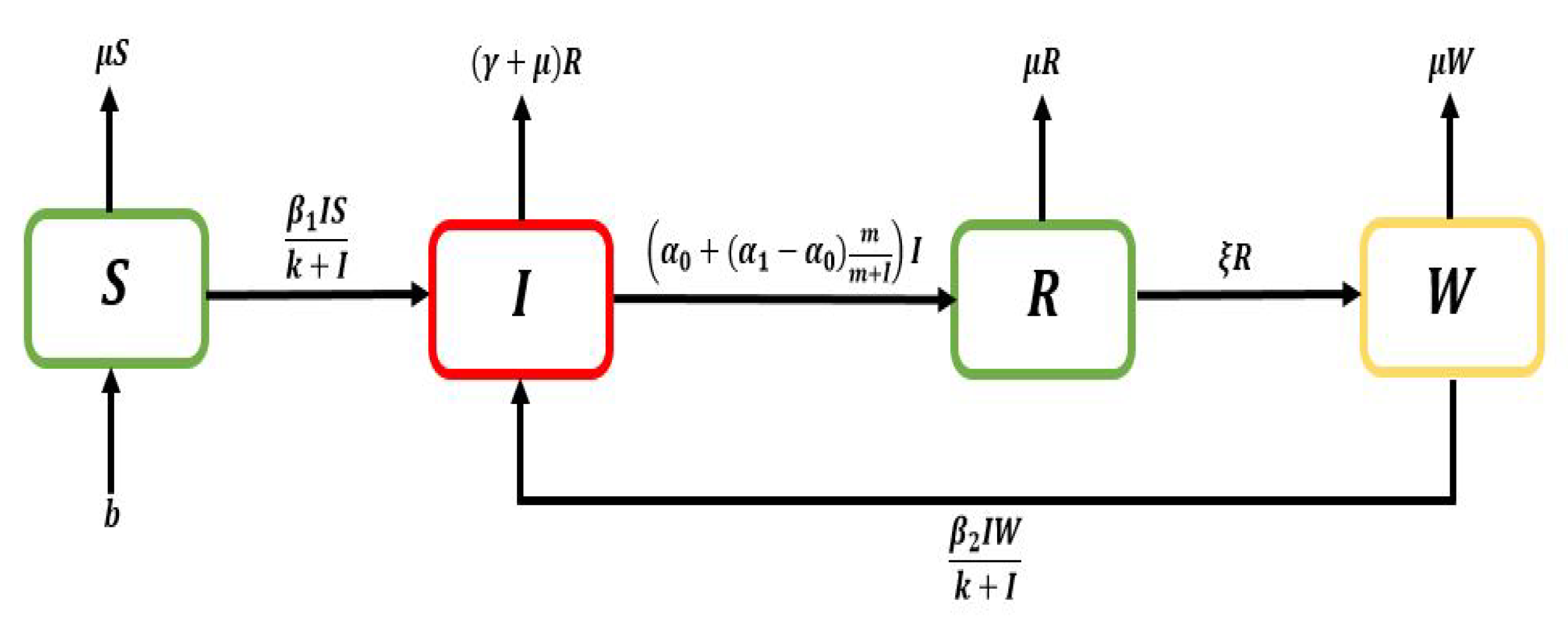
Thoroughly, the population is
, and next, it will be classified into four categories: susceptible
, infectious
, recovered
, and susceptible that previously infected
humans, where
(as shown in
Figure 1). Individuals move from compartment
S to
I as well as
W to
I as with transmission rates:
and
. We have four sub–populations, therefore a nonlinear dynamical system consisting of four nonlinear differential equations established is as follows:
Table 1.
Parameters Description
Table 1.
Parameters Description
| Parameters |
Descriptions |
Units |
| b |
The birth rate |
|
|
The probability of transmission from S to I
|
|
|
The probability of transmission from E to I
|
|
|
The natural death rate |
|
|
The death due to disease |
|
|
The probability rate of waning immune of people |
|
|
The minimum per capita recovery rate |
|
|
The maximum per capita recovery rate |
|
| k |
The intervention levels |
|
| m |
The impact of the number of hospital beds on the ourbreak |
|
3. Mathematical Analysis
3.1. Positivity of Solutions
Lemma 1.
With the non-negative initial values, say and representing the state variables, each of the solutions curves of the model (1) will be non-negative for all . Additionally,
Proof. Let
, so
, and it follows by the first equation of system (
1) that:
It can be re-written as:
Therefore,
Hence,
So,
For the rest of the equations, we can consistently determine the positivity via this method. So, we are able to say that the solution of the model given by (
1) is non-negative for every time
. For the rest of the part of the proof in the considered Theopositivity, we have
, and summing the equations involve in the system (
1), we arrive at the following expression,
□
3.2. Invariant Region
For the biological significance of our model (
1), we will show that the variables and the parameters are non-negative for all time
and analyse the model (
1) in a suitable feasible region
.
Lemma 2.
The feasible region Φ defined by:
with initial condition , , , is positively invariant for system (1).
Proof. Adding the equations of system (
1), we have:
It follows that
, where
denotes the initial values of the total population. Thus
, as
. So, the region:
is a positively invariant set for system (
1). □
3.3. Non-endemic Equilibria and Basic Reproduction Ratio
The non-endemic equilibria of the model (
1) is obtained by setting
, and substituting it into (
1) to obtain:
3.4. The Basic Reproduction Ratio
Here, we have the following matrix of new infection
, and the matrix of transfer
. We can write
The Jacobians of the above matrices at the non-endemic equilibria
respectively are respectively given by
Next, we get the eigenvalues of matrix
are
and
. Moreover, the reproduction ratio is
3.5. The Co-existing Equilibria
System (
1) has a unique co-existing equilibria in the interior of
that is given by
where
Next, we substitution
and
into the second equation in (
1) so yield a cubic equation in
as follow,
where
which for the polynomial (
5) have the roots
or
for
, which can be written by
From (
5), it can be seen that
Hence, we have the following theorem regarding the existence of the co-existing equilibria when
.
3.6. Local Stability of Non-Endemic Equilibria
To investigate the local stability of all equilibria, we linearize (
1), and it yield a Jacobian matrix,
3.7. Local stability of non-endemic equilibria
Theorem 1. The non-endemic equilibria is locally asymptotically stable for and unstable for .
Proof. From Jacobian matrix (
7) at point
, it is yields eigenvalues
. In addition, we get a characteristic equation,
where
Next, choose
. Moreover, if
then the values of
and
are positive. Thus,
is locally asymptotically stable whenever conditions
,
,
, and
is fullfiled. □
3.8. Local stability of co-existing equilibria
Theorem 2. The co-existing equilibria is locally asymptotically stable whenever it exists.
Proof. From Jacobian matrix (
7) at point
, we get a characteristic equation,
where
From (
9), we obtain that
will be negative if
,
,
, and
. If this condition holds, then based on the Routh-Hurwitz criterion, point
is locally asymptotically stable. □
From Theorems 1 and 2, we note that if the value of the basic reproduction ratio is less than one, then the non-endemic equilibria
will be asymptotically stable. Otherwise, the co-existing equilibria
exist and are stable whenever the reproduction ratio is greater than one. Furthermore, we remark that when
the co-existing equilibria
does not exist. In this case,
is a threshold. On the contrary, if
the
becomes unstable and
exist. If the Routh-Hurwitz criterion of equation (
9) holds, then
is asymptotically stable.
Corollary 1. If , , , and then the system (1) undergoes a forward bifurcation at from to .
3.9. Global stability of non-endemic equilibria
Theorem 3. The non-endemic equilibria is globally asymptotically stable for and unstable for .
Proof. Refer to global proving by the various works in [
16,
17,
18,
35], define a Lyapunov function
Differentiating with respect to time yields
Next, from (
1) we get
The value of
if
. Using the relation between the geometric means and arithmetic means, we confirm that
and fulfilled the equality only at
. Thus, the non-endemic equilibria
is globally asymptotically stable if
. □
3.10. Global stability of co-existing equilibria
Theorem 4. The co-existing equilibria is globally asymptotically stable whenever it exists.
Proof. Refer to global proving by the various works in [
16,
17,
18,
35], define a Lyapunov function
Differentiating with respect to time yields
Next, from (
1) we get
where
Next, since a relation between geometric means and arithmetic means is applied, we claim that
. This condition holds only at
. In consequence, a co-existing point
is globally asymptotically stable. □
4. Optimal Control Problem
To control the spread of the disease, we set to suppress the number of transitioned individuals from recovered into susceptible again. Procedures to suppress that transition phenomenon can be conducted through educational efforts, including outpatient; consultancy; or health campaigns. To reduce the number of the
W population with the minimum cost, we constructed the dynamical model in system (1) by adding parameters for the control of educational efforts, namely
. Then, we obtain:
We determine educational effort as an intervention with the objective functions as follows:
where
T is the final time, and
,
is the weight constant and cost of the conducted interventions. The control problem formed from the constraint equation as the equation of each compartment (
10) and the objective function (
11) can form a Hamiltonian equation related to the optimal control problem. Therefore, we use Pontryagin’s maximum principle for the optimal control
satisfying (
10), such that the associated pseudo-Hamiltonian is
where
,
are adjoint variables satisfied i.e.
where the final condition
for
. The necessary and sufficient optimal condition satisfying are obtained, which in turn gives the optimal control
5. Numerical Simulation
This numerical simulation is designed to support the results of the analysis discussed in the previous section. The dynamical population will be compared when some parameter values change. We applied Runge–Kutta Fourth–Order to solve model (
1) using the parameter values in
Table 2 and initial values in
Table 3.
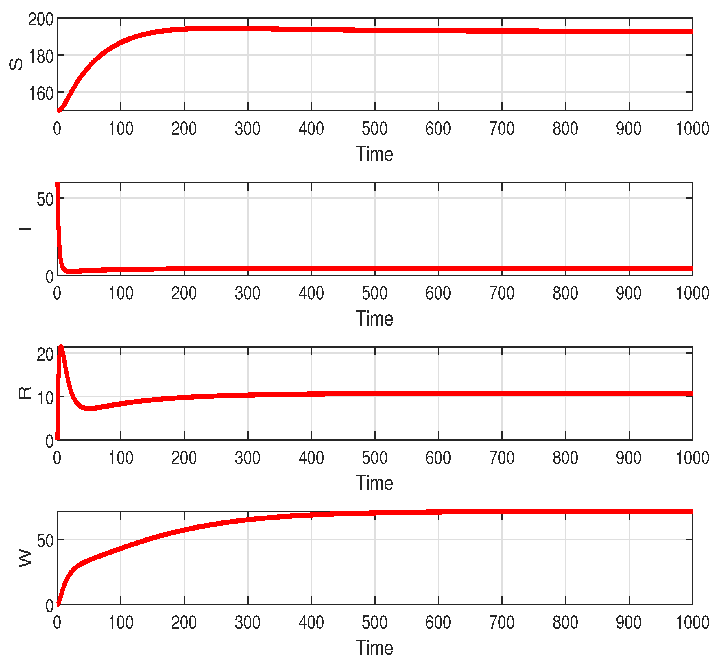
Figure 2 shown that
stable if
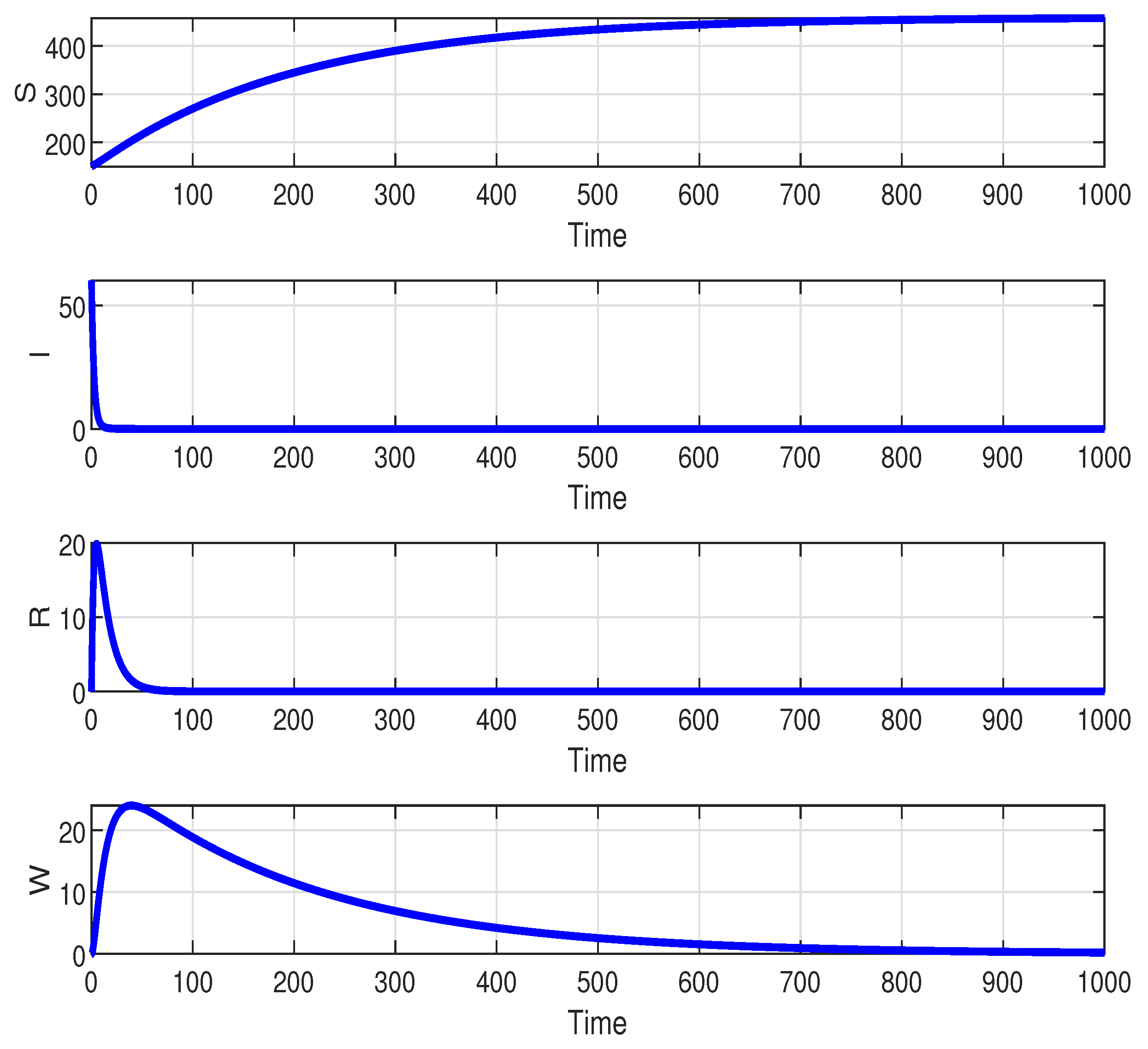
. The population in each compartment converges to a certain amount. This indicates that individuals still exist in the population at a certain time interval. Clearly, it is different if
, which
stable. This case is depicted in
Figure 3. The population in each compartment
I,
R, and
W converge to zero. This situation showed that the disease is free in the system. The behavior of the system (
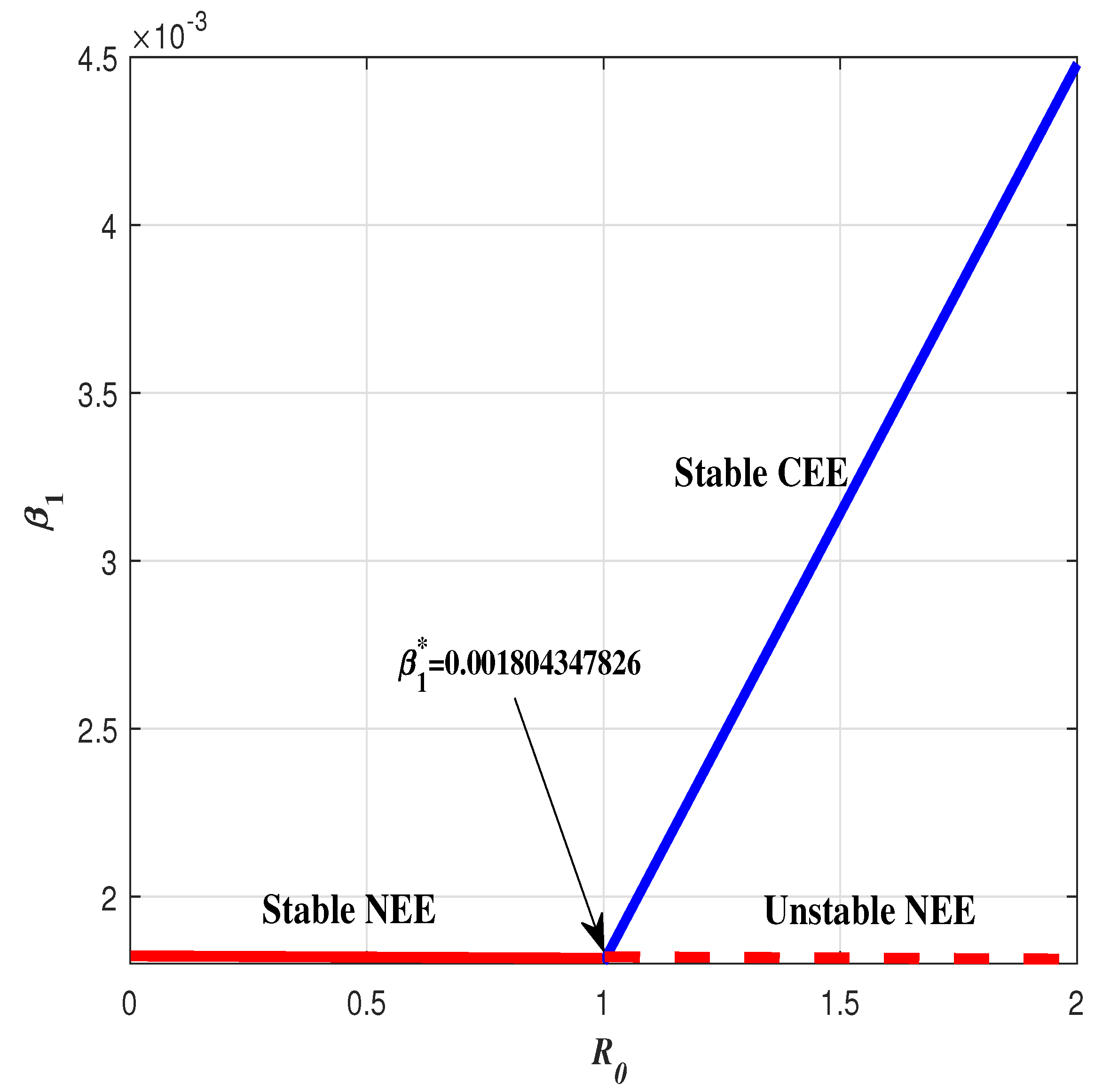
1) related to the changes of parameter
from 0.0018 to 0.01. If
then
stable, meanwhile
unstable precisely when
, where
. This indicates that the system (
1) undergoes a forward bifurcation. This case has been illustrated in the
Figure 4.
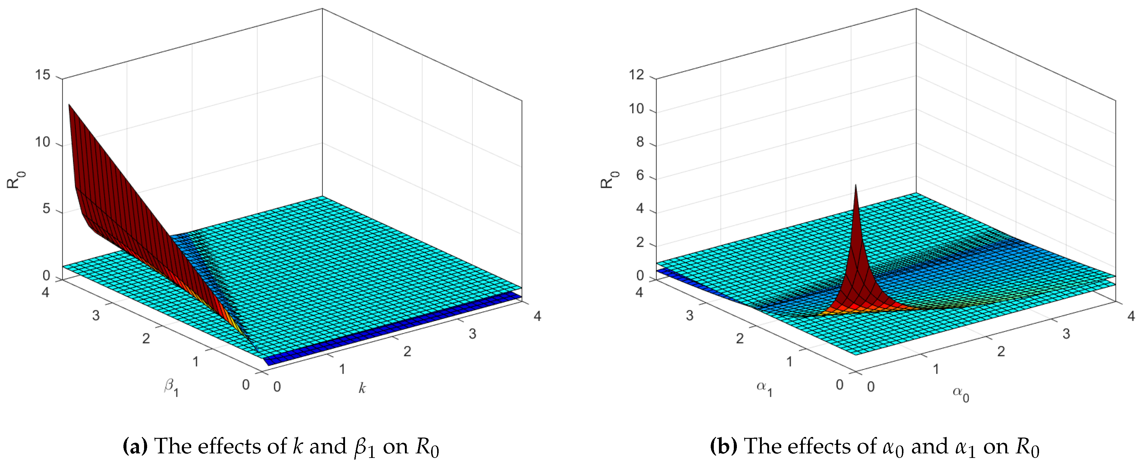
Figure 5a shown that the increase in infection (
) causes
to also enlarge. On the other hand, increased intervention level
k can lead to minimizing
. Thereby, intervention is an important factor in reducing the number of infection cases. Next,
Figure 5b shows that the smaller
and
causes
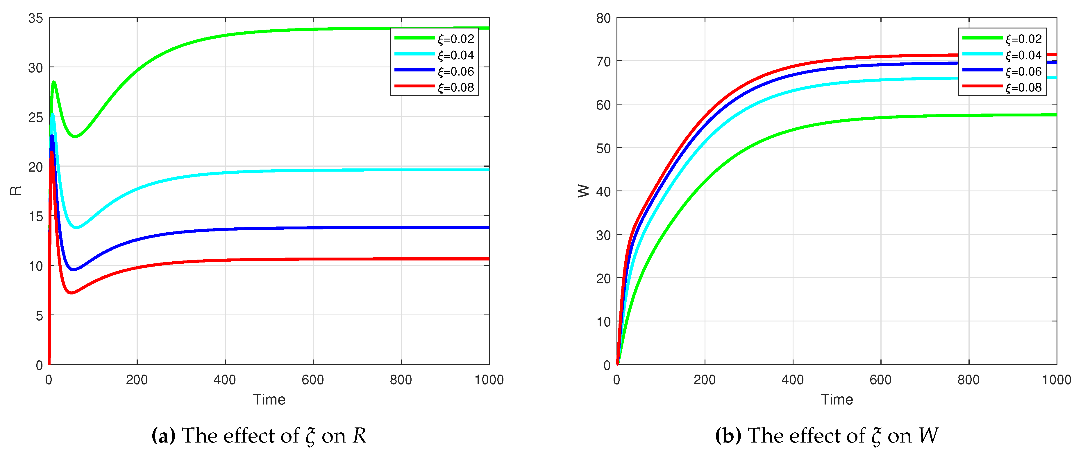
to increase. This illustrates that a lower recovery rate significantly impacts the increase in the number of infections. The condition of waning immunity experienced by individuals who have recovered will certainly affect the dynamics of the system. An increase in the value of
causes the population in
R to decrease. Meanwhile, the population in
W increasing. This behavior is plotted in
Figure 6.
5.1. Numerical Simulation on Optimal Control Problem
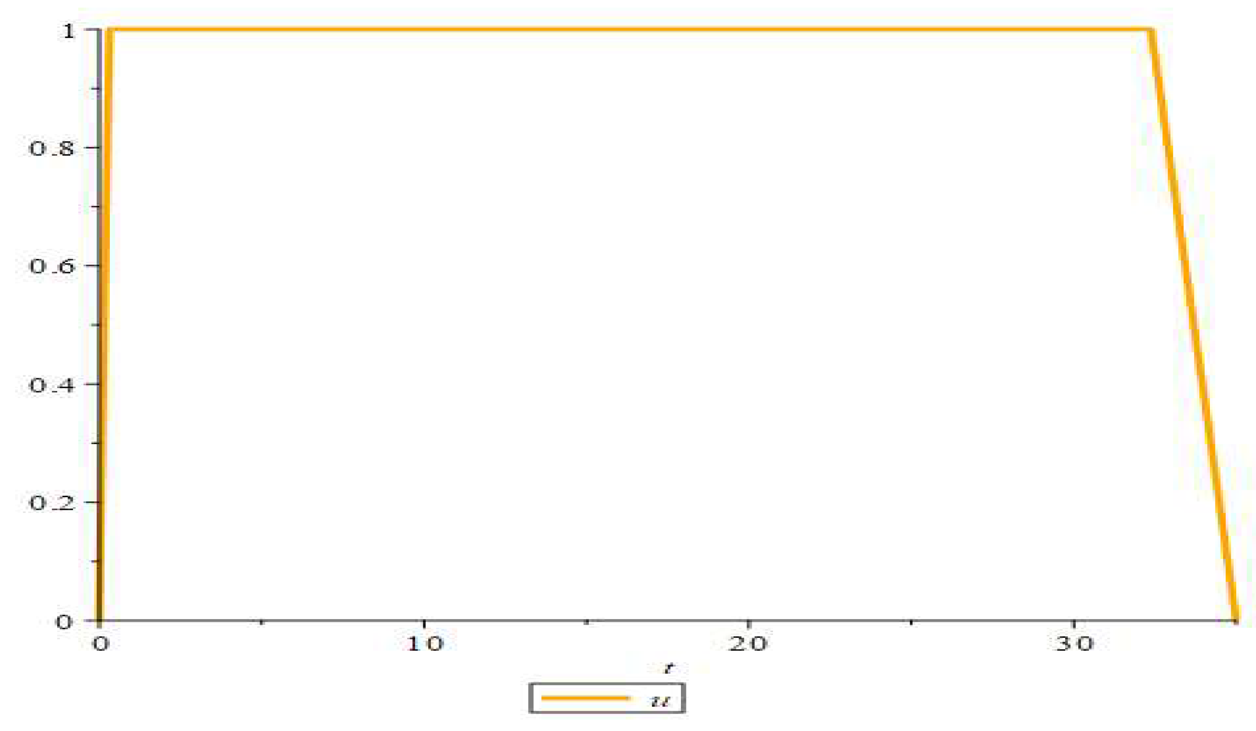
Respective to the objective function on Equation 11, we aim to minimize the number of infected, uneducated injector populations, treatment, and educational efforts. The optimal function graph is shown in the following figure.
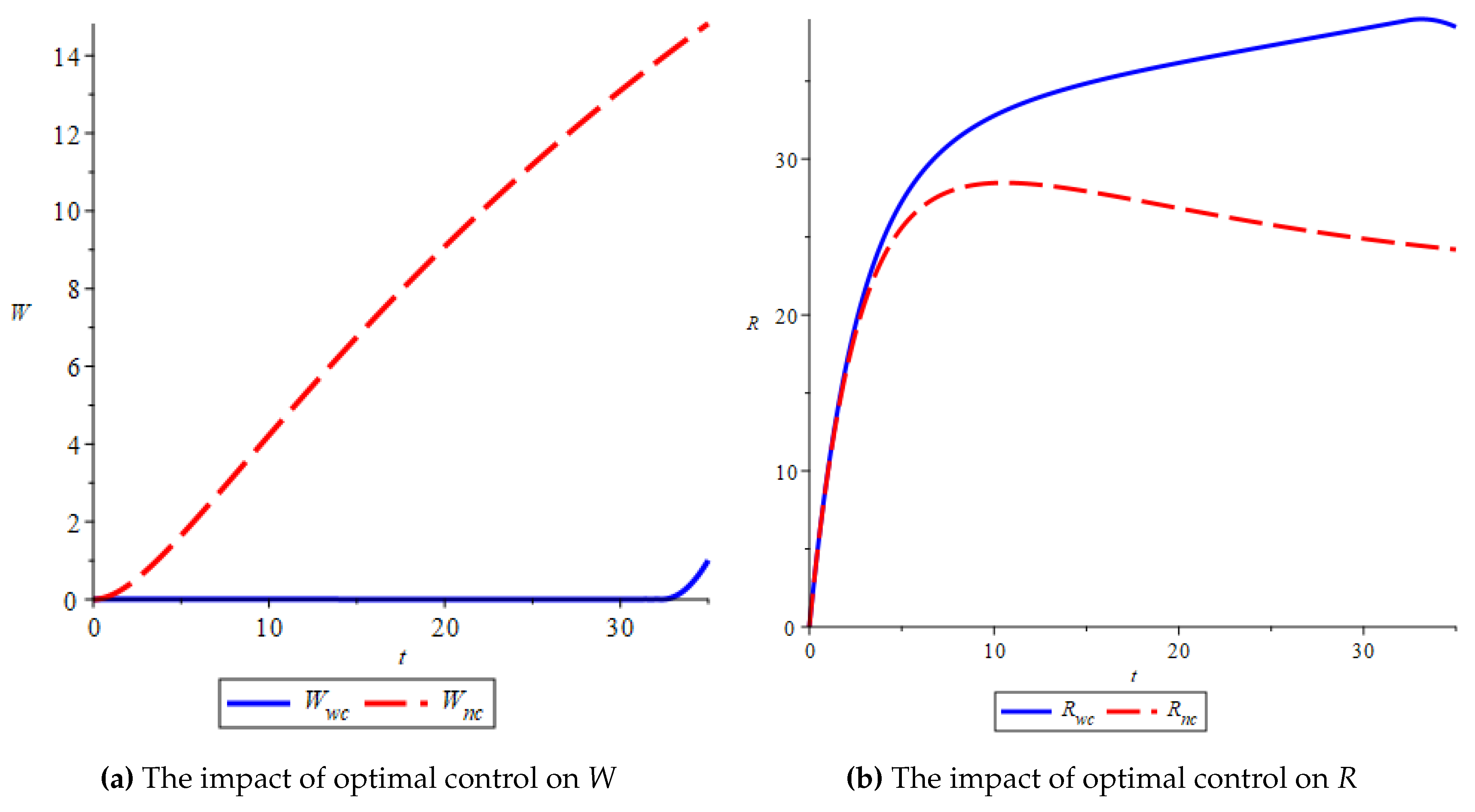
Based on
Figure 8, it is clear that the system with applied optimal control successfully suppresses the number
W population since they were staying on the
R population after healing from infection. The number of
W population stays at the bottom along the control applied, but when at the end, the
W population increase. Referring to
Figure 7, it happens since the control value seems instantaneously to zero. Nevertheless, the optimal control success to reach the aim of the objective function is to minimize the
W population and cost of educational effort.
6. Conclusions
We have formulated a SIRW–type model for an epidemic problem considering waning immunity class with nonlinear incidence and recovery rates. The model is class-based in the form of a differential equations system, where the population is divided into Susceptible , Infectious , Recovered , Susceptible that previously infected . Using a method, namely a next-generation matrix, we obtained the Basic Reproduction Ratio , which is a threshold to control the transmission of disease. Then the simulation results show that the waning immunity factor and half-saturated infection can affect disease transmission. The period of waning immunity and the grade of saturated incidence can spread of disease slowly. The results obtained can be used to reference early prevention of the spread of disease as long as it has similar spreading behavior.
Author Contributions
Conceptualization, N.A. and L.K.B.; methodology, N.A. and L.K.B.; software, N.A., L.K.B., F.I., and S.T.T; validation, N.A. and L.K.B.; formal analysis, N.A. and L.K.B.; investigation, N.A. and L.K.B.; resources, N.A., L.K.B., F.I., and S.T.T; writing—original draft preparation, N.A., L.K.B., F.I., and S.T.T; writing—review and editing, N.A., L.K.B., F.I., and S.T.T; visualization, N.A., L.K.B., F.I., and S.T.T; supervision, N.A.; project administration, N.A., L.K.B., F.I., and S.T.T; funding acquisition, N.A. All authors have read and agreed to the published version of the manuscript.
Funding
This research was funded by Universitas Padjadjaran, Indonesia, via Hibah Riset Data Pustaka dan Daring Universitas Padjadjaran, No. 1549/UN6.3.1/PT.00/2023.
Institutional Review Board Statement
Not applicable.
Informed Consent Statement
Not applicable.
Data Availability Statement
Data sharing not applicable.
Acknowledgments
The authors would like to thank Universitas Padjadjaran to support our project. Also, this project is part of the post doctoral research conducted by LKB.
Conflicts of Interest
The authors declare no conflict of interest.
Appendix A. Proof of the numerical analysis of the non-endemic equilibria
Here, numerically, the Routh-Hurwitz criterion is implemented to assert the Theorem 1 as follows (
):
In addition to
.
Appendix B. Proof of the numerical analysis of the co-existing equilibria
The similar method in the
Appendix A is also used to assert the Theorem 2 as follows (
):
In addition to
.
References
- Alshammari, F.S.; Khan, M.A. Dynamic behaviors of a modified SIR model with nonlinear incidence and recovery rates. Alexandria Engineering Journal 2021, 60, 2997–3005. [Google Scholar] [CrossRef]
- Anggriani, N.; Ndii, M. Z.; Amelia, R.; Suryaningrat, W.; Pratama, M. A. A. A mathematical COVID-19 model considering asymptomatic and symptomatic classes with waning immunity. Alexandria Engineering Journal 2022, 61, 113–124. [Google Scholar] [CrossRef]
- Beay, L. K. Modelling the effects of treatment and quarantine on measles. AIP Conference Proceedings 2018, 1937, 020004. [Google Scholar]
- Rafiq, M.; Ali, J.; Riaz, M.B.; Awrejcewicz, J. Numerical analysis of a bi-modal covid-19 SITR model. Alexandria Engineering Journal 2022, 61, 227–235. [Google Scholar] [CrossRef]
- Gai, C.; Iron, D.; Kolokolnikov, T. Localized outbreaks in an S-I-R model with diffusion. Journal of Mathematical Biology 2020, 80, 1389–1411. [Google Scholar] [CrossRef]
- Singh, H.P.; Bhatia, S.K.; Jain,R.; Bahri, Y. A Study on the Effect of Optimal Control Strategies: An SIR Model with Delayed Logistic Growth, In: Sharma, T.K., Ahn, C.W., Verma, O.P., Panigrahi, B.K. (eds) Soft Computing: Theories and Applications. Advances in Intelligent Systems and Computing, Springer, Singapore, 2021; 1381.
- Elazzouzi, E.; Alaoui, A.L.; Tilioua, M.; Tridane, A. Global stability analysis for a generalized delayed SIR model with vaccination and treatment. Advances in Difference Equations 2019, 532, 1–19. [Google Scholar] [CrossRef] [PubMed]
- d’Onofrio, A.; Manfredi, P. Bifurcation Thresholds in an SIR Model with Information-Dependent Vaccination. Mathematical Modelling of Natural Phenomena 2007, 2(1), 26–43. [Google Scholar] [CrossRef]
- Ebraheem, H.K.; Alkhateeb, N.; Badran, H.; Sultan, E. Delayed Dynamics of SIR Model for COVID-19. Open Journal of Modelling and Simulation 2021, 9, 146–158. [Google Scholar] [CrossRef]
- Rajasekar, S.P.; Quanxin Zhu, M. Higher order stochastically perturbed SIRS epidemic model with relapse and media impact. Open Journal of Modelling and Simulation 2022, 45(2), 843–863. [Google Scholar]
- Cui, Q.; Qui, Z.; Liu, W.; Hu, Z. Complex dynamics of an SIR epidemic model with nonlinear saturate incidence and recovery rate. Entropy 2017, 19(7), 305. [Google Scholar] [CrossRef]
- Li, G-H.; Zhang, Y.X. Dynamic behaviors of a modified SIR model in epidemic diseases using nonlinear incidence and recovery rates. Plos One 2017, 12(4), e0175789. [Google Scholar] [CrossRef] [PubMed]
- Zhang, X.; Liu, X. Backward bifurcation of an epidemic model with saturated treatment function. Journal of mathematical analysis and applications 2008, 348, 433–443. [Google Scholar] [CrossRef]
- Ghosh, J.K.; Ghosh, U.; Biswas, M.H.A.; Sarkar, S. Qualitative Analysis and Optimal Control Strategy of an SIR Model with Saturated Incidence and Treatment. Differential Equations and Dynamical Systems 2023, 31, 53–67. [Google Scholar] [CrossRef]
- Rajasekar, S.P.; Pitchaimani, M.; Zhu, Q. Dynamic threshold probe of stochastic SIR model with saturated incidence rate and saturated treatment function. Physica A 2019, 535, 122300. [Google Scholar] [CrossRef]
- Beay, L.K.; Anggriani, N. Dynamical analysis of a modified epidemic model with saturated incidence rate and incomplete treatment. Axioms 2022, 11(6), 256: 1–21. [Google Scholar] [CrossRef]
- Anggriani, N.; Beay, L.K. Modeling of COVID-19 spread with self-isolation at home and hospitalized classes. Results in Physics 2022, 36, 105378. [Google Scholar] [CrossRef] [PubMed]
- Samui, P.; Mondal, J.; Khajanchi, S. A mathematical model for COVID-19 transmission dynamics with a case study of India. Chaos, Solitons and Fractals 2020, 140, 110173. [Google Scholar] [CrossRef]
- Perry, R.T.; Halsey, N.A. The Clinical Significance of Measles: A Review. The Journal of Infectious Diseases 2004, 189 (Suppl. 1), S4–S16. [Google Scholar]
- Conly, J.M.; Johnston, B.L. Is mumps making a comeback? Canadian Journal of Infectious Disease and Medical Microbiology 2007, 18, 7–9. [Google Scholar] [CrossRef] [PubMed]
- Bankamp, B.; Hickman, C.; Icenogle, J.P.; Rota, P.A. Successes and challenges for preventing measles, mumps and rubella by vaccination. Current Opinion in Virology 2019, 34, 110–116. [Google Scholar] [CrossRef] [PubMed]
- Yang, L.; Grenfell, B.T.; Mina, M.J. Waning immunity and re-emergence of measles and mumps in the vaccine era. Current Opinion in Virology 2020, 40, 48–54. [Google Scholar] [CrossRef] [PubMed]
- Okuwa, K.; Inaba, H.; Kuniya, T. An age-structured epidemic model with boosting and waning of immune status. Mathematical Biosciences and Engineering 2021, 18(5), 5707–5736. [Google Scholar] [CrossRef] [PubMed]
- Zhang, J-Z.; Jin, Z.; Liu, Q-X.; Zhang, Z-Y. Analysis of a delayed SIR model with nonlinear incidence rate. Discrete Dynamics in Nature and Society 2008, 636153. [Google Scholar] [CrossRef]
- McCluskey, C.C. Global stability of an SIR epidemic model with delay and general nonlinear incidence. Mathematical Biosciences and Engineering 2010, 7(4), 837–850. [Google Scholar] [PubMed]
- Enatsu, Y.; Nakata, Y. Stability and bifurcation analysis of epidemic models with saturated incidence rates: An application to a nonmonotone incidence rate. Mathematical Biosciences and Engineering 2014, 11(4), 785–805. [Google Scholar] [CrossRef]
- Chen, Y.; Zhao, W. Dynamical analysis of a stochastic SIRS epidemic model with saturating contact rate. Mathematical Biosciences and Engineering 2020, 17(5), 5925–5943. [Google Scholar] [CrossRef] [PubMed]
- Ammi, M.R.S.; Tahiri, M.; Torres, D.F.M. Global stability of a caputo fractional SIRS model with general incidence rate. Mathematics in Computer Science 2021, 15, 91–105. [Google Scholar] [CrossRef]
- Thirthar, A.A.; Naji, R.K.; Bozkurt, F.; Yousef, A. Modeling and analysis of an SI1I2R epidemic model with nonlinear incidence and general recovery functions of I1. Chaos, Solitons and Fractals 2021, 145, 110746. [Google Scholar] [CrossRef]
- Sun, R. Global stability of the endemic equilibrium of multigroup SIR models with nonlinear incidence. Computers & Mathematics with Applications 2010, 60(8), 2286–2291. [Google Scholar]
- Koufi, A.L.; Adnani, J.; Bennar, A.; Yousfi, N. Analysis of a stochastic SIR model with vaccination and nonlinear incidence rate. Computers & Mathematics with Applications 2019, 9275051. [Google Scholar]
- Zhou, J.; Yang, Y.; Zhang, T. Global stability of a discrete multigroup SIR model with nonlinear incidence rate. Mathematical Methods in the Applied Sciences 2017, 40(14), 5370–5379. [Google Scholar] [CrossRef]
- Jin, Y.; Wang, W.; Xiao, S. An SIRS model with a nonlinear incidence rate. Chaos, Solitons and Fractals 2007, 34(5), 1482–1497. [Google Scholar] [CrossRef]
- Li, T.; Zhang, F.; Liu, H.; Chen, Y. Threshold dynamics of an SIRS model with nonlinear incidence rate and transfer from infectious to susceptible. Applied Mathematics Letters 2017, 70, 52–57. [Google Scholar] [CrossRef]
- Nudee, K.; Chinviriyasit, S.; Chinviriyasit, W. The effect of backward bifurcation in controlling measles transmission by vaccination. Chaos, Solitons and Fractals 2019, 123, 400–412. [Google Scholar] [CrossRef]
- Shan, C.; Shu, H. Bifurcations and complex dynamics of an SIR model with the impact of the number of hospital beds. Journal of Differential Equations 2014, 257, 1662–1688. [Google Scholar] [CrossRef]
- Turkyilmazoglu, M. A restricted epidemic SIR model with elementary solutions. Physica A 2022, 600, 127570. [Google Scholar] [CrossRef]
- Liu, L.; Jiang, D.; Hayat, T. Dynamics of an SIR epidemic model with varying population sizes and regime switching in a two patch setting. Physica A 2021, 574, 125992. [Google Scholar] [CrossRef]
- Arazi, R.; Feigel, A. Discontinuous transitions of social distancing in the SIR model. Physica A 2021, 566, 125632. [Google Scholar] [CrossRef]
- d’Onofrio, A.; Manfredi, P. Behavioral SIR models with incidence-based social-distancing. Chaos, Solitons and Fractals 2022, 159, 112072. [Google Scholar] [CrossRef]
- Giménez-Mujica, U.J.; Anzo-Hernández, A.; Velázquez-Castro, J. Epidemic local final size in a metapopulation network as indicator of geographical priority for control strategies in SIR type diseases. Mathematical Biosciences 2022, 343, 108730. [Google Scholar] [CrossRef]
- Yang, H.; Wang, Y.; Kundu, S.; Song, Z.; Zhang, Z. Dynamics of an SIR epidemic model incorporating time delay and convex incidence rate. Results in Physics 2022, 32, 105025. [Google Scholar] [CrossRef]
- Ndii, M. Z.; Beay, L. K.; Anggriani, N.; Nukul, K. N.; Zhang, Djahi, B.S. Estimating the Time Reproduction Number in Kupang City Indonesia, 2016–2020, and Assessing the Effects of Vaccination and Different Wolbachia Strains on Dengue Transmission Dynamics. Mathematics 2022, 10(12), 2075. [Google Scholar] [CrossRef]
|
Disclaimer/Publisher’s Note: The statements, opinions and data contained in all publications are solely those of the individual author(s) and contributor(s) and not of MDPI and/or the editor(s). MDPI and/or the editor(s) disclaim responsibility for any injury to people or property resulting from any ideas, methods, instructions or products referred to in the content. |
© 2023 by the authors. Licensee MDPI, Basel, Switzerland. This article is an open access article distributed under the terms and conditions of the Creative Commons Attribution (CC BY) license (http://creativecommons.org/licenses/by/4.0/).
