The Epidemiological and Economic Impact of COVID‑19 in Kazakhstan. Agent-Based Modelling

Background. We created agent-based model for short- and longterm forecasting of COVID-19 and for evaluation how the actions of the regulator affected the human and material resources of the healthcare system. Methods. The model was implemented in the AnyLogic software. It includes two state charts – social network and disease transmission. The COVID-19 Essential Supplies Forecasting Tool (COVID-ESFT, version 2.0) was used to determine healthcare resources needed. Results. Satisfactory results were obtained with long-term (up to 50 days) forecasting in the case of a monotonous change in total cases curve. However, if periods of relative stability are accompanied by sudden outbreaks, relatively satisfactory results were obtained with short-term forecasting, up to 10 days. Simulation of various scenarios showed that the most important place for the spread of infection are families. Wherein the maximum number of cases of COVID-19 is observed in the age group of 26-59 years. Due to a set of measures taken by government agencies, the number of cases in Karaganda city was 3.2 times less than was predicted in “no intervention” scenario. Economic effect is estimated at 40 %. Conclusion. Performed model is an attempt to consider as much as possible the peculiarities of the socio-demographic situation in the country. In the future, we will be prepared to some extent for challenges like those we have experienced in the past three years.

Keywords:

Subject: Public Health and Healthcare - Health Policy and Services

1. Introduction

The COVID-19 pandemic has been a colossal test of the strength of the healthcare system around the world, including in Kazakhstan. Unprecedented measures were taken in the Republic to support the industry, which significantly reduced the spread of infection, reduced morbidity, and mortality. The experience of the past months shows that understanding the dynamics by which the disease spreads and making the right decisions is vital in combating and containment of this disease. For more than a hundred years, mathematicians and later epidemiologists have put effort into making models that can predict statistical properties of epidemics. Besides predicting the future state of a pandemic and the number of infections involved, a model to policy makers to take the necessary and optimal decisions is required.

Classical models describe the dynamics of infection spread using systems of differential equations. A significant advantage of models based on the apparatus of differential equations is the possibility of their analytical study. However, SI, SIR, SEIR, SIS and SIRS models fail to effectively model spatial aspects of the spread of an epidemic, the individual contact process, and the effects of individual behaviors, among others [1]. These shortcomings are partially devoid of modern computer simulation models of the spread of the disease. Cellular automata based models are an alternative to using deterministic differential equations, which use a two-dimensional cellular automaton to model location specific characteristics of the susceptible population together with stochastic parameters which captures the probabilistic nature of disease transmission [2,3]. However, the representation of individuals' movement and interactions over the space is no presented. This is an important factor to consider in highly contagious diseases and therefore this methodology gave way to a new approach.

Agent-based models (ABM) are similar to cellular automata-based models but leverage extra tracking of the effect of the social interactions of individual entities. The agent-based model describes a complex system as a collection of many autonomous agents that have their own goals, behavior, and interactions with other agents and the environment. As in the real world, global behavior and trends emerge from the behavior and interactions of individual agents [4,5].

Models of interaction between agents within a system play a vital role in dynamic models of infection transmission [6]. In the past, ABM have been used for tasks such as assessing the spread of smallpox [7], developing strategies for influenza vaccination [8], limiting measles transmission through contact tracing and quarantine [9], assessing the effectiveness of social distancing measures and antiviral prophylaxis against the H5N1 virus influenza A (avian influenza) [10] and the development of evacuation strategies in case of infection by airborne droplets [11].

One of the advantages of agent-based modeling is the ease of modeling various scenarios. For example, the scenario of the universal use of masks in combination with social distancing is simulated in the models of B. Braun et al. [12] and Kai et al. [13]. Based on the experience of applying this approach, the testing policy [14], the strategy for reopening public places [15], the effectiveness of treatment methods [16], and the development of a vaccination strategy were evaluated [12].

Some articles in the literature have used agent-based models to simulate the economic and epidemiologic impacts of COVID-19. For example, a study was conducted on the epidemiological and economic impact of the spread of COVID-19 in the United States. The results show that the trade-offs between economic loss, lives saved, and infections averted are non-linear with social distancing adherence and lockdown duration. The industries that have been hit the hardest are not labour-intensive industries such as the agricultural sector and the construction sector, but those in which jobs are highly valued such as professional services [17].

Inoue and Todo [18] calculated that a possible one-month lockdown in Tokyo would result in a total production loss of 5.3% of Japan's annual gross domestic product (GDP). Dignum et al. [19] proposed a tool to analyze the health, social and economic impacts of a pandemic when the government implements a range of interventions such as closing schools, requiring employees to work from home, and providing subsidies to the public. Silva PCL et al. [20] showed that if it is impossible to introduce a full lockdown, the best solution is the “use of face masks and 50% of social isolation” scenario. This scenario is optimal from the point of view of minimizing the number of deaths, saving business, government, and people revenues.

Zhang T et al. [21] assessed the need for medical resources based on different scenarios involving COVID-19 spreads and interventions. The authors made recommendations on the main investments in health care and the allocation of resources. The extent and nature of changes in health care utilization during the COVID-19 pandemic were highlighted in a systematic review by Moynihan R et al. [22].

Other authors have developed COVID-19 strategies that may be most beneficial in resource-limited settings [23].

One of the goals of modeling is to predict the spread of COVID-19 over time. However, this task faced several problems that did not allow predicting morbidity with a high degree of reliability. Thus, in one of the reviews devoted to the analysis of various models, it is shown that out of 59 predictions in 38% of cases the predicted values were higher than the real ones and in 62% of cases they were lower than the observed values. No differences in accuracy were found between different categories of models, nor within each category [24].

Among the possible reasons is the problem of the validity of the proposed models. In a literature study by Heath et al. [25] it was shown that 65% of the agent-based models presented in the articles did not pass rigorous testing. In another review [26], the author, based on the analysis of 126 agent-based models, showed that most articles (about 87%) do not specify how the presented model or the results were tested. Models are often difficult to test due to unavailability or incompleteness of real data.

Another reason is the high variability in the number of daily cases of COVID-19. Transmission of an infectious disease in a population is a complex phenomenon. His behavior is mainly influenced by interactions between people, and not just by the characteristics of everyone [27]. Interactions can be viewed as social processes [28], such as contacts between people, and as place effects [29]. The complexity of interactions also includes effects over time [30], where outcomes in the past, present, and future affect the decision context; for example, persons already found to be infected are isolated and no longer represent a source of infection. In addition, other factors influence the rate, such as the seasonality of pneumonia, mobility, transmission frequency, use of masks depending on the weather, social behavior, stress, public health measures, etc. During the pandemic, different preventive measures were taken in different countries and the level of compliance with these measures was different, so the dynamics of transmission of COVID-19 had its own local characteristics.

Therefore, determining the transmission rate is an important step in creating a model for the spread of the disease. Some authors rely on the contact probability matrix [31], while others determine the physical proximity of agents using geolocation[13]. Many COVID-19 models have estimated time-varying rates of transmission based on case counts or hospitalization data, or models have inferred changes in transmission rates using estimates of the instantaneous reproduction number of the pathogen [32,33,34].

In this regard, a number of authors consider the stochastic models of the spread of COVID-19. Among them models, which describes a stochastic Markov process [35], and stochastic calculus [36,37], which includes differential equations with stochastic component, such as the Brownian motion (white noise) process [38,39,40]. Scientists developed a stochastic epidemiological model with random fluctuations of parameters [41], with binomial distributions [42]. White noise and jumps were introduced, which corresponded to the different disturbances that can occur [43]. Various scenarios of preventive measures were considered in a stochastic ABM and the influence of the environment on the spread of COVID-19 was analyzed [16,44]. One of the advantages of stochastic model is that it takes into consideration various properties of COVID-19. Among them are the unpredictability of sudden outbreaks of flare disease, long periods of asymptomatic course, sudden declines followed by bursts, as well as unimodal and bimodal progression of daily cases of the disease [45]1.a.i.1.45.

We have created a stochastic agent-based model of the spread of infection in a large city in Kazakhstan. Earlier, the works of Kazakh scientists on modeling COVID-19 were already published in the literature, however, as time has shown, the forecast data had a significant discrepancy with reality.

The main contributions and findings are listed below:

Using the OptQuest optimizer, included in AnyLogic software, to validate a stochastic ABM model for the spread of COVID-19 and use it for short- and long-term forecasting
Determination of age groups and public places of locations most susceptible to the spread of infection in a large settlement of Kazakhstan
Assess how the preventive measures taken by the regulator affect material and human resources compared to six hypothetical scenarios: no intervention, school clause, mask veering, vaccination, combined measures.

2. Materials and Methods

2.1. Study Area

We considered a stochastic agent model of the spread of COVID-19 in a fourth largest settlement of Kazakhstan – Karaganda city. It is a major industrial center of the republic. The city is known as the city with the several hospitals, 7 high schools, and with a population of 500,900 people. In total, 173500 families live in the city.

2.2. ABM Model Implementation

The model was implemented in the AnyLogic University Researcher 8.8.1 software. A demo version of the model on 1:10 scale is available at https://cloud.anylogic.com/model/ba844cef-a41f-4032-8e1f-517e243b8e5f?mode=SETTINGS. It includes two state charts – social network and disease transmission.

2.2.1. Social Network

The entire population was divided into five groups: children attending preschool and school institutions, university students, working adults, non-working adults - each group has its own pattern of behavior (Figure 1). Families are randomly filled with individuals from these categories. The number 1 person, 2 persons, 3 persons, 4 persons and 5 persons families corresponded to the official data of the stat.gov.kz website.

Given the complexity of modeling social contacts, we simplified contacts at both the individual and household levels to model different types of social contacts throughout the day. Social contacts included close contacts over a long period of time with a small number of people, such as family contacts or people who met at school, kindergarten, university, or at work. Brief contact with people in public places, such as shops, hospitals, public transport, was also considered. It was assumed that schools, preschool institutions, shops, and clinics are within walking distance, university students use public transport. Preschoolers, pupils, and university students were in contact within their groups and classes. Working contacts were observed among persons 26-60 years old. According to the classification existing in Kazakhstan, we distinguished between small, medium, and large enterprises. Their number corresponds to the statistics. The filling of enterprises was carried out randomly. We have assumed that for non-working persons, the public places they visit are mainly outpatient clinics, convenience stores and shopping centers where transmission of infection from a carrier to a healthy person can occur. In addition, for other residences, the places of infection are the family, public transport, work, and educational institutions.

2.2.2. Disease Transmission

The spread of infection occurs according to the well-known SEIR model and depends on the number of carrier contacts and the probability of infection.

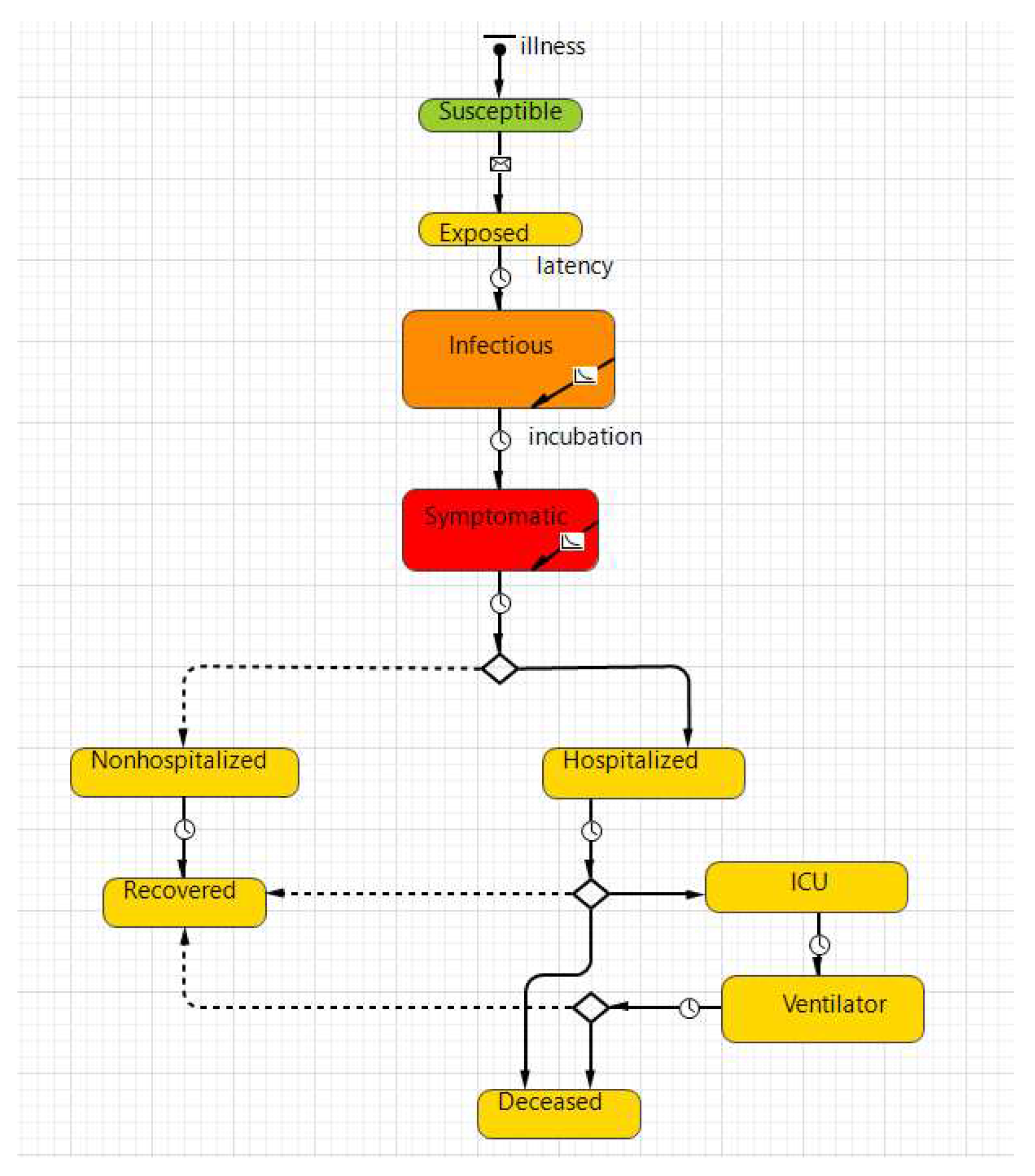
At the start of the pandemic agents are in a “susceptible” state, except for a few initial infections (Figure 2).

Agents are moving or stopping according to their own trajectories. Once susceptible agents meet infectious agents and get infected, the state of susceptible agents is transformed to “exposed.” After a given “latent period,” those individuals become “infectious” which can infect other agents. COVID-19 symptoms appear around incubation period after exposure. Some of the sick, after being diagnosed, remain on outpatient treatment, are isolated at home, and recover soon. The other part is sent to the hospital and, if the condition worsens, they can end up in intensive care and artificial lung ventilation. Outcomes for all patients are recovery or death. Once recovered, the agents can no longer be infectious and cannot be re-infected. This assumption was made, as the risk of reinfection early in the pandemic was low [46].

2.2.3. Model Parameters

Socio-economic and epidemiological parameters of the model are given in the Supplementary Tables 1S, 2S.

The main disease parameter needed to initialize the model is the transmission rate (β). The parameter β can be physically understood as follows: let in a homogeneously mixed population a randomly chosen susceptible person has c contacts per unit time with other persons, and let p is the probability of disease transmission from an infected person to a susceptible, then, the quantity β is defined by the relation: β=-c ln(1-p) [47]. For sufficiently small p, β = cp. Thus, β is the product of contact rate and disease transmission probability.

Epidemic rate depends on a large number of factors. Mitigation measures are mainly aimed at keeping the number of contacts between contagious and susceptible people, as well as the probability of infection by contact, as low as possible. Among the factors affecting the incidence, one can indicate such as migration, quarantines, lockdowns, heterogeneous mixing of the population, insufficient testing, the presence of asymptomatic cases, the simultaneous presence of several strains, etc. It is very difficult to assess which part of the population and how strictly adheres to restrictive measures in their daily lives. All this leads to the fact that in reality the dynamics of the spread of infection is different from the classical epidemiological process. Transmission rate and contact rate are functions of time and have a stochastic character (the Figure 3 shows a fragment of the daily number of cases of COVID-19 in Karaganda).

Therefore, many authors set the contact rate using the function of probability distribution. In various studies, normal distribution [48], lognormal [49], Bernoulli distribution [50], Geometric distribution [51], binomial distribution [52] were used in modeling. We defined probability of contacts as

p (c = x) = G e o m e t r i c (x, \frac{1}{1 + c})

were average daily contacts c= 6 [53].

To evaluate parameter p-disease transmission probability, we used the OptQuest optimizer, included in AnyLogic software. The difference between the modelled and actual total cases of COVID-19 was chosen as the target function. The optimization consisted in minimizing the target function. As a result, in different pandemic time periods different values p were obtained.

One more parameter is incubation period. In the literature, data on the incubation period vary widely: from 1 to 14 days [54,55]; the average value was 5.8 days (95% CI from 5.0 to 6.7) [56]. According review, that included 53 articles, the pooled mean incubation period of COVID-19 was 6.0 days (95% CI 5.6–6.5) globally [57]. We set an incubation period of 6 days.

2.3. Data Collection

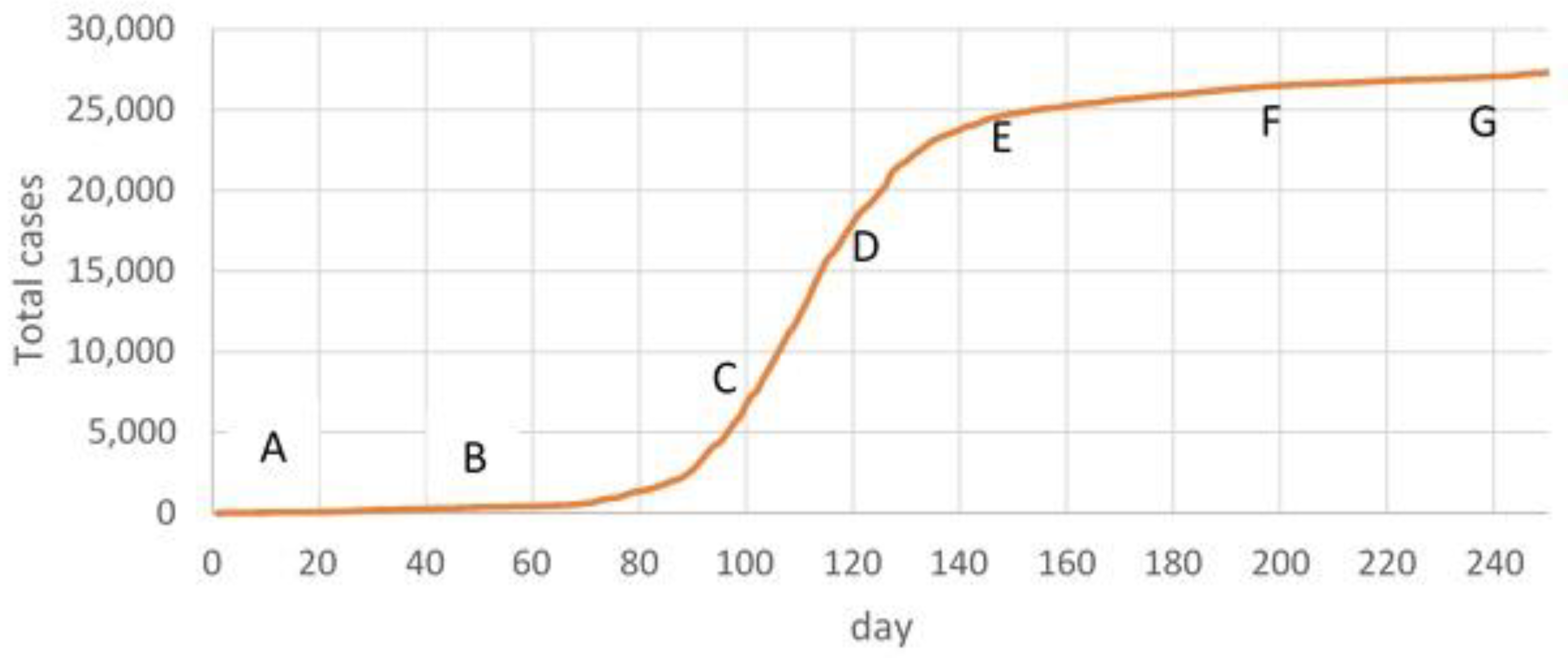
We analyzed total cases of COVID-19 between 10 March 2020 and 16 November 2020 (250 days). Data were collected from the information system of the Ministry of Health of the Republic of Kazakhstan (Figure 4).

We chose this time interval because the total cases curve includes intervals of relatively constant growth and inflection points in which the slew rate changes.

First time frame (AB) includes 50 days from 10 March 2020 to 30 April 2020. Next time frame (BC) was 50 days, from 01 May to 19 June. The third time frame (CD) was 20 days, from 20 June to 09 July. DE - 30 days from 10 July to 08 August, EF – 50 days from 09 August to 27 September and FG – 50 days from 28 September to 16 November 2020.

For each of this time frames:

using the Optimization mode of AnyLogic, the optimal value of p-disease transmission probability was selected

to see the effect of the stochastic variation of the contact rate, Monte Carlo simulation methods were carried out, with each run of the model containing 50 iterations. In each iteration, a different value from within the defined range for the contact rate was used. This produced output values that are value ranges rather than point estimates. Next, the mean values for each run were found

to validate an agent-based model in each time frame we compared the output of the model to real data

based on each of these time periods, total cases were predicted for the next 50 days

we used the mean absolute percentage error (MAPE) metric for contrasting between simulated and true values. MAPE was chosen because of its scale independence property, which would remove bias due to the size of the test data from the models. It is calculated by normalizing the average error at each point.

M A P E = \frac{1}{n} \sum_{t = 1}^{n} |\frac{A_{t} - F_{t}}{A_{t}}|

where At is the actual data, Ft is the simulated data at time t and n is the number of days.

Model accuracy was evaluated as highly accurate (MAPE%<10), good (MAPE%: 10-20), reasonable (MAPE%: 20-50), and inaccurate forecasting (MAPE%>50) [58].

2.4. Scenario Setting

Base Scenario (BS) – No Intervention

Base Scenario simulated a completely natural epidemic transmission process without any intervention measures. For that we estimated parameter p according to the basic reproduction number R0, which is defined as the average number of secondary cases produced by a typical primary case during its infectious period in a completely susceptible population [59]. Parameter p can be inferred based on a mathematical expression as R0 = cpDi, where Di is the average infectious period [60]. Therefore, parameter p is inferred as:

p = R0 / cDi

We set R0 =3, Di=6 days (we have established that the patient is contagious during the incubation period before the onset of symptoms, after which he is immediately isolated) [61].

Scenario 2 – School Closure (SC).

This scenario includes the closure of schools, preschools, and universities. The aim is to reduce social contacts, to cut transmission chains in the community.

Scenario 3 – Mask Wearing (MW)

In practice, 100% mask wearing is not achievable. Tian et al. [62] developed a simple transmission model that incorporated mask wearing and mask efficacy as a factor in the model. For wearing masks, they found that wearing masks reduces R0 by a factor (1-mp)2, where m is the efficacy of trapping viral particles inside the mask, and p is the percentage of the population that wears masks. In practice, 100% mask wearing is not achievable. We considered scenario with 50% mask usage and 50% mask efficacy [63], then (1-mp)2=0.56

Scenario 4 – Vaccination (VS).

In this scenario, we assumed that the population was vaccinated at an average rate of 0.003% of the population, which corresponded to the actual vaccination rate in Kazakhstan [64].

Scenario 5 – Combined Measures (CM)

This scenario includes mask wearing, school closure and the population vaccination.

Scenario 6 – Real Situation Simulation (RS)

For each scenario, the following outcomes were obtained:

the number of infected people at home, in educational institutions, at work, in transport, in stores
the number of infected people among different age groups of the population
number of doctors, auxiliary medical and technical personnel needed
number of beds required for hospitalized persons
the cost of devices, medicines, chemicals and other materials

The COVID-19 Essential Supplies Forecasting Tool (COVID-ESFT, version 2.0) was used to generate a forecast model of the healthcare resources needed [65].

3. Results

3.1. Model Validation

During the fitting step, in Optimize mode, we specified the fixed seed value. In this case random number generator is initialized with the same value for each model run, and the model runs are reproducible. The found optimal values of p-disease transmission probability for each time interval are presented in the Table 1.

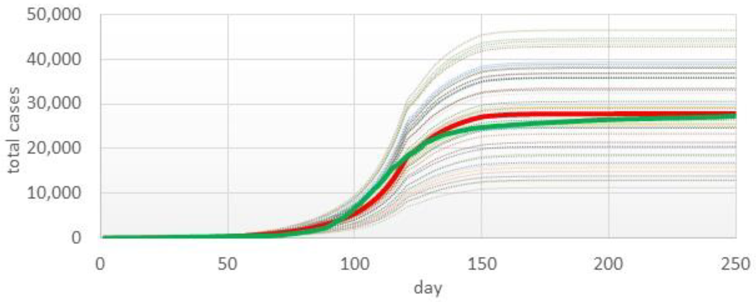
Then we created a Monte Carlo experiment with 50 iterations. Random seed (unique simulation runs) was selected. In this case random number generator is initialized with the same value for each model run, and the model runs are unique (non-reproducible). The fitting results in the form of an average value over all iterations and real data are shown in the Figure 5.

At the initial moment of modeling, the largest error between the model and real data was observed in the AB time frame. This difference can be explained by several reasons. The first is mathematical. At the beginning of the COVID-19 pandemic, with a small number of cases, small differences gave a large error rate. Another reason is the possible overdiagnosis in the early days of the spread of the disease, when diagnostic tests had not yet been developed and the diagnosis was made according to the clinical picture, and increased alertness was observed among doctors. The third reason may be inaccuracy in the duration of the incubation period since there are various data on this parameter in the literature [56]. In other time frames good and high accuracy were obtained. In general, the accuracy of the model was 72%.

3.2. Prediction Simulation

Some time frames in the Figure 4 were chosen as a training, and on its basis, while keeping all parameters unchanged, a forecast was made for 50 days.

3.2.1. Forecasting Based on Time Frame AB

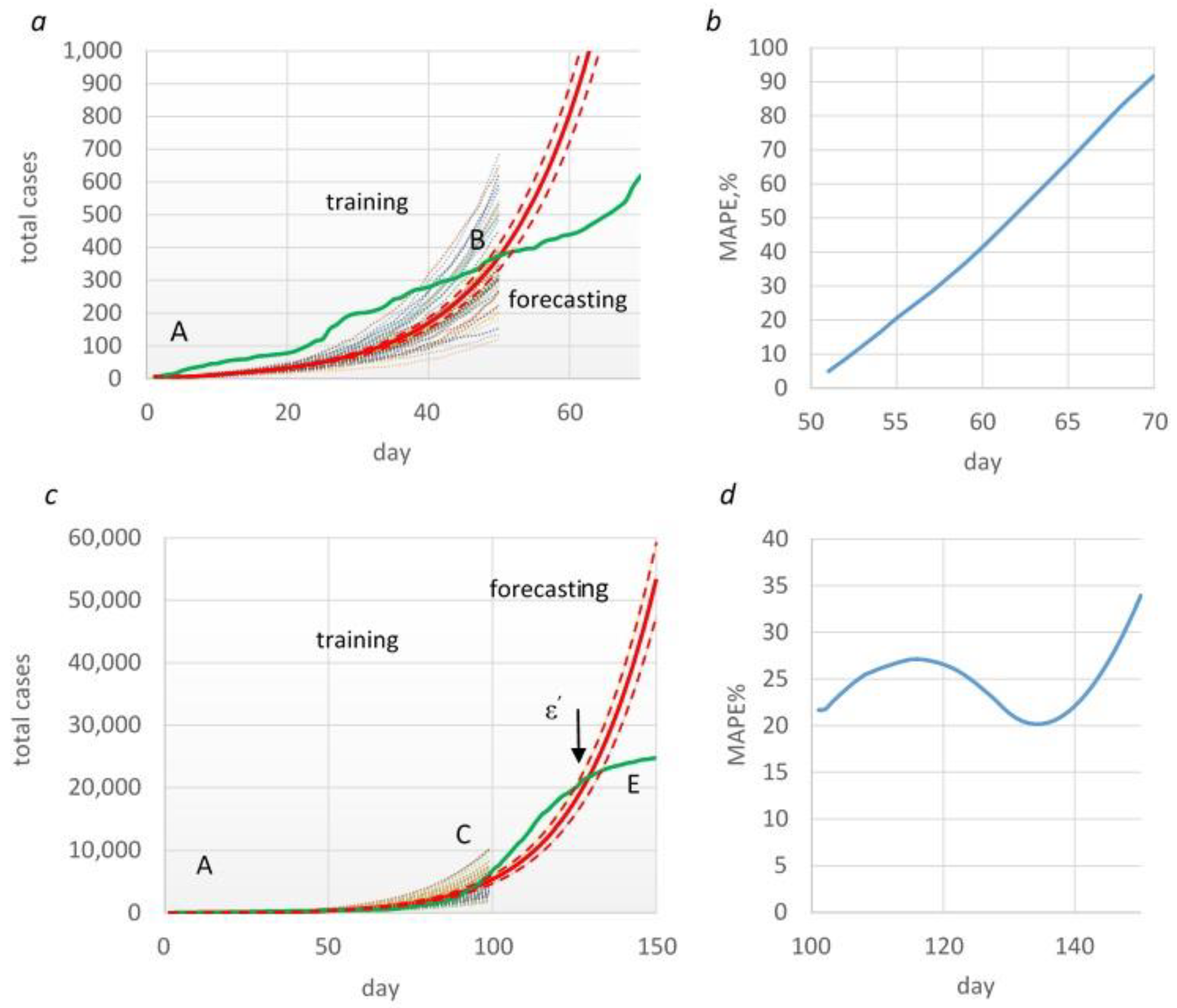
Based on the first training time frame (from days 1 to 50), total cases were predicted using the Monte Carlo procedure (red line, Figure 6a). The predicted data were compared with the actual data (green line). Forecasting accuracy (MAPE) for each of these days is shown in Figure 6b.

To uncover how the MAPE (%) changes with an increase in the duration of the forecast, we presented the results of forecasting for every 5 days in the Table 2.

As already noted in this section, at the fitting stage, a large difference was obtained between real and model data. This was also reflected in the results of forecasting. In this test time frame, the growth of total cases in the model is exponential, while in real data there is a linear trend (Figure 6a). Accordingly, the prediction accuracy also decreased over time. So, if on the 5th and 10th days there were good and reasonable forecasting, then on the 15th day – inaccurate.

3.2.2. Forecasting Based on Time Frame AC

In this case, the AC segment was used as the training time frame, and the prediction was carried out on the CE segment. Approximately on the 126th day from the beginning of the observation, an inflection point (ε’) is observed on the curve, when the rate of growth of total cases slows down (Figure 6c).

From this point on, the forecasting curve and real curve have different dynamics. In this case, according to MAPE, forecasting with an acceptable accuracy of <50% is possible over the entire 50-day segment (Figure 6d). However, in the last 10 days, the relative prediction error (APE%) ranged from 52 to 116%.

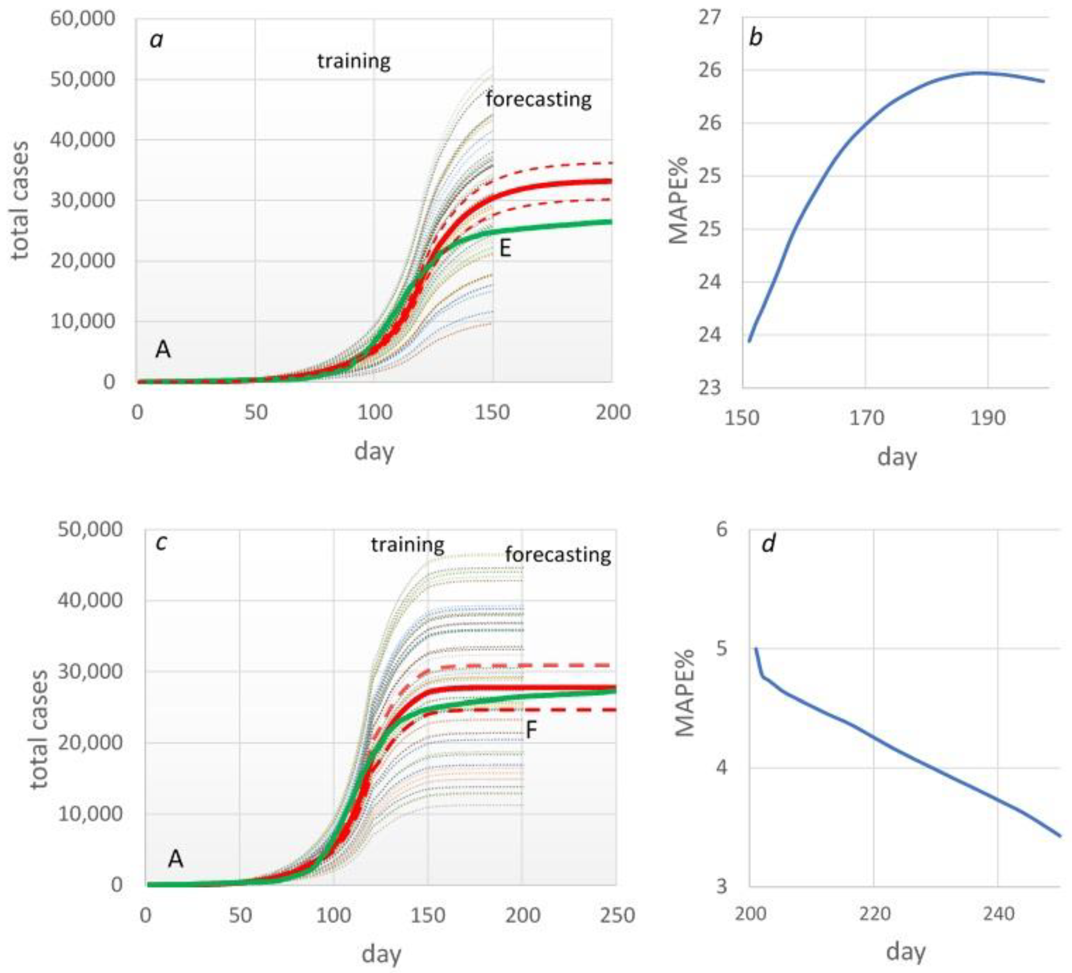
In time frames EF and FG, the total cases curve is relatively linear. Therefore, the prediction accuracy, based on training time frames AE and AF, were higher than in previous cases. So, when forecasting from 151 to 200 days, MAPE varied within 24-26%, which can be considered as a “good” level of prediction (Figure 7a, b). And in the period from 201 to 250 days, the accuracy was 95-97%, i.e. high level (Figure 7c, d).

3.3. Epidemiological Impact of COVID-19

In this section, we have considered various hypothetical scenarios for the spread of the disease. Our goal is to identify public places where there is an intense transmission of the infection, as well as to identify the social groups of the population most susceptible to infection. We wanted to assess how effective the protective measures taken by local and central executive bodies were in terms of public health and in terms of resource costs.

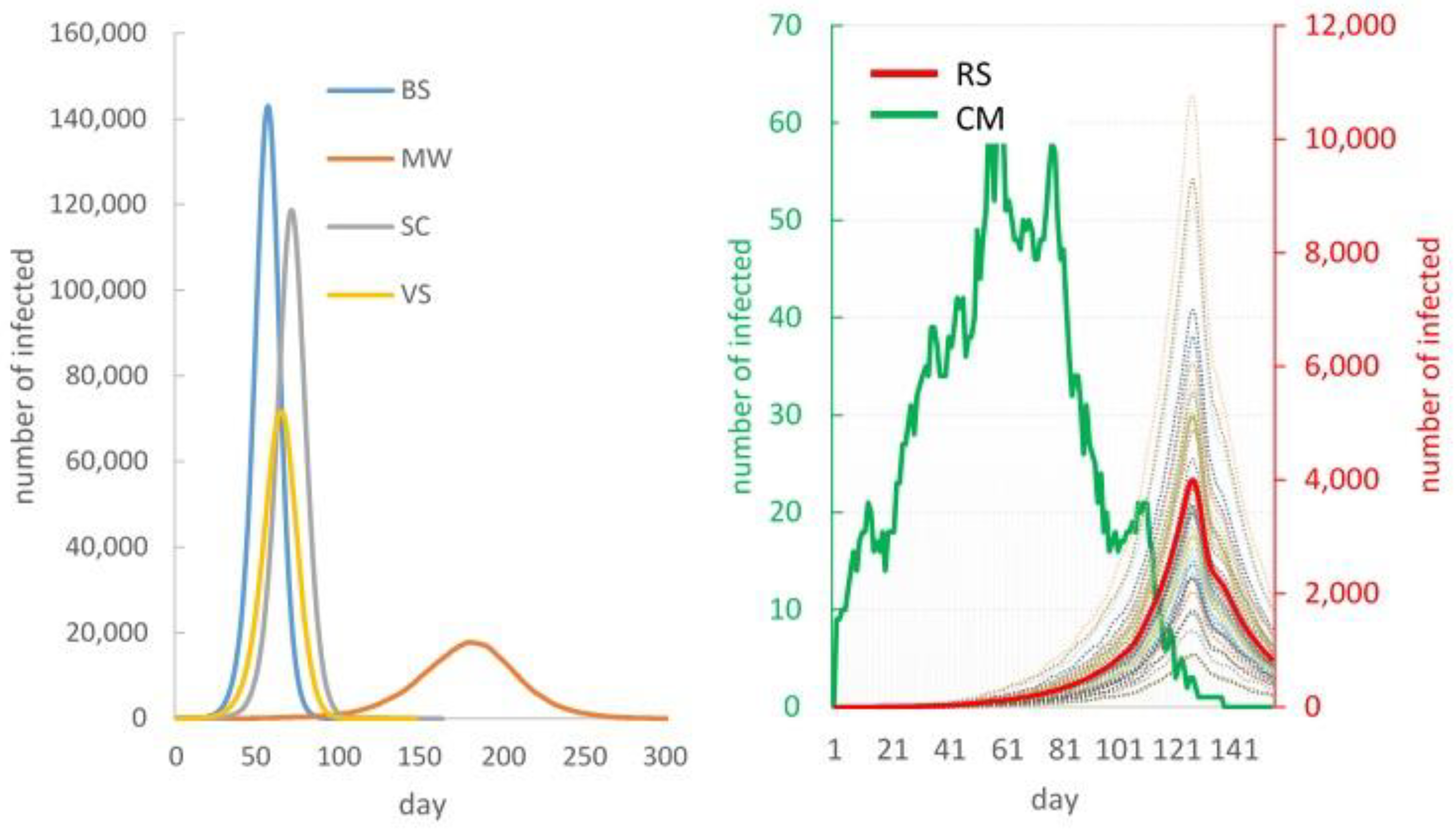
In the absence of any control measures (Base scenario), it is expected that the peak of infection will occur around day 58 of the pandemic and the number of infected on that day will be about 140,000 thousand or 28% of the population (Figure 8), and then their number will decline and reach zero on day 130. We predict that by this point in time 471,746 (94%) of the city's residents will have been ill.

Interventions were able to slow or stop the spread of COVID-19. According to the SC scenario, the peak incidence will be reached somewhat later - on day 72, and in general, the pandemic will last 145 days. Vaccinating reduced and delayed the peak infection to 71,273 cases on day 66, mask wearing – to 17,701 on day 182. According to scenario SC, total cases will decrease by 7% compared to the baseline scenario, according to scenario MV - by 54%, according to scenario VS - by 35%. The combination of all these methods (CM scenario) gives an effect of 99%. In the reality, the total cases amounted to 145,044, which corresponds to a 70% decrease compared to the base scenario (Supplementary Table 3S).

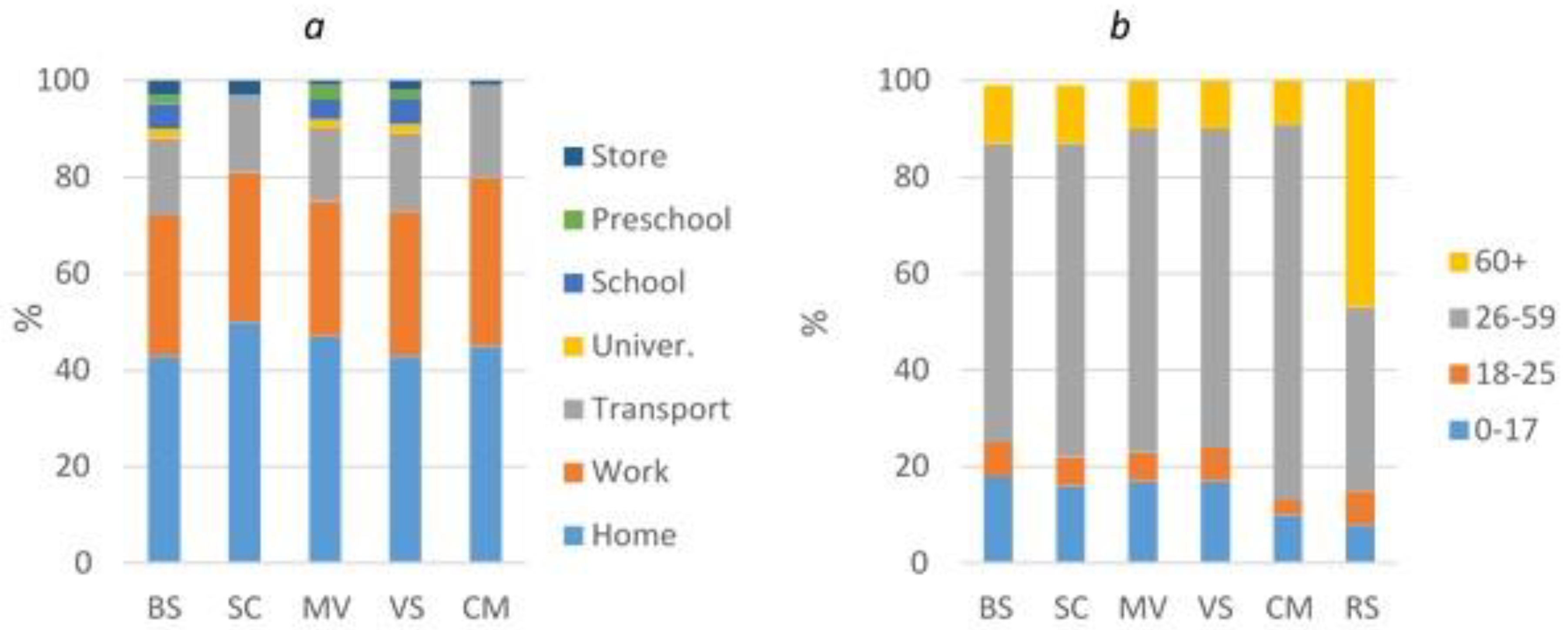
Computer simulation showed that in the Base scenario, the largest number of infections occur at home (43%), then at work (29%), in transport (16%), in education institutions (9%) and stores (3%, we remind you that in our model, stores are within walking distance of the house and are frequented by older people). For other scenarios, a similar ratio is observed (Figure 9a, Supplementary Table 3S).

With reference to published data, it is known that among those infected with COVID-19, the most severe outcomes were in elderly patients, including the highest mortality rates, while younger infected individuals, especially children aged 1 to 18 years, if not present at all. symptoms are much more likely to be mild [66,67]. This, however, does not mean that older people necessarily play a leading role in the spread of COVID-19 in society. Understanding the role of age in transmission and disease severity is critical for determining the likely impact of social-distancing interventions on infection transmission, and for estimating the expected global disease burden.

According to the results of modeling BS, SC, MV, VS, the maximum number of cases of COVID-19 is observed in the age group of 26-59 years, i.e. among working people (Figure 9 B, Supplementary Table 4S). The proportion of this age group ranges from 62% to 78%. Then model suggested that 10-18% of all infections occurred in those aged 0-17 years. The minimum number of cases is among young people 18-25 years old (3-7%) and among elderly people over ≥60 years old (9-12%). Model could not reproduce the observed age distribution of cases - number of cases in children was overestimated and cases in older adults were underestimated. In the reality, the proportion of older people was 47% and the proportion of children was 8%.

3.4. Economic Impact of COVID-19

In this section, we assessed the cost-effectiveness of the preventive measures taken by public health authorities. To do this, we compared the real costs of human and material resources with the costs under other hypothetical scenarios. The COVID-19 Essential Supplies Forecasting Tool (COVID-ESFT, version 2.0) [65] was used to generate a forecast model of the healthcare resources needed.

As the Table 3 shows, the best way to reduce the burden of COVID-19 is to combine all the protections listed above. Theoretically, in such a scenario, we would observe only 159 hospitalized persons. The real situation was not so optimistic, but the results of the simulation showed that the maximum compliance with the requirements of the regulatory authorities contributed to a significant improvement in the epidemiological situation compared to the baseline scenario. Thus, closing schools reduces the number of hospitalized by 7%, the mask wearing mode - by 54%, vaccination - by 35%. In the reality, the number of hospitalized people was 37,287, which is 70% less than in the baseline scenario.

A similar effect is observed in intensive care units and in artificial ventilation units.

3.4.1. Healthcare Human Resource (Medical Practitioners, including Physicians, Nursing Professionals, and Paramedical Practitioners)

One of the critical issues during the pandemic has been the staffing of the COVID-19 response. According to our simulation, the implementation of various preventive measures does not lead to a decrease in the total number of workers involved in the fight against the disease. Under all scenarios, 1970 medical workers are required in hospitals. An exception is the ideal scenario of strict compliance by all people with a whole set of measures. As for other categories of workers, according to the Mask wearing scenario, a decrease in the need for cleaners is predicted by 19%, while in the reality this decrease was 46% (Table 4).

Similarly, measures taken have significantly reduced the need for ambulance personnel. If in the base scenario the demand for 4,458 workers was predicted, then in the mask wearing mode – 3,611, in the real situation the demand was 2,412 workers. Calculations show that the need for technical staff was also in reality significantly lower than in the first four scenarios.

3.4.2. Hospital Beds

The total bed capacity of the city's hospitals is 7,430 beds, of which 4,256 are for seriously ill patients and 202 for patients in critical conditions. During the pandemic, it became necessary to increase the number of beds (Supplementary Table 5S) and for this purpose, infectious diseases departments in all hospitals were expanded and additional wards were opened. According to our data, the greatest need for additional beds occurs in intensive care units and in artificial ventilation units.

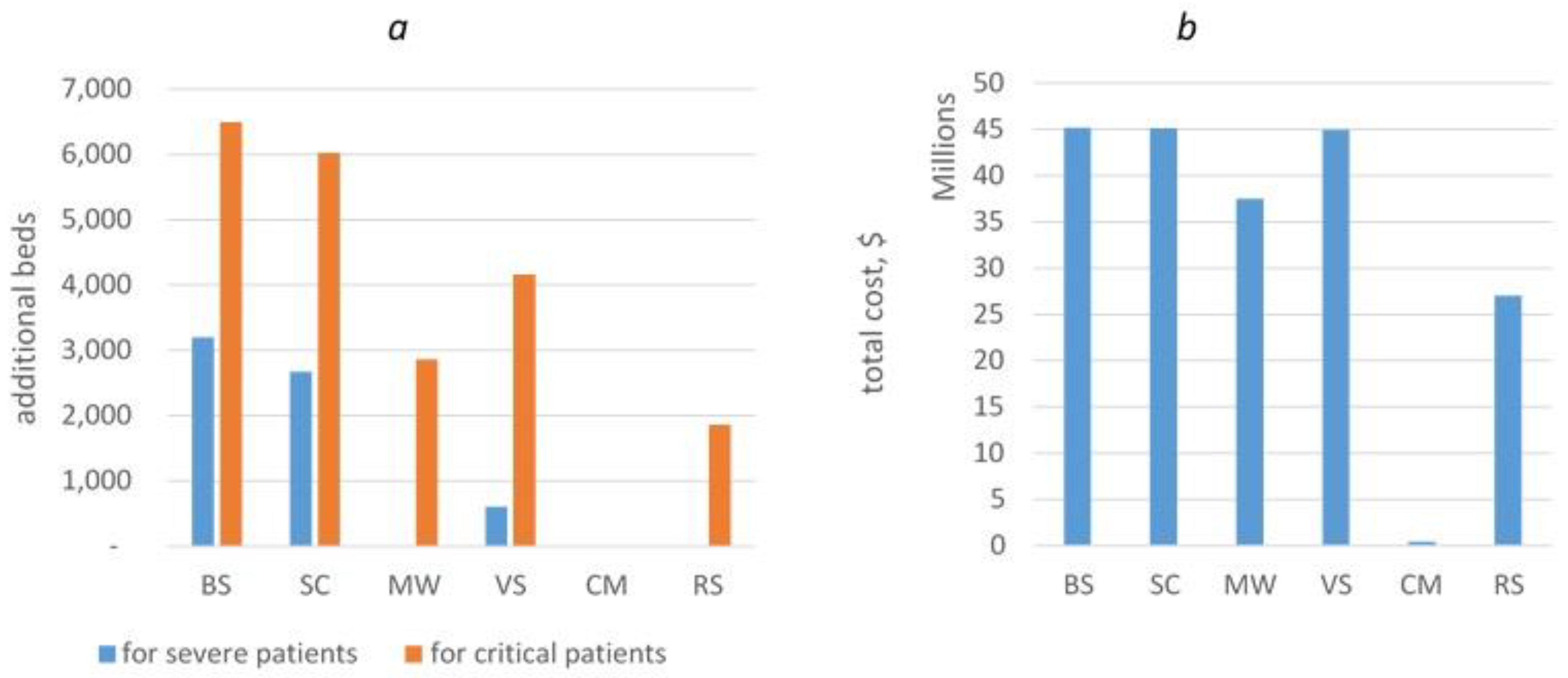
According to the results of the simulation of the basic scenario (Figure 10a), a shortage of 3,198 beds (75% of available) for severe patients and 6496 for critical cases is predicted, which requires a 32-times increase in their number. Intervention measures make it possible to alleviate the situation with the bed fund. According to the VS, the need for additional beds is 601 for severe ill patients and 4,162 for critical cases, in the MW there will be a shortage of beds only for critical cases – 2,861. For the current number of patients, the deficit is 1,857 beds for critical patients, which is 9.2 times more existing fund.

3.4.3. Equipment, Pharmaceuticals, Consumables, and Accessories

The Supplementary Table 6S performs the costs of goods, according to the price list on the site [65]. Base scenario costs are projected at $45,174,975. School closure and vaccination scenarios do not reduce the cost of equipment and supplies. But in Mask wearing mode, costs are reduced by 17% to $37,487,881, while in the reality they are $27,008,080, which saves 40% of costs compared to the base scenario (Figure 10b).

4. Discussion

4.1. The Findings and Their Implications

On May 28, 2023, all coronavirus restrictive measures were lifted in Kazakhstan. It is difficult today to assess the economic and social damage caused by the pandemic. Kazakhstan, like many other states, did not yet have experience in dealing with such rapidly spreading infections, with severe complications and high mortality. The pandemic proceeded differently depending on the geographic, economic, and demographic situation of countries. Many other factors, about which there are already enough publications in the scientific literature, also had an influence. In Kazakhstan, from the first days of the appearance of patients, strict restrictive measures were taken, which made it possible to pass this period with relatively small losses. Today it is time to reflect on the experience of the previous three years of fighting the pandemic, evaluate the effectiveness of the strategy used, and prepare a scientific basis for predicting the epidemiological situation in the event of similar situations in the future. Modeling is the best tool for this. We have created a stochastic agent model of the spread of infection, as the most realistic reflection of the daily activity of various segments of the population in the face of many uncertainties. Such uncertainties include adherence to restrictive measures, susceptibility to infection, susceptibility to a vaccine, the duration of the disease, the influence of environmental factors, etc.

One of the tasks that we set ourselves is the task of forecasting based on the created model. Total cases were used as a predictor to predict the spread of COVID-19. Satisfactory results were obtained with long-term (up to 50 days) forecasting in the case of a monotonous change in this indicator. However, the development of events has shown that the dynamics of daily incidence is oscillatory, and periods of relative stability are accompanied by sudden outbreaks, the nature of which has not yet been explained. As a result, inflection points appear on the Total cases curve. On Figure 4 at least two such points can be identified. In this case, relatively satisfactory results were obtained with short-term forecasting, up to 10 days.

The spread of the infection largely depends on the behavior of various social groups, on their adherence to precautionary measures, on age, health, mentality, marital status, and other factors. Thus, it is known that the most socially active are young people, among them there are more contacts. In some countries, there are many lonely old people, they are more susceptible to severe forms of the disease and their treatment takes longer. Knowledge of such features allows you to prepare in advance for various scenarios. The city of Karaganda has more than 173 thousand households. 35% of families consist of 4 or more people. We noticed that there is a very high risk of domestic infection - up to 50% of infections occur at home. The use of various preventive measures in such cases did not give any improvement. Although wearing a mask is effective in blocking close-contact transmission, people did not always wear a mask in places they frequent daily (e.g., at home, at the office), even when they showed symptoms of illness. There does not appear to be any real means of preventing the spread of infection in the household other than herd immunity.

Another most important place for the spread of infection is public transport (there is only one type in the city - buses), it is used by most of the population, because. The availability of personal transport in the city is only 20%. Reducing the number of bus routes can also be one of the effective measures.

We investigated age dependence in clinical cases also. There were the higher number of patients projected among 18-59 aged population. Further - among children and youth, then the elderly makes up about 12% of total cases. These results diverge from real data - in fact, the proportion of people 60+ was 47%. This discrepancy can be explained by the fact that our simplified model does not take into account that children are less susceptible than adults to infection through contact with an infectious person, which leads to a decrease in cases of the disease among children [68].

We analyzed the efficiency of several main interventions, such as school closure, mask wearing, vaccination and their combination. According to our data, all these methods have different efficiency. Thus, it is predicted that the most effective is the mask wearing, which can reduce the incidence by 2.2 times. Another measure is the closure of educational institutions. In the literature there is evidence that the school closure is an ineffective measure to protect against the spread of infection. Some studies reported that school closures were associated with no change in transmission. As we noted above it has been found that children may be less likely to transmit COVID-19 than adults, resulting in limited transmission in schools as well as from schoolchildren to adults. Our results are also consistent with these findings - a simulation of this scenario showed a 7% reduction in incidence.

Vaccination is known to help reduce the risk of infection, although the effect may not be very high [69]. In our model, the use of vaccines reduced the incidence by 35%. Clearly, vaccination should prioritize high-risk workers in health care, basic services, food processing and transport. In addition, people over the age of 60. Ideally, a combination of these measures and strict adherence to all regulations could minimize the damage from the pandemic. Of course, reality is much richer than any models, no matter how complex they would be. The state bodies of Kazakhstan used all available tools to put a barrier to the infection. As a result, the number of cases in the city of Karaganda was 3.2 times less than in the baseline scenario. The mobilization of human resources to fight the pandemic made it possible to avoid a shortage of doctors and technical staff, and significantly reduce their need compared to the baseline scenario.

The bed fund, in general, corresponded to the needs of the situation. The shortage was felt in beds for severe and critical patients. This is understandable, because hospitals were not ready for the influx of such a large number of patients. This problem was solved by reorienting some non-infectious departments to combat COVID-19, opening provisional centers.

The economic effect was also obtained due to lower cash costs for medicines, reagents, medical devices and equipment compared to the hypothetical “do nothing” scenario. Even a simple mask mode can reduce material costs by 17%. In reality, according to our forecast, the savings amounted to 40%.

Clearly, the economic cost of not containing the virus would be unimaginably high. Although the cost of mitigation measures is still a major challenge for the government and other stakeholders. It seems that a complete lockdown is an unnecessary measure. Experience shows that it is fraught with severe post-pandemic social and economic consequences. Therefore, governments must find the optimal balance of freedoms and restrictions and be prepared for various scenarios.

4.2. Limitation

There are some limitations in this study. We could not reflect in our model the diversity of human activity inherent in real life. For simplicity, in this model, we assume that people can travel to no more than one place each day (for students and workers, public transport is the intermediate instance) and spend a certain amount of time there, which is different for different places and age groups. Considered scenarios have been idealized: for instance, special classes for graduates were opened in the schools, the rate of vaccination has been uneven, and adherence to the mask regime is difficult to assess. Some of the model parameters were obtained from previously published studies and, since they differ in different studies, we used average data, which could lead to inaccuracies of the model. Next, our model assumes that after the onset of disease symptoms, the individuals is immediately isolated and who have recovered from COVID-19 cannot be re-infected at least for the duration of the epidemic, and evidence to support this assumption is limited. Also, in our model, we did not consider that diverse segments of the population have different susceptibility to infection. However, these shortcomings do not belittle the significance of the results obtained. In the future, our model may be improved to provide more accurate predictions.

5. Conclusions

The measures taken by the state bodies of Kazakhstan were primarily aimed to save the lives of the people. In our opinion, they were quite effective, since the incidence of COVID-19 in the Republic was 8000/100K population and the mortality rate was 101/100K population, which is much lower than in many countries. This made it possible to provide healthcare organizations with specialists and material resources in a timely manner. But in the early days of the pandemic, amid uncertainty, regulators were in dire need of predictive tools to develop a strategy to respond to the emerging threat. Since then, many models of the spread of the new infection have been published in the literature. Our model is an attempt to take into account as much as possible the peculiarities of the socio-demographic situation in the country. In the future, we will be prepared to some extent for challenges like those we have experienced in the past three years.

Supplementary Materials

The following supporting information can be downloaded at the website of this paper posted on Preprints.org. Table 1S. Social and demographic parameters; Table 2S. Epidemiological parameters; Table 3S. Infection by location in the simulated scenarios; Table 4S. Age groups infection transmission comparison; Table 5S. Hospital beds needed; Table 6S. The costs of goods

Author Contributions

Conceptualization, Anar Turmukhambetova; Methodology, Berik Koichubekov; Software, Aliya Takuadina; Validation, Ilya Korshukov; Formal analysis, Marina Sorokina; Investigation, Ilya Korshukov; Data curation, Aliya Takuadina; Writing – original draft, Berik Koichubekov; Writing – review & editing, Marina Sorokina; Project administration, Anar Turmukhambetova; Funding acquisition, Anar Turmukhambetova.

Funding

This research has been funded by the Ministry of Health of the Republic of Kazakhstan (Program No. BR11065386)..

Institutional Review Board Statement

The article was written as part of the scientific and technical program "COVID-19: Scientific and technological rationale for a response system to the spread of new respiratory infections, including coronavirus infection (No. BR11065386)”, which was approved by the local bioethics committee of Karaganda Medical University, protocol No. 18 of April 14, 2021.

Informed Consent Statement

Not applicable

Data Availability Statement

The data presented in this study are available upon request from the respective author. Data accessibility requires permission from the Ministry of Health of the Republic of Kazakhstan

Conflicts of Interest

The authors declare that they have no known competing financial interests or personal relationships that could have appeared to influence the work reported in this paper.

References

Di Stefano B, Fuks H, Lawniczak AT. Object-Oriented Implementation of CA-LGCA Modelling Applied to the Spread of Epidemics. 2000 Canadian Conference on Electrical and Computer Engineering, IEEE 2000; 1:26-31. [CrossRef]
Sirakoulis GC, Karafyllidis I, Thanailakis A. A cellular automaton model for the effects of population movement and vaccination on epidemic propagation. Ecological Modelling 2000; 133:209-233. [CrossRef]
Zhen J, Quan-Xing L. A cellular automata model of epidemics of a heterogeneous susceptibility. Chinese Physics 2006; 15:1248-1256. [CrossRef]
Macal CM, North MJ. Tutorial on agent-based modelling and simulation. Journal of Simulation. 2010;4(3):151-162. [CrossRef]
Bonabeau, E. Agent-based modeling: Methods and techniques for simulating human systems. Proc Natl Acad Sci USA. 2002;99(suppl_3):7280-7287. [CrossRef]
Beutels P, Shkedy Z, Aerts M, Damme PV. Social mixing patterns for transmission models of close contact infections: exploring self-evaluation and diary-based data collection through a web-based interface. Epidemiology & Infection. 2006;134(6):1158-1166. [CrossRef]
Halloran ME, Longini IM, Nizam A, Yang Y. Containing bioterrorist smallpox. Science. 2002;298(5597):1428-1432. [CrossRef]
Cooley P, Lee BY, Brown S, et al. Protecting health care workers: a pandemic simulation based on Allegheny County. Influenza and Other Respiratory Viruses. 2010;4(2):61-72. [CrossRef]
Enanoria WTA, Liu F, Zipprich J, et al. The effect of contact investigations and public health interventions in the control and prevention of measles transmission: a simulation study. PLOS ONE. 2016;11(12):e0167160. [CrossRef]
Ferguson NM, Cummings DAT, Cauchemez S, et al. Strategies for containing an emerging influenza pandemic in Southeast Asia. Nature. 2005;437(7056):209-214. [CrossRef]
Epstein JM, Pankajakshan R, Hammond RA. Combining computational fluid dynamics and agent-based modeling: a new approach to evacuation planning. PLOS ONE. 2011;6(5):e20139. [CrossRef]
Braun B, Taraktaş B, Beckage B, Molofsky J. Phase transitions and control measures for network epidemics caused by infections with presymptomatic, asymptomatic,and symptomatic stages. Published online July 9, 2020. Accessed August 3, 2023. http://arxiv.org/abs/2005.09751.
Kai D, Goldstein GP, Morgunov A, Nangalia V, Rotkirch A. Universal masking is urgent in the COVID-19 pandemic: seir and agent based models, empirical validation, policy recommendations. Published online April 22, 2020. Accessed August 3, 2023. http://arxiv.org/abs/2004.13553.
Gopalan A, Tyagi H. How reliable are test numbers for revealing the COVID-19 ground truth and applying interventions? Published online April 24, 2020. Accessed August 3, 2023. http://arxiv.org/abs/2004.12782.
D’Orazio M, Bernardini G, Quagliarini E. How to restart? An agent-based simulation model towards the definition of strategies for COVID-19 “second phase” in public buildings. Build Simul. 2021;14(6):1795-1809. [CrossRef]
Hoertel N, Blachier M, Blanco C, et al. Facing the COVID-19 Epidemic in NYC: A Stochastic Agent-Based Model of Various Intervention Strategies. Public and Global Health; 2020. [CrossRef]
Chen J, Vullikanti A, Santos J, et al. Epidemiological and economic impact of COVID-19 in the US. Sci Rep. 2021;11(1):20451. Published 2021 Oct 14. [CrossRef]
Inoue, H. , Todo Y.. The propagation of the economic impact through supply chains: the case of a mega-city lockdown against the spread of COVID-19. Available at SSRN 35648982020.
Dignum, F. , Dignum V., Davidsson P., Ghorbani A., van der Hurk M., Jensen M., et al. Analyzing the combined health, social and economic impacts of the coronavirus pandemic using agent-based social simulation. arXiv:2004.12809 2020.
Silva PCL, Batista PVC, Lima HS, Alves MA, Guimarães FG, Silva RCP. COVID-ABS: An agent-based model of COVID-19 epidemic to simulate health and economic effects of social distancing interventions. Chaos Solitons Fractals. 2020;139:110088. [CrossRef]
Zhang T, Wang Q, Leng Z, et al. A Scenario-Based Evaluation of COVID-19-Related Essential Clinical Resource Demands in China. Engineering (Beijing). 2021;7(7):948-957. [CrossRef]
Moynihan R, Sanders S, Michaleff ZA, et al. Impact of COVID-19 pandemic on utilisation of healthcare services: a systematic review. BMJ Open 2021;11:e045343. [CrossRef]
Pandey KR, Subedee A, Khanal B, Koirala B. COVID-19 control strategies and intervention effects in resource limited settings: A modeling study. Gerberry D, ed. PLoS ONE. 2021;16(6):e0252570. [CrossRef]
Gnanvi JE, Salako KV, Kotanmi GB, Glèlè Kakaï R. On the reliability of predictions on COVID-19 dynamics: A systematic and critical review of modelling techniques. Infectious Disease Modelling. 2021;6:258-272. [CrossRef]
Heath B, Hill R., Ciarallo F. (). A survey of agent-based modeling practices (January 1998 to July 2008). Journal of Artificial Societies and Social Simulation. 2009;12(4), 9.
Lorig F, Johansson E, Davidsson P. Agent-based social simulation of the COVID-19 pandemic: a systematic review. JASSS. 2021;24(3):5. [CrossRef]
Luke DA, Stamatakis KA. Systems science methods in public health: dynamics, networks, and agents. Annu Rev Public Health. 2012;33(1):357-376. [CrossRef]
Berkman LF, Glass T, Brissette I, Seeman TE. From social integration to health: Durkheim in the new millennium. Social Science & Medicine. 2000;51(6):843-857. [CrossRef]
Macintyre S, Ellaway A, Cummins S. Place effects on health: how can we conceptualise, operationalise and measure them? Social Science & Medicine. 2002;55(1):125-139. [CrossRef]
Rutter H, Savona N, Glonti K, et al. The need for a complex systems model of evidence for public health. The Lancet. 2017;390(10112):2602-2604. [CrossRef]
Reveil M, Chen YH. Predicting and preventing COVID-19 outbreaks in indoor environments: an agent-based modeling study. Sci Rep. 2022;12(1):16076. [CrossRef]
Cramer EY, Ray EL, Lopez VK et al. Evaluation of individual and ensemble probabilistic forecasts of COVID-19 mortality in the united states. Proceedings of the National Academy of Sciences 2022;119. [CrossRef]
Pei S, Kandula S, Shaman J. Differential effects of intervention timing on COVID-19 spread in the United States. Sci Adv. 2020;6(49):eabd6370. [CrossRef]
Gostic KM, McGough L, Baskerville EB, et al. Practical considerations for measuring the effective reproductive number, Rt. Pitzer VE, ed. PLoS Comput Biol. 2020;16(12):e1008409. [CrossRef]
Hasan A, Putri ERM, Susanto H, Nuraini N. Data-driven modeling and forecasting of COVID-19 outbreak for public policy making. ISA Transactions. 2022;124:135-143. [CrossRef]
Zhang Z, Karniadakis G. Numerical Methods for Stochastic Partial Differential Equations with White Noise; Springer: Cham, Switzerland, 2017; 394 p. [Google Scholar]
Bernal F, Acebrón JA. A comparison of higher-order weak numerical schemes for stopped stochastic differential equations. Communications in Computational Physics. 2016;20(3):703-732. [CrossRef]
Biagini F, Øksendal B, Sulem A, Wallner N. An introduction to white–noise theory and Malliavin calculus for fractional Brownian motion. Proceedings of the Royal Society of London. Series A: Mathematical, Physical and Engineering Sciences. 2004; Jan 8;460(2041):347-72.
Burdzy, K. Brownian motion. In: Burdzy K, ed. Brownian Motion and Its Applications to Mathematical Analysis: École d’Été de Probabilités de Saint-Flour XLIII – 2013. Lecture Notes in Mathematics. Springer International Publishing; 2014:1-10. [CrossRef]
Hussain S, Madi EN, Khan H, et al. Investigation of the stochastic modeling of COVID-19 with environmental noise from the analytical and numerical point of view. Mathematics. 2021;9(23):3122. [CrossRef]
Niño-Torres D, Ríos-Gutiérrez A, Arunachalam V, Ohajunwa C, Seshaiyer P. Stochastic modeling, analysis, and simulation of the COVID-19 pandemic with explicit behavioral changes in Bogotá: A case study. Infectious Disease Modelling. 2022;7(1):199-211. [CrossRef]
Tesfaye AW, Satana TS. Stochastic model of the transmission dynamics of COVID-19 pandemic. Advances in Difference Equations. 2021;2021(1):457. [CrossRef]
Balsa C, Lopes I, Guarda T, Rufino J. Computational simulation of the COVID-19 epidemic with the SEIR stochastic model. Comput Math Organ Theory. Published online March 30, 2021. [CrossRef]
Zhang Z, Zeb A, Hussain S, Alzahrani E. Dynamics of COVID-19 mathematical model with stochastic perturbation. Adv Differ Equ. 2020;2020(1):451. [CrossRef]
Alenezi MN, Al-Anzi FS, Alabdulrazzaq H, Alhusaini A, Al-Anzi AF. A study on the efficiency of the estimation models of COVID-19. Results in Physics. 2021;26:104370. [CrossRef]
Hansen CH, Michlmayr D, Gubbels SM, Mølbak K, Ethelberg S. Assessment of protection against reinfection with SARS-CoV-2 among 4 million PCR-tested individuals in Denmark in 2020: a population-level observational study. The Lancet. 2021;397(10280):1204-1212. [CrossRef]
Keeling, Matt J. and Rohani, Pejman, Modeling Infectious Diseases in Humans and Animals, Princeton University Press, 2008, 366 p.
Ebrahimi A H, Alesheikh A A, Hooshangi N. Spatio-temporal agent based simulation of COVID-19 disease and investigating the effect of vaccination (case study: Urmia). JGST 2023; 12 (2) :206-221.
Zhang L, Zhu J, Wang X, Yang J, Liu XF, Xu XK. Characterizing COVID-19 transmission: incubation period, reproduction rate, and multiple-generation spreading. Front Phys. 2021;8:589963. [CrossRef]
Litvinova M, Liu QH, Kulikov ES, Ajelli M. Reactive school closure weakens the network of social interactions and reduces the spread of influenza. Proc Natl Acad Sci USA. 2019;116(27):13174-13181. [CrossRef]
Guo X, Gupta A, Sampat A, Zhai C. A stochastic contact network model for assessing outbreak risk of COVID-19 in workplaces. Mukherjee A, ed. PLoS ONE. 2022;17(1):e0262316. [CrossRef]
He S, Tang SY, Rong L. A discrete stochastic model of the COVID-19 outbreak: Forecast and control. Math Biosci Eng. 2020;17(4):2792-2804. [CrossRef]
Klepac P, Kucharski AJ, Conlan AJ, et al. Contacts in context: large-scale setting-specific social mixing matrices from the BBC Pandemic project. Published online March 5, 2020. [CrossRef]
Gallo LG, Oliveira AF de M, Abrahão AA, et al. Ten epidemiological parameters of COVID-19: use of rapid literature review to inform predictive models during the pandemic. Frontiers in Public Health. 2020;8. Accessed August 3, 2023. https://www.frontiersin.org/articles/10.3389/fpubh.2020.598547.
McAloon C, Collins Á, Hunt K, et al. Incubation period of COVID-19: a rapid systematic review and meta-analysis of observational research. BMJ Open. 2020;10(8):e039652. [CrossRef]
Cheng C, Zhang D, Dang D, et al. The incubation period of COVID-19: a global meta-analysis of 53 studies and a Chinese observation study of 11 545 patients. Infectious Diseases of Poverty. 2021;10(1):119. [CrossRef]
Wu Y, Kang L, Guo Z, Liu J, Liu M, Liang W. Incubation period of COVID-19 caused by unique sars-cov-2 strains: a systematic review and meta-analysis. JAMA Network Open. 2022;5(8):e2228008. [CrossRef]
Lewis, C.D. Industrial and Business Forecasting Methods: A Practical Guide to Exponential Smoothing and Curve Fitting; Butterworth-Heinemann: Oxford, UK, 1982.
Diekmann O, Heesterbeek JAP, Metz JAJ. On the definition and the computation of the basic reproduction ratio R 0 in models for infectious diseases in heterogeneous populations. J Math Biol. 1990;28(4). [CrossRef]
Lipsitch M, Cohen T, Cooper B, et al. Transmission dynamics and control of severe acute respiratory syndrome. Science. 2003;300(5627):1966-1970. [CrossRef]
Semenova Y, Pivina L, Khismetova Z, et al. Anticipating the need for healthcare resources following the escalation of the COVID-19 outbreak in the republic of kazakhstan. J Prev Med Public Health. 2020;53(6):387-396. [CrossRef]
Tian L, Li X, Qi F, et al. Calibrated intervention and containment of the COVID-19 pandemic. Published online November 17, 2020. Accessed August 4, 2023. http://arxiv.org/abs/2003.07353.
Howard J, Huang A, Li Z, et al. An evidence review of face masks against COVID-19. Proc Natl Acad Sci USA. 2021;118(4):e2014564118. [CrossRef]
https://ourworldindata.org/COVID-vaccinations.
World Health Organization. COVID-19 essential supplies forecasting tool [cited 2020 Aug 11]. Available from: https://www.who.int/publications/m/item/COVID-19-essential-supplies-fore¬casting-tool.
Cevik M, Bamford CGG, Ho A. COVID-19 pandemic—a focused review for clinicians. Clinical Microbiology and Infection. 2020;26(7):842-847. [CrossRef]
Hildenwall H, Luthander J, Rhedin S, et al. Paediatric COVID-19 admissions in a region with open schools during the two first months of the pandemic. Acta Paediatr. 2020;109(10):2152-2154. [CrossRef]
Hume S, Brown SR, Mahtani KR. School closures during COVID-19: an overview of systematic reviews. BMJ EBM. 2023;28(3):164-174. [CrossRef]
Hitchings MDT, Ranzani OT, Scaramuzzini Torres MS, et al. Effectiveness of CoronaVac among Healthcare Workers in the Setting of High SARS-CoV-2 Gamma Variant Transmission in Manaus, Brazil: A Test-Negative Case-Control Study. Infectious Diseases (except HIV/AIDS); 2021. [CrossRef]

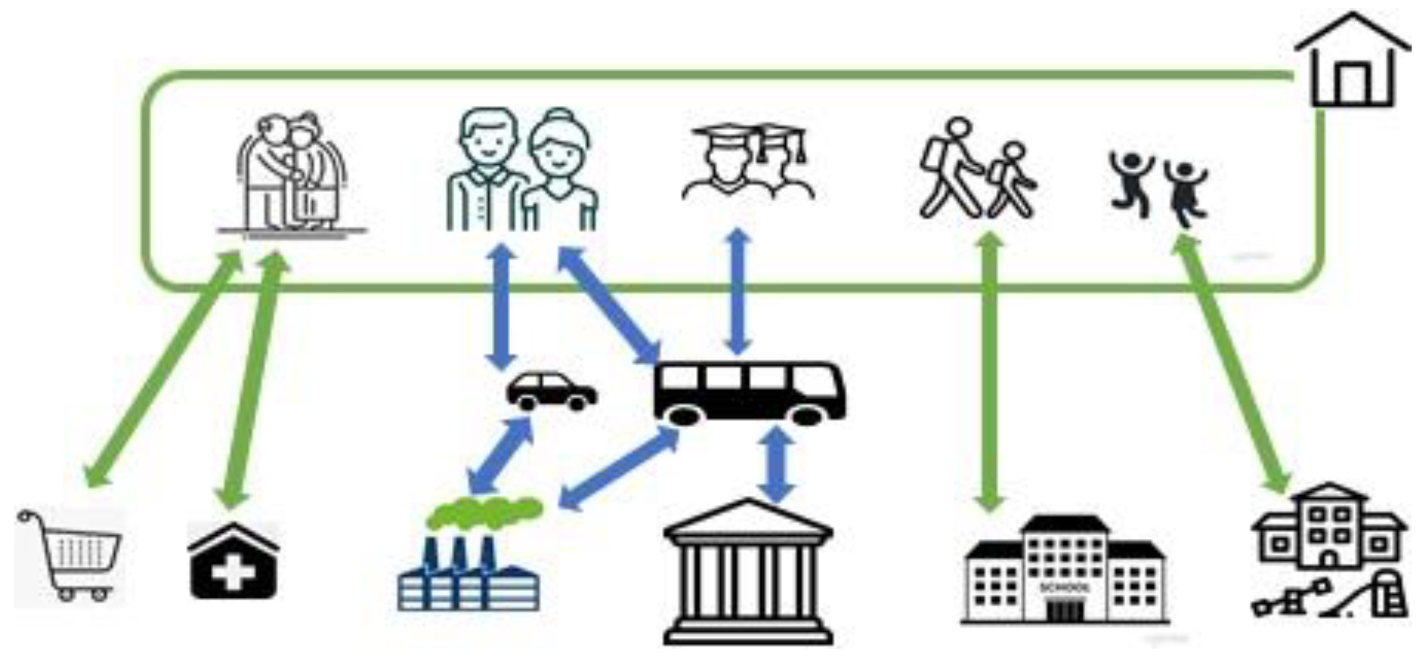
Figure 1. Social network.

Figure 2. Disease transmission.

Figure 3. Daily number of COVID-19 cases.

Figure 4. Total cases of COVID-19.

Figure 5. Parameter fitting result. Red line - average value over 50 iterations, green line – real data.

Figure 6. Forecasting total cases and evaluation of forecasting accuracy in AB time frame (a, b) and in AC time frame (c, d). Green line—real data, red line—mean (95%CI) predicted data.

Figure 7. Forecasting total cases and evaluation of forecasting accuracy MAPE in AE (a, b) and AF (c, d) time frames. Green line—real data, red line—mean (95%CI) predicted data.

Figure 8. Estimated epidemic curves of the COVID-19 outbreak under various scenarios.

Figure 9. Infection by location (a) and by age group (b).

Figure 10. Number of additional beds needed (a) and financial costs for equipment and materials (b).

Table 1. Model accuracy.

Table .	p-transmission probability	MAPE%
0-50	0.09	53
50-100	0.069	41
100-120	0.084	17
120-150	0.024	5
150-200	0.011	8
Overall		28

Table 2. Accuracy of forecasting from 51 to 65 days.

Forecasting period	5 days	10 days	15 days
MAPE%	20	42	65.7

Table 3. Impact of COVID-19 on hospitalization in the simulated scenarios.

Scenario	TotalCases	Outpatient	Hospitalized	ICU	Ventilated
BS	471,746	349,092	122,654	7,359	1,651
SC	438,610	324,571	114,039	6,842	1,535
MV	215,715	159,629	56,086	3,365	755
VS	307,381	227,462	79,919	4,795	1,076
CM	604	445	159	10	2
RS	145,044	107,757	37,287	2,294	502

Table 4. Health care workers demand in the simulated scenarios.

		BS	SC	MV	VS	CM	RS
Inpatient	Total number of health care workers	1,970	1,970	1,970	1,970	54	1,970
	Total number of cleaners	3,121	3,121	2,528	3,121	13	1,688
	Total number of ambulance personnel	4,458	4,458	3,611	4,458	18	2,412
	Total number of biomedical engineers	134	134	108	134	1	72
Laboratories	Total number of lab staff required	3	3	3	3	3	3
Laboratories	Total number of cleaners	1	1	1	1	1	1

Disclaimer/Publisher’s Note: The statements, opinions and data contained in all publications are solely those of the individual author(s) and contributor(s) and not of MDPI and/or the editor(s). MDPI and/or the editor(s) disclaim responsibility for any injury to people or property resulting from any ideas, methods, instructions or products referred to in the content.

© 2023 by the authors. Licensee MDPI, Basel, Switzerland. This article is an open access article distributed under the terms and conditions of the Creative Commons Attribution (CC BY) license (http://creativecommons.org/licenses/by/4.0/).

Copyright: This open access article is published under a Creative Commons CC BY 4.0 license, which permit the free download, distribution, and reuse, provided that the author and preprint are cited in any reuse.

MDPI Initiatives

Important Links

Choose an area of interest and we will send you notifications of new preprints at your preferred frequency.

Disclaimer