Submitted:
06 September 2023
Posted:
07 September 2023
You are already at the latest version
Abstract
Keywords:
1. Introduction
2. Construction of a Risk Assessment Index System for High-Fill Subgrade Constructions
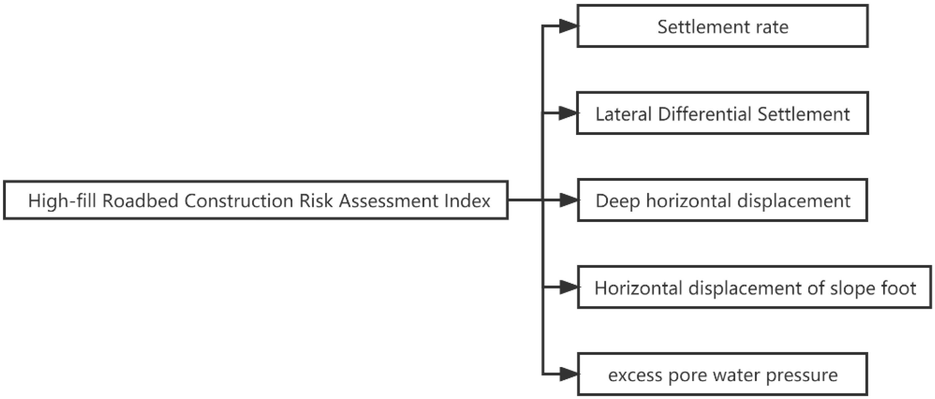
| Index | Meaning | Monitoring alert value |
|---|---|---|
| u1 | Settlement rate (mm/d) |
According to the “Technical Guidelines for Design and Construction of Highway Embankment on Soft Ground” (JTG/T D31-02-2013), the alert value of the settlement on the top surface of the fill layer should be set to 10 mm/d. |
| u2 | Lateral differential settlement (cm) | According to references [31] and [32], the maximum allowable horizontal differential settlement should be set to 7 cm. |
| u3 | Deep horizontal displacement | According to the inflection point method proposed by “Standard for Monitoring of Subgrade on Soft Ground” (GB/T 51275-2017), a danger warning is required when the displacement curve has an inflection point, and the slope after the inflection point is larger than twice the slope before the inflection point. |
| u4 | Horizontal displacement of the slope foot (mm/d) | According to the “Technical Specification for Monitoring of Highway Subgrades” (DB45/T 2364-2021), the alert value of the horizontal displacement of the slope foot should be set to 5 mm/d. |
| u5 | Excess pore water pressure (%) | According to the “Specification for Pore Pressure Measurement” (CECS55-93) and the “Code for Investigation of Geotechnical Engineering” (GB 50021-2001), the maximum allowable value of excess pore water pressure should be set to 0.6 times the overlying effective stress. Also, the index should be set to the ratio of excess pore water pressure to the maximum allowable value of excess pore water pressure at the corresponding monitoring position. |
| Risk Index | Risk Level | |||
|---|---|---|---|---|
| I | II | III | IV | |
| u1 (mm/d) | ≤7 | (7, 8.5] | (8.5, 10] | >10 |
| u2 (cm) | ≤3 | (3, 5] | (5, 7] | >7 |
| u3 (times) | ≤1.4 | (1.4, 1.7] | (1.7, 2] | >2 |
| u4 (mm/d) | ≤3.5 | (3.5, 4.25] | (4.25, 5] | >5 |
| u5 (%) | ≤0.7 | (0.7, 0.85] | (0.85, 1] | >1 |
3. Comprehensive Risk Evaluation Model Based on the Combination weighting method based on game theory
3.1. Combination weighting method based on game theory
| Scales | Meanings |
|---|---|
| 1 | i is as important as j |
| 3 | i is slightly more important than j |
| 5 | i is more important than j |
| 7 | i is even more important than j |
| 9 | i is really more important than j |
3.2. Establishment of a comprehensive risk evaluation model for the construction of a high-fill subgrade
| Type of function | Partial small membership function | Intermediate type membership function | Partial large membership function |
|---|---|---|---|
| Trapezoidal membership function |
4. Case Study
4.1. Data selection and processing
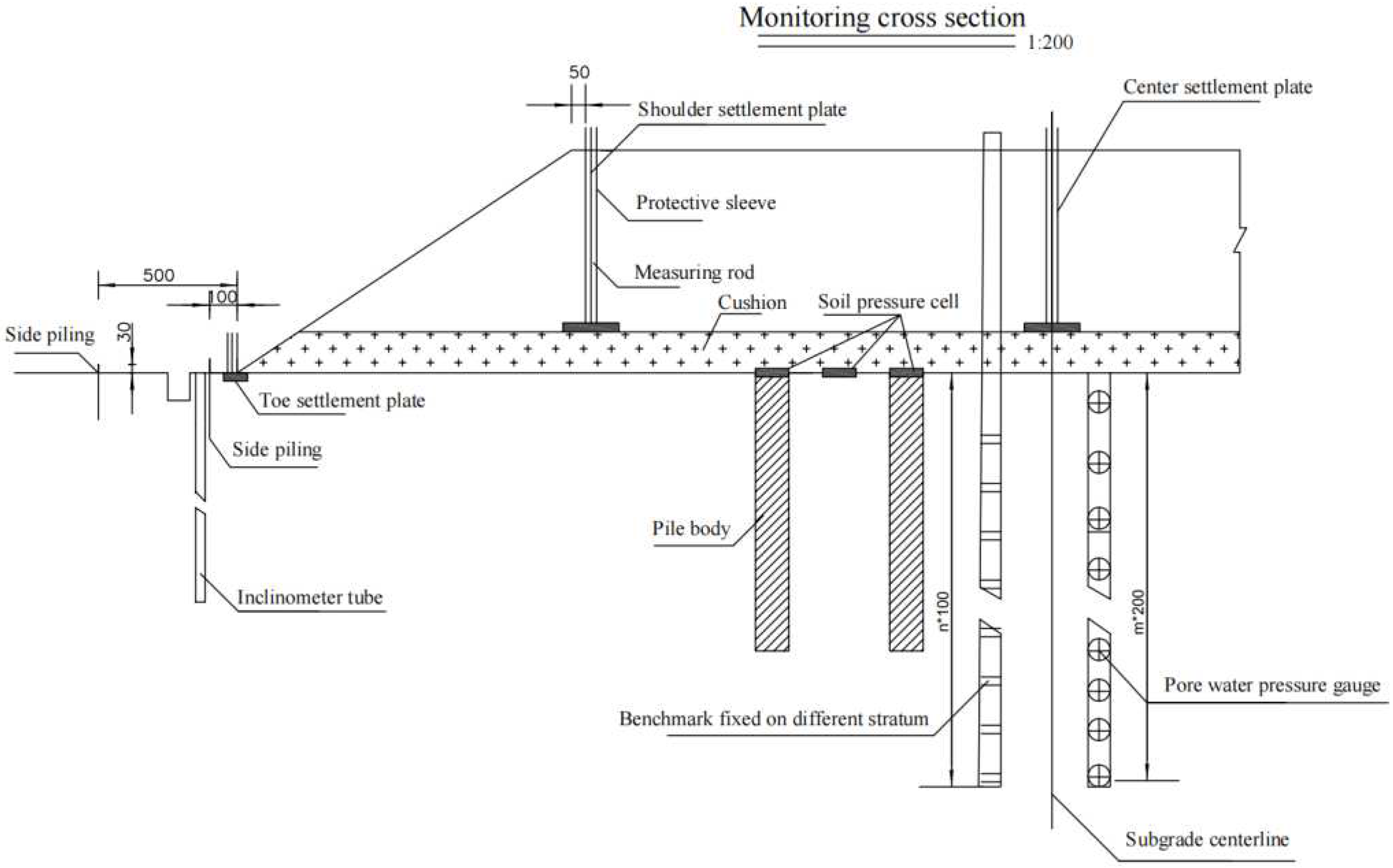
| Road section | Construction stake number | Shoulder settlement plate | Central settlement plate | Inclino-meter | Border Pile | Vibrating wire piezometer | Earth pressure cell |
|---|---|---|---|---|---|---|---|
| L1 | K27+060~ K27+707 |
4 | 2 | 3 | 3 | 3 | 3 |
| L2 | ZK31+730~ ZK31+810 |
4 | 2 | 3 | 3 | 3 | 3 |
| L3 | ZK31+830~ ZK32+100 |
4 | 2 | 2 | 3 | 3 | 3 |
| Road section |
u1 (mm/d) |
u2 (cm) |
u3 |
u4 (mm/d) |
u5 (%) |
|---|---|---|---|---|---|
| L1 | 4.333 | 6.47 | 1.9 | 0.500 | 0.541 |
| L2 | 0.717 | 2.21 | 1.5 | 0.428 | 0.560 |
| L3 | 2.667 | 3.37 | 1.6 | 0.571 | 0.209 |
| Road section | u1 | u2 | u3 | u4 | u5 |
|---|---|---|---|---|---|
| L1 | 0.165 | 0.342 | 0.789 | 0.856 | 0.386 |
| L2 | 1 | 1 | 1 | 1 | 0.373 |
| L3 | 0.269 | 0.656 | 0.938 | 0.750 | 1 |
4.2. Establishment of optimized combination weights
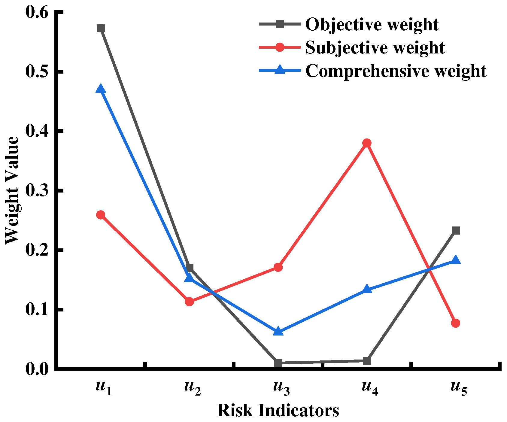
| Risk Index | u1 | u2 | u3 | u4 | u5 |
|---|---|---|---|---|---|
| Mean | 3.571 | 2.571 | 3.071 | 3.714 | 2.429 |
| A | u1 | u2 | u3 | u4 | u5 |
| u1 | 1 | 3 | 2 | 1/2 | 4 |
| u2 | 1/3 | 1 | 1/2 | 1/4 | 2 |
| u3 | 1/2 | 2 | 1 | 1/3 | 3 |
| u4 | 2 | 4 | 3 | 1 | 5 |
| u5 | 1/4 | 1/2 | 1/3 | 1/5 | 1 |
4.3. Comprehensive assessment
| Membership matrix | Evaluation index | Risk Level | |||
|---|---|---|---|---|---|
| I | II | III | IV | ||
| R1 | u1 | 0.374 | 0.626 | 0 | 0 |
| u2 | 0 | 0.653 | 0.815 | 0 | |
| u3 | 0.063 | 0.533 | 0.831 | 0 | |
| u4 | 0.700 | 0.300 | 0 | 0 | |
| u5 | 0.218 | 0.782 | 0 | 0 | |
| R2 | u1 | 0.802 | 0.198 | 0 | 0 |
| u2 | 0.231 | 0.769 | 0 | 0 | |
| u3 | 0.010 | 0.990 | 0.251 | 0 | |
| u4 | 0.678 | 0.322 | 0 | 0 | |
| u5 | 0.232 | 0.768 | 0 | 0 | |
| R3 | u1 | 0.657 | 0.343 | 0 | 0 |
| u2 | 0.090 | 0.910 | 0.109 | 0 | |
| u3 | 0.027 | 0.973 | 0.451 | 0 | |
| u4 | 0.674 | 0.326 | 0 | 0 | |
| u5 | 0.343 | 0.657 | 0 | 0 | |
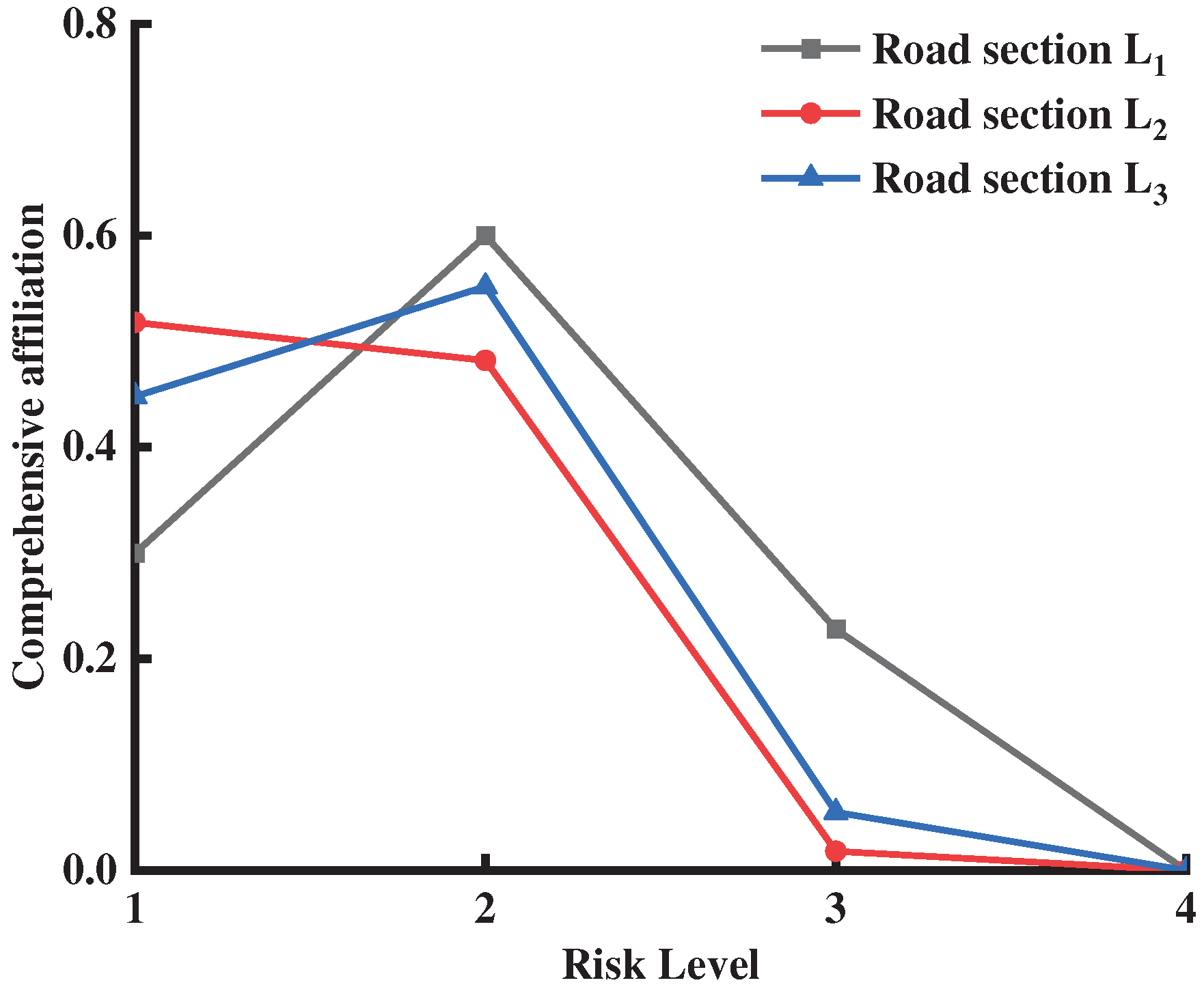
| Comprehensive membership | Risk Level | |||
|---|---|---|---|---|
| I | II | III | IV | |
| B1 | 0.313 | 0.609 | 0.175 | 0 |
| B2 | 0.545 | 0.455 | 0.016 | 0 |
| B3 | 0.477 | 0.523 | 0.045 | 0 |
| Road section | AHP method | Entropy method |
|---|---|---|
| L1 | [0.390 0.501 0.234 0] | [0.275 0.662 0.147 0] |
| L2 | [0.511 0.489 0.043 0] | [0.562 0.438 0.002 0] |
| L3 | [0.468 0.532 0.089 0] | [0.481 0.519 0.023 0] |
| Road section | Combined method | AHP method | Entropy method |
|---|---|---|---|
| L1 | 78.145 | 78.467 | 77.952 |
| L2 | 88.017 | 86.218 | 88.972 |
| L3 | 85.335 | 83.701 | 86.193 |
4.4. Model stability analysis
| Random number | Error index | Noise amplitude (%) | |||||
|---|---|---|---|---|---|---|---|
| 5 | 10 | 20 | 30 | 40 | 50 | ||
| 1 | MAE | 0.545 | 1.057 | 1.742 | 3.289 | 5.661 | 7.964 |
| MAPE | 0.616 | 1.191 | 1.967 | 3.777 | 6.663 | 9.685 | |
| 2 | MAE | 0.410 | 0.671 | 1.363 | 2.490 | 4.354 | 6.182 |
| MAPE | 0.465 | 0.760 | 1.574 | 2.871 | 5.050 | 7.345 | |
| 3 | MAE | 0.531 | 0.996 | 1.821 | 3.187 | 5.287 | 7.512 |
| MAPE | 0.598 | 1.126 | 2.104 | 3.721 | 6.275 | 9.156 | |
| 4 | MAE | 0.287 | 0.590 | 1.258 | 2.385 | 4.616 | 6.764 |
| MAPE | 0.319 | 0.657 | 1.482 | 2.864 | 5.577 | 8.388 | |
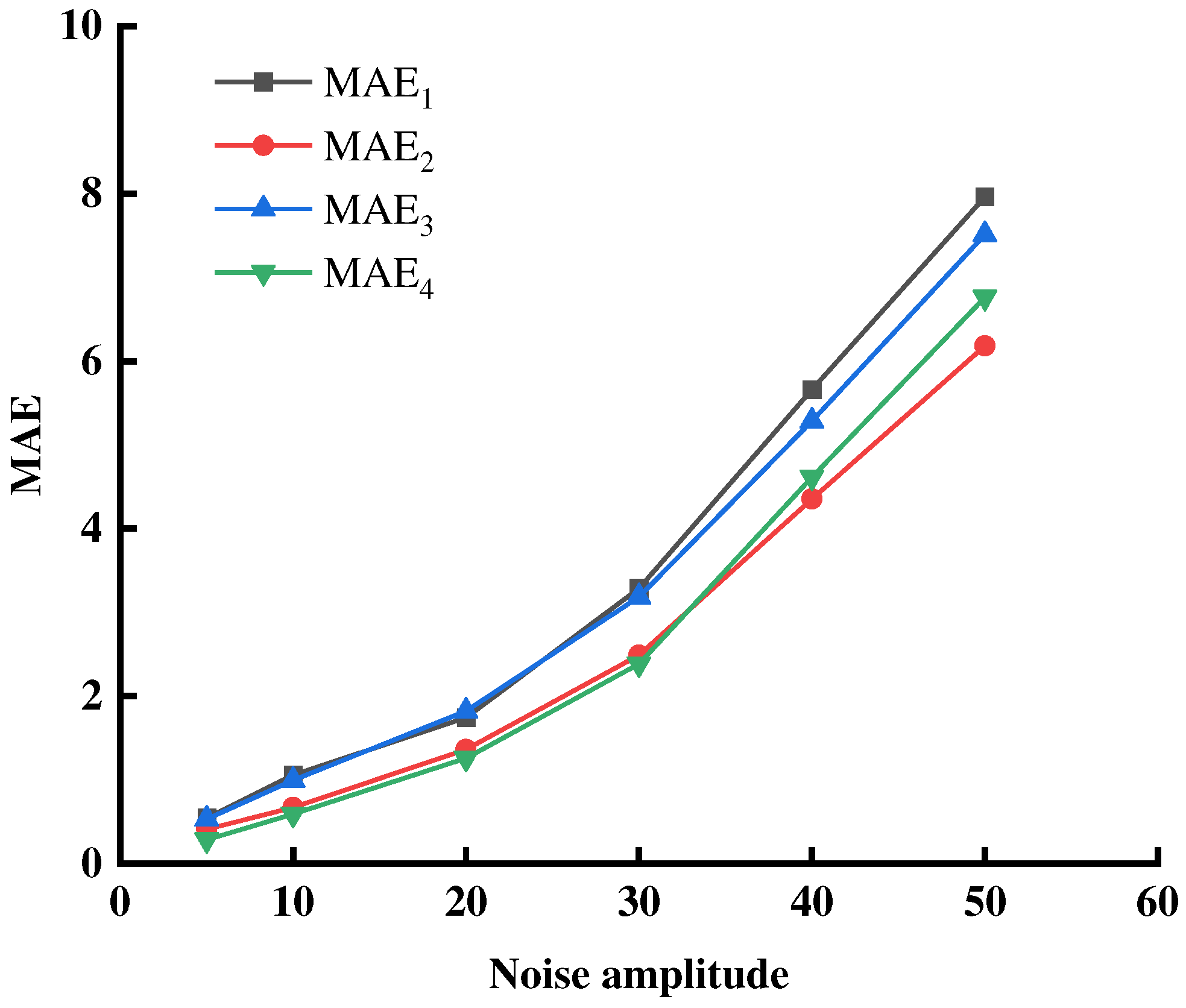
5. Conclusions
- (1)
- Combining the combination weighting method of Nash equilibrium thought in Game theory, the centralized unification of subjective and objective weighting of indicators is realized. This method considers the empirical judgments of experts on indicators and the objective attributes of evaluation indicators, avoiding the one-sidedness caused by single subjective or objective weighting.
- (2)
- The trapezoidal membership function was conducted as the membership function to evaluate each indicator level, and the fuzzy comprehensive evaluation method using the maximum membership principle and weighted average principle ensured the effectiveness of the evaluation results.
- (3)
- Applying the monitoring data of Zhitong Expressway for the evaluation model, it was found that the three methods yielded similar safety rating results for each section. The combined weighted evaluation model can correct the evaluation result error caused by a single weight, and the monitoring index error is within 20%.
- (4)
- The evaluation method proposed in this study provides a quick reference for construction safety management and safety warning. It can avoid information lag caused by the manual processing and analysis of monitoring data. However, the subgrade monitoring indexes will change for different engineering situations, so the universality and promotion value should be investigated in future cases.
- (5)
- The index requirements for high-fill subgrades of the reference specification in this study apply to non-specialized soil high-fill subgrades and high-fill subgrades on soft soil foundations, and other special soil subgrades can be borrowed for reference. However, their applicability needs to be further demonstrated.
Author Contributions
Funding
Institutional Review Board Statement
Informed Consent Statement
Data Availability Statement
Acknowledgments
Conflicts of Interest
References
- Chen, D.; Ling, J.; Li, D.; Zheng, C. Monitoring and evaluating techniques of highway subgrade safety in the operation period. Road Materials and Pavement Design 2017, 18(sup3), 215–225. [Google Scholar] [CrossRef]
- Le Kouby, A.; Guimond-Barrett, A.; Reiffsteck, P.; Pantet, A.; Mosser, J.-F.; Calon, N. Improvement of existing railway subgrade by deep mixing. European Journal of Environmental and Civil Engineering 2020, 24(8), 1229–1244. [Google Scholar] [CrossRef]
- Lei, G.; Qiu-Yue, Z.; Xiang-Juan, Y.; Zhi-Hui, C. Analysis and model prediction of subgrade settlement for Linhai highway in China. Electronic Journal of Geotechnical Engineering 2014, 19, 11–21. [Google Scholar]
- Jia, L.; Guo, J.; Yao, K. In Situ Monitoring of the Long-Term Settlement of High-Fill Subgrade. Advances in Civil Engineering 2018, 2018, 1–9. [Google Scholar] [CrossRef]
- Bakhat, R.; Rajaa, M. Risk Assessment of a Wind Turbine Using an AHP-MABAC Approach with Grey System Theory: A Case Study of Morocco. Mathematical Problems in Engineering 2020, 2020, 1–22. [Google Scholar] [CrossRef]
- Wu, Z.; Shen, R. Safety Evaluation Model of Highway Construction based on Fuzzy Grey Theory. Procedia Engineering 2012, 45, 64–69. [Google Scholar] [CrossRef]
- Lin, C. J.; Zhang, M.; Li, L. P.; Zhou, Z. Q.; Liu, S.; Liu, C.; Li, T. Risk Assessment of Tunnel Construction Based on Improved Cloud Model. Journal of Performance of Constructed Facilities 2020, 34(3). [Google Scholar] [CrossRef]
- Luo, D.; Li, H.; Wu, Y.; Li, D.; Yang, X.; Yao, Q. Cloud model-based evaluation of landslide dam development feasibility. PLOS ONE 2021, 16(5), e0251212. [Google Scholar] [CrossRef]
- Wang, R.; Zhao, Q.; Sun, H.; Zhang, X.; Wang, Y. Risk Assessment Model Based on Set Pair Analysis Applied to Airport Bird Strikes. Sustainability 2022, 14(19), 12877. [Google Scholar] [CrossRef]
- Zhang, L.; Li, H. Construction Risk Assessment of Deep Foundation Pit Projects Based on the Projection Pursuit Method and Improved Set Pair Analysis. Applied Sciences 2022, 12(4), 1922. [Google Scholar] [CrossRef]
- Chen, W.; Zhang, G.; Jiao, Y.; Wang, H. Unascertained Measure-Set Pair Analysis Model of Collapse Risk Evaluation in Mountain Tunnels and Its Engineering Application. KSCE Journal of Civil Engineering 2020, 25(2), 451–467. [Google Scholar] [CrossRef]
- Zhang, G.; Wang, C.; Jiao, Y.; Wang, H.; Qin, W.; Chen, W.; Zhong, G. Collapse Risk Analysis of Deep Foundation Pits in Metro Stations Using a Fuzzy Bayesian Network and a Fuzzy AHP. Mathematical Problems in Engineering 2020, 2020, 1–18. [Google Scholar] [CrossRef]
- Wang, J.; Ma, C.; Wang, S.; Lu, X.; Li, D. Risk Assessment Model and Sensitivity Analysis of Ordinary Arterial Highways Based on RSR-CRITIC-LVSSM-EFAST. Sustainability 2022, 14(23), 16096. [Google Scholar] [CrossRef]
- Gebrehiwet, T.; Luo, H. Risk Level Evaluation on Construction Project Lifecycle Using Fuzzy Comprehensive Evaluation and TOPSIS. Symmetry 2018, 11(1), 12. [Google Scholar] [CrossRef]
- Yu, X.; Suntrayuth, S.; Su, J. A Comprehensive Evaluation Method for Industrial Sewage Treatment Projects Based on the Improved Entropy-TOPSIS. Sustainability 2020, 12(17), 6734. [Google Scholar] [CrossRef]
- Li, Q.; Zhou, J.; Feng, J. Safety Risk Assessment of Highway Bridge Construction Based on Cloud Entropy Power Method. Applied Sciences 2022, 12(17), 8692. [Google Scholar] [CrossRef]
- Alawad, H.; Kaewunruen, S.; An, M. A Deep Learning Approach Towards Railway Safety Risk Assessment. IEEE Access 2020, 8, 102811–102832. [Google Scholar] [CrossRef]
- Isah, M. A.; Kim, B.-S. Assessment of Risk Impact on Road Project Using Deep Neural Network. KSCE Journal of Civil Engineering 2021, 26(3), 1014–1023. [Google Scholar] [CrossRef]
- Lai, C.; Chen, X.; Chen, X.; Wang, Z.; Wu, X.; Zhao, S. A fuzzy comprehensive evaluation model for flood risk based on the combination weight of game theory. Natural Hazards 2015, 77(2), 1243–1259. [Google Scholar] [CrossRef]
- Li, H.; Chen, L.; Tian, F.; Zhao, L.; Tian, S. Comprehensive Evaluation Model of Coal Mine Safety under the Combination of Game Theory and TOPSIS. Mathematical Problems in Engineering 2022, 2022, 1–15. [Google Scholar] [CrossRef]
- Tang, J.; Wang, D.; Ye, W.; Dong, B.; Yang, H. Safety Risk Assessment of Air Traffic Control System Based on the Game Theory and the Cloud Matter Element Analysis. Sustainability 2022, 14(10), 6258. [Google Scholar] [CrossRef]
- Hegde, J.; Rokseth, B. Applications of machine learning methods for engineering risk assessment – A review. Safety Science 2020, 122, 104492. [Google Scholar] [CrossRef]
- Islam, M. S.; Nepal, M. P.; Skitmore, M.; Attarzadeh, M. Current research trends and application areas of fuzzy and hybrid methods to the risk assessment of construction projects. Advanced Engineering Informatics 2017, 33, 112–131. [Google Scholar] [CrossRef]
- Bao, X.; Li, H. Construction Risk Analysis of Subgrade Engineering in Perilous Mountainous Areas. Journal of Railway Engineering Society 2022, 39(07), 109-115+121. [Google Scholar]
- Guo, Q.; Li, Y.; Meng, X.; Guo, G.; Lv, X. Instability risk assessment of expressway construction site above an abandoned goaf: a case study in China. Environmental Earth Sciences 2019, 78(20), 588. [Google Scholar] [CrossRef]
- Zhang, Q.; Su, Q.; Liu, B.; Pei, Y.; Zhang, Z.; Chen, D. Comprehensive performance evaluation of high embankments in heavy-haul railways using an improved extension model with attribute reduction algorithm. Journal of Intelligent & Fuzzy Systems 2023, 44(2), 2673–2692. [Google Scholar] [CrossRef]
- Taskiran, T.; Fidan, A. A. Investigation of the Parameters Affecting the Stability of Unsaturated Soil Slope Subjected to Rainfall. TEKNIK DERGI 2019, 30(5), 9483–9506. [Google Scholar]
- Wu, D.; Wang, Y.; Zhang, F.; Qiu, Y. Influences of Pore-Water Pressure on Slope Stability considering Strength Nonlinearity. Advances in Civil Engineering 2021, 2021, 8823899. [Google Scholar] [CrossRef]
- Li, Z.; Guan, C.; Han, M.; Jia, J.; Liu, L.; Li, W. Estimation of Settlement in Loess-Filled Subgrade with Consideration of Lateral Deformation. Arabian Journal for Science and Engineering 2022, 47(4), 4713–4729. [Google Scholar] [CrossRef]
- Raja, K.; Vishnuvardhan, K.; Venkatachalam, S.; Richard, P. D.; Ramu, T.; RamKumar, S. Strength and settlement of subgrade soil in southern part of Kangeyam block. Materials Today: Proceedings 2022, 65, 1930–1938. [Google Scholar] [CrossRef]
- Yan, Q.; Zhi, X.; Liu, B. standard of differential settlement for highway subgrade. Journal of Chang’an University(Natural Science Edition) 2013, 33(02), 16–21. [Google Scholar]
- Xingxin, C.; Xuancang, W.; Zhiwei, G. Control criterion of subgrade differential settlement based on pavement damage response. Journal of Chang’an University(Natural Science Edition) 2010, 30(05), 31–34. [Google Scholar]
- Hummel, J. M.; Bridges, J. F. P.; Ijzerman, M. J. Group Decision Making with the Analytic Hierarchy Process in Benefit-Risk Assessment: A Tutorial. The Patient - Patient-Centered Outcomes Research 2014, 7(2), 129–140. [Google Scholar] [CrossRef] [PubMed]
- Abedian, M.; Amindoust, A.; Maddahi, R.; Jouzdani, J. A Nash equilibrium based decision-making method for performance evaluation: a case study. Journal of Ambient Intelligence and Humanized Computing 2021, 13(12), 5563–5579. [Google Scholar] [CrossRef]
- He, H.; Tian, C.; Jin, G.; An, L. An Improved Uncertainty Measure Theory Based on Game Theory Weighting. Mathematical Problems in Engineering 2019, 2019, 1–8. [Google Scholar] [CrossRef]
- Koulinas, G. K.; Marhavilas, P. K.; Demesouka, O. E.; Vavatsikos, A. P.; Koulouriotis, D. E. Risk analysis and assessment in the worksites using the fuzzy-analytical hierarchy process and a quantitative technique – A case study for the Greek construction sector. Safety Science 2019, 112, 96–104. [Google Scholar] [CrossRef]
- Wang, G.; Liu, Y.; Hu, Z.; Lyu, Y.; Zhang, G.; Liu, J.; Liu, Y.; Gu, Y.; Huang, X.; Zheng, H.; Zhang, Q.; Tong, Z.; Hong, C.; Liu, L. Flood Risk Assessment Based on Fuzzy Synthetic Evaluation Method in the Beijing-Tianjin-Hebei Metropolitan Area, China. Sustainability 2020, 12(4), 1451. [Google Scholar] [CrossRef]
Disclaimer/Publisher’s Note: The statements, opinions and data contained in all publications are solely those of the individual author(s) and contributor(s) and not of MDPI and/or the editor(s). MDPI and/or the editor(s) disclaim responsibility for any injury to people or property resulting from any ideas, methods, instructions or products referred to in the content. |
© 2023 by the authors. Licensee MDPI, Basel, Switzerland. This article is an open access article distributed under the terms and conditions of the Creative Commons Attribution (CC BY) license (http://creativecommons.org/licenses/by/4.0/).


