1. Introduction

2. Problem descriptions

2.1. Target ship and flow control fins

The base DNN used for predicting wake distribution and resistance is trained using data from the author’s previous paper. A relatively substantial amount of data used for training the DNN model comes from a 1,000 TEU containership constructed by Daesun Shipbuilding & Engineering Co. Ltd. This was associated with the presence of reliable CFD data. A model with a scale ratio $\lambda =30.56$ was selected for numerical simulation. The data used for the transfer learning model consists of different-sized vessels: 2,500 TEU and 3,600 TEU (KCS; KRISO Containership) containerships. For these ships, models with each scale ratio of $\lambda =27.2$ and $\lambda =31.6$ were considered. The principal dimensions of target hulls and propellers are given in Table 1. Figure 1 presents the three-dimensional views of target hull forms and propellers.

Table 1. Principal particulars of 1,000TEU containership.

Table 1. Principal particulars of 1,000TEU containership.

Class	Designation	Symbol (unit)	Full-scale ship
1,000 TEU	Length bet. Perpendicular	$L_{PP}$ (m)	137.5
	Breadth	$B$ (m)	23.6
	Draft	$T$ (m)	7.4
	Block coefficient	$C_B$	0.595
	Propeller Diameter	$DIA$ (m)	5.5
2,500 TEU	Length bet. Perpendicular	$L_{PP}$ (m)	185.0
	Breadth	$B$ (m)	32.26
	Draft	$T$ (m)	10.0
	Block coefficient	$C_B$	0.640
	Propeller Diameter	$DIA$ (m)	6.8
3,600 TEU	Length bet. Perpendicular	$L_{PP}$ (m)	230.0
	Breadth	$B$ (m)	32.2
	Draft	$T$ (m)	10.8
	Block coefficient	$C_B$	0.651
	Propeller Diameter	$DIA$ (m)	7.9

Figure 1. 3D volumetric views of target hulls and propellers: (a) 1,000 TEU; (b) 2,500 TEU; (c) 3,600 TEU.

Figure 1. 3D volumetric views of target hulls and propellers: (a) 1,000 TEU; (b) 2,500 TEU; (c) 3,600 TEU.

The Flow Control Fin (FCF) used in this study is in rectangular shape with two rounded corners (see Figure 2). The dimensions of full-scale FCF were 1.30 m long, 0.37m high, and 0.03m thick. When normalized by the propeller diameter $D$, these correspond to $0.236D$ (length) × $0.0673D$ (height) × $0.00545D$ (thickness). Generally, FCFs are attached in pair(s) at the same locations on the port and starboard sides. The design variables for the FCF are the longitudinal and vertical positions of FCF, inclination angle, and hull-form information. Here, the position of the FCF is located at the midpoint of the baseline, and the angle of inclination refers to the angle between the FCF baseline and the ship baseline. The hull-form information applies the derivatives representing the gradient of each tangent at the midpoint of the FCF in the directions of the station, waterline, and buttock line. In more detail, when the derivative is small in the station direction, it indicates that when observing the hull-form in the body plan, the shape resembles a V type. Similarly, when the derivatives are small in the waterline and buttock line directions, they represent hull-form that changes smoothly in the half-breadth and shear plan, respectively.

Figure 2. Geometry of FCF.

Figure 2. Geometry of FCF.

Indeed, even within the same type of vessel, differences in main particulars, hull-form, and the position of the FCF can result in variations in the characteristics of the propeller inflow velocity distribution. Figure 3 illustrates the distribution of the viscous resistance coefficient and the standard deviation of axial velocity distribution based on derivatives in the waterline and buttock line directions. The orange symbols represent the viscosity resistance coefficients and standard deviation for 1,000 TEU, the green symbols for 2,500 TEU, and the blue symbols for 3,600 TEU. Transfer learning was employed to predict values with varying characteristics across different ship sizes.

Figure 3. Features distribution for each containership: (a) distribution of viscous resistance coefficient; (b) standard deviation of axial velocity distribution.

Figure 3. Features distribution for each containership: (a) distribution of viscous resistance coefficient; (b) standard deviation of axial velocity distribution.

2.2. CFD simulation to obtain training data

In this study, 693 datasets were prepared by the CFD analysis to train, validate, and test the base DNN model. Each data corresponded to a combination of design parameters, including 11 longitudinal positions $\left(3.0\le x/St.\le 4.0,∆x/St.=0.1\right)$ $\times$ vertical positions $\left(0.135\le z/T\le 0.405,∆z/T=0.0135\right)$ $\times 3$ inclination angles $(\alpha =19°,20°,21°)$. Here, $St.$ Refers to the station length, which is 1/20 of the length between perpendicular $L_{PP}$. Around 150 target datasets for 2,500 TEU and 3,600 TEU were obtained through CFD analysis for transfer learning. The target datasets were randomly selected within the same longitudinal and vertical position ranges as the source datasets. Similarly, the inclination angles were also randomly specified.

It is necessary to emphasize the importance of automation in such preprocessing steps as modeling and mesh generation, as it significantly enhances the overall computational efficiency for the entire set of 843 simulation cases. The processes including three-dimensional modeling of hull-forms with varying FCF positions, mesh generation, and creation of CFD setups was carried out using OptHull^® software, a professional hull form design software. Then, the commercial CFD S/W STAR-CCM+ was configured and the numerical analysis were automatically controlled by an in-house javascript code. By using a 140 CPU (Intel Xeon 2.6GHz)-parallel computing cluster, approximately 419 hours were required to complete the preparation of data for the 843 simulations.

2.2.1. Governing equations

The STAR-CCM+ v.15.06 was used for the CFD analysis of the flow around the ship. The governing equations consist of the continuity equation for mass conservation and the Reynolds-Averaged Navier-Stokes (RANS) equations for momentum and energy conservation. These equations are given in the following tensor notation;

$$\frac{\partial U_i}{\partial x_i}=0$$

(1)

$$\frac{\partial U_i}{\partial t}+\rho U_l\frac{\partial U_i}{\partial x_l}=-\frac{\partial p}{\partial x_i}+\frac{\partial }{\partial x_l}\left(\mu \frac{\partial U_i}{\partial x_l}-\rho \overline{u_i{u}_l}\right)+\rho g_i$$

(2)

where $U_i=\left(U,V,W\right)$ is the velocity component in $x_i=\left(x,y,z\right)$ direction, while $p,\rho ,\mu ,-\overline{u_i{u}_l}$ and $g_i$ are the static pressure, fluid density, absolute viscosity of fluid, Reynolds stress, and gravitational acceleration in the $x_i$-direction, respectively.

The Reynolds stress turbulent model, being excellent in resolving bilge vortex and capable of high-accuracy prediction of flow around the ship [10], was employed in the numerical analysis. The transport equation for the Reynolds stress is described as follows;

$$\frac{D\overline{u_i^{’}{u}_j^{’}}}{Dt}=D_{ij}+G_{ij}-\frac{2}{3}{\delta }_{ij}\epsilon +PS$$

(3)

where ${\delta }_{ij}$ is the Kronecker delta and $D_{ij}$, $G_{ij}$ and $PS$ correspond to the diffusion, production, and pressure strain terms which are expressed as follows;

$$D_{ij}=\frac{\partial }{\partial x_l}\left(C_k\frac{k^2}{\epsilon }\frac{\partial \overline{u_i{u}_j}}{\partial x_l}+\nu \frac{\partial \overline{u_i{u}_j}}{\partial x_l}\right)$$

(4)

$$G_{ij}=-\left(\overline{u_i{u}_l}\frac{\partial U_j}{\partial x_l}+\overline{u_j{u}_l}\frac{\partial U_j}{\partial x_l}\right)$$

(5)

$$PS=-C_1\frac{\epsilon }{k}\left(\overline{u_i{u}_j}-\frac{2}{3}{\delta }_{ij}k\right)-C_2\left(G_{ij}-\frac{2}{3}{\delta }_{ij}{G}_k\right)$$

(6)

Here, $C_k$, $C_1$ and $C_2$ are turbulent model constants. Additionally, $k$ and $\epsilon$ respectively represent turbulent kinetic energy and dissipation rate.

2.2.2. Computational domain and boundary conditions

Figure 4 illustrates the computational domain, which is rectangular, set within the range of $-2.5L_{PP}<x<L_{PP},0<y<1.5L_{PP}$, and $-1.5L_{PP}<z<0$. Since the computational domain is symmetric with respect to the center plane $(y=0)$, only half domain was considered. In addition, a double-body simulation, in which the underwater hull was mirrored with respect to the free surface $(z=0)$, was performed for all cases. This approach allows the neglect of wave generation by the ship hull and the resulting wave-making resistance. However, due to the deep submergence of the FCF, which prevents its influence on the free surface, complex issues in analyzing the various effects of FCF design on the flow field are avoided. The double-body simulation significantly reduces the computational time by omitting computationally intensive free-surface calculations, which is crucial for this study encompassing various test cases. The boundary conditions for the computational domain surfaces shown in Figure 4 are summarized in Table 2.

Figure 4. Computational domain for double-body simulation.

Figure 4. Computational domain for double-body simulation.

Table 2. Boundary conditions for Figure 6.

Table 2. Boundary conditions for Figure 6.

Boundary surface	Type
Inlet	Velocity inlet
Outlet	Pressure outlet
Top, Bottom, Side, Centerplane	Symmetry
Ship	Wall

2.2.3. Uncertainty analysis in CFD verification methodology

The validation of CFD analysis used to acquire 839 data points is unavoidable. In this study, a double body analysis was conducted to reduce data collection time. As a result, validation with model tests could not be carried out. Therefore, the verification of the grid system used in the analysis was performed following the procedures and guidelines recommended by ITTC [11]. To verify specific parameters used in the CFD analysis, numerical error and uncertainty of the simulation are evaluated. A parameter convergence study is performed by varying the $ith$ input parameter $△x_{G,i}$ while keeping all other parameters constant, using multiple solutions with systematic parameter refinement. The input parameter is varied based on the refinement ratio defined in Equation (7).

$$r_G=△x_{G,2}/△x_{G,1}=△x_{G,3}/△x_{G,2}=△x_{G,m}/△x_{G,m-1}=\sqrt{2}$$

(7)

At least three values of the input parameter are required for evaluating convergence, and the convergence ratio is defined as Equation (8).

$$R_G={\epsilon }_{G,21}/{\epsilon }_{G,32}$$

(8)

Here, ${\epsilon }_G$ represents the difference in simulation solutions and is defined as the changes between the medium-fine ${\epsilon }_{G,21}={\widehat{S}}_{G,2}-{\widehat{S}}_{G,1}$ and coarse-medium ${\epsilon }_{G,32}={\widehat{S}}_{G,3}-{\widehat{S}}_{G,1}$. The convergence conditions are defined into three categories based on the convergence ratio as follows.

$$\begin{gathered} \left(i\right)\mathrm{Monotonic}\mathrm{convergence}\text{: }0<R_G<1 \\ \left(ii\right)\mathrm{Oscillatory}\mathrm{convergence}\text{: }{R}_G<0 \\ \left(iii\right)\mathrm{Divergence}\text{: }{R}_G>1 \end{gathered}$$

(9)

In case $\left(i\right)$, the generalized Richardson Extrapolation (RE) method is employed to estimate the numerical error and uncertainty. In case $\left(ii\right)$, numerical uncertainty is estimated using the following equation.

$$U_G=\frac{1}{2}\left(S_U-S_L\right)$$

(10)

Here, $S_U$ and $S_L$ represent the maximum and minimum values among the oscillating trends in the analysis results. In case $\left(iii\right)$, it is not possible to estimate numerical error and uncertainty since the analysis results exhibit a diverging tendency.

Subsequently, detailed explanations for the numerical error (${\delta }_{{RE}_G}^{*}$) and uncertainty ($U_G$) calculated through the generalized RE method are based on the ITTC Recommended Procedures and Guidelines for Uncertainty Analysis. In this study, the estimation results for numerical error and uncertainty of the grid system used in data acquisition through simulations are thoroughly described in Section 4.

3. Methodology

3.1. Deep Neural Network (DNN)

A deep Neural Network is a supervised learning technique that involves training and predicting based on input and output data. The number of hidden layers and the number of neurons in each layer connecting input and output data are determined according to the designer’s needs. The weights between layers are initialized and then continuously adjusted during the training process [12]. Figure 5 illustrates the general structure of a DNN, where $\left\{x_1,x_2,\dots ,x_d\right\}$ represents input data. The outputs of each neuron in the first and second hidden layers are calculated using the following equations;

$$h_i^l=f\left(b_l+\sum _{i=1}^n{W}_i{x}_i\right)$$

(11)

$$h_i^{j+1}=f\left(b_{j+1}+\sum _{i=1}^m{w}_i^j{h}_i^j\right),j\ge 1$$

(12)

Here, $f$ represents the activation function, $b$ stands for bias, $W$ and $w$ represent the weights of neurons in the input layer and hidden layer, respectively. Furthermore, $x$ represents the normalized input value of the input layer, and $h$ is the output of neurons in the hidden layer. The final output of the last output layer is calculated in the same way as the output of the hidden layer. The calculated output value of the DNN model is then used to compute the loss function by comparing it with the actual values. Subsequently, an optimization algorithm is used to minimize the loss function and adjust the values of weights and biases. In this study, hyperparameters such as batch size, epochs, and learning rate were determined using the grid search cross-validation method. Table 3 represents the basic configuration of the hidden layers, activation function, and optimizer used for applying the grid search.

Figure 5. The general architecture of the DNN model.

Figure 5. The general architecture of the DNN model.

Table 3. Hyper-parameters of the ANN.

Table 3. Hyper-parameters of the ANN.

Layers	Neurons	Activation function	Optimizer
1st hidden layer	11	ReLU	Adam
2nd hidden layer	22
3rd hidden layer	44
4th hidden layer	66
5th hidden layer	89

In this study, the DNN was employed to predict the axial velocity distribution in the propeller plane based on the input design variables of the Flow Control Fin (FCF). Thus, the input for the DNN consisted of the design variables $\left[x/st.,z/T,AoA,{\left(dy/dz\right)}_x,{\left(dy/dx\right)}_z,{\left(dz/dx\right)}_y\right]$, and the flow distribution became the outputs. Here, the angle of attack ($AoA$) was defined as the angle between the local streamline for the baseline hull without the FCF and the baseline of FCF. ${\left(dy/dz\right)}_x,{\left(dy/dx\right)}_z$, and ${\left(dz/dx\right)}_y$ represent the derivatives of the station line (constant $x$), waterline (constant $z$), and buttock line (constant $y$), respectively. These derivatives indicate the inclinations of the hull in each direction relative to the center point where the FCF is attached. In order to enhance the training efficiency, it was essential to align the dimensions of the neural network’s input and output as closely as possible without compromising the detailed representation of the velocity distribution. To obtain the Fourier series coefficients for the axial velocity distribution in the form of $73\times 8$ polar array (Figure 6) of the propeller plane, harmonic analysis was performed. Specifically, the circumferential distribution of the axial velocity $V_x\left(\phi \right)$ was expressed using a Fourier series up to the 10th order for eight radial positions within the range $0.3R<r<1.0R(\Delta r=0.1R)$.

$$V_x\left(\phi \right)=A\left(0\right)+\sum _{i=1}^{10}\left\{A\left(i\right)\cos \left(i\phi \right)+B\left(i\right)\mathrm{s}\mathrm{i}\mathrm{n}\left(i\phi \right)\right\}$$

(13)

The symmetry of the wake flow distribution makes the sine coefficients $B\left(i\right)=0$, resulting in the utilization of the remaining $11\times 8$ cosine coefficients as the output of the base DNN model. This Fourier analysis preprocessing was found to improve training efficiency compared to cases without preprocessing. The 693 source datasets used for the base DNN model were divided into 415 training sets, 139 validation sets, and 139 test sets. When individual data sizes significantly differ, the training often fails. To mitigate this, all data was normalized using a Min-Max scaler to ensure sizes ranged from 0 to 1.

Figure 6. Preprocessing of output data for the neural network: (a) bisecting the propeller plane; (b) harmonic analysis.

Figure 6. Preprocessing of output data for the neural network: (a) bisecting the propeller plane; (b) harmonic analysis.

3.2. Transfer Learning (TL)

The machine learning algorithms of the data-centric learning method assume that they are trained by the same distribution of train and test datasets [13]. However, in real-world applications, this assumption may not hold. When the dataset changes, machine learning algorithms need to be retrained based on a substantial amount of newly collected training data, which can be time-consuming and costly [14]. To address these issues, transfer learning can be applied, allowing efficient learning with a small amount of new data. Transfer learning involves transferring the weights of a pre-trained neural network model to a new neural network for learning, thereby facilitating the construction of a model with a small amount of newly applied data [15]. The main objective of this study is to apply Deep Neural Networks (DNN) and Transfer Learning (TL) for estimating viscous resistance and wake distribution on various sizes of container ships using the position of flow control fin and hull-form information as input features. Figure 7 provides a brief overview of how transfer learning is applied.

Figure 7. Overview of the transfer learning.

Figure 7. Overview of the transfer learning.

First, the base DNN model is trained and validated using the source dataset (1,000 TEU). Then, a new model is reconfigured (retrained and validated) based on a subset of the target dataset (2,500 TEU and 3,600 TEU), where the knowledge from the base DNN model is transferred. The remaining part of the target dataset is used in the testing phase of the reconfigured model.

3.3. Model application details

Figure 8 illustrates the structure of the algorithm for predicting viscous resistance and wake distribution of new sizes of container ships using transfer learning.

Figure 8. Workflow of transfer learning.

Figure 8. Workflow of transfer learning.

In this study, the source dataset used for training and validation of the base DNN model consists of viscous resistance and wake characteristics based on the flow control fin applied to a 1,000 TEU container ship. When training the DNN model, there are various hyperparameters that the designer needs to set, including batch size, the number of epochs, and the learning rate. The choice of the batch size used in mini-batch gradient descent affects the learning speed and the tracking of the global minimum point of the cost function. The number of epochs, which indicates how many times the entire dataset is iterated over during training, can lead to issues of overfitting and underfitting. Furthermore, selecting an appropriate optimizer and the corresponding learning rate is crucial based on the learning model and dataset used. To optimize these various hyperparameters, a grid search cross-validation method was applied, which involves exploring the optimal parameters by combining multiple settings specified by the designer. The loss function for optimizing the hyperparameters was the Mean Square Error (MSE). The base DNN model constructed with the optimal hyperparameters was then used to evaluate the learning performance on the test dataset.

Using the well-constructed base DNN model as a foundation, transfer learning was applied to create a restructured DNN model for knowledge transfer to 2,500 TEU and 3,600 TEU (KCS) as target datasets. For the reconstruction of the model through transfer learning, it’s necessary to fine-tune the weights of the base DNN model using a smaller learning rate compared to the original learning rate. To determine an appropriate learning rate for the small amount of target data, K-fold cross-validation was performed to assess the general prediction performance with varying learning rates. Subsequently, the effect of fixing the number of layers during the reconstruction of the DNN through transfer learning was investigated. Exactly, the study adopted transfer learning with fine-tuning, which involves adjusting or maintaining the weights of specific layers among the hidden layers of the base DNN model. This was done by training on various cases and comparing the results for each case. In this study, the application of transfer learning using a small dataset for container ships of different sizes demonstrates the potential for predicting resistance and wake distribution based on FCF position with sufficient accuracy.

4. Results

4.1. Uncertainties analysis in CFD verification

In this study, CFD analyses were conducted on a total of three grid systems by increasing and decreasing the grid size with a refinement ratio of $\sqrt{2}$. The total number of cells and model-scale viscous resistance for each grid system corresponding to the three different sizes of containerships are presented in Table 4. Due to the use of unstructured grids in CFD analysis, the randomness in grid generation leads to a limitation in precisely controlling the total number of cells.

Table 4. Cell number of the grid system.

Table 4. Cell number of the grid system.

Class	Fineness	# of grid cells	Rvm [N]
1,000 TEU	Coarse	398,208	26.05
	Medium	1,047,619	26.19
	Fine	2,923,468	26.31
2,500 TEU	Coarse	400,585	27.35
	Medium	1,080,754	27.55
	Fine	3,074,301	27.72
3,600 TEU	Coarse	391,605	33.99
	Medium	913,245	34.09
	Fine	2,533,138	34.27

The results of numerical error and uncertainty assessment for the three different sizes of containerships are summarized in Table 5. Since all the convergence ratios are between 0 and 1, it can be assumed that the model-scale viscous resistance ($R_{VM}$) converges monotonically. Therefore, numerical error and uncertainty were estimated using the generalized Richardson Extrapolation (RE) method. The results show that when performing double body analysis for the three containerships, it can be expected numerical uncertainty of Rvm due to grid effects to be within 2% for all cases. Based on the uncertainty results, data collection for machine learning was carried out using the medium grid system for all cases. The coarse grid system faced difficulties in generating a smooth flow control fin due to its thin structure. The fine grid system had a high number of cells, leading to extended analysis time. Consequently, the medium grid system was chosen to strike a balance between accuracy and computational efficiency.

Table 5. Results of numerical error and uncertainty analysis for $R_{VM}$.

Table 5. Results of numerical error and uncertainty analysis for $R_{VM}$.

Class	${\mathit{r}}_{\mathit{G}}$	${\mathit{\epsilon }}_{\mathit{G},21}$	${\mathit{\epsilon }}_{\mathit{G},32}$	${\mathit{R}}_{\mathit{G}}$	${\mathit{\delta }}_{{\mathit{R}\mathit{E}}_{\mathit{G}}}^{\mathit{*}}$	${\mathit{U}}_{\mathit{G}}$	${\mathit{U}}_{\mathit{G}}\left(\mathit{\%}{\widehat{\mathit{S}}}_{\mathit{G},2}\right)$
1,000 TEU	$\sqrt{2}$	-0.127	-0.138	0.919	-0.127	0.359	1.37
2,500 TEU	$\sqrt{2}$	-0.176	-0.195	0.903	-0.176	0.489	1.77
3,600 TEU	$\sqrt{2}$	-0.178	-0.106	0.907	-0.178	0.496	1.46

The subscript ‘G’ refers to grid size.

4.2. Prediction results using source dataset (the base DNN model)

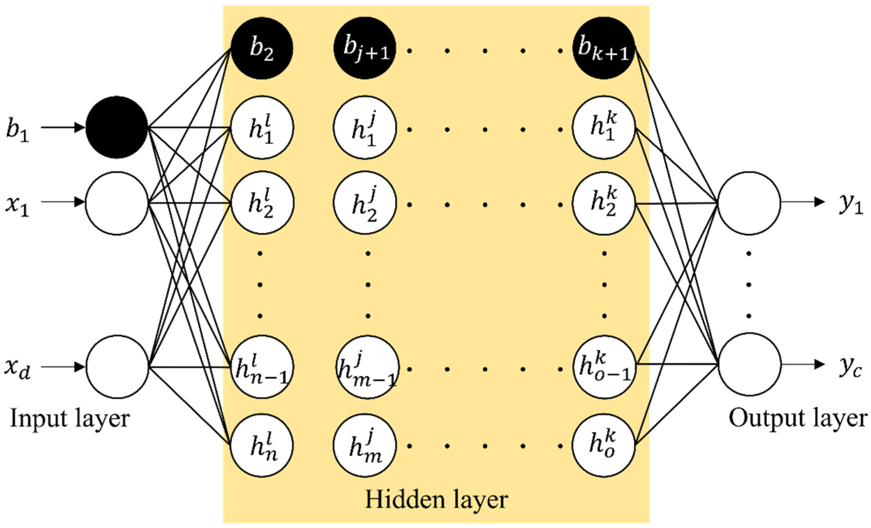
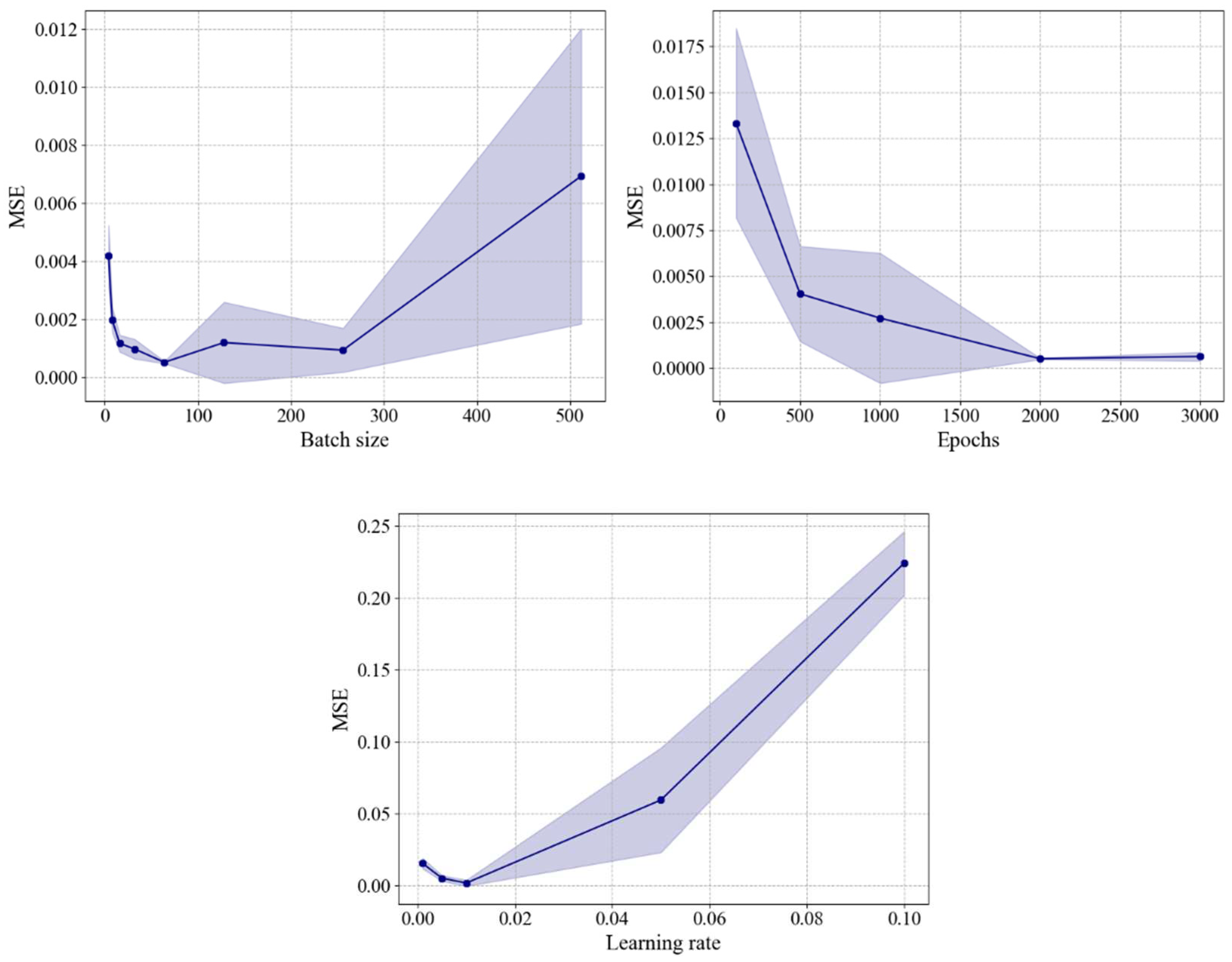
The results of the grid search cross-validation for hyperparameter optimization of the DNN model using a total of 690 source data (1,000 TEU) are presented in Figure 9. The Mean Squared Error (MSE) was used to assess the prediction accuracy for each hyperparameter. In this study, three hyperparameters were optimized, and the optimal values for each parameter are as follows; 1) batch size: [4, 8, 16, 32, 64, 128], 2) epochs: [100, 500, 1000, 2000, 3000] and 3) learning rate: [0.001, 0.005, 0.01, 0.05, 0.1].

Figure 9. Grid search results for DNN model using source dataset.

Figure 9. Grid search results for DNN model using source dataset.

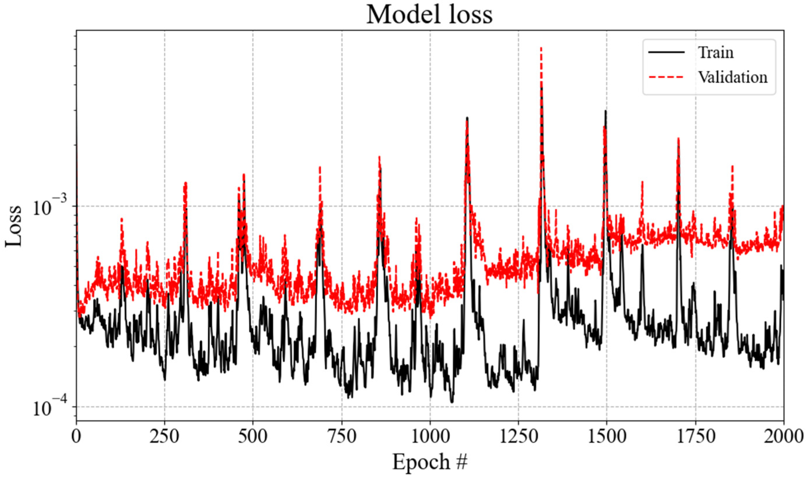
The final hyperparameters determined for the Base DNN model were chosen based on the consideration of a small mean squared error value while considering the training speed. The training hyperparameters for the base DNN model were set as follows: batch size = 64, epochs = 2000, and learning rate = 0.01. Using this combination of selected hyperparameters, the model was trained for a total of 18,000 iterations on the 1000 TEU containership dataset. The prediction accuracy of the base DNN training model is quantified by an MSE of approximately 0.0008, as shown in Figure 10. The peak of the loss typically occurs during mini-batch training with split data.

Figure 10. Loss for the base DNN models.

Figure 10. Loss for the base DNN models.

The prediction accuracy for the test dataset not used during training was evaluated to validate the learning level of the base DNN model. Table 6 presents the evaluation metrics for the test dataset of the source data, which is the 1,000 TEU containership. MSE and MAPE indicate higher prediction accuracy as their values become smaller, and an $R^2$ value closer to 1 signifies that the test dataset not used in training is being well predicted. The DNN model can accurately predict viscous resistance and wake distribution in the propeller plane, as evidenced by the high level of accuracy. 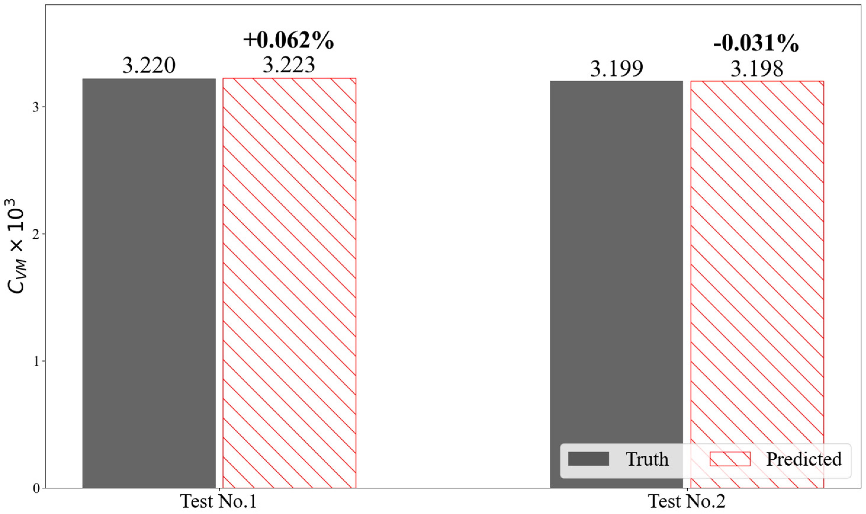Figure 11 displays the predicted viscous resistance results for the two above-mentioned test cases. The average error of the viscous resistance coefficient of model $C_{VM}$ is significantly small, being $0.00009\times {10}^{-3}$, which is less than 0.005% of the target value. 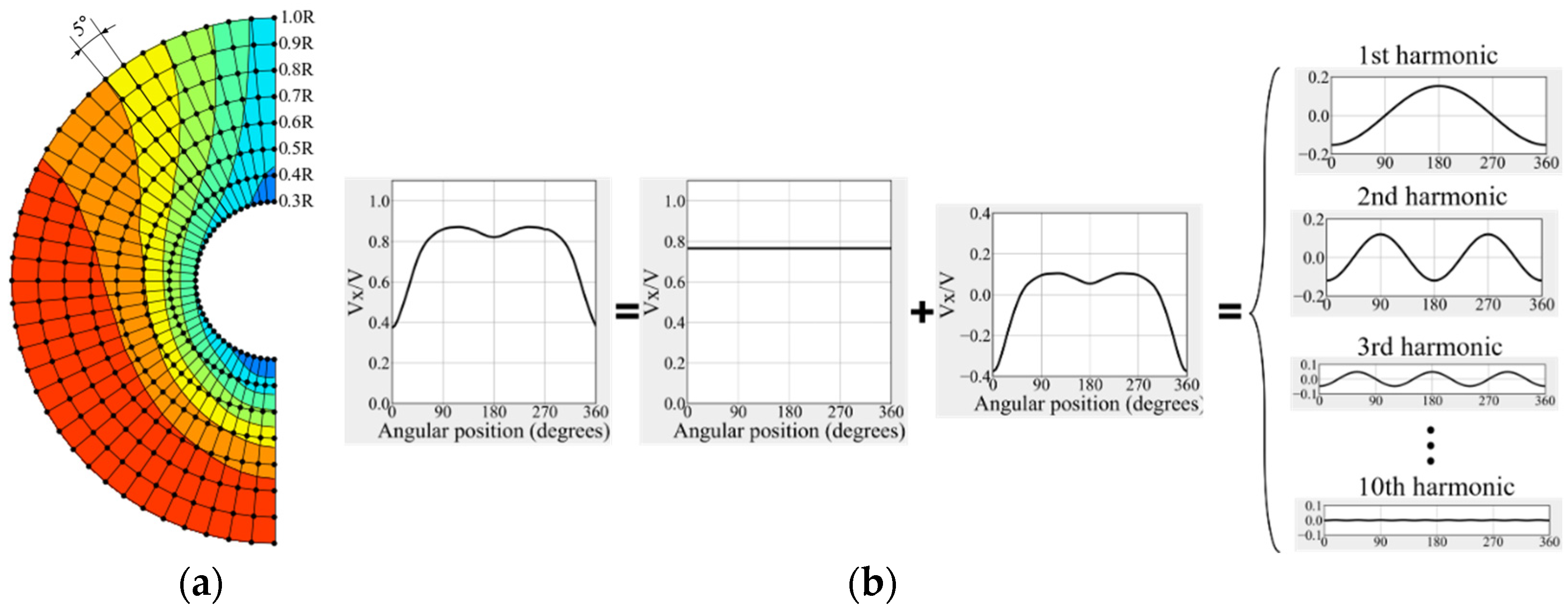Figure 12 compares the true data obtained from CFD analysis with the results predicted by the DNN. The true wake distribution is given on the left, and the predicted data is shown on the right. The true data for the circumferential distribution of the axial velocity component is depicted as black dashed lines, while the predicted data is represented by red symbols and solid lines. As observed in Figure 12, the true and predicted data closely match with high accuracy. The DNN model is capable of accurately predicting not only wake distribution but also viscosity resistance. The neural network that serves as the basis for transfer learning on a small amount of dataset requires sufficient prediction accuracy. Given the results above, it can be concluded that the base DNN model can effectively capture the design variables of the FCF and establish a strong association with both the viscous resistance coefficient and wake distribution, demonstrating high accuracy in its predictions.

Table 6. MSE, MAPE and $R^2$ values for the base DNN model

Table 6. MSE, MAPE and $R^2$ values for the base DNN model

.MSE	MAPE [%]	${\mathit{R}}^2$
0.00081	7.16	0.98

Figure 11. Evaluation of prediction accuracy by the viscous resistance coefficient for the base DNN model.

Figure 11. Evaluation of prediction accuracy by the viscous resistance coefficient for the base DNN model.

Figure 12. Evaluation of prediction accuracy by harmonic wake distribution and axial wake distribution for the base DNN model: (a) Test data no.1; (b) Test data no.2.

Figure 12. Evaluation of prediction accuracy by harmonic wake distribution and axial wake distribution for the base DNN model: (a) Test data no.1; (b) Test data no.2.

4.3. Prediction results using target dataset (DNN-TL model)

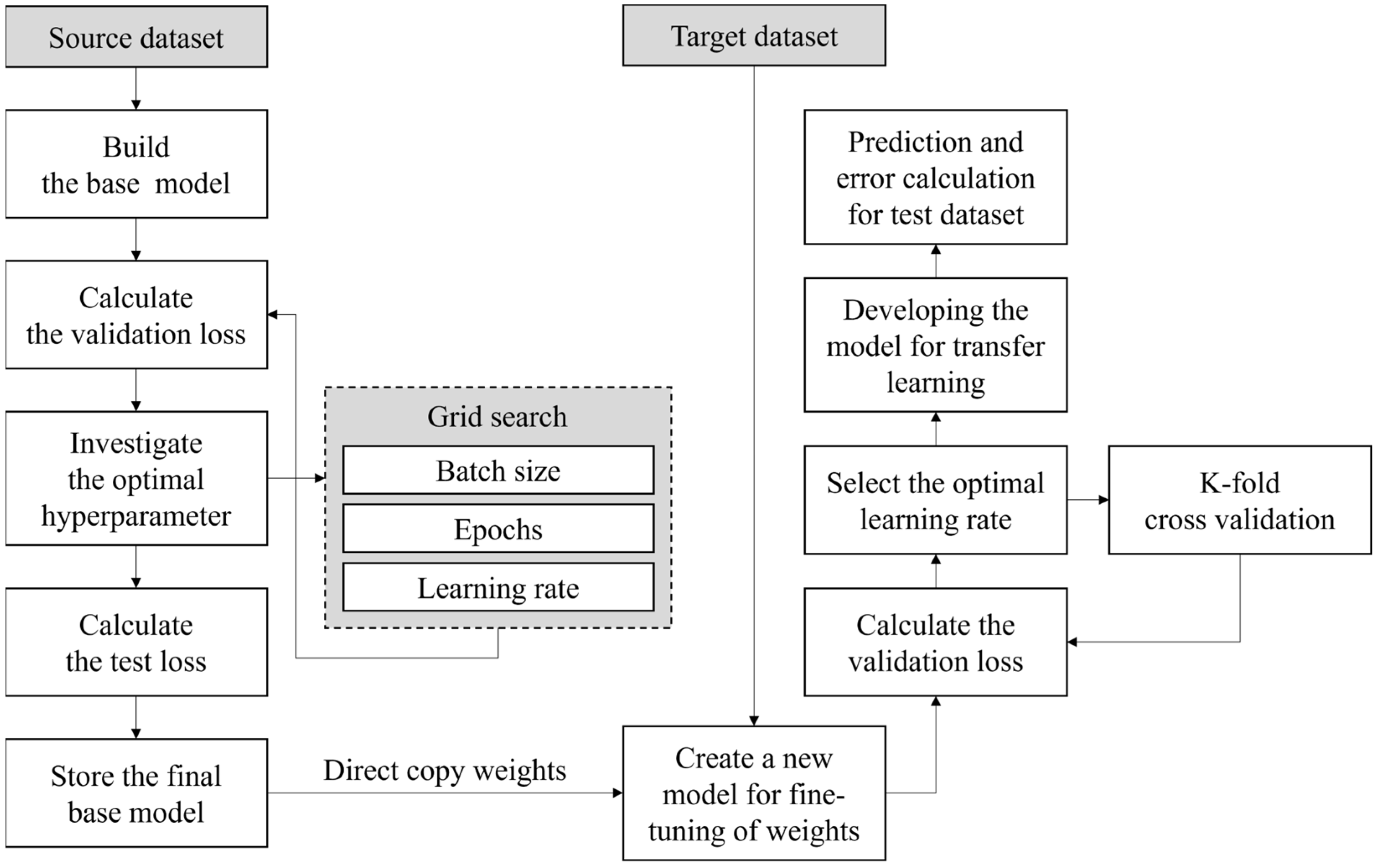
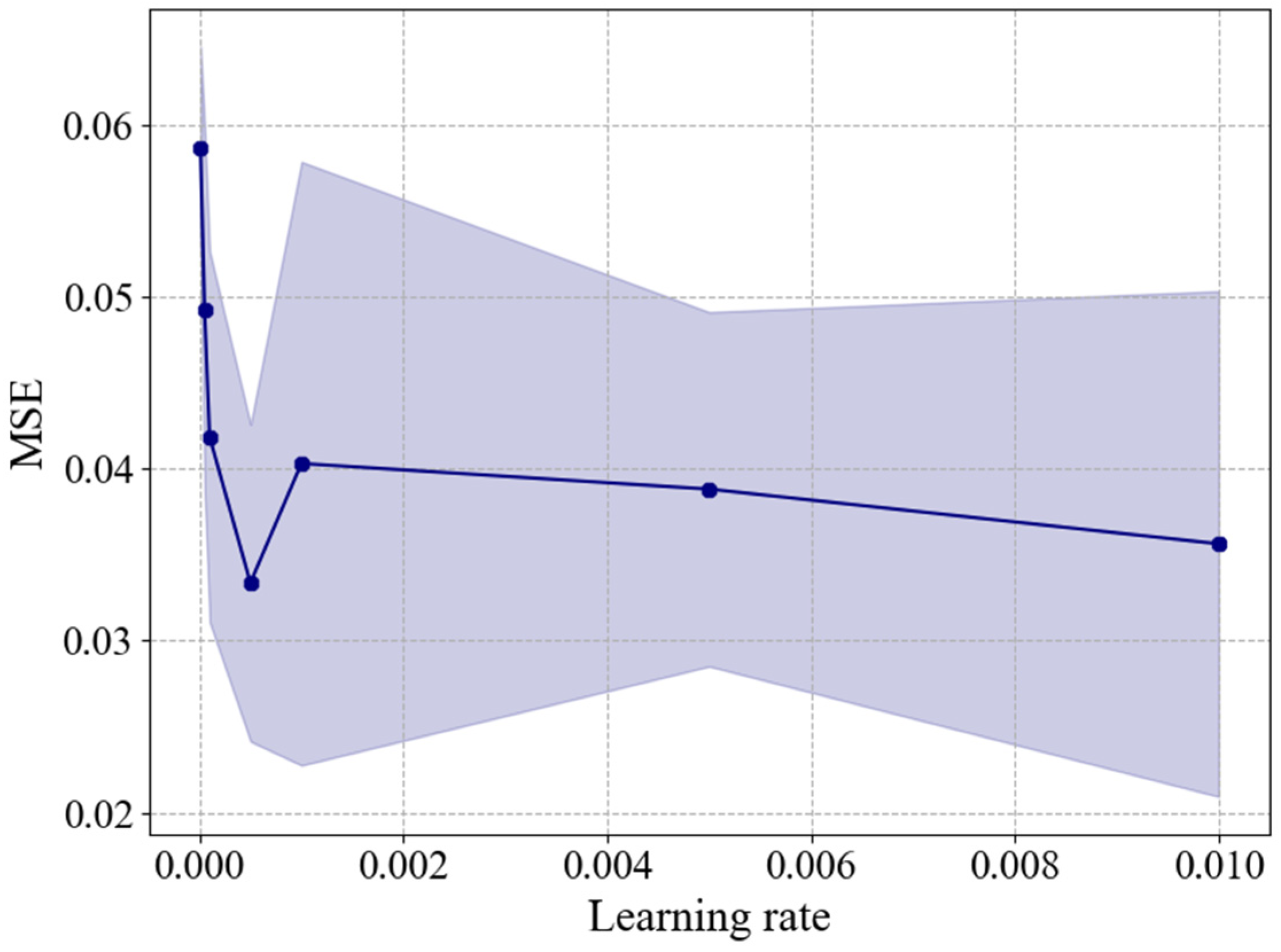
The DNN-TL model is reconstructed and retrained based on the weights of the previously trained DNN model, using only the target dataset. Since the size of the target dataset is considerably smaller (150 datasets) compared to the source dataset, a smaller learning rate is necessary to ensure training accuracy. 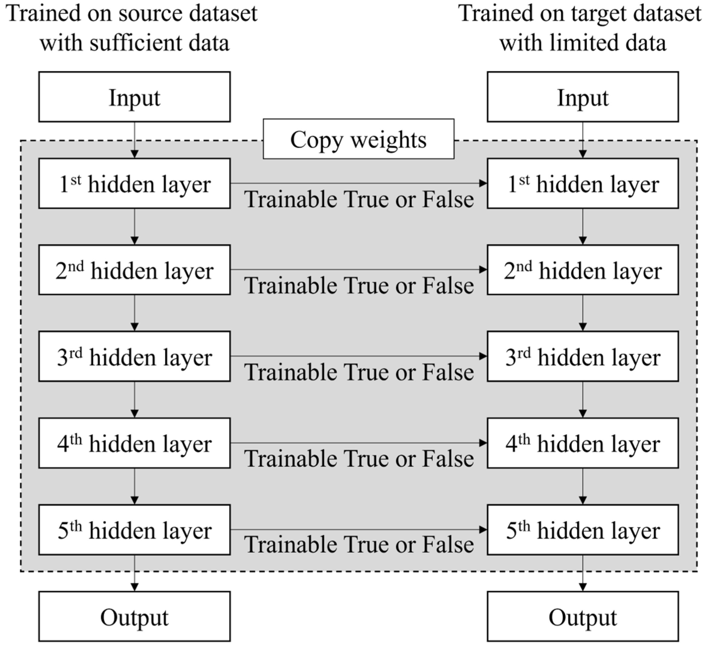Therefore, it is necessary to find the optimal learning rate value for the training dataset of the DNN-TL model The optimization was performed with learning rates [0.00001, 0.00005, 0.0001, 0.0005, 0.001, 0.005, 0.01], and the comparison of MSE values for each value is shown in Figure 13. In this study, the optimal learning rate value for predicting the viscous resistance and wake distribution of the target dataset (2,500 TEU and 3,600 TEU) is determined to be 0.0005. Based on this, the parameters of the DNN-TL model were constructed. To verify the prediction of viscous resistance and wake distribution based on transfer learning, different configurations were tested: DNN-TL models with 1, 4, and 5 fixed layers, as well as a DNN-TL model without any fixed layers (Table 7). Fine-tuning was performed on each of these configurations, and their performances were compared. In the DNN-TL model, the weights of neurons are initialized based on the previously trained base model, and the model is retrained and reconstructed using the training dataset from the target dataset.

Figure 13. Optimization of the learning rate for DNN-TL model using target dataset.

Figure 13. Optimization of the learning rate for DNN-TL model using target dataset.

Table 7. Fine-tuning for DNN-TL.

Table 7. Fine-tuning for DNN-TL.

	1st hidden layer	2nd hidden layer	3rd hidden layer	4th hidden layer	5th hidden layer
All fixed layer	Fixed	Fixed	Fixed	Fixed	Fixed
Fixed 4 layer	Fixed	Fixed	Fixed	Fixed	Train
Fixed 1 layer	Fixed	Train	Train	Train	Train
No fixed layer	Train	Train	Train	Train	Train

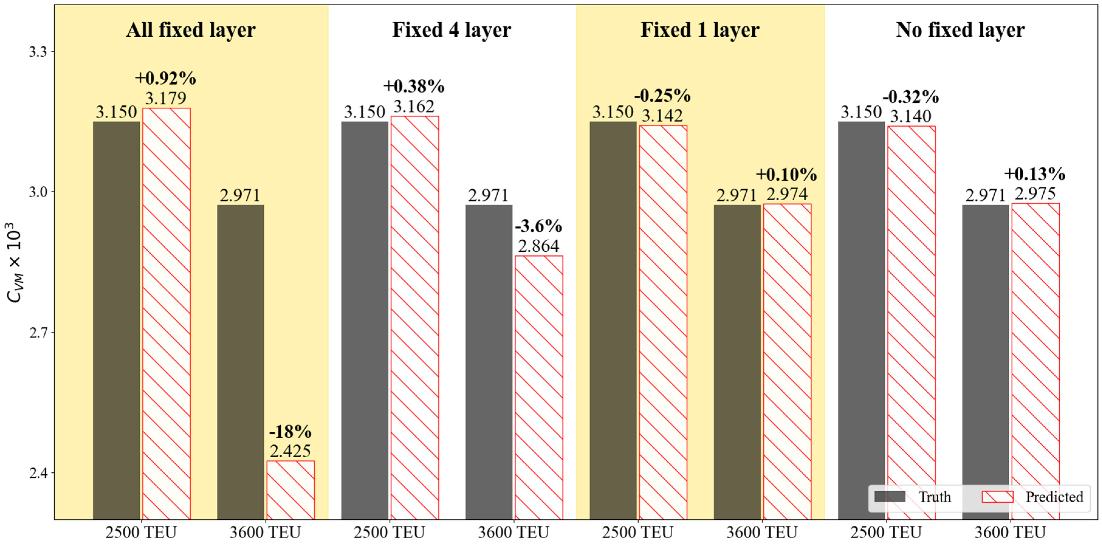
The prediction accuracy based on fine-tuning of hidden layer weights was evaluated to verify the level of learning. Figure 14 compares the predicted viscous resistance coefficients of the model ship for each fine-tuning condition. The black-filled bar chart represents the true values obtained from CFD analysis, while the red dashed-filled bars represent the predicted results from each fine-tuning condition. The viscosity resistance performance was compared using one test data for each of the 2,500 TEU and 3,600 TEU containerships. 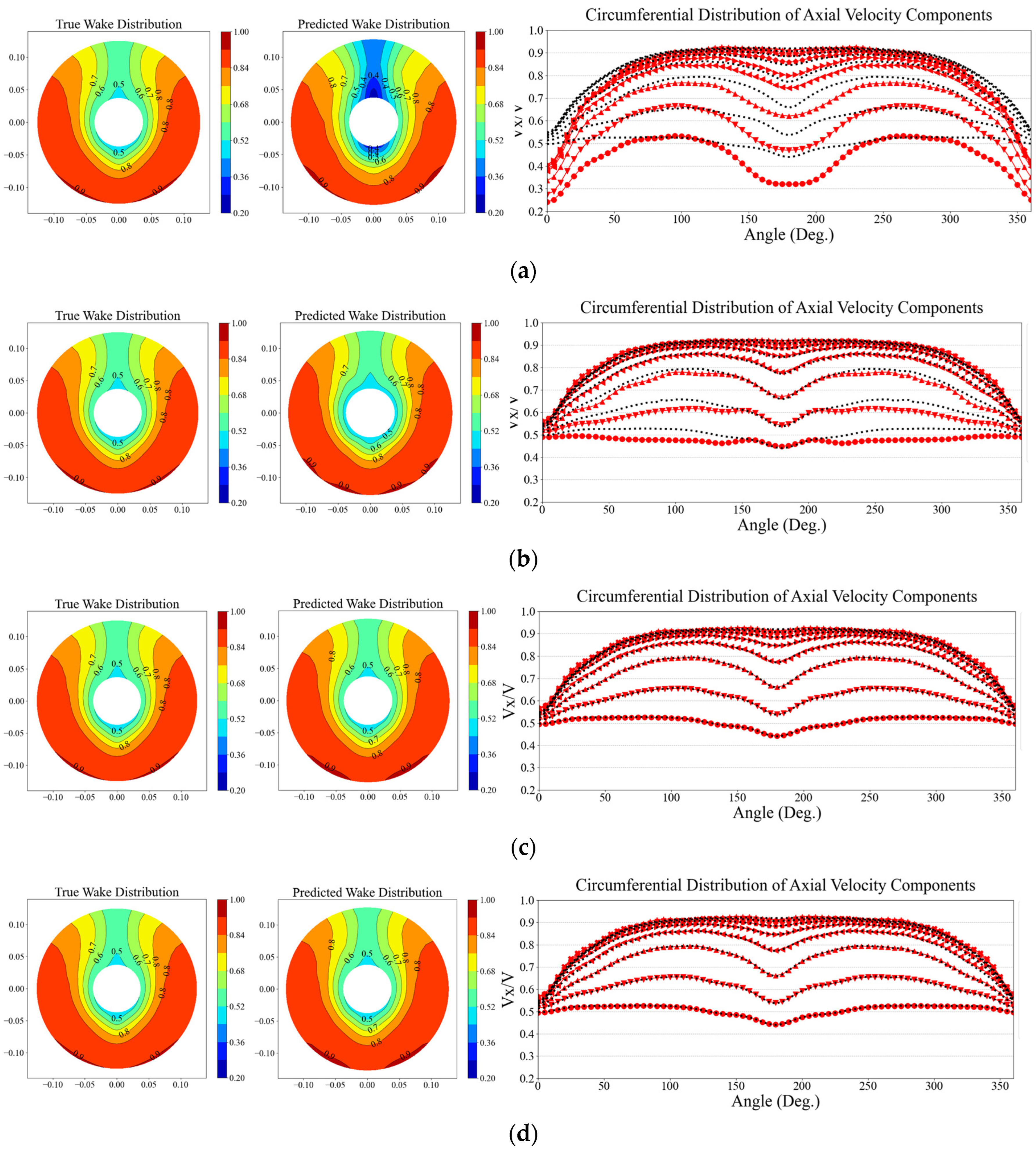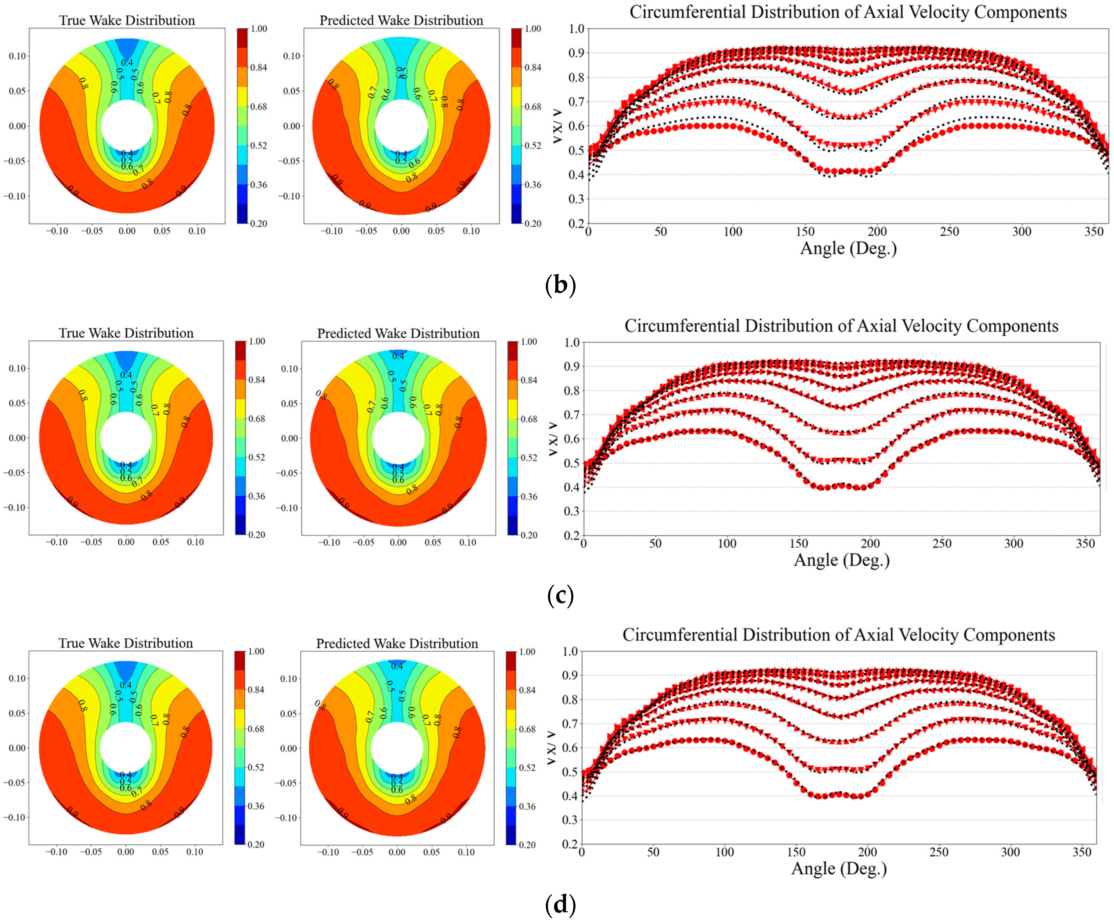Figure 15 and Figure 16 illustrate the comparison of predicted results for harmonic wake distribution and circumferential distribution of axial velocity components for both 2,500 TEU and 3,600 TEU. The left figure shows the harmonic wake distribution obtained from CFD analysis, and the middle part displays the predicted wake distribution from each fine-tuning condition. In the case where the weights of all five hidden layers are fixed (All fixed layer case), there is an error of 18% specifically in the viscosity resistance coefficient ($C_{VM}$) for the 3,600 TEU containership. The accuracy of predicting the axial velocity distribution in the propeller plane is also quite low, and it can be observed that it is trying to follow the wake distribution characteristics of the 1,000 TEU used in the base DNN model. In the case of ‘Fixed 4 layer’, where only the weights of the last layer among the layers were trained, $C_{VM}$ for 2,500 TEU and 3,600 TEU show errors of 0.38% and -3.6% respectively. This indicates an improvement in prediction accuracy compared to the ‘All fixed layer’ case. In Figure 15(b) and Figure 16(b), compared to the ‘All fixed layer’, there is an attempt to capture the characteristics of each hull-form. This indicates that the weights of the last hidden layer among the hidden layers play a role in conveying a certain level of knowledge about the target datasets (2,500 TEU and 3,600 TEU). The prediction results for the Fixed 1 layer, where only the weights of the first hidden layer are not retrained, and the No fixed layer, where all layers are retrained, show a quite similar trend. The $C_{VM}$ prediction results for both 2,500 TEU and 3,600 TEU exhibit errors within 0.5%. When observing the wake distribution and axial velocity components figures, it is evident that the characteristics of each linear component are sufficiently captured.

Figure 14. Evaluation of prediction accuracy by the viscous resistance coefficient for the target dataset (2,500 TEU and 3,600 TEU) between each fine-tuning condition.

Figure 14. Evaluation of prediction accuracy by the viscous resistance coefficient for the target dataset (2,500 TEU and 3,600 TEU) between each fine-tuning condition.

Figure 15. Evaluation of prediction accuracy by harmonic wake distribution and axial wake distribution for 2,500 TEU between each fine-tuning condition: (a) All fixed; (b) Fixed 4 layer; (c) Fixed 1 layer; (d) No fixed layer.

Figure 15. Evaluation of prediction accuracy by harmonic wake distribution and axial wake distribution for 2,500 TEU between each fine-tuning condition: (a) All fixed; (b) Fixed 4 layer; (c) Fixed 1 layer; (d) No fixed layer.

Figure 16. Evaluation of prediction accuracy by harmonic wake distribution and axial wake distribution for 3,600 TEU between each fine-tuning condition: (a) All fixed; (b) Fixed 4 layer; (c) Fixed 1 layer; (d) No fixed layer.

Figure 16. Evaluation of prediction accuracy by harmonic wake distribution and axial wake distribution for 3,600 TEU between each fine-tuning condition: (a) All fixed; (b) Fixed 4 layer; (c) Fixed 1 layer; (d) No fixed layer.

Table 8 presents the prediction accuracy metrics for the test dataset that was not used in the training process under each fine-tuning condition. MSE and MAPE are metrics where lower values indicate higher accuracy in predictions. $R^2$, on the other hand, is a measure of how well the model explains the variance in the data. A higher $R^2$ value, closer to 1, indicates a better predictive performance. Generally, when $R^2>0.67$, it is considered to have a reasonably good predictive accuracy, while $0.33<R^2<0.67$ indicates moderate predictive performance, and $0.16<R^2<0.32$ suggests poor predictive performance [16]. The $R^2$ score for the ‘All fixed layer’ case is -4.163, indicating no prediction capability on the test dataset. Conversely, when the first hidden layer is fixed, it exhibits the highest scores across all accuracy metrics. It is considered that the weights of the first layer in the previously trained base DNN model were tailored to capture the characteristics of the viscous resistance coefficient on containership and the axial velocity on the propeller plane. The remaining hidden layers seem to have been designed to understand the fluid characteristics by hull-form. To assess the level of prediction accuracy in this study, the performance was compared to accuracy metrics from other literature that used transfer learning for predictions. Solis and Calvo-Valverde [17] applied DNN and TL to time series prediction, and their optimal prediction model achieved a MAPE value of approximately 9%. Zhou et al. [18] predicted the dynamic behavior of a gas turbine engine using transfer learning, and in their optimal prediction model, they achieved MSE and $R^2$ values of 0.00466 and 0.881, respectively. The MSE, MAPE, and $R^2$ values in this paper all fall within a similar range, indicating that the prediction model applied with transfer learning is at a satisfactory level of accuracy.

Table 8. MSE, MAPE and $R^2$ values for each fine-tuning conditions

Table 8. MSE, MAPE and $R^2$ values for each fine-tuning conditions

.	MSE	MAPE [%]	${\mathit{R}}^2$
All fixed layer	0.3083	182.4	-4.163
Fixed 4 layer	0.0307	24.88	0.499
Fixed 1 layer	0.0086	13.89	0.854
No fixed layer	0.0185	18.40	0.703

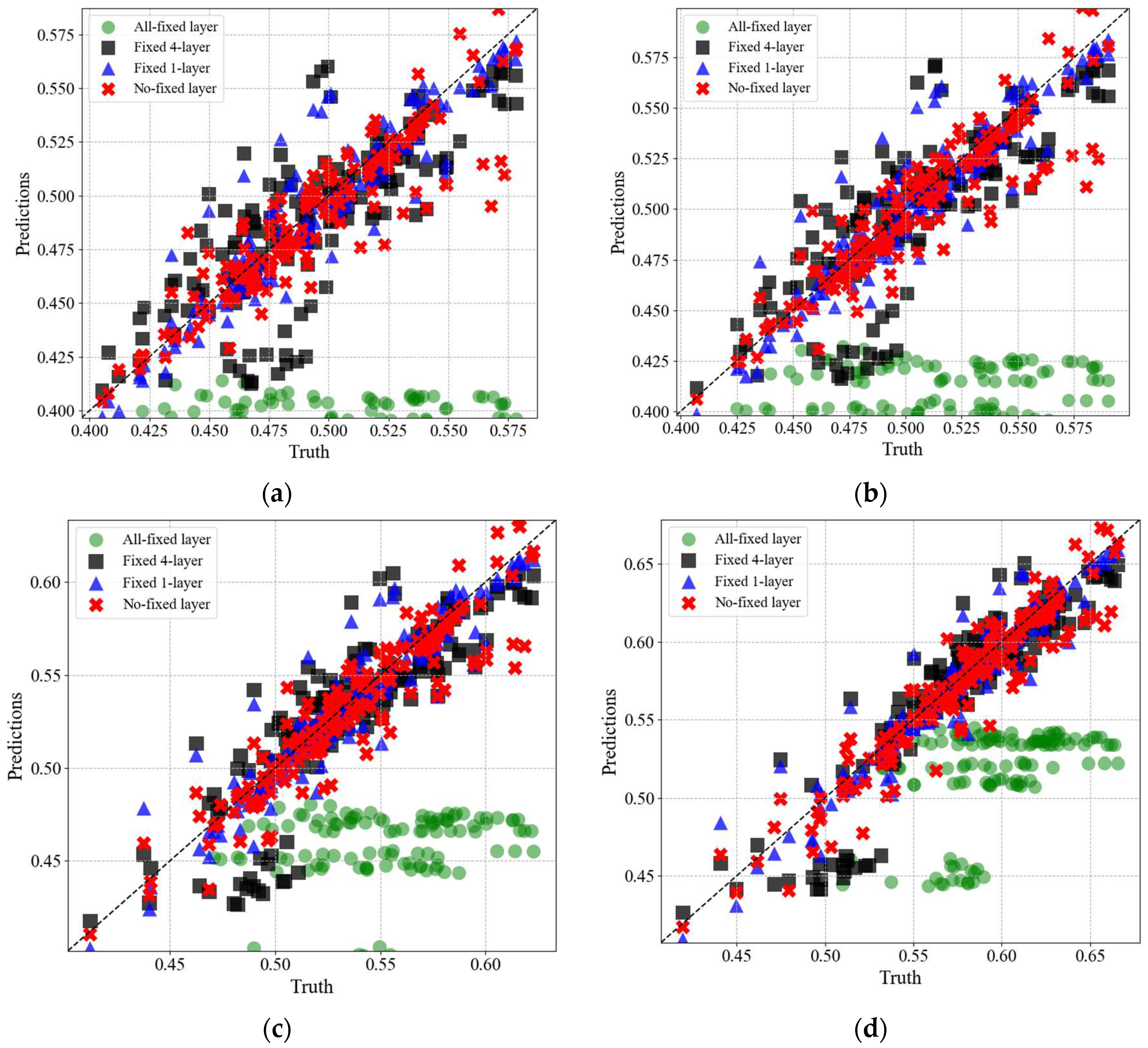
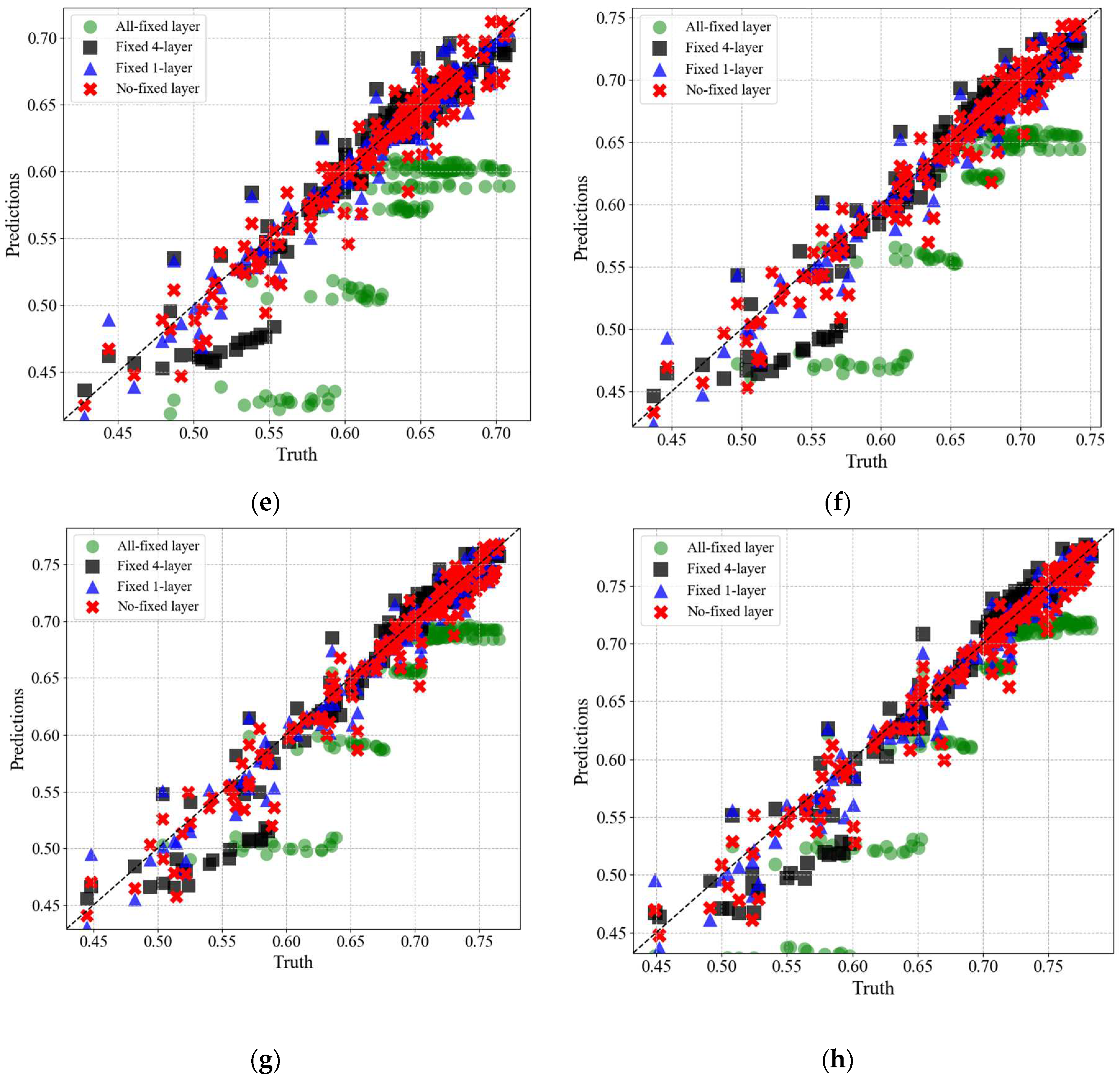
Figure 17 compares the predicted radial profiles of axial velocity components from the four tuning cases with their true values. The green circles represent the predictions from the ‘All fixed layer’ condition, the black squares are from the case where the first four layers were fixed (Fixed 4 layer), the blue triangles represent the condition where only the first layer was fixed (Fixed 1 layer), and the red ‘X’ symbols depict the predictions from the ‘No fixed layer’ condition. In the case of ‘All fixed layer’, significant discrepancies are observed between the predicted values and the true values across all radii. On the other hand, for the ‘Fixed 1 layer’ and ‘No fixed layer’ cases, it can be observed that the predicted values closely follow the trends of the true values.

Figure 17. Predictions for the circumferential distribution of axial velocity components for each radius: (a) R=0.30; (b) R=0.40; (c) R=0.50; (d) R=0.60; (e) R=0.70; (f) R=0.80; (g) R=0.90; (h) R=1.00.

Figure 17. Predictions for the circumferential distribution of axial velocity components for each radius: (a) R=0.30; (b) R=0.40; (c) R=0.50; (d) R=0.60; (e) R=0.70; (f) R=0.80; (g) R=0.90; (h) R=1.00.

5. Conclusions

References

1. Samsung Heavy Industry (2007), Flow control appendages for improvement of pressure resistance and hull vibration, Korean patent 0 B 1007.
2. Lee, H. D.; Hong, C. B.; Kim, H. T.; Choi, S. H.; Han, J. M.; Kim, B.; Lee, J. H. Development and application of energy saving devices to improve resistance and propulsion performance. The Twenty-fifth International Ocean and Polar Engineering Conference, Kona, Big Island, Hawaii, USA, 21-26 June 201. 26 June.
3. Kim, D. J.; Oh, W. J.; Park, J. W.; Jeong, S. M. A Study on Flow Characteristics due to Dimension Variations of the Vertical Plate for Controlling the Ship Stern Flow. Journal of the Korean Society of Marine Environment & Safety 2016, 22(5), 576–582. [Google Scholar]
4. Lee, J.; Kim, I.; Park, D. W. A Study on the Resistance Performance and Flow Characteristic of Ship with a Fin Attached on Stern Hull. Journal of the Korean Society of Marine Environment & Safety 2021, 27(7), 1106–1115. [Google Scholar]
5. Park, Y.; Hwangbo, S. M.; Yu, J-W.; Cho, Y.; Lee, J. H.; Lee, I. Development of a small-sized tanker with reduced greenhouse gas emission under in-service condition based on CFD simulation. Ocean Engineering 2022, 286, 115588.
6. Hwangbo, S.; Shin, H. Statistical prediction of wake fields on propeller plane by neural network using back-propagation. Journal of Ship and Ocean Technology 2000, 4(3), 1–12. [Google Scholar]
7. Kim, S.-Y.; Moon, B. Wake distribution prediction on the propeller plane in ship design using artificial intelligence. Ships and Offshore Structures 2006, 1(2), 89–98. [Google Scholar] [CrossRef]
8. Wie, D.-E.; Kim, D.-J. The Design Optimization of a Flow Control Fin Using CFD. Journal of the Society of Naval Architects of Korea 2012, 49(2), 174–181. [Google Scholar] [CrossRef]
9. Lee, M-K. ; Lee, I. Optimal Design of Flow Control Fins for a Small Container Ship Based on Machine Learning. Journal of Marine Science and Engineering 2023, 11(6), 1149. [Google Scholar] [CrossRef]
10. Kim, J. H.; Choi, J. E.; Choi, B. J.; Chung, S. H.; Seo, H. W. Development of energy-saving devices for a full slow-speed ship through improving propulsion performance. International Journal of Naval Architecture and Ocean Engineering 2015, 7(2), 390–398. [Google Scholar] [CrossRef]
11. ITTC. Uncertainty Analysis in CFD, Verification and Validation Methodology and Procedures, Recommended Procedures and Guidelines. International Towing Tank Conference 2017, 7.5-03-01-01, 4–8.
12. Qiao, J.; Liu, X.; Chen, Z. Prediction of the remaining useful life of lithium-ion batteries based on empirical mode decomposition and deep neural networks. IEEE Access 2020, 8, 42760–42767. [Google Scholar] [CrossRef]
13. Babaeiyazdi, I.; Rezaei-Zare, A.; Shokrzadeh, S. Transfer Learning With Deep Neural Network for Capacity Prediction of Li-Ion Batteries Using EIS Measurement. IEEE Transactions on Transportation Electrification 2022, 9(1), 886–895. [Google Scholar] [CrossRef]
14. Shen, S.; Sadoughi, M.; Li, M.; Wang, Z.; Hu, C. Deep convolutional neural networks with ensemble learning and transfer learning for capacity estimation of lithium-ion batteries. Applied Energy 2020, 260, 114296. [Google Scholar] [CrossRef]
15. Park, K. M. Machine classification in ship engine rooms using transfer learning. Journal of the Korean Society of Marine Environment & Safety 2021, 27(2), 363–368. [Google Scholar]
16. Chin, W. W.; Marcolin, B. L.; Newsted, P. R. A partial least squares latent variable modeling approach for measuring interaction effects: Results from a Monte Carlo simulation study and an electronic-mail emotion/adoption study. Information systems research 2003, 14(2), 189–217. [Google Scholar] [CrossRef]
17. Solís, M.; Calvo-Valverde, L. A. A. Performance of Deep Learning models with transfer learning for multiple-step-ahead forecasts in monthly time series. arXiv preprint arXiv:2203.11196 2022. arXiv:2203.11196 2022.
18. Zhou, D.; Hao, J.; Huang, D.; Jia, X.; Zhang, H. Dynamic simulation of gas turbines via feature similarity-based transfer learning. Frontiers in Energy 2020, 14, 817–835. [Google Scholar] [CrossRef]