Modeling the Interaction of the Rolling Stock and the Track in the Emergency Braking Mode of a Passenger Train

Preprint

Article

Modeling the Interaction of the Rolling Stock and the Track in the Emergency Braking Mode of a Passenger Train

This version is not peer-reviewed.

Altmetrics

Downloads

125

Views

Comments

Submitted:

09 September 2023

Posted:

13 September 2023

You are already at the latest version

Abstract

The article analyzes the transitional mode of movement of a passenger train caused by emergency braking by the driver. To study the possibility of derailment of passenger cars, a simulation model of the movement of a train consisting of a locomotive and twenty passenger cars was developed in the Universal Mechanism software environment, designed to study the dynamics and kinematics of mechanical systems, which include railway rolling stock. The developed model allows taking into account the longitudinal, transverse and vertical vibrations of all cars and locomotive. All bodies in the model are assumed to be absolutely rigid. The assumption of non-deformability of the bodies is based on the fact that the stiffness of the spring suspension and elastic connections is significantly less than the structural rigidity of the bogie frames and the bolster structure, and the frequency of elastic vibrations of these bodies is much higher than the frequency of their vibrations on the spring suspension. Passengers and cargo in a wagon are considered to be non-deformable and integral with the wagon body, similarly in the case of a locomotive body. Between the elements of the system, connections are involved that regulate certain relative movements of these elements.

Keywords:

Subject:

Engineering - Transportation Science and Technology

1. Introduction

Rail transport and its infrastructure can cause increased danger to people, animals and other objects. In the event of an emergency situation caused by the appearance of people, animals on the railway track or the presence of other reasons that prevent the movement of the train [1], the driver is obliged to stop the movement, including by applying the emergency braking mode [2].

According to the normative and technical documentation, the use of emergency braking is permissible for the following reasons:

− unsatisfactory operation or failure of the automatic brakes of the rolling stock;
− impossibility of the train to stop after service braking;
− the appearance of animals or people on the tracks;
− threat to the safety of people's lives;
− a threat to traffic safety.

To date, a number of methods have been developed to refine brake calculations, but most of them are based on significant assumptions and do not take into account many significant factors [3]. These methods were developed at a time when the performance of computing systems lagged behind the modern level by 3-4 orders of magnitude (meaning some average estimate, including not only speed, but also the very possibility of implementing certain technologies that require significant amounts of RAM). The current capabilities make it possible to use much more accurate information (characteristics of dependencies, data structures and algorithms) in modeling processes, as well as to perform resource-intensive optimization calculations. At the moment, the problem of interaction between the rolling stock and the railway track has been studied quite fully [4]. In the works of various researchers [5], the possibility of rationalizing the braking technology by using multi-stage braking, depending on the parameters of the composition, profile, track plan and other conditions, without loss of braking efficiency is already quite formally proved [6]. Thus, in these works, the prerequisites for the application of optimization technologies to the rolling stock braking process are laid. However, at present, there are practically no works on the study of the braking of passenger and freight trains in an emergency mode, including using the methods of mathematical and simulation modeling [7]. To simulate the emergency braking of a passenger train, mathematical (computer) models of a locomotive and a wagon were compiled and an analysis was made of their interaction with each other and the railway track [8].

2. Materials and Methods

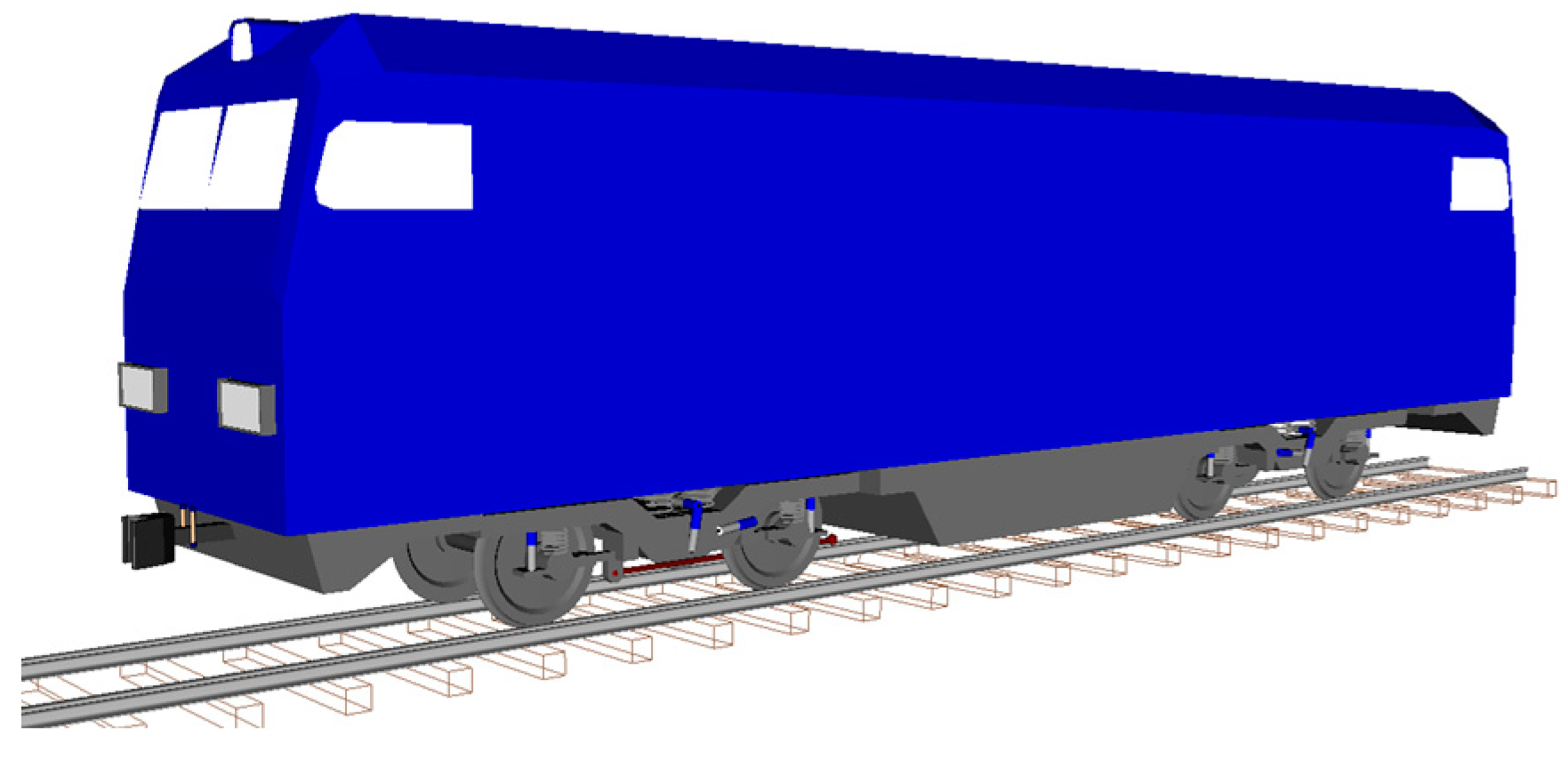
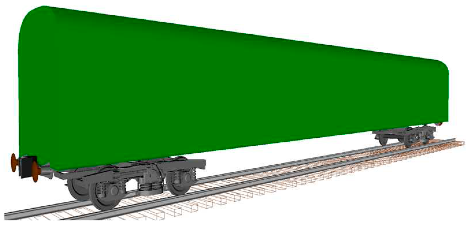
The locomotive model includes a body, 2 bogie frames (including the weight of 4 traction motors), 2 automatic couplers, 2 thrust plates and 4 wheelsets with axle boxes (see Figure 1). It should be noted here that in order to speed up the calculation time, the locomotive model does not take into account the power elements and bodies responsible for traction [9]. The passenger car model consists of a body, 2 bogie pivot beams, 2 bogie frames, 4 bogie cradles, 2 automatic couplers, 2 thrust plates, 4 buffers and 4 wheelsets with axle boxes (see Figure 2). The considered mathematical description of the calculation of the kinematic characteristics of the bodies of the system is implemented in the "Universal Mechanism" complex in the form of a software procedure for specifying a hinge connecting the body under consideration with the base coordinate system (CS). At the preliminary stage, the spatial orientation of the own coordinate system of each body included in the car model, parallel to the axes CS₀, is set. In the process of describing the hinges for each body, the vector r_i⁽⁰⁾ is specified in the initial position (at t = 0) and the type of orientation angles is chosen [10].

The equations describing the motion of the i-th body of the mechanical system "car-track" when SCi coincides with the main axes of inertia of the bodies have the form:

\{\begin{matrix} m_{i} \cdot a_{i x}^{(0)} = \sum F_{i x}^{(0)} + \sum R_{i x}^{(0)} \\ m_{i} \cdot a_{i y}^{(0)} = \sum F_{i y}^{(0)} + \sum R_{i y}^{(0)} \\ m_{i} \cdot a_{i z}^{(0)} = \sum F_{i z}^{(0)} + \sum R_{i z}^{(0)} \\ J_{i x}^{(i)} \cdot \frac{d ω_{i x}^{(i)}}{d t} + ω_{i y}^{(i)} ω_{i z}^{(i)} \cdot (J_{i z}^{(i)} - J_{i y}^{(i)}) = \sum M_{i x}^{(i)} + \sum L_{i x}^{(i)} \\ J_{i y}^{(i)} \cdot \frac{d ω_{i y}^{(i)}}{d t} + ω_{i z}^{(i)} ω_{i x}^{(i)} \cdot (J_{i x}^{(i)} - J_{i z}^{(i)}) = \sum M_{i y}^{(i)} + \sum L_{i y}^{(i)} \\ J_{i z}^{(i)} \cdot \frac{d ω_{i z}^{(i)}}{d t} + ω_{i x}^{(i)} ω_{i y}^{(i)} \cdot (J_{i y}^{(i)} - J_{i x}^{(i)}) = \sum M_{i z}^{(i)} + \sum L_{i z}^{(i)} \end{matrix}

(1)

where m_i – is the mass of the i-th body, kg;

a_{i x}^{(0)}

a_{i y}^{(0)}

a_{i z}^{(0)}

- is the projections of the acceleration vector of the i-th body on the coordinate axes SC₀, m/s²;

\sum F_{i x}^{(0)}

\sum F_{i y}^{(0)}

\sum F_{i z}^{(0)}

– is the sum of the projections of all active forces applied to the i-th body onto the coordinate axes SC₀, N;

\sum R_{i x}^{(0)}

\sum R_{i y}^{(0)}

\sum R_{i z}^{(0)}

– is the sum of the projections of all reactive forces applied to the i-th body onto the coordinate axes SC₀, N;

J_{i x}^{(i)}

J_{i y}^{(i)}

J_{i z}^{(i)}

– is the moments of inertia of the i-th body about the axes SC_i, kg·m²;

ω_{i x}^{(i)}

ω_{i y}^{(i)}

ω_{i z}^{(i)}

– is the projections of the angular velocity vector of the i-th body on the coordinate axes SC_i, rad/s;

\sum M_{i x}^{(i)}

\sum M_{i y}^{(i)}

\sum M_{i z}^{(i)}

– is the sum of the moments of all active forces applied to the i-th body relative to the axes SC_i, N/m;

\sum L_{i x}^{(i)}

\sum L_{i y}^{(i)}

\sum L_{i z}^{(i)}

– is the sum of the moments of all reactive forces applied to the i-th body, relative to the axes SC_i, N/m.

Equations included in the system Eq. (1) are written in different coordinate systems: the first three - in the base mobile, the last three - in their own, associated with the body [11]. Based on the systems of equations (1) written for all bodies of the mechanical system, a system of second-order ordinary differential equations is determined that describes the motion of the system in generalized coordinates, with nonlinear right-hand sides (in matrix form):

M (q) \cdot {\ddot{q}}_{i} + k (q, \dot{q}) = Q

(2)

where М(q) – is the mass matrix;

k (q, \dot{q})

– is the column vector of generalized inertial forces; Q – is the column vector of generalized active forces.

The solution of the system of equations (2), with respect to generalized coordinates, allows you to determine the linear and angular displacements, velocities and accelerations of the bodies included in the car model, as well as any points belonging to the bodies, when specifying their position in the coordinate system of the corresponding body [12]. To compose equations (2), it is necessary to obtain analytical dependences of the reaction forces in the bonds between individual bodies. Power elements in the car and locomotive models include: contact interactions between bodies, elastic (spring suspension springs) and elastic-dissipative (dampers) forces.

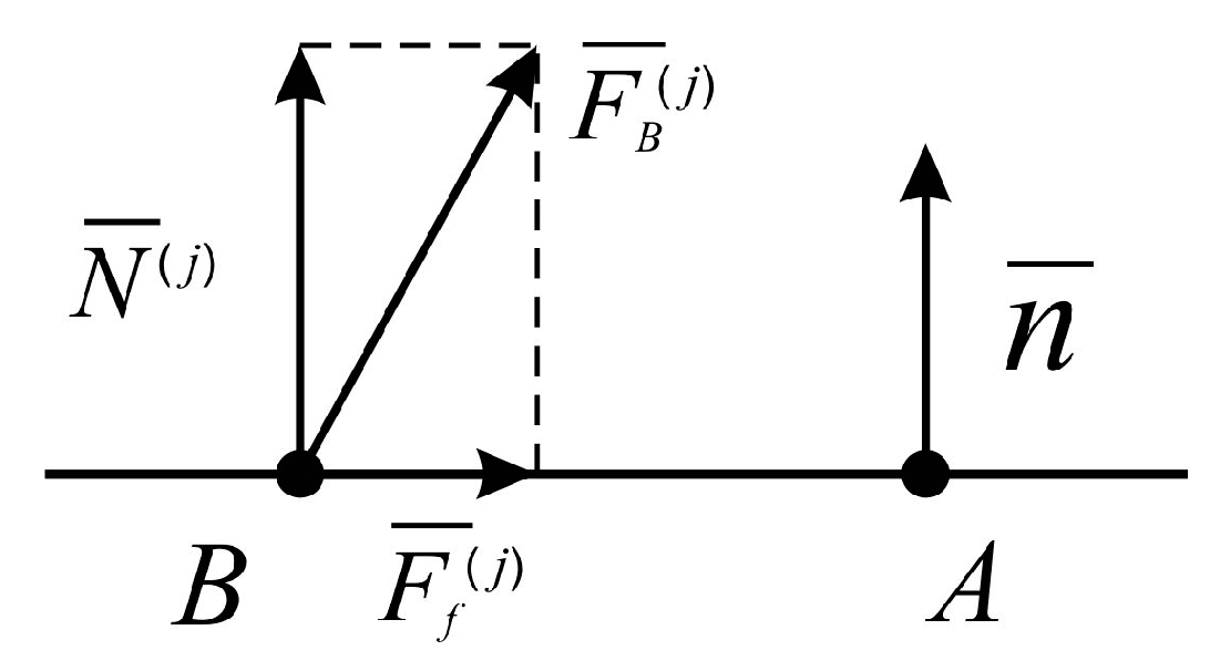
Contact interaction is used in models to simulate the interaction of side bearings, center plate-thrust center-pivot, and coupler-plate and coupler-auto coupler [13]. When describing the contact interaction of bodies, it is assumed that an infinite plane is associated with one of the contacting bodies, and a set of contact points is associated with the second body. With a positive value of Δ, there is no contact between the bodies, and with a negative value, the contact force acting from the first body to the second is described by the following mathematical model in vector form (see Figure 3):

{\bar{F}}_{B}^{(j)} = \{\begin{cases} 0, Δ \geq 0 \\ {\bar{N}}_{}^{(j)} + {\bar{F}}_{f}^{(j)}, Δ < 0 \end{cases}

(3)

where N – is the normal reaction vector; F_f – is the friction force vector.

The normal reaction is described by a linear elastic-dissipative model and is determined in SC_j from the expression:

N^{(j)} = - Δ \cdot C_{B} - \frac{d Δ}{d t} β_{B}

(4)

where С_В – is the contact stiffness coefficient at point B; β_В – is the contact dissipation coefficient at point B.

For the Coulomb friction force, there are two regimes: sliding and adhesion [14]. In the sliding mode, a mathematical model of force is implemented, which is described by the following expression:

F_{f}^{(j)} = \frac{- f N^{(j)} \cdot ν_{S}^{j}}{|ν_{S}^{(j)}|}

(5)

where f – is the sliding friction coefficient; ν_S – is the sliding speed of one body.

The transition to the clutch friction mode is carried out at the moment when the relative motion of one body relative to another stop, i.e. when the relative slip velocity vector ν_S changes its direction. In this mode, the clutch friction force is determined by the expression:

F_{f}^{(j)} = - f_{0} \cdot N^{(j)}

(6)

where f₀ – is the clutch friction coefficient.

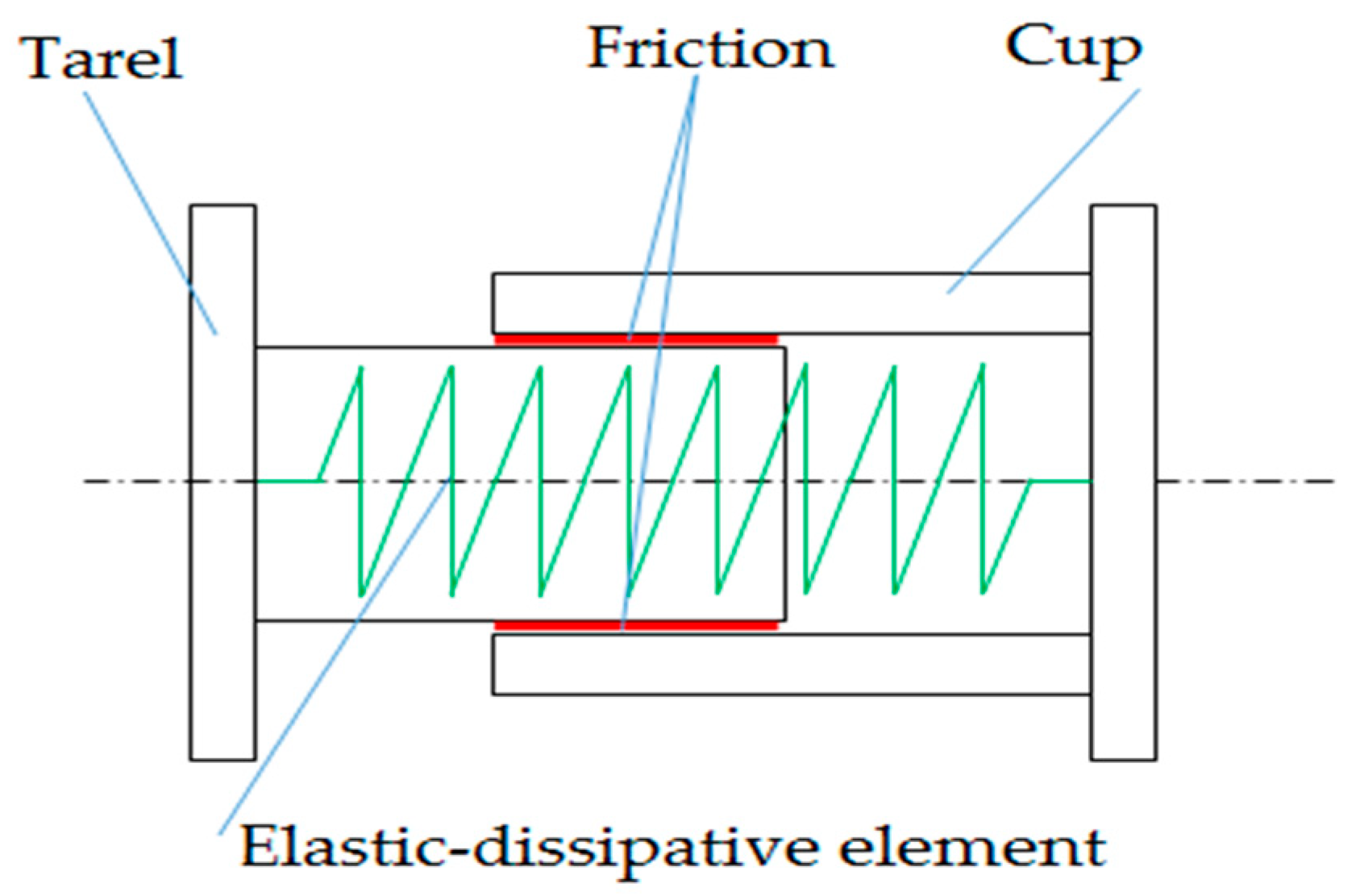
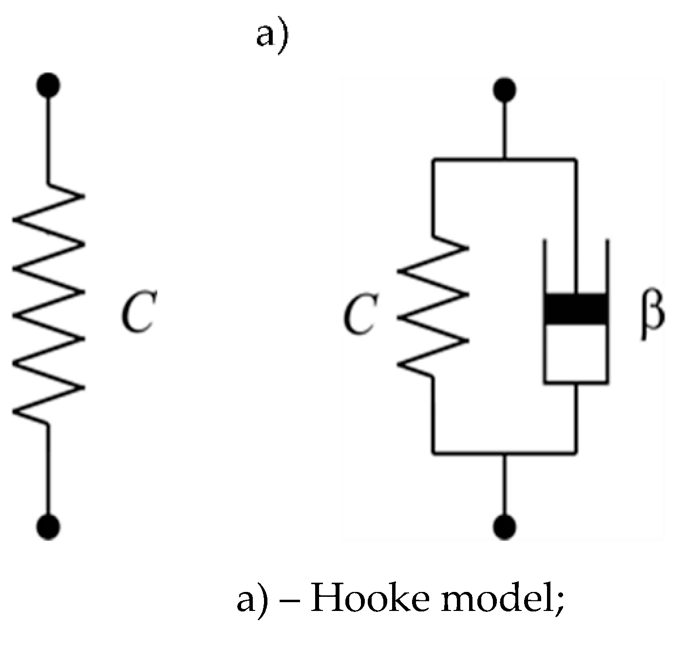
Springs, dampers, rods and other connections are implemented using elastic and elastic-viscous power elements. In this paper, the rheological models of Hooke and Voigt [15], respectively, are used to describe elastic and elastic-viscous force elements (see Figure 4).

The mathematical model of force F and moment M in the coordinate system of the elastic element are determined by the following expression in matrix form:

F = C_{r} \cdot d R_{B}^{(A)}

(7)

M = C_{ϕ} \cdot d A_{B}^{(A)}

(8)

where С_r – is the linear stiffness matrix; C_ϕ – is the angular stiffness matrix;

d R_{B}^{(A)}

– is the matrix of linear deformation of the elastic element;

d A_{B}^{(A)}

– is the matrix of direction cosines of the angular deformation of the element.

Mathematical models of force F_D and moment M_D of an elastic-dissipative element are determined by the following expressions in matrix form:

F_{D} = C_{r} \cdot d R_{B}^{(A)} + D_{r} \cdot d {\dot{R}}_{B}^{(A)}

M_{D} = C_{ϕ} \cdot d A_{B}^{(A)} + D_{ϕ} \cdot d {\dot{A}}_{B}^{A}

(9)

where D_r – is the linear dissipation matrix; D_ϕ – is the angular dissipation matrix.

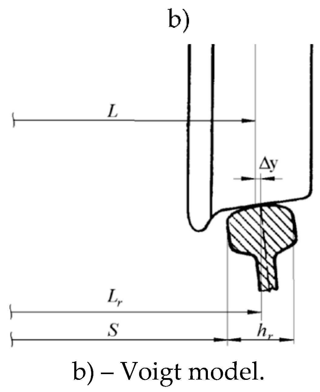
The position of the rail in the transverse direction in an ideal straight line is set by the gauge widening parameter Δy in a straight line (see Figure 5).

Δ y = \frac{L_{r} - L}{2}

(10)

Δ y = \frac{S + h_{r} - L}{2}

(11)

where L_r – is the distance between the centers of the rail heads; L – is the distance between wheelset laps; S – is the track gauge; h_r – is the rail head width.

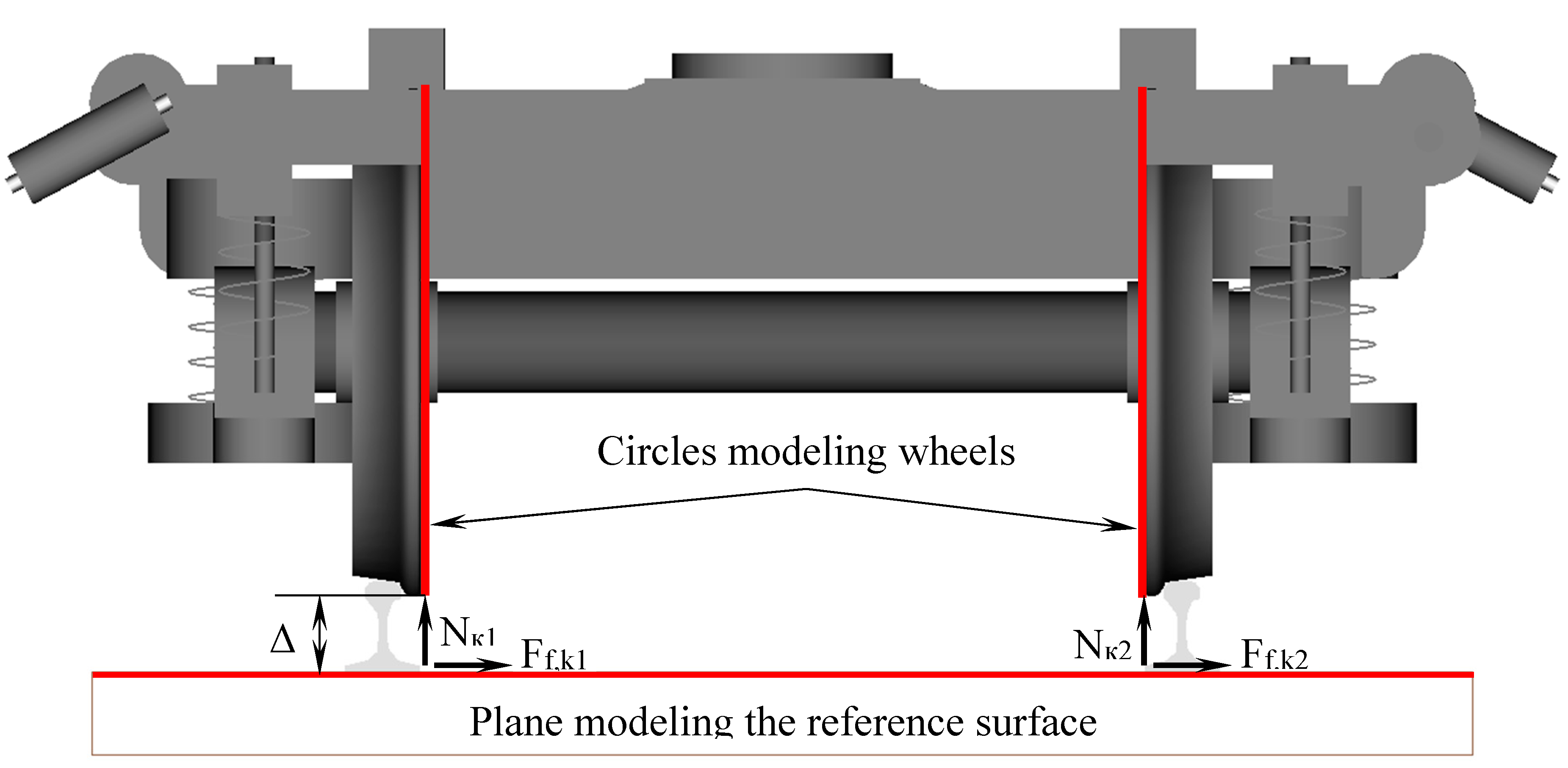
In other words, straight track widening is the transverse distance from the lowest point on the wheel's tread circle to the center point of the rail head in their ideal position [16]. Since when the bogies come off, all the wheels lose their contact with the rails, the model included elements that take into account the sliding (rolling) of the wheels on the supporting surface (see Figure 6).

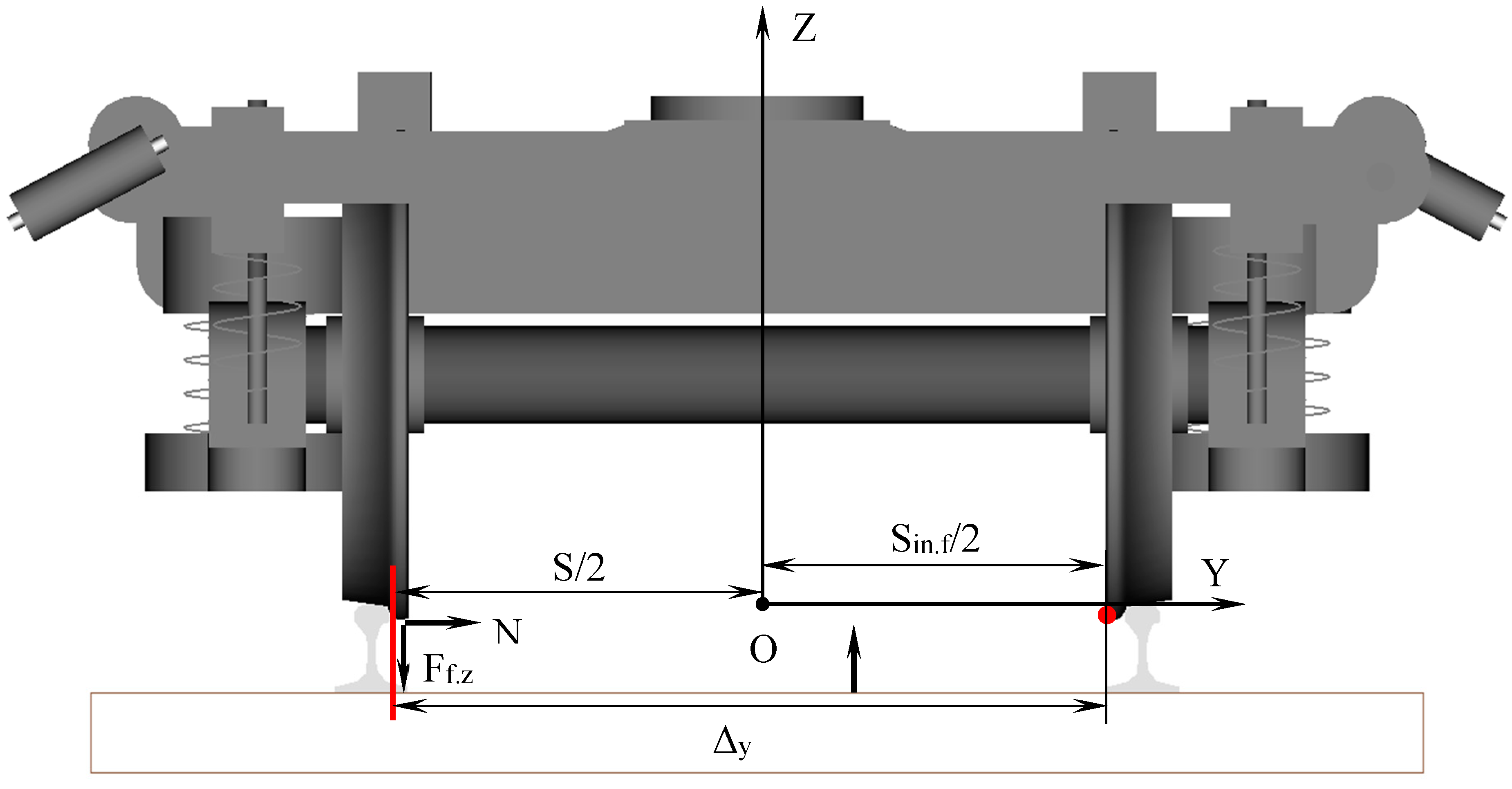
On Figure 7, for convenience of perception, only one interaction option is shown. In fact, the model also implements a symmetrical version of the interaction of the left wheel and the right rail, respectively [17].

Shown in Figure 6 and Figure 7, the schemes for the interaction of wheels with the ground surface and the side faces of the rails make it possible to limit the vertical and lateral movements of the wheels when they are completely derailed [18].

where N_ki – is the normal forces arising from contact with the supporting surface; ±F_f.ki– is the frictional forces that occur when contacting the ground; Δ – is the clearance between the bottom of the circle and the reference surface.

where N_рi, ±F_f.zi– is the normal forces and friction forces arising from the contact of the inner face of the right wheel with the inner face of the left rail; Δ_y – is the clearance between the inner edge of the wheel and the inner edge of the rail; S – is the track gauge; S_in.f– is the distance between the inner edges of the wheels

∆_{y} = \frac{S}{2} + \frac{S_{i n . f}}{2}

At the same time, it is assumed that the supporting surface is even, and the resistance to movement caused by the interaction of wheels with sleepers and crushed stone is set by additional forces applied to the wheelsets [19]. In order to take into account the longitudinal forces between the cars, automatic couplers and buffers were added to the model (see Figure 8 and Figure 9).

Figure 8. Coupler model diagram.

Figure 9. Scheme of the buffer device model.

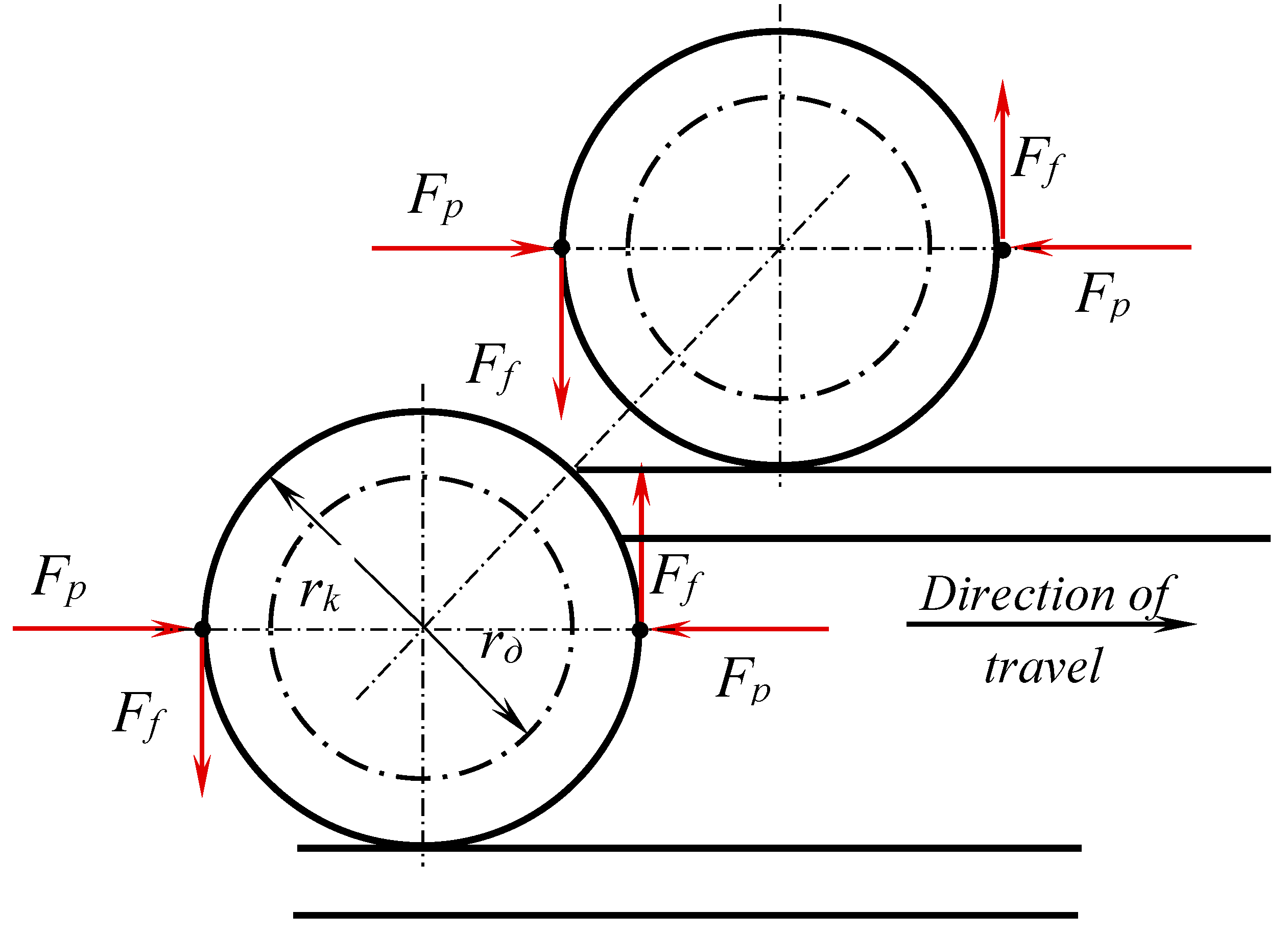
Figure 10. Scheme of forces on the wheelset, acting on double-sided pressing.

Braking forces were implemented using a moment tending to turn the wheel in the opposite direction (or stop the wheel) defined by the expression:

M_{b} = 4 F_{f} \cdot r_{k} = 4 F_{p} \cdot φ \cdot r_{k} (r_{\partial})

(12)

where F_f – is the frictional force between wheel and block, kN; F_p – is the pressing force per pad, kN; φ – is the coefficient of friction between wheel and rail; r_k – is the wheel radius, m.

In expression (12), the pressing force per one brake shoe can be determined from the expression:

F_{p} = i \cdot η (p_{c y} \cdot S \cdot η_{c y} - F_{s p}) / n_{k}

(13)

where i – is the gear ratio of the brake linkage is assumed to be 12 for passenger cars equipped with cast iron blocks [6]; η, η_cy – is the efficiency of the brake linkage and the brake cylinder is assumed to be 0.95 and 0.98, respectively; S – is the piston area of the passenger car brake cylinder is 0.0993 m²; F_sp– is the release spring force 2473 N; p_cy – is the pressure in the brake cylinder, Pa, is taken according to the braking indicator diagram, taking into account the features of filling the brake cylinder [20].

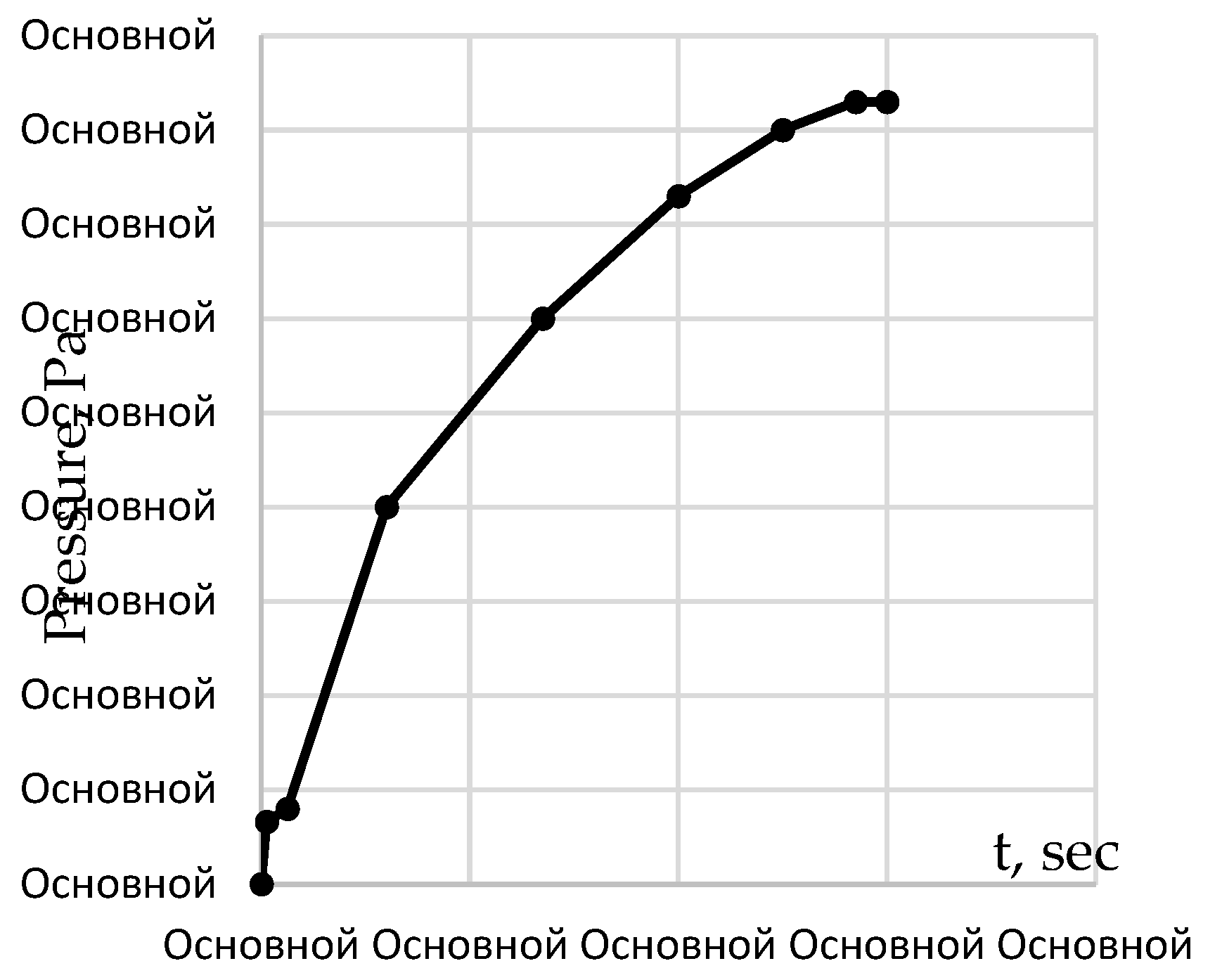
Based on the operational acts of measuring the filling time of the brake cylinders of passenger cars, the average filling time was taken to be 5.7 seconds. The brake cylinder filling indicator diagram is shown in Figure 11.

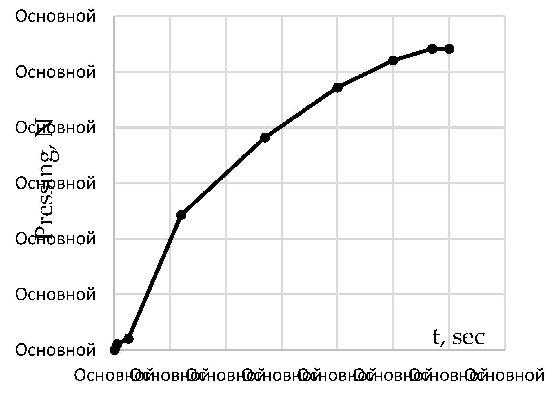
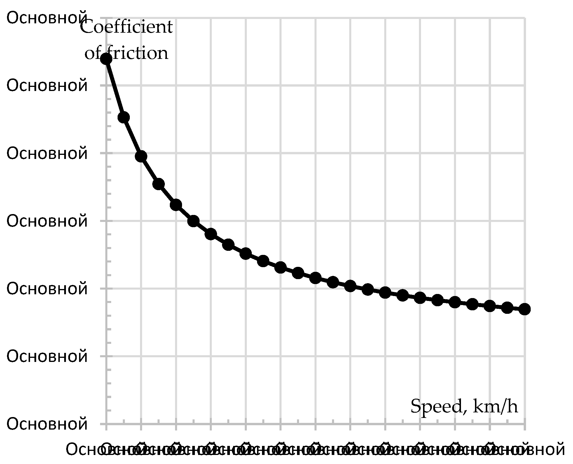
Using expression Eq. (13), we determine, in accordance with the filling diagram of the brake cylinder [21], the values of the pressing force on one brake shoe and build a brake pressure diagram (see Figure 12). The coefficient of friction between the cast-iron block and the wheel is determined by the expression for a constant value of the pressing force [7]:

ϕ = 0, 6 \frac{1, 6 F + 100}{8 F + 100} \cdot \frac{ν + 100}{5 ν + 100}

(14)

where F – is the pressing force, kN; ν – is the speed, km/h.

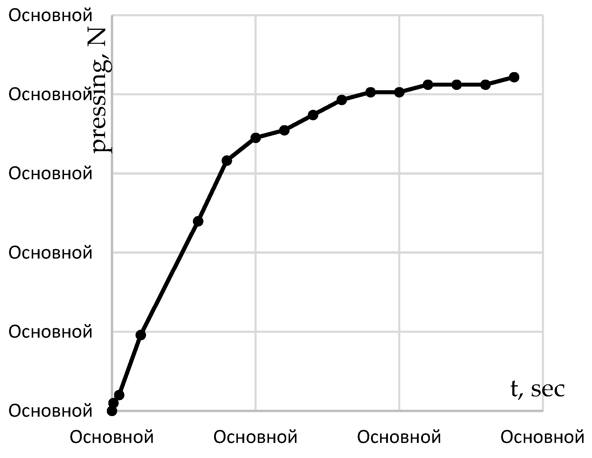
The total brake pressure on the axle of the locomotive wheelset was realized using the diagram shown in Figure 14, based on the data obtained when decoding the cassette of the KZ4AC electric locomotive in operation. Since a disc brake is used on electric locomotives of KZ4АC models [22], when calculating the moment of braking force 4F_p∙φ, applied to the axle of the wheel set of the locomotive and being its shoulder, in Eq. (12) instead of the radius of the wheel r_k, the radius of the middle axis of the brake disk r_д is taken [23].

Figure 13. The dependence of the coefficient of friction of a cast-iron brake pad on the speed of movement.

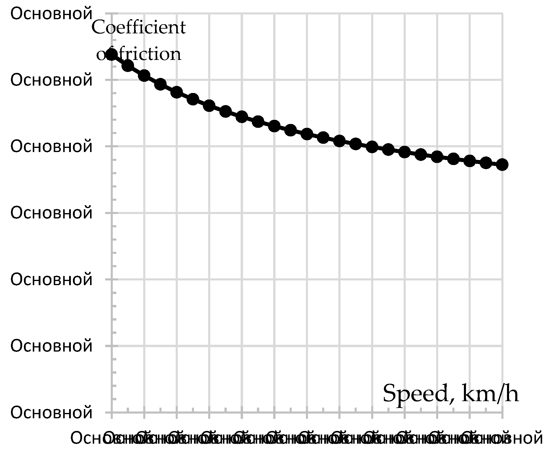
The coefficient of friction between the composite block and the wheel is determined by the expression for a constant value of the pressing force [7]:

ϕ = 0, 44 \frac{F + 20}{4 F + 20} \cdot \frac{ν + 150}{2 ν + 150}

(15)

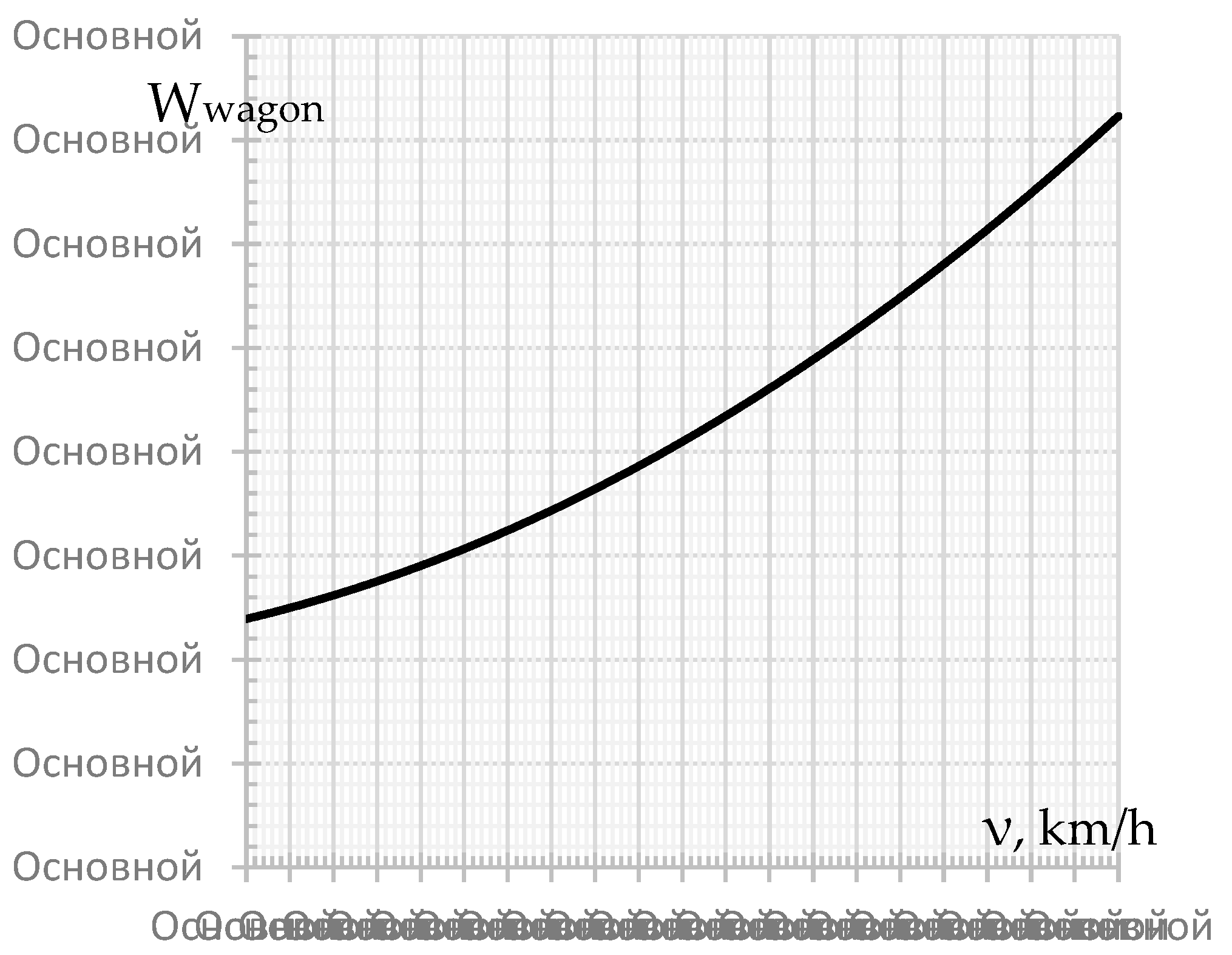
As is known from the rules for traction calculations [6], the main specific resistance to the movement of a passenger car on a seamless track is determined from the expression:

W_{w a g o n} = 0, 7 + \frac{8 + 0.16 ν + 0, 0023 ν^{2}}{q_{0}}

(16)

where

q_{0} = \frac{m_{w a g o n}}{4}

– is the axle load in tons. m_wagon – is the average weight of a fully equipped wagon is assumed to be 64.475 tons [24].

The main specific resistance to the movement of the locomotive in the coast down mode on a seamless track is determined from the expression:

W_{l o c o m o t i v e} = 2, 4 + 0, 009 ν + 0, 00035 ν^{2}

(17)

Figure 15. The dependence of the coefficient of friction of the composite brake pad on the speed of movement.

Figure 16. The main specific resistance to the movement of the car.

Having done elementary transformations of expressions Eq. (16) and Eq. (17), we pass from a dimensionless quantity to a force quantity in Newton’s:

W_{w a g o n} = g \cdot (0, 7 + \frac{8 + 0, 16 ν \cdot 3, 6 + 0, 0023 {(ν \cdot 3, 6)}^{2}}{q_{0}}) \frac{m_{w a g o n}}{1000}

(18)

W_{l o c o m o t i v e} = g \cdot (2, 4 + 0, 009 ν \cdot 3, 6 + 0, 00035 {(ν \cdot 3, 6)}^{2}) \frac{m_{l o c o m o t i v e}}{1000}

(19)

where g – is the gravitational acceleration, m/s².

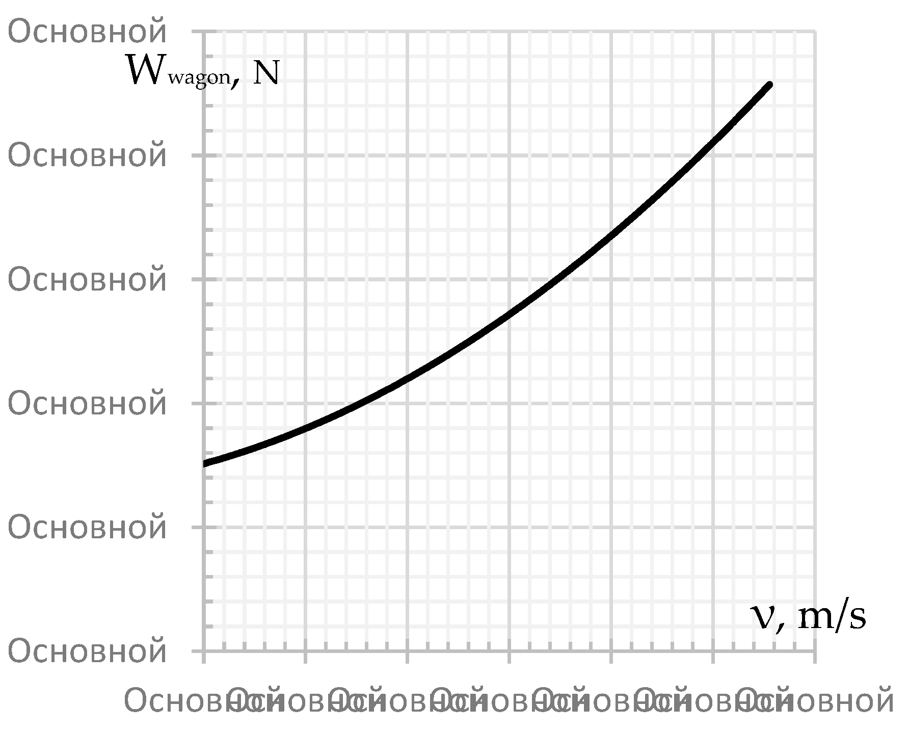
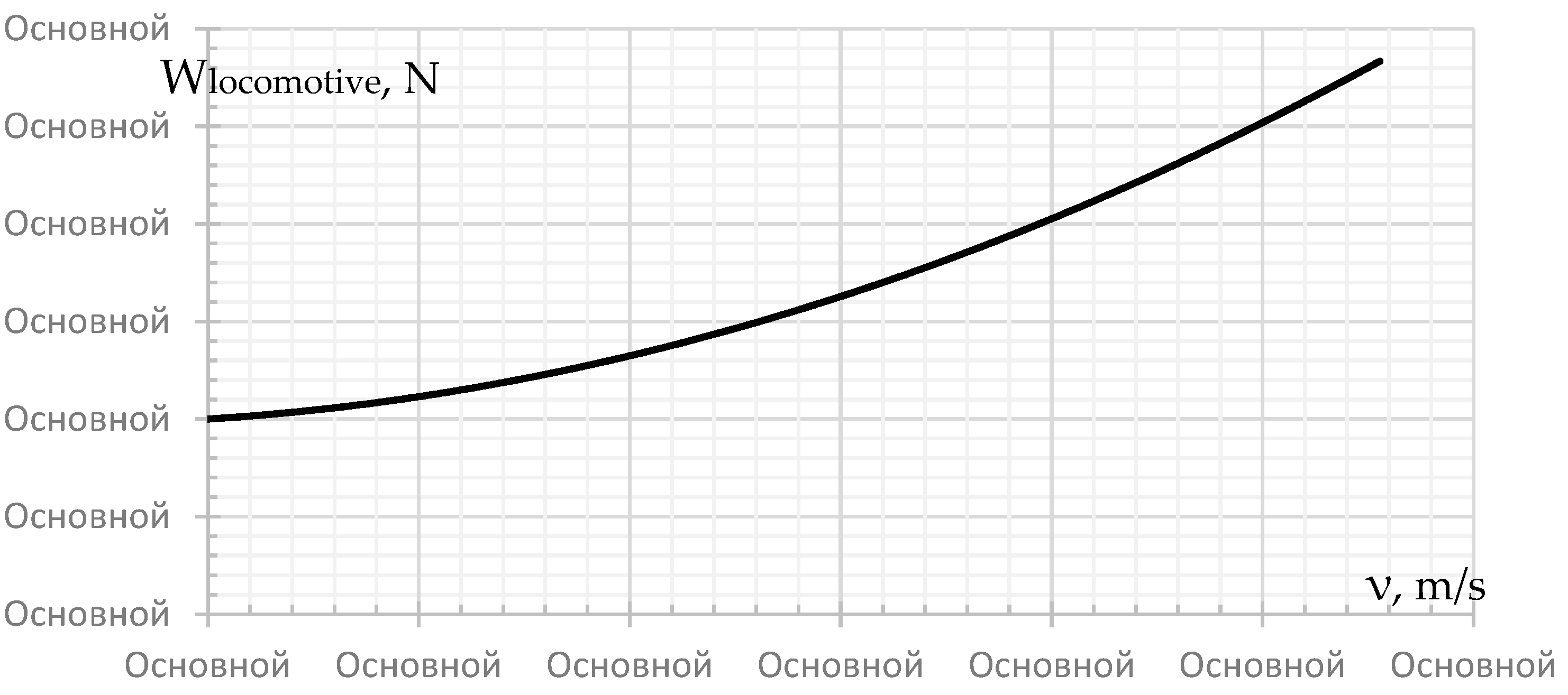
Dependences of the dimensionless and recalculated in Newton’s of the main specific resistance of movement on speed are shown in Figure 17, Figure 18 and Figure 19. Forces that simulate resistance to movement are applied to the centers of gravity of each unit of rolling stock and are directed against the direction of movement [25].

3. Results (Motion Simulation)

Experimental studies and modeling of the behavior of railway vehicles in the braking mode have been given attention by various authors [9]. Before modeling the movement of the entire train, which takes significant computing resources, a series of calculations was carried out using single models [26]. At the same time, longitudinal and braking forces were not taken into account at this stage, since their influence on an individual crew is very small. When determining the causes of rolling stock derailment, as a rule, the main criterion to be assessed is the wheel derailment stability factor (the tendency of the wheel to “crawl” with the flange onto the rail head), which is based on the consideration of the wheel balance equations under conditions of contact with the flange:

λ = \frac{t g β - μ}{μ \cdot t g β + 1} \cdot \frac{P_{v e r 1}}{P_{h o r}} \geq [λ_{n o r m a l}]

(20)

where β – is the angle of inclination of the ridge generatrix of the cone-shaped surface of the wheel with the horizon, rad.; μ – is the coefficient of friction of interacting surfaces of wheels and rails; P_ver1 – is the coefficient of friction of interacting surfaces of wheels and rails, N; P_hor – is the horizontal component of reaction forces of the running wheel on the rails, N; [λ_normal] – is the admissible value of the safety factor of the wheelset stability against derailment.

Lateral and frame forces are also important indicators that evaluate the force effect of the crew on the track. Exceeding the normative values of these forces can cause the destruction of the track and the derailment of the crew [27]. The maximum allowable values of frame forces are calculated from the condition of stability of the rail-sleeper grid of the track from transverse shear along the ballast under the influence of the frame force as the ratio of the frame force Н_рk to the axial load Р₀ (Н_р/Р₀). Normalized values of the mentioned indicators are given in Table 1.

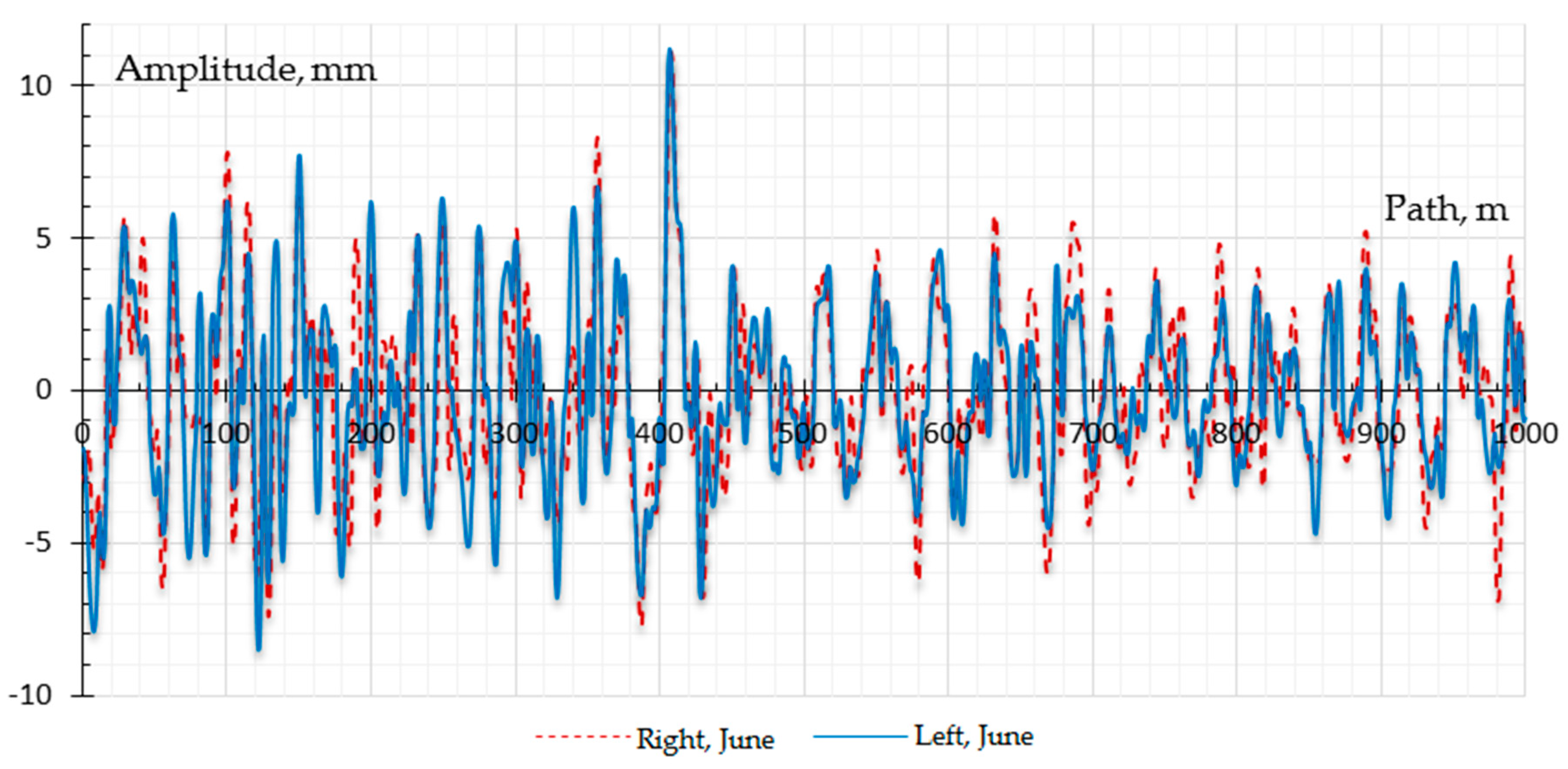
To calculate the lateral forces, the totality of all forces acting on the wheel during contact interaction with the rail at all points of contact is used. In addition, when analyzing wheel derailment, the transverse displacements of wheel sets relative to the track axis are additionally evaluated [28]. It is obvious that, due to the increased inertial parameters, the locomotive will definitely pass, without rolling the wheels onto the rail head, the irregularities, during the passage of which the passenger car will derail. In this regard, the simulation of the situation of the derailment of the locomotive was not carried out. At the same time, assuming that the effect of vertical irregularities on horizontal oscillations is insignificant, vertical irregularities with an “excellent” rating were used in the calculations. The numerical values of the irregularities taken by the track measuring car for 1500 km of the considered section of the track are shown in Figure 20.

Figure 20. Horizontal irregularities of rail threads 1500 km.

Figure 21. Horizontal irregularities of rail threads 1-2 wheel pair (WP) 1500 km.

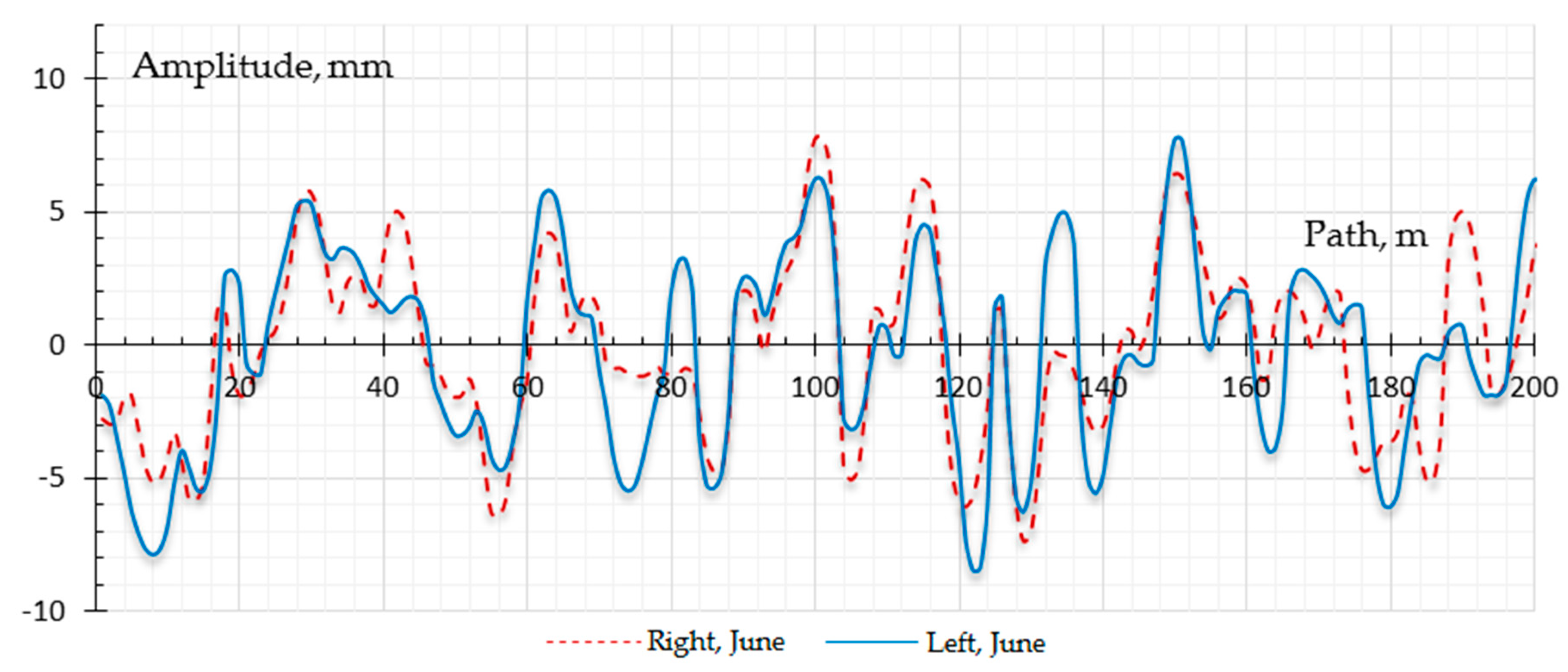
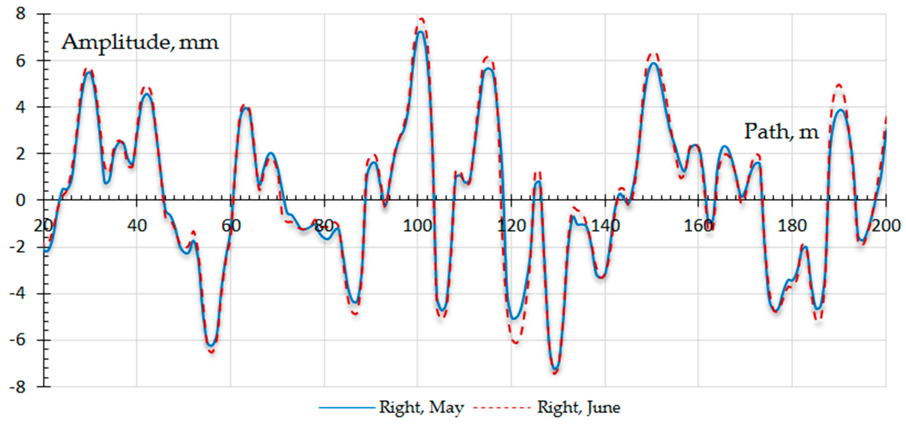
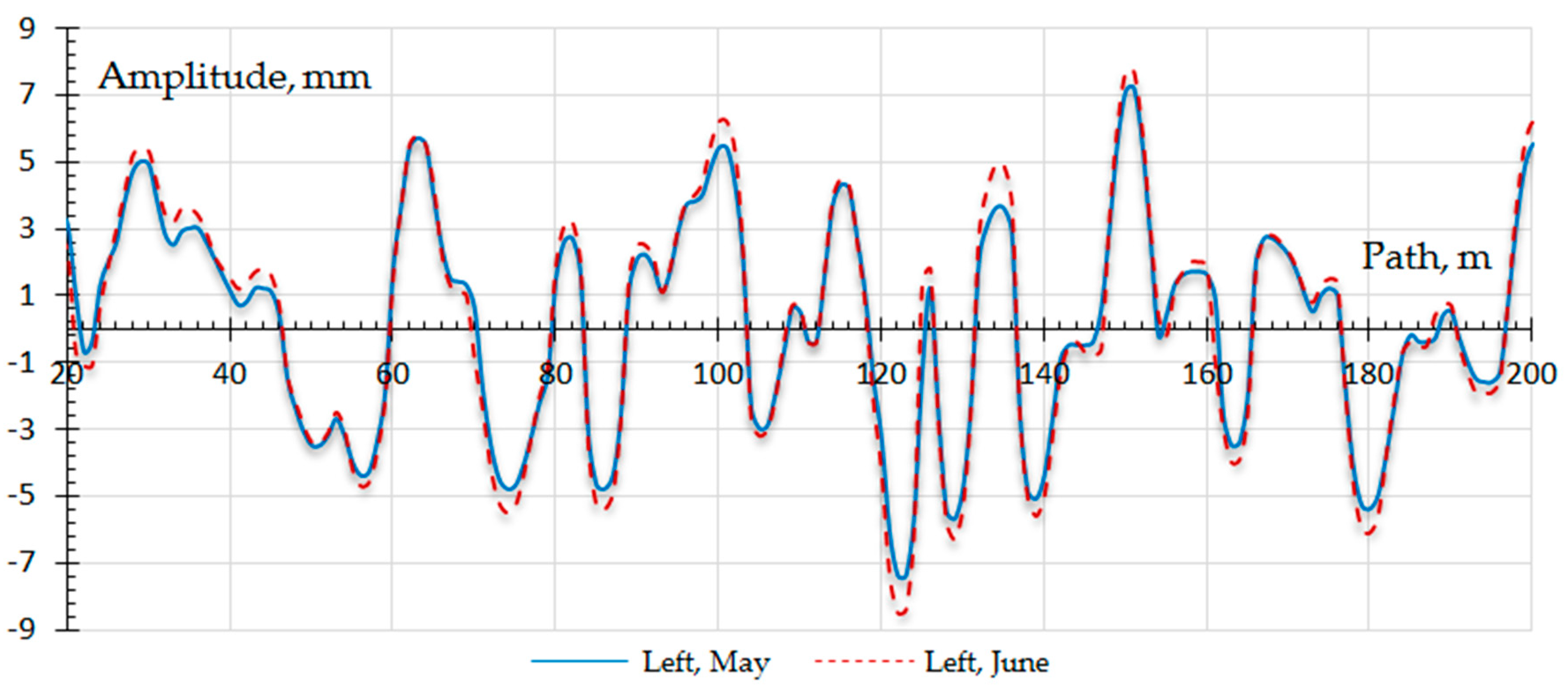
Figure 22 and Figure 23 show the roughness of the right and left rail threads for May and June, respectively, since, in order to simplify, we perform the simulation for these months. Simulations during the fall and winter months should take into account the effects of climate and weather factors, such as snow or rainfall, in order to obtain more accurate data [29].

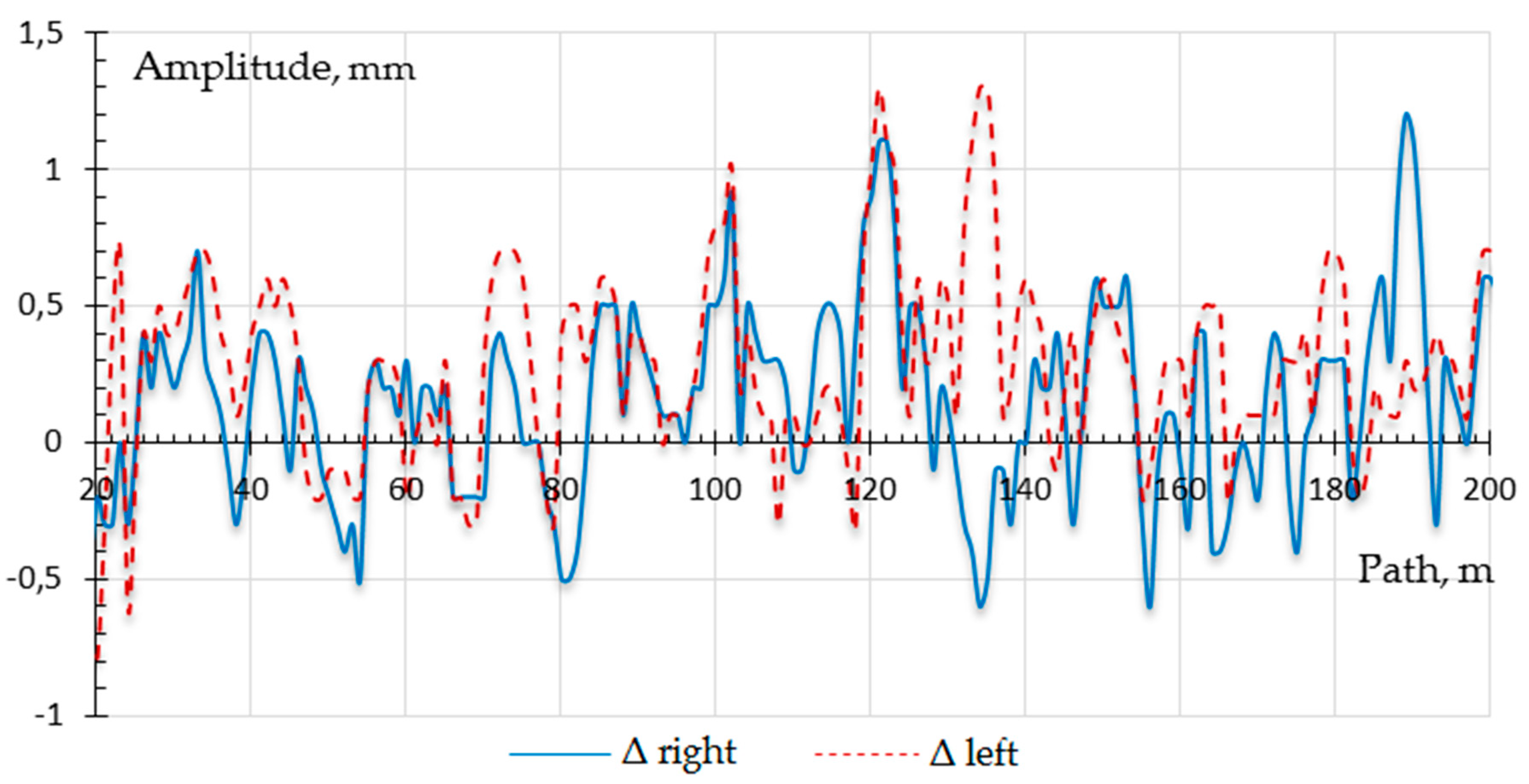
In addition, Figure 25 shows the change in the amplitudes of the irregularities of the rail threads for a month. In this case, negative values correspond to a decrease in the roughness amplitude.

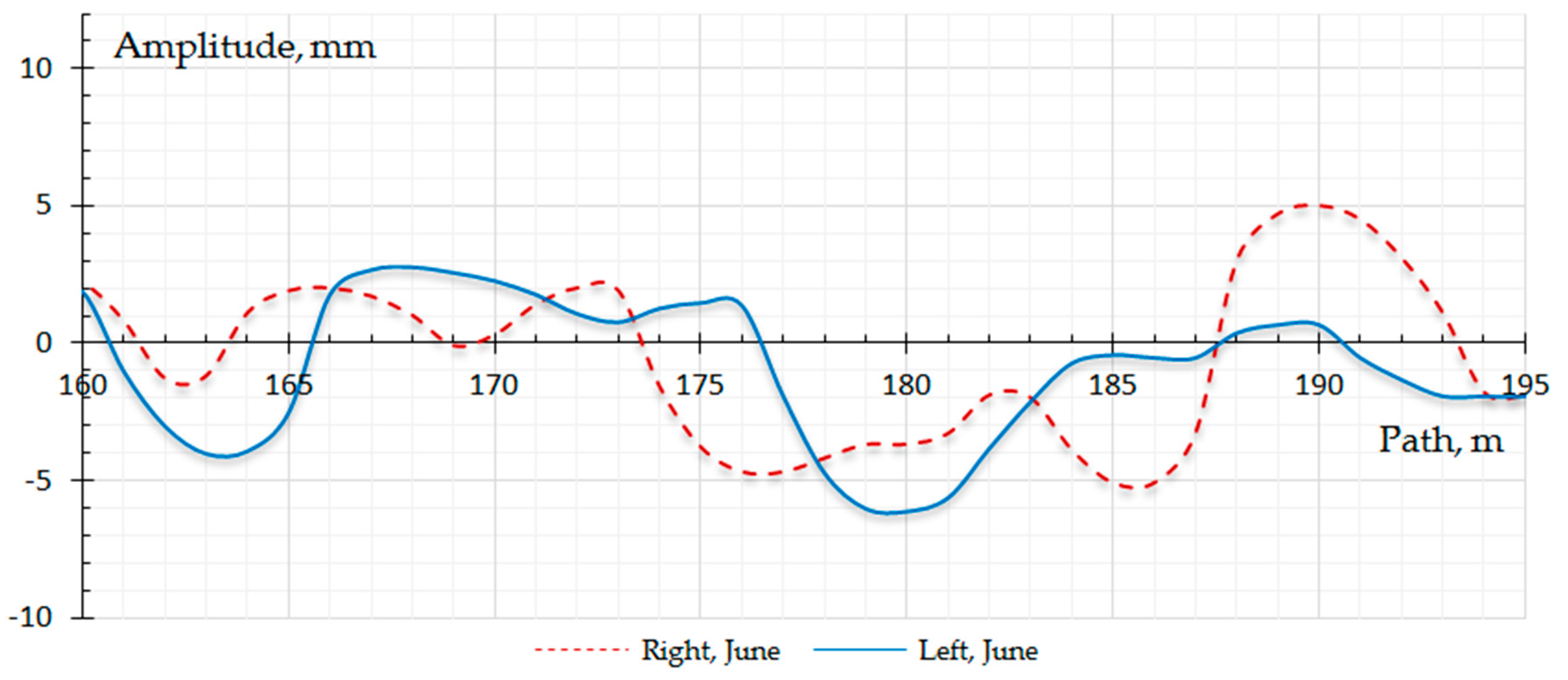
From Figure 22, Figure 23, Figure 24 and Figure 25 it can be seen that the periods of irregularities for 1-2 wheel pair (WP) are in the range from 5 to 14 m. In addition, on a segment of 160-190 km, a mismatch between the periods along the right and left rail threads is noticeable (see Figure 25).

Figure 24. Change in the amplitudes of the irregularities of the rail threads for one month.

Figure 25. Irregularities of rail threads at 160-195 m 2 wheel pair (WP).

Taking into account the analysis of the stability of the track based on the results of the passages of the track measuring car and in the Comprehensive pre-failure analysis (CPFA) seamless path (SP) resource management, risk management and reliability analysis (RMMRA) software package, it was assumed that at 2-3 wheel pair (WP), due to temperature forces, an uneven track occurred, which, according to [6,7,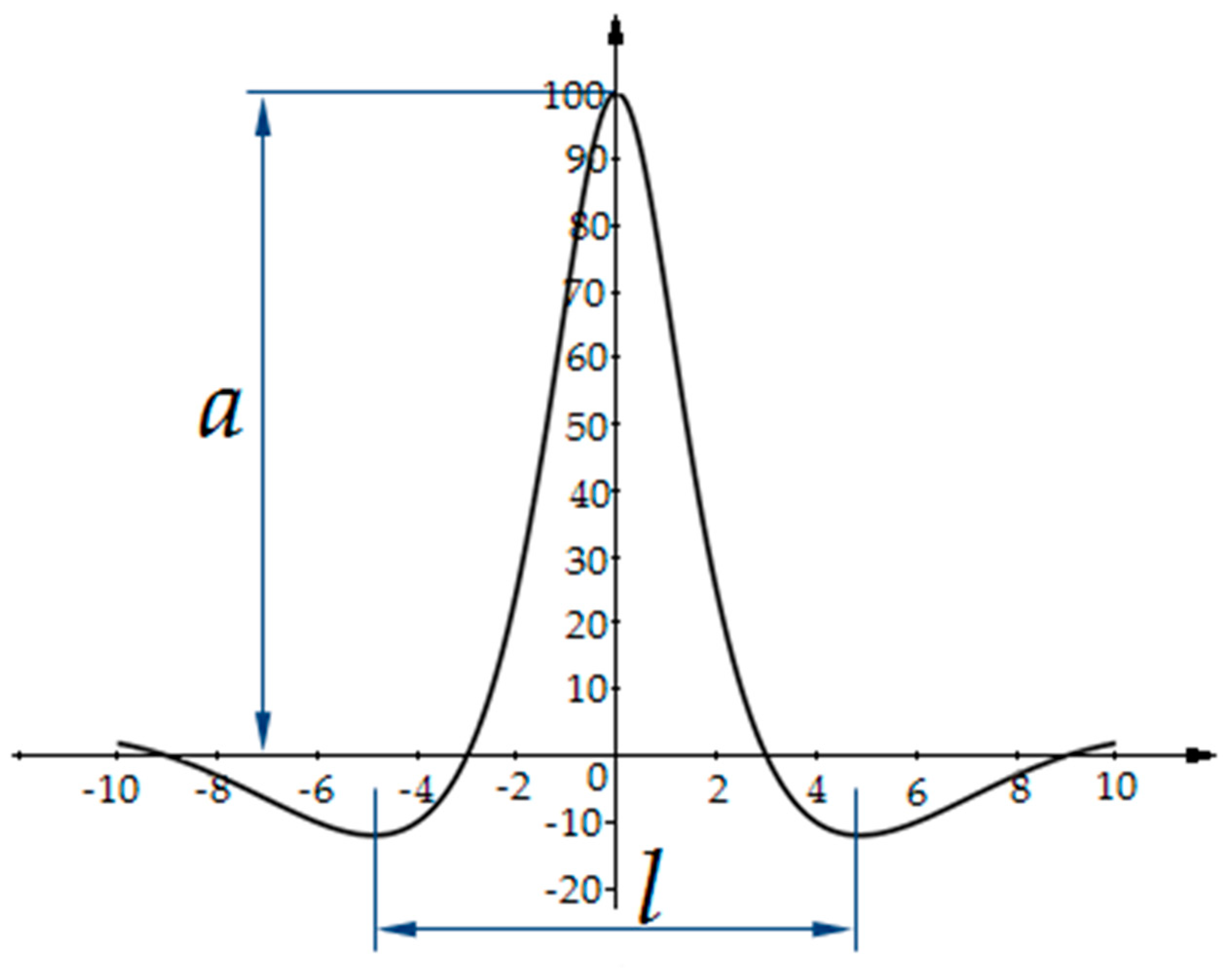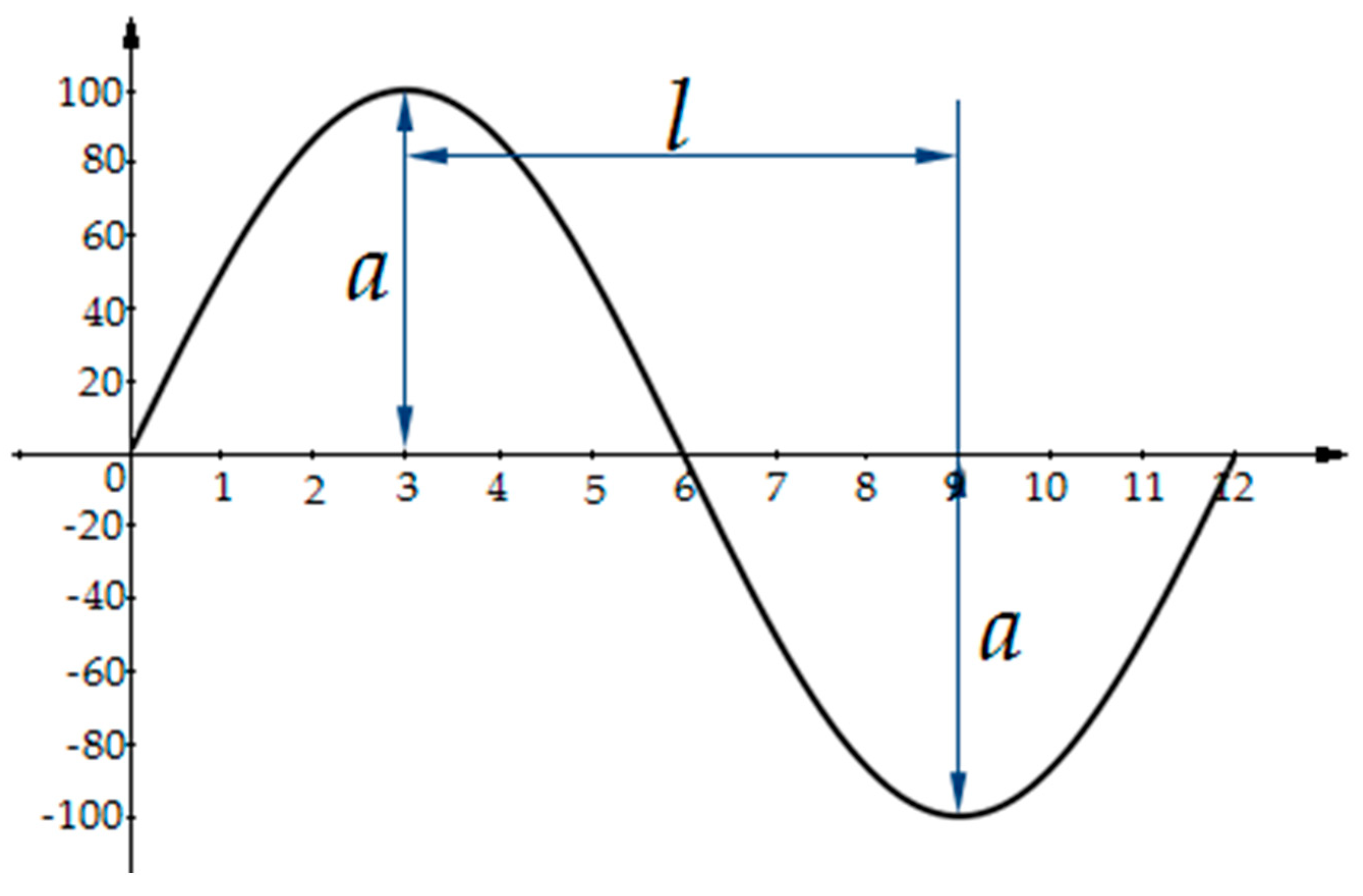8] on a straight section of the track could have the forms shown in Figure 26 and Figure 27.

In Figure 26 and Figure 27, а – is the coefficient taking into account the amplitude; L – is the coefficient taking into account the length; b – is the coefficient taking into account damping.

It is obvious that it is not possible to fully simulate (repeat) the process of emergency braking or derailment of a train using simulation methods, since the derailment of the rolling stock is affected by many factors that, alas, cannot always be taken into account by mathematical methods (for example, a change in the shape of an unevenness due to temperature in time, with simultaneous movement of the railway vehicle along the given irregularity). In this regard, in order to accurately describe the derailment process, for example, after emergency braking, it is necessary to resort to a deductive and inductive analysis of the results of modeling local models of rolling stock and trains, which make it possible to identify the influence of one or another factor on traffic safety [29].

So, using the data given in Table 2, a train model was formed, consisting of a locomotive and 20 wagons (see Figure 28).

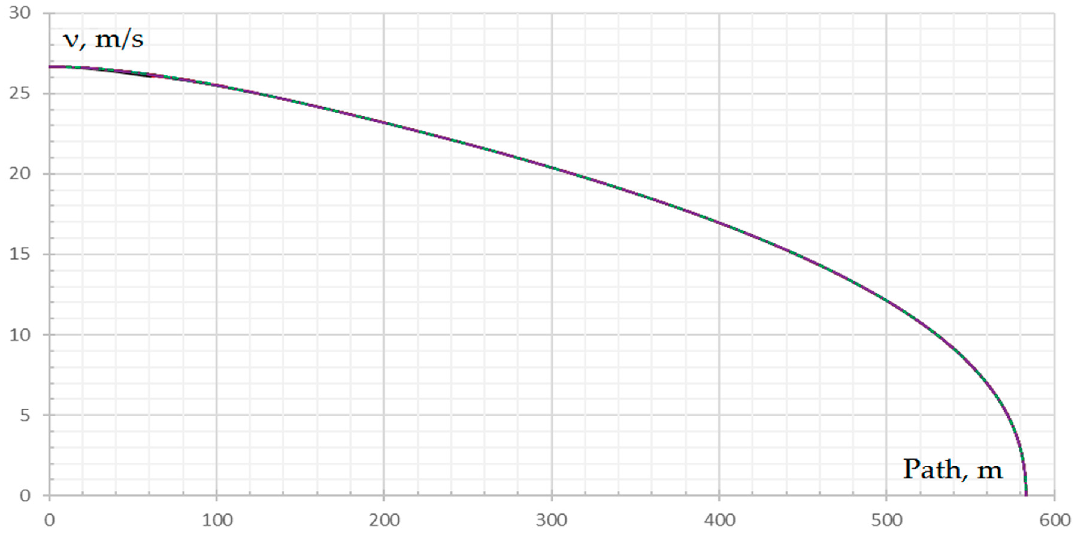
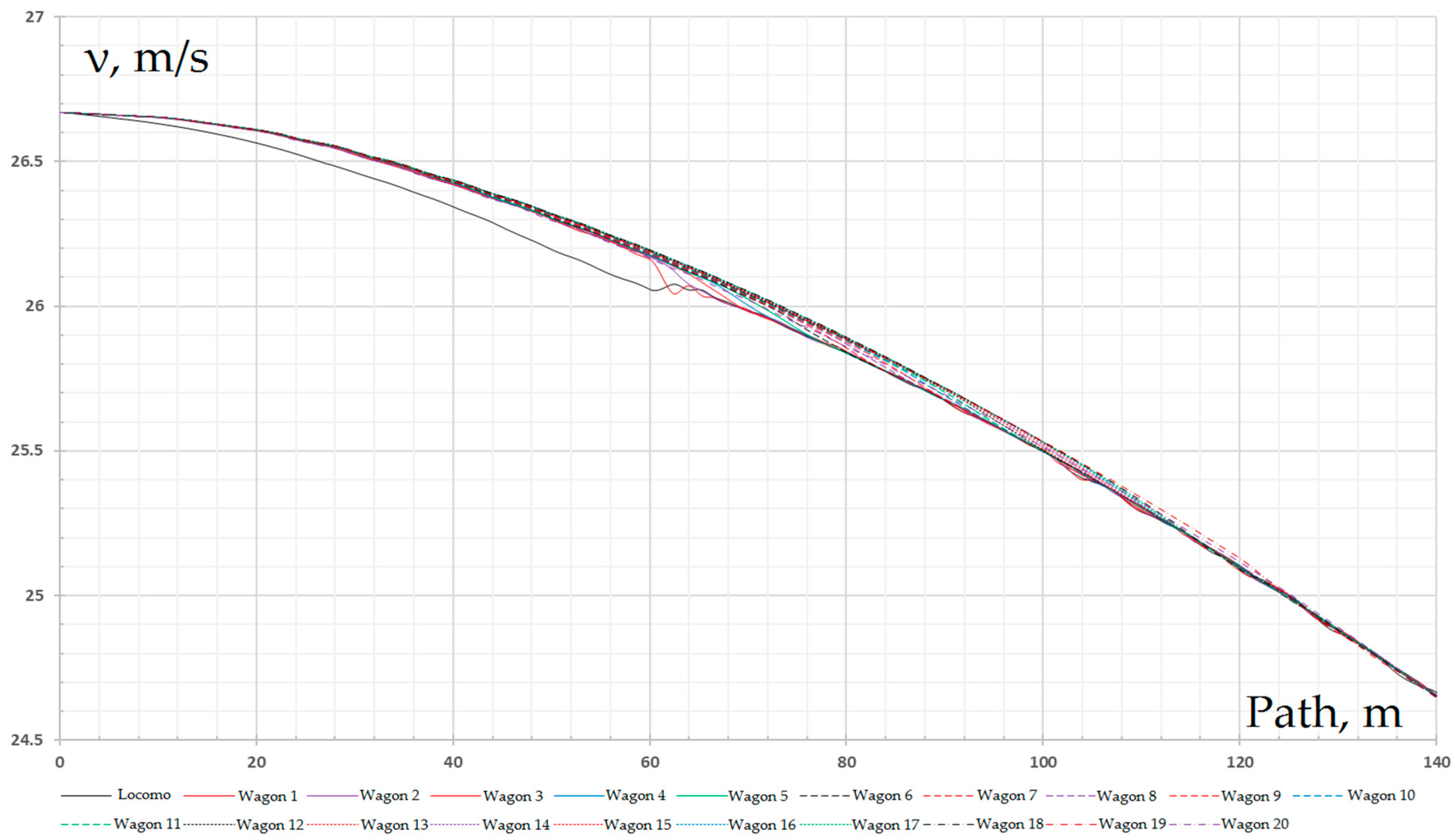
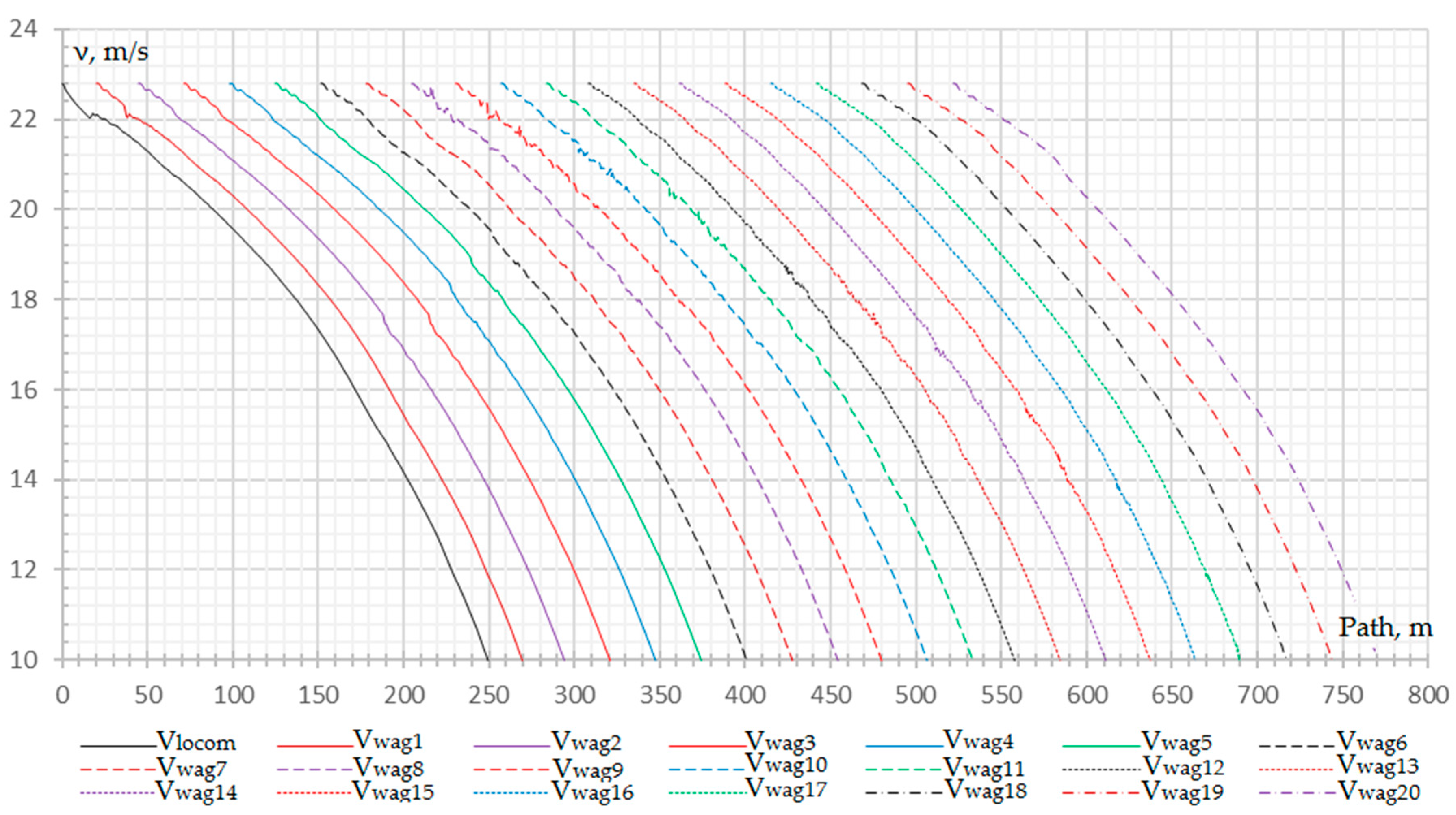
With the help of the generated model, the calculated braking distance of the train was determined and the longitudinal forces between the automatic couplers of adjacent cars were analyzed, in the state of the track with irregularities shown in Figure 20, Figure 21, Figure 22, Figure 23, Figure 24 and Figure 25. Figure 29 shows the decrease in the speed of rolling stock units depending on the distance traveled during braking. The braking distance was 583 m from the moment the emergency braking was applied. This value is within the normal range according to melt flow index (MFI) [6]. Figure 30 shows the section of the speed reduction graph where the transient occurs.

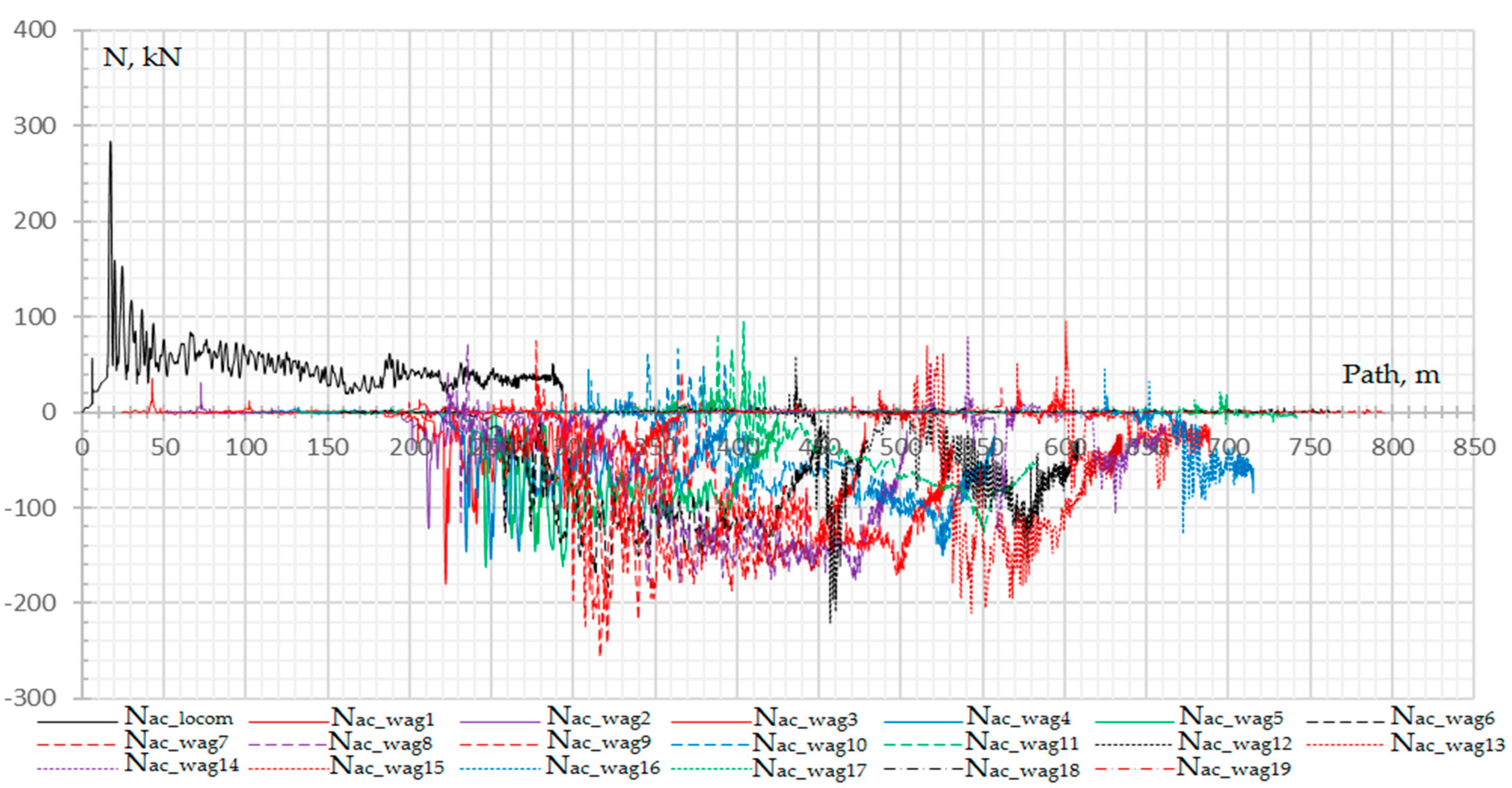
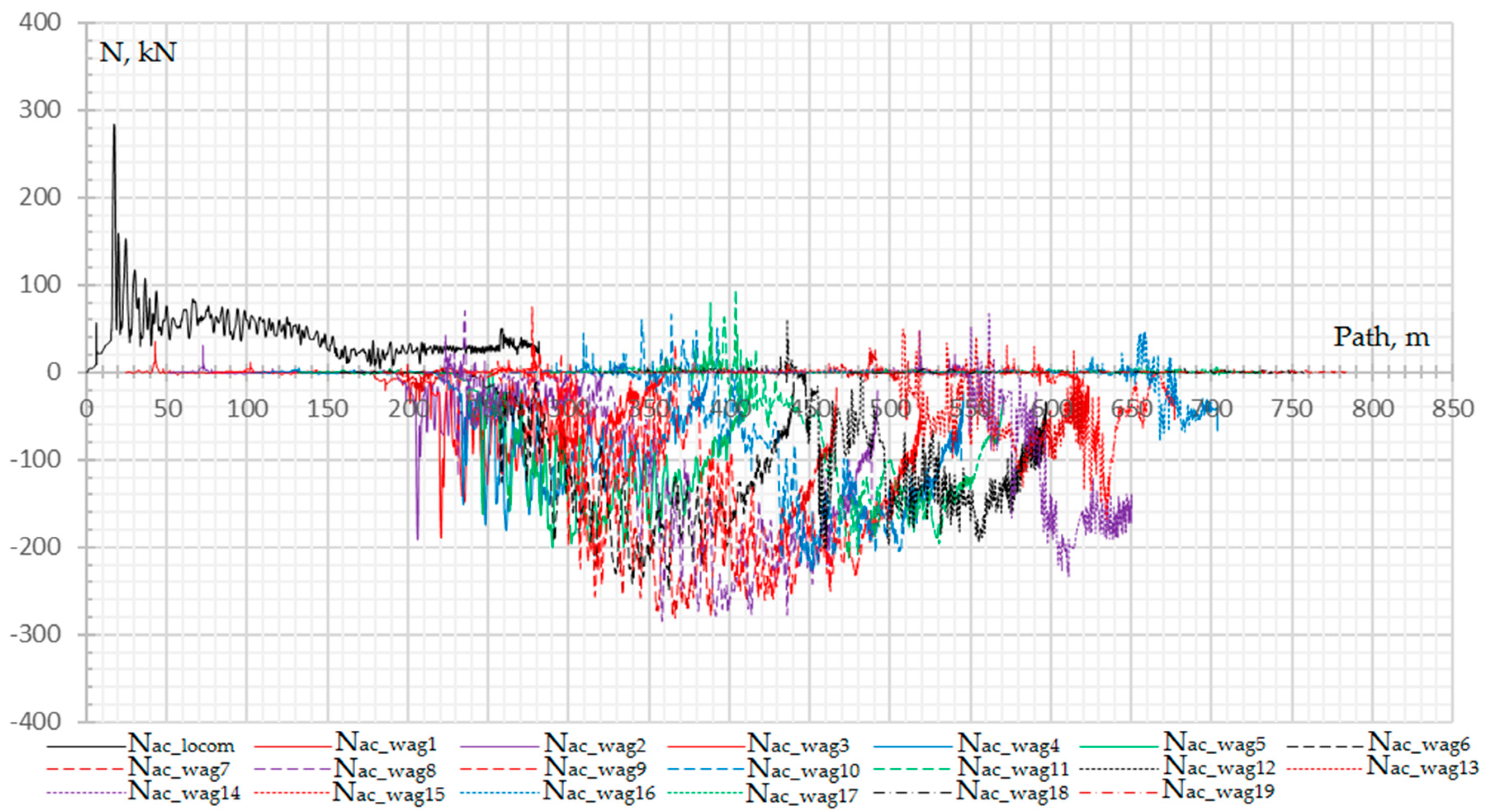
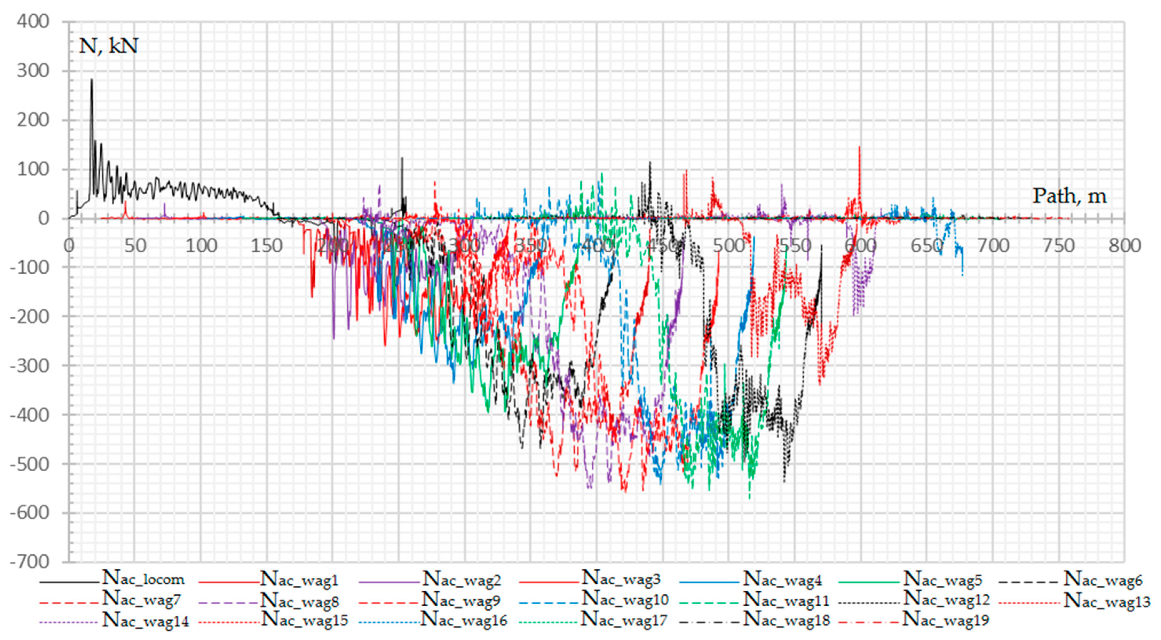
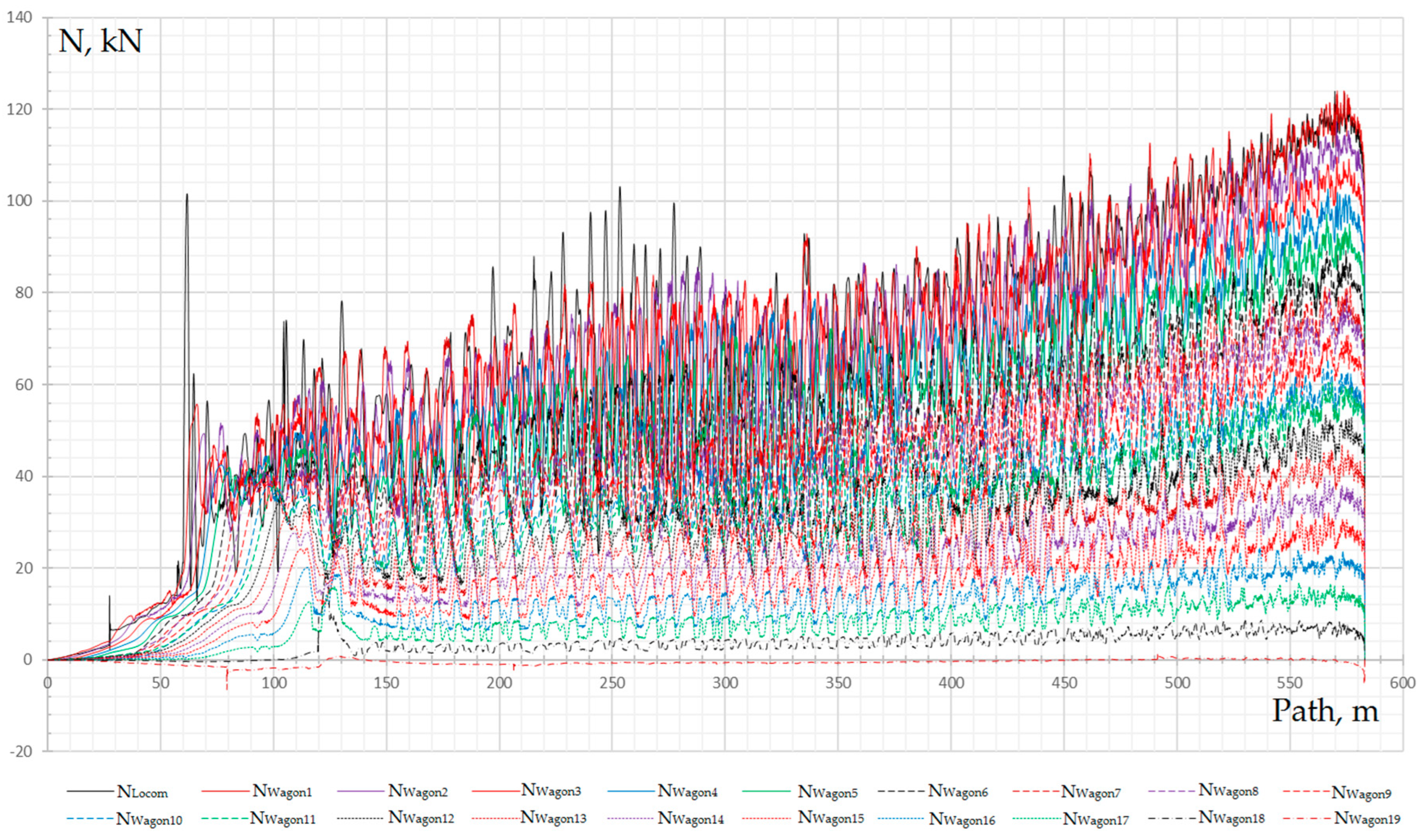
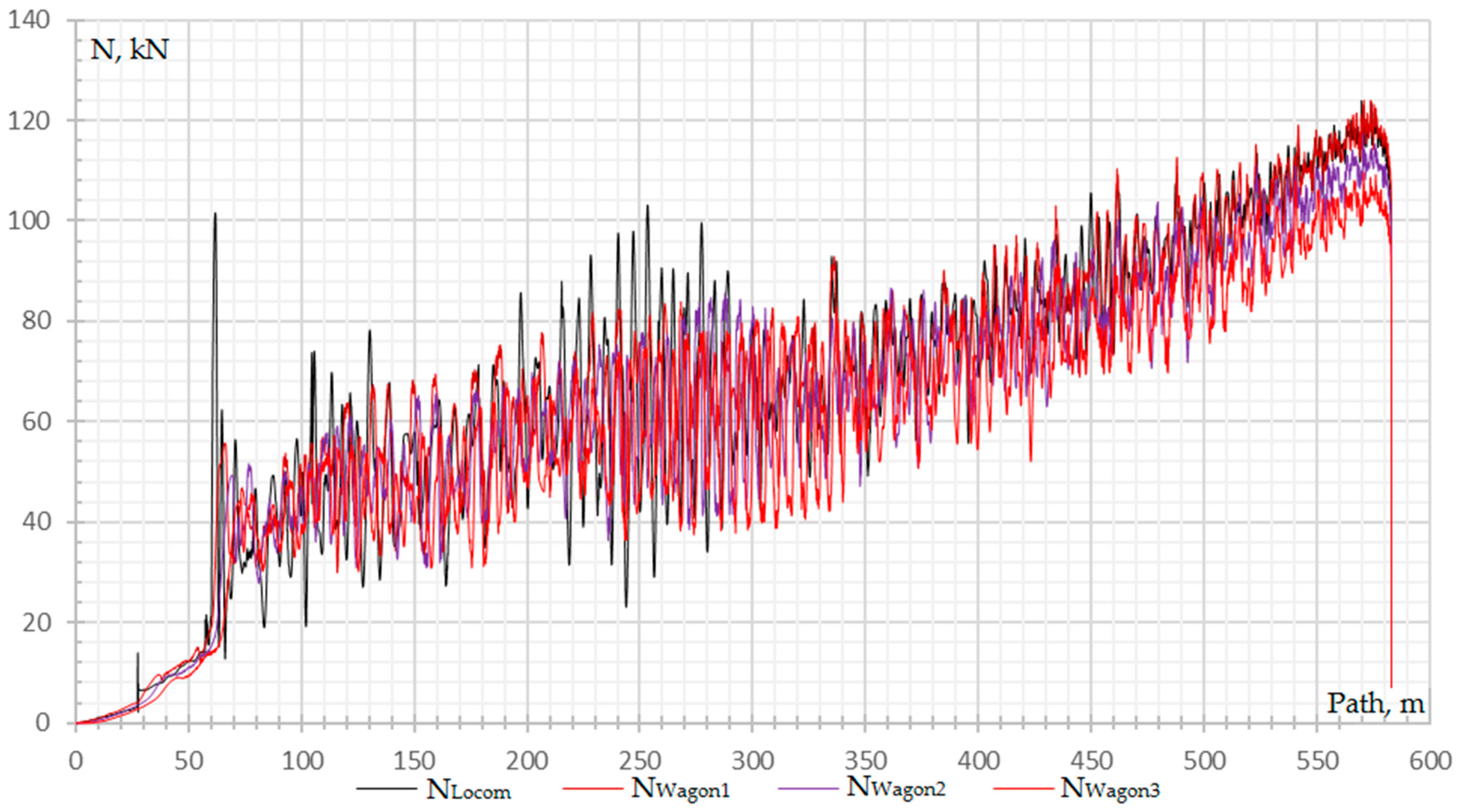
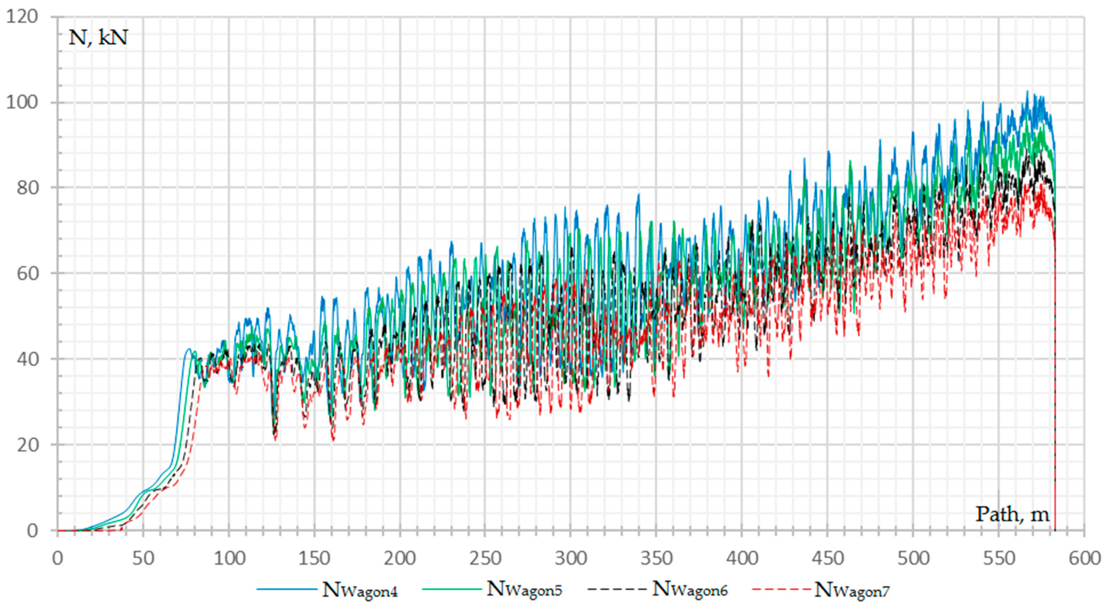
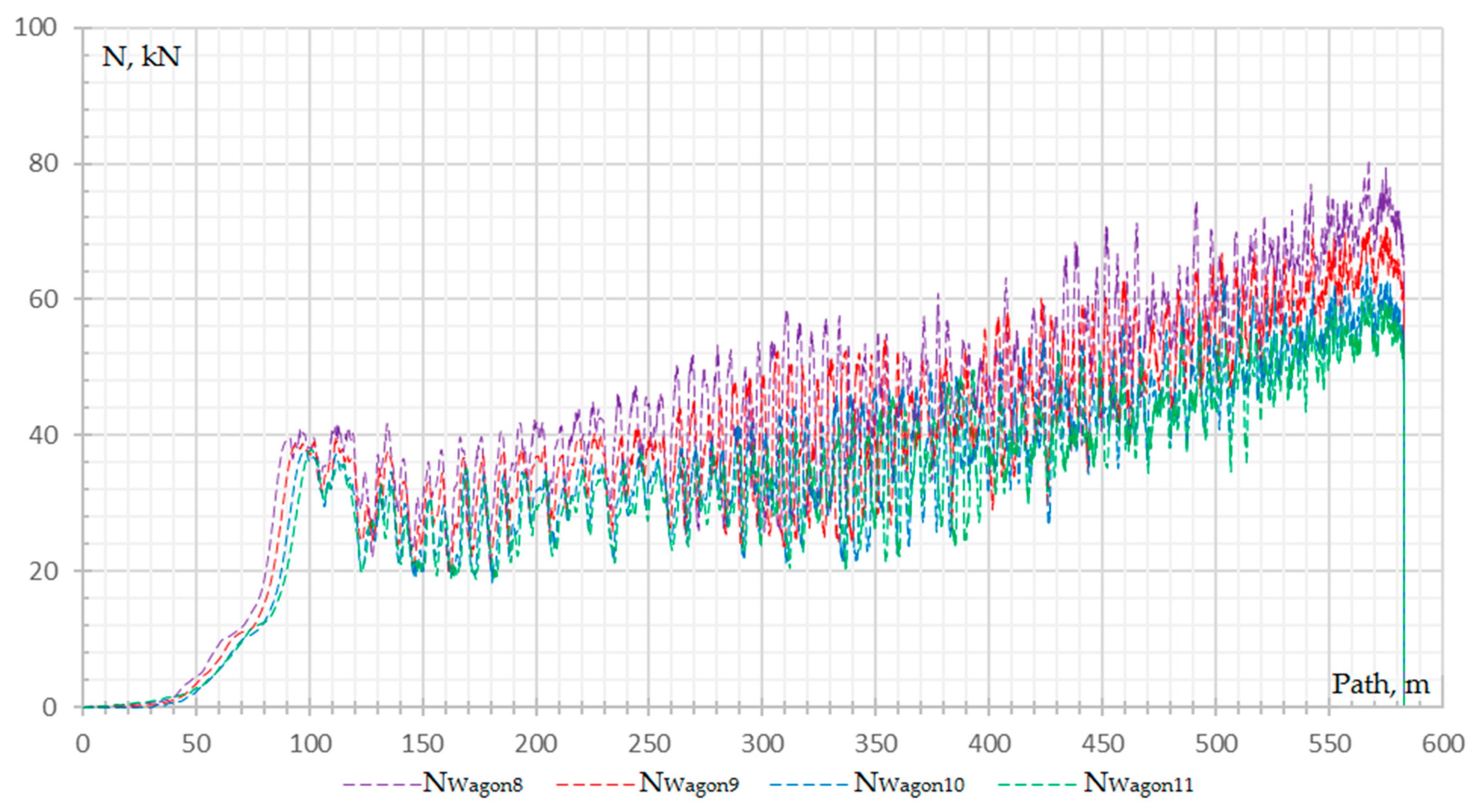
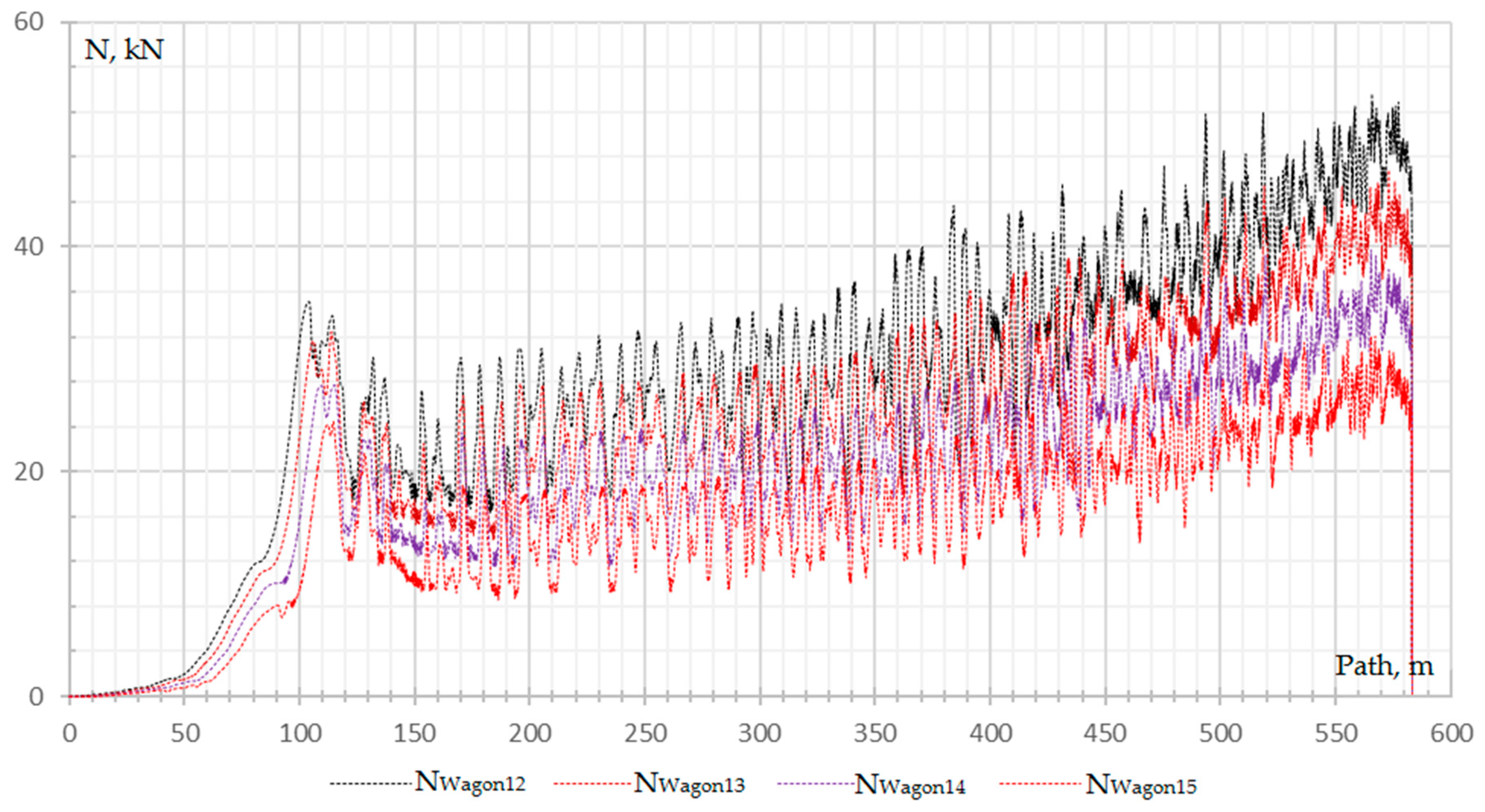
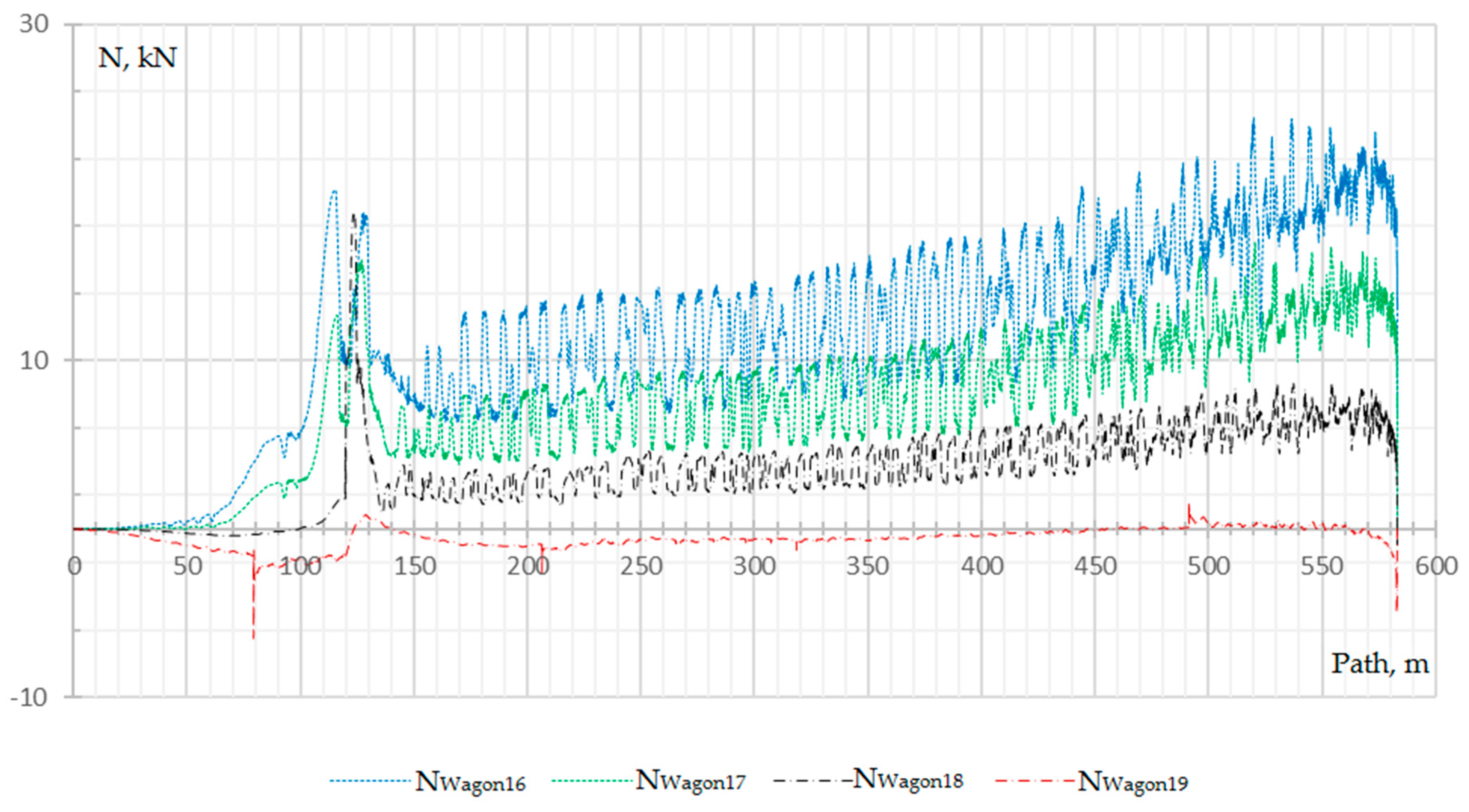
Figure 31, Figure 32, Figure 33, Figure 34 and Figure 35 show oscillograms of the total longitudinal forces between adjacent rolling stock units depending on the distance traveled. Due to the presence of buffer devices, braking is shockless, except for the connection between the locomotive and the first car.

The total longitudinal force between rolling stock units is determined by the formula:

N_{s u m i} = N_{A C i} + \sum N_{b i}

(21)

where N_АС_i – is the longitudinal force in the tail coupler of the i-th rolling stock unit; ∑N_bi – is the sum of the longitudinal forces in the tail buffer devices of the cars.

An analysis of the oscillograms showed that the transient compression process occurs up to 150 m, and then the process proceeds in a steady state. At the same time, Figure 36 shows that, due to the reduced mass, the last car lags behind the other cars in speed, as evidenced by the tensile forces between the last and penultimate cars.

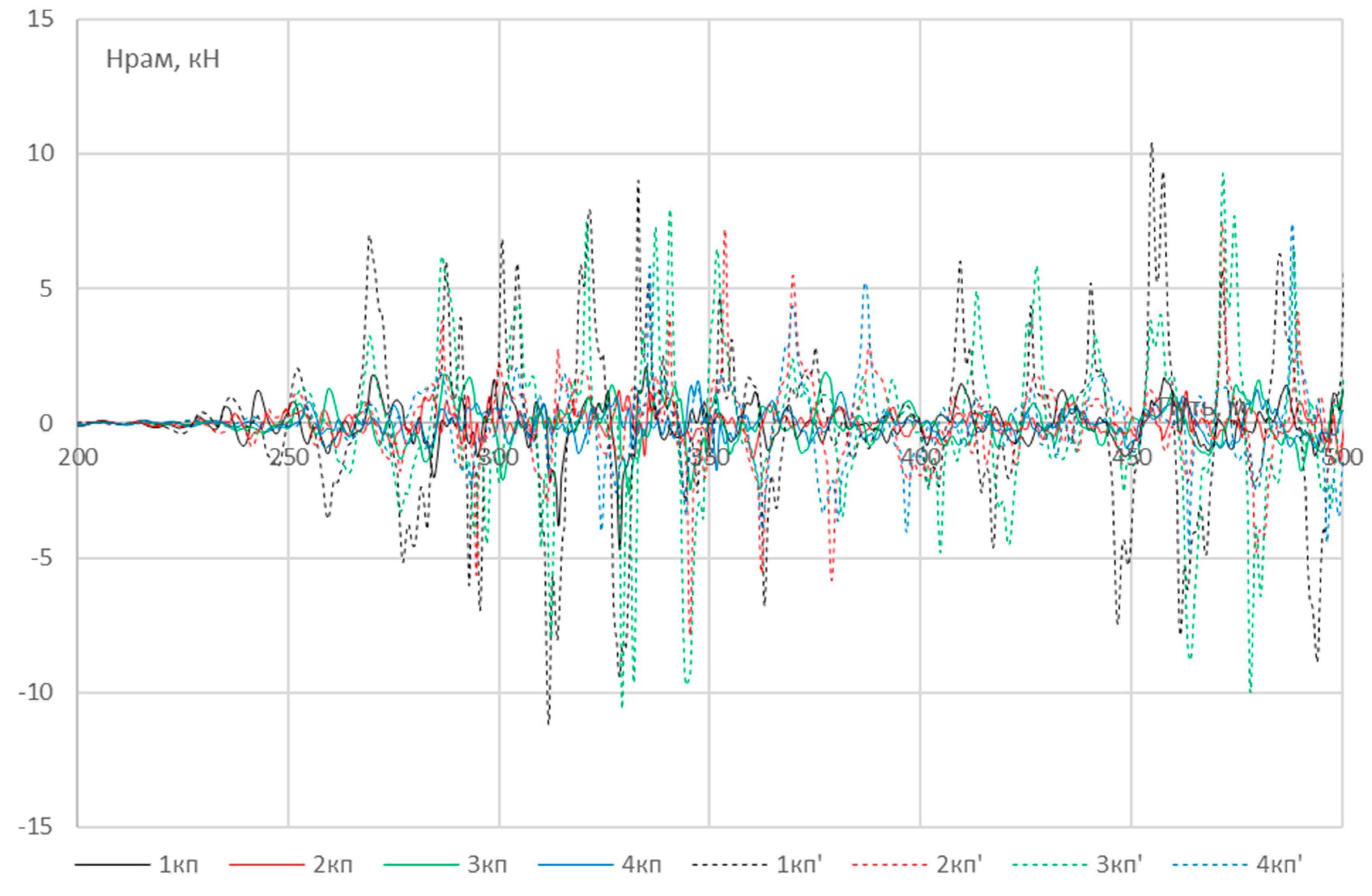
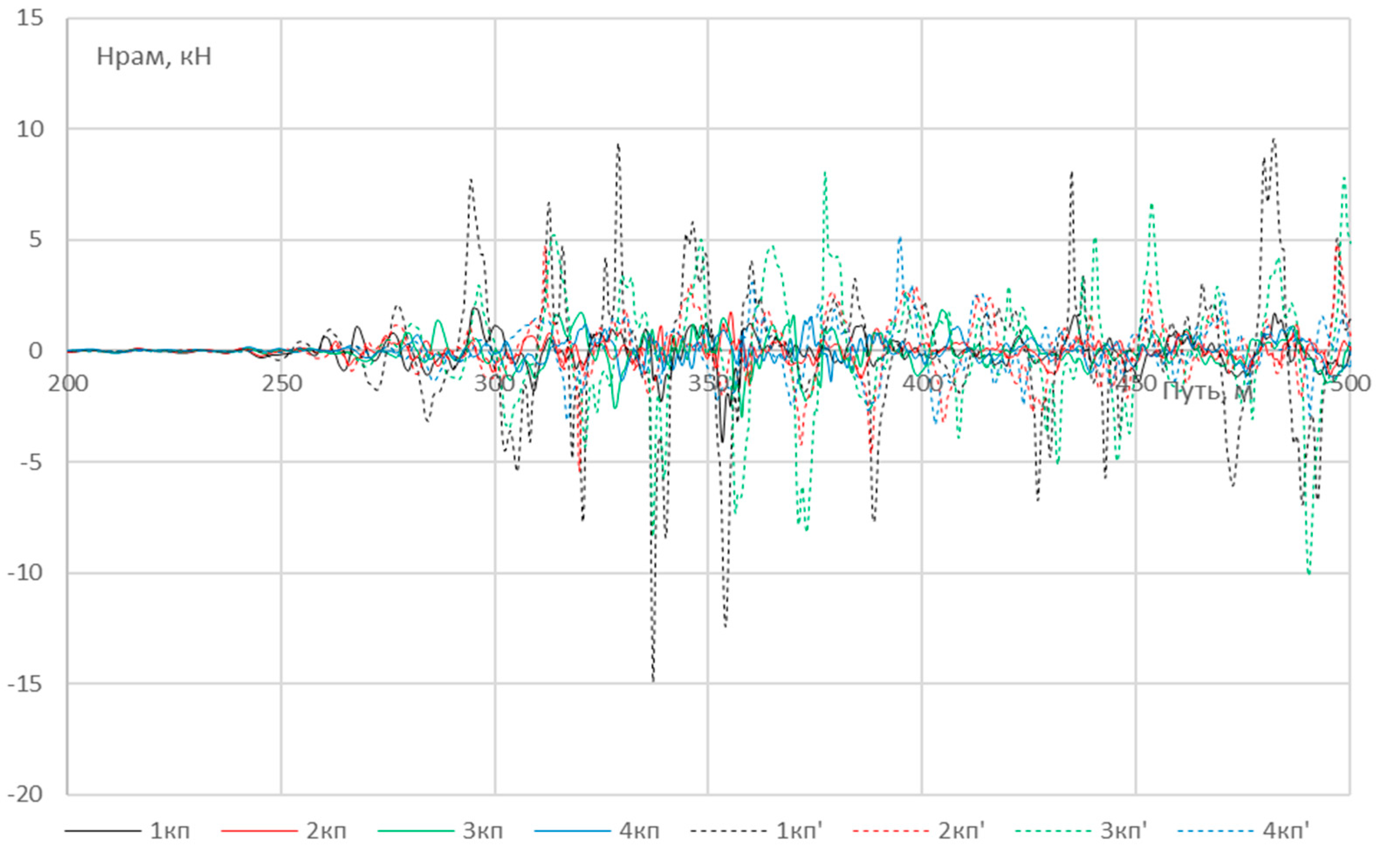
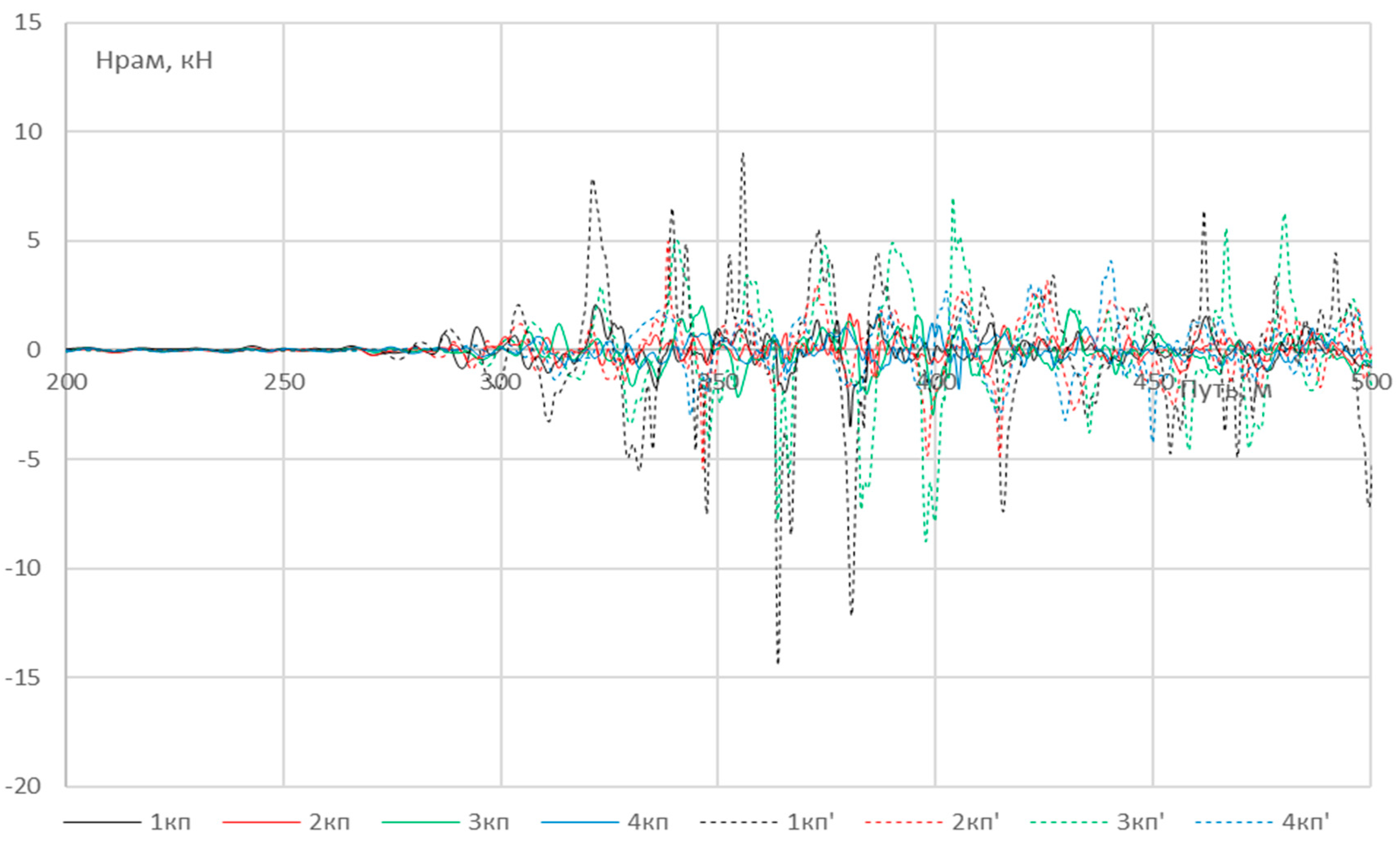
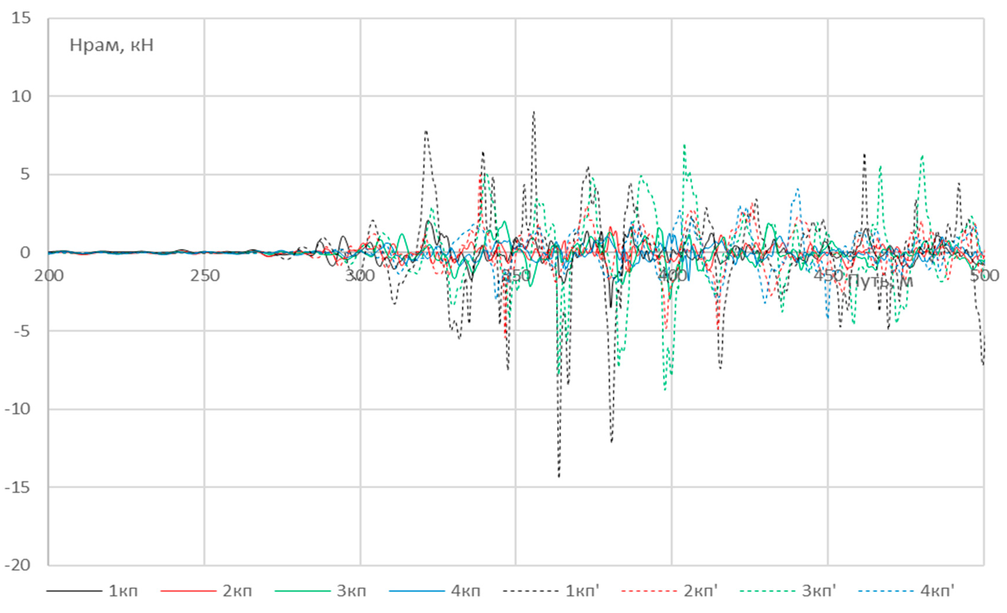
At the next stage, a comparative analysis of transverse oscillations was carried out, i.e. analysis of the frame forces of cars during the passage of a track section 500 m long in braking and coasting modes at a constant speed. From the oscillograms of the frame forces in the braking and coasting modes, it can be seen that the frame forces in the braking mode are lower than in the coasting mode (Figure 37, Figure 38, Figure 39 and Figure 40). In this case, the values with a dash correspond to the overrun mode [30]. This indicates that the derailment of the cars could not have occurred due to the shift of the rail and sleeper grid caused by an increase in the values of the transverse forces acting from the side of the wheels on the rails during braking, since in the rundown mode the frame forces, as a rule, have higher values.

The purpose of the next stage was to determine the influence of the shape of the unevenness on the behavior of the rolling stock. A series of numerical experiments were carried out for the movement of a single car [31]. When assessing the traffic safety of a single passenger car, due to the small effect on transverse vibrations, braking and longitudinal forces are not taken into account. The forms of irregularities shown in Figure 26 and Figure 27 are assumed to be the same for both threads without shifting relative to each other. The conditions for conducting numerical experiments are as close as possible to real ones [5]. The analysis was carried out in terms of the transverse displacement of the wheelset relative to the track axis, at which the derailment of the wheels becomes possible. Table 3 shows the conditions for conducting numerical experiments.

Table 4 and Table 5 show the roughness values at which wheels derailment is possible.

From the data given in Table 4 and Table 5, it can be seen that for a single unevenness of type 1, wheel derailment is possible at values a=95-100 mm, L=6 m, and for a double-sided unevenness of type 2 at a=80 mm, L= 6 m.

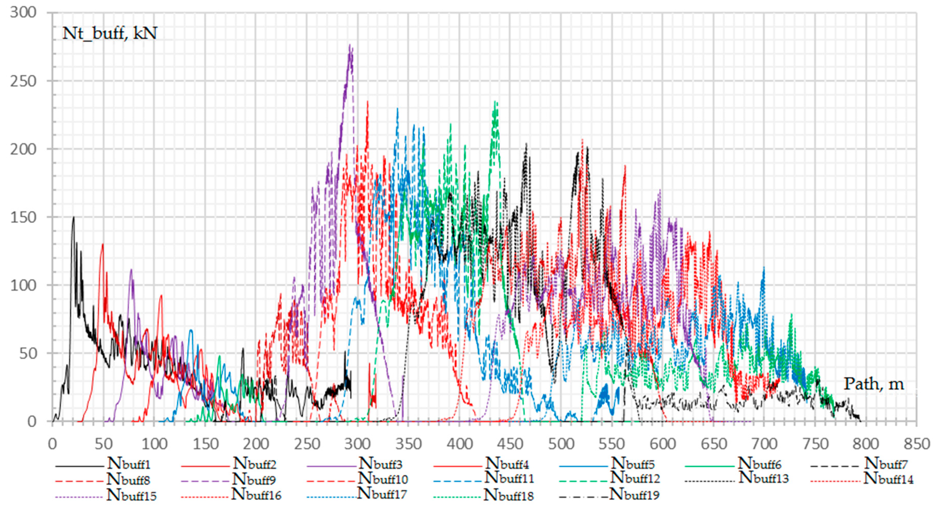
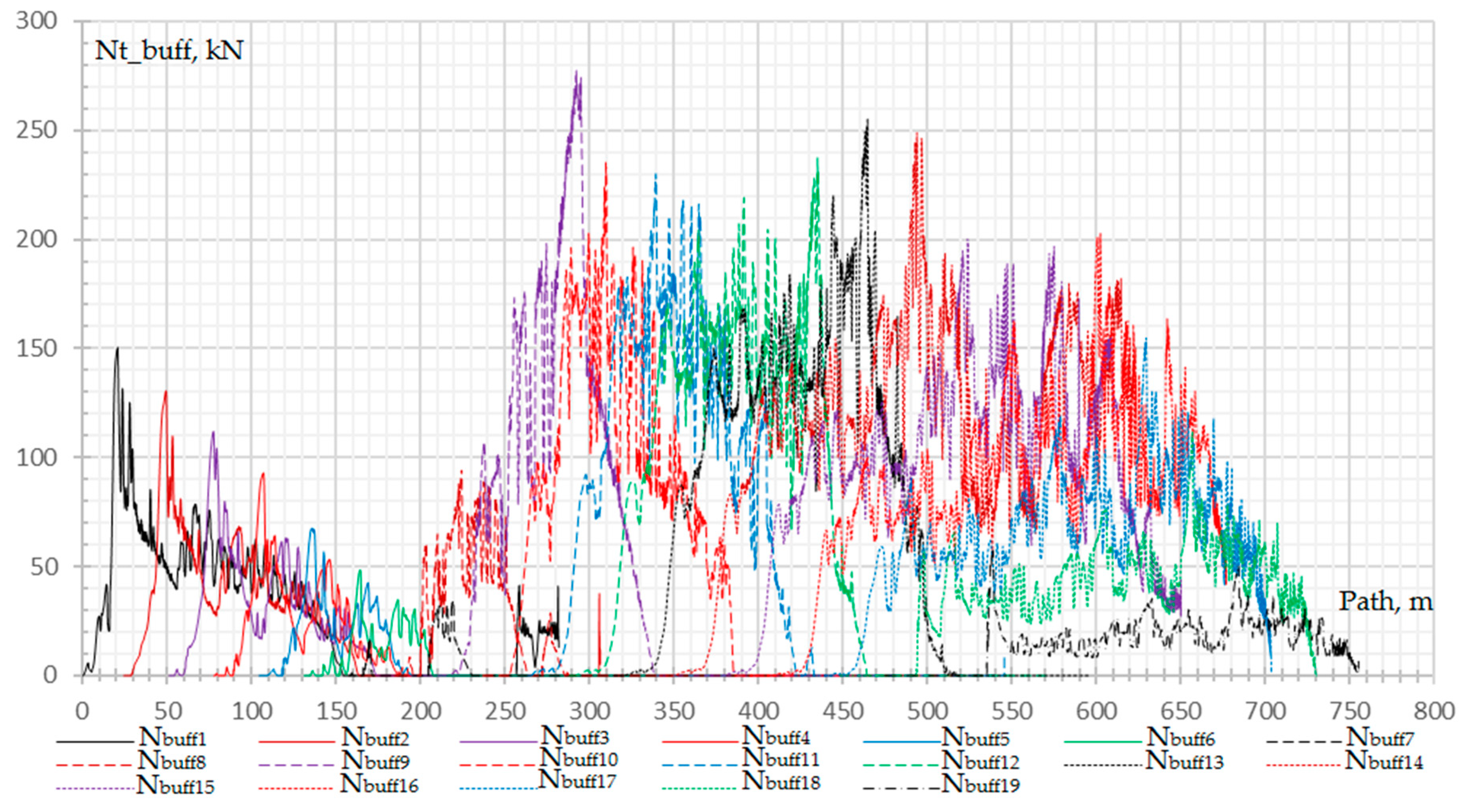
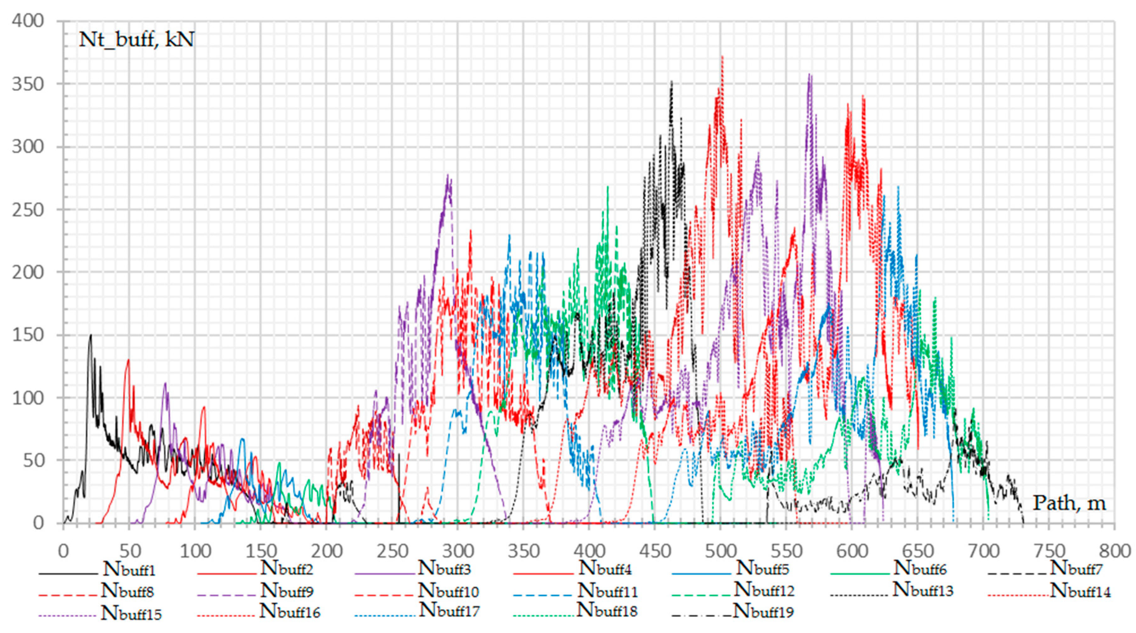
At the same time, the behavior of the car is noticeably different with the right and left irregularities [12]. An analysis of the longitudinal forces in the tail couplers and the total longitudinal forces of the tail couplers in the buffers of the locomotive and cars showed that the forces of additional resistance to the movement of the train, arising after the derailment of the wheels, contribute to the gradual emergence of tensile forces in the automatic couplers of the front cars [16]. With options No. 1 and No. 2, the longitudinal tensile effect does not reach the locomotive, and with option No. 3, the tensile effect reaches the locomotive 150 meters after the possible exit of car No. 8, which corresponds to the passage of cars No. 13-14 of the place of possible exit.

Figure 41. Longitudinal forces on the tail couplers of the locomotive and cars (option No. 1).

Figure 42. Longitudinal forces on the tail couplers of the locomotive and cars (option No. 2).

Figure 43. Longitudinal forces on the tail couplers of the locomotive and cars (option No. 3).

Figure 44. Total longitudinal forces on the tail buffers of cars (option No. 1).

Figure 45. Total longitudinal forces on the tail buffers of cars (option No. 2).

Figure 46. Total longitudinal forces on the tail buffers of cars (option No. 3).

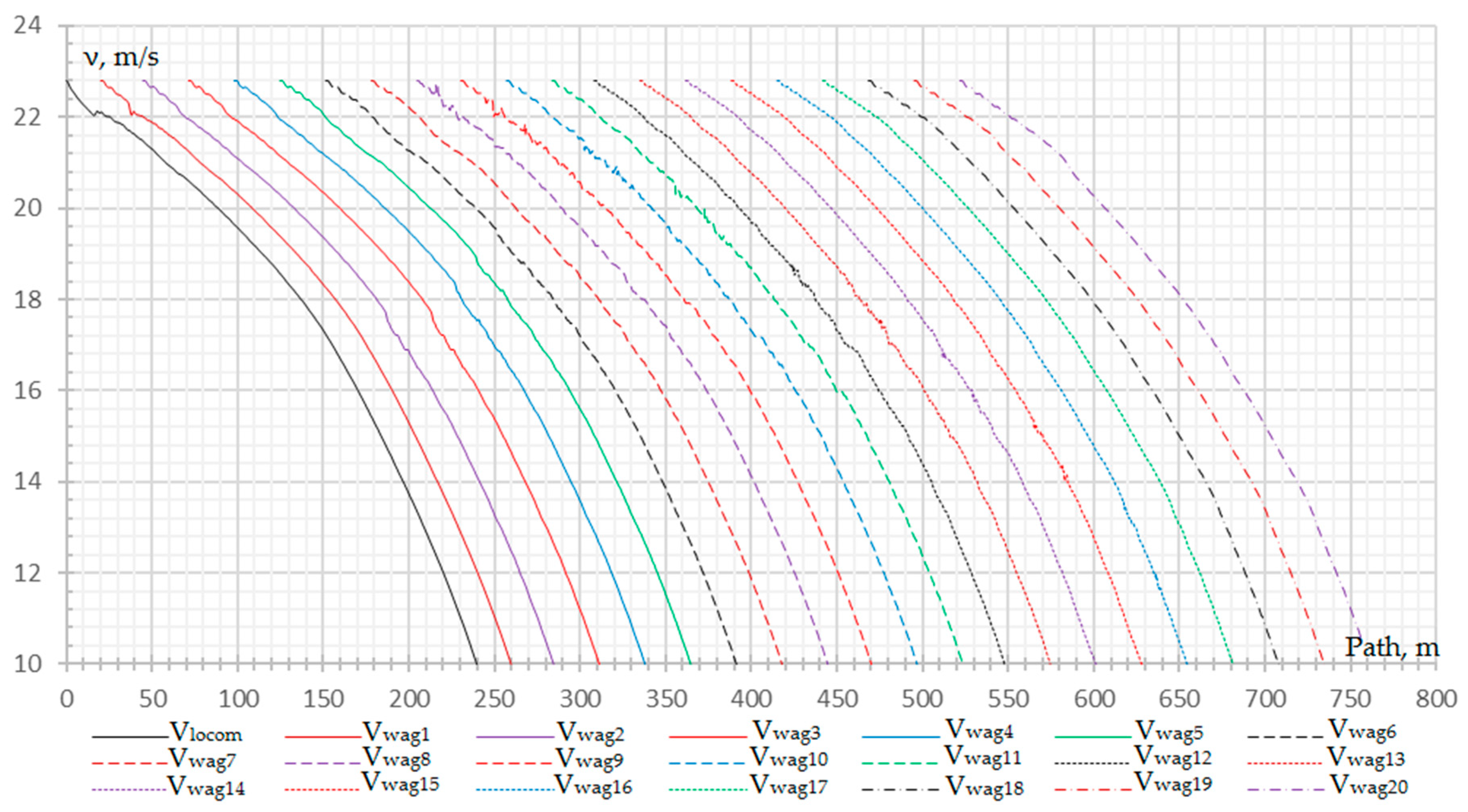
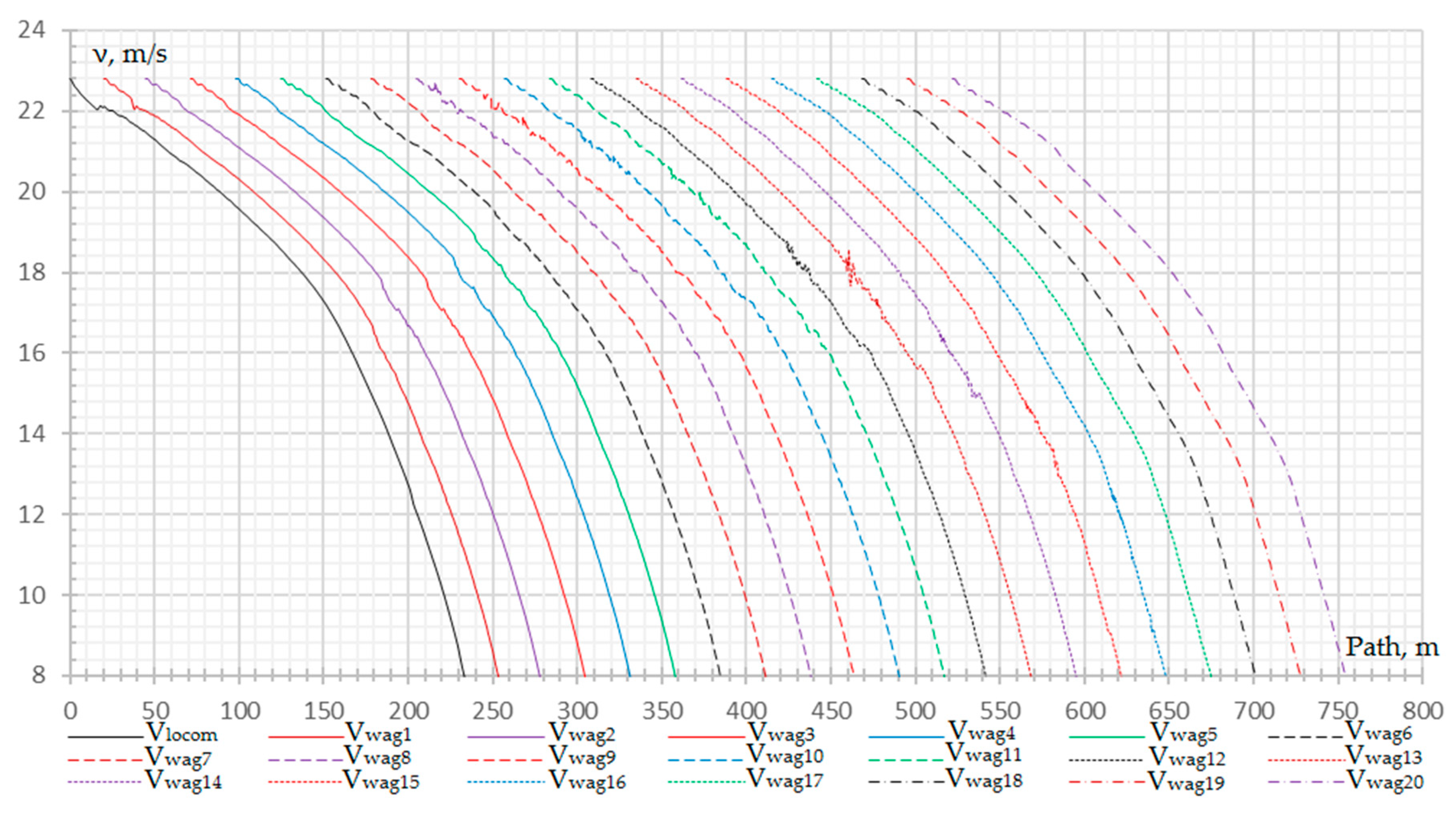
The first jumps of compressive and tensile forces in all three options under consideration correspond to the tail coupler and buffers of car No. 9, since after the possible derailment of the 3rd and 4th wheel sets of car No. 8 and all the wheel sets of car No. 9, the subsequent cars that have not yet come down run into and create a compressive force, while the front part moves at a speed slightly greater than this car and creates a tensile force. For clarity, let's consider the graphs for reducing the speeds of the locomotive and wagons (Figure 47, Figure 48, Figure 49 and Figure 50). 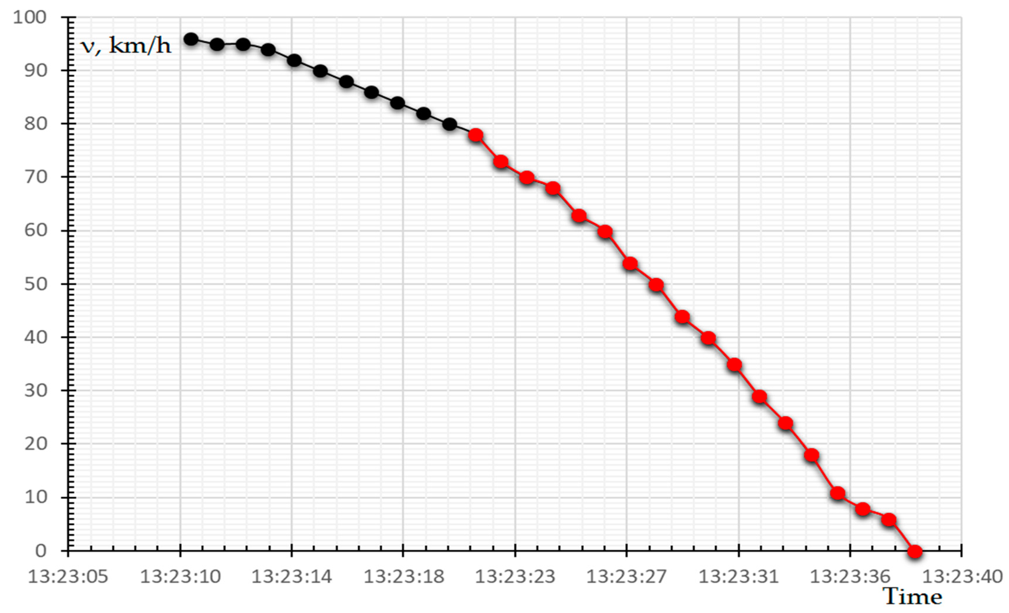From the graphs for reducing the speeds [17], it can be seen that with an increase in the forces of additional resistance to movement, jerks become more noticeable. This is especially noticeable in option No. 3, when cars No. 12 and 13 derail. Starting from the 12th second of the passenger train braking simulation, the linear (smooth steady) decrease in speed ends, and the zone of stepwise (unsteady) speed decrease begins (Figure 50).

4. Conclusions

This section is not mandatory but can be added to the manuscript if the discussion is unusually long or complex. Equations have been made that allow one to determine the linear and angular displacements, velocities and accelerations of the bodies included in the car model, as well as any points belonging to the bodies, when specifying their position in the coordinate system of the corresponding body.

To study the mode of emergency braking of a passenger train, a computational model of the longitudinal dynamics of the train is proposed, which is a chain of solid bodies connected by nonlinear links that take into account the state in each connection and its characteristics, including gaps.

The simulation modeling of the movement of a passenger train consisting of a locomotive and twenty passenger cars in the software environment "Universal Mechanism" in the emergency braking mode was performed.

On the example of the generated model, the calculated braking distance of the train was determined and the analysis of the longitudinal force between the automatic couplers of adjacent cars was carried out, in the state of the track with irregularities shown in Figure 20, Figure 21, Figure 22, Figure 23, Figure 24 and Figure 25.

As studies have shown, the use of emergency braking can cause derailment of passenger cars under certain circumstances discussed in this article.

Taking into account the conditions given in Table 4 and Table 5, it can be seen that for a single unevenness of type 1, wheel derailment is possible at values a=95-100 mm, L=6 m, and for a double-sided unevenness of type 2 at a=80 mm, L =6 m.

An analysis of the oscillograms of the total longitudinal forces between adjacent units of the rolling stock, depending on the distance traveled, showed that, due to the presence of buffer devices, braking is shockless, except for the connection between the locomotive and the first car.

The estimated braking distance was 583 m from the moment the emergency braking was applied, it should be noted that this value is within the limits of current standards and complies with regulatory and technical documents.

As studies have shown, the derailment of cars is not possible in the case of a shift of the rail-sleeper lattice caused by an increase in the magnitude of the transverse forces acting from the side of the wheels on the rails during braking. This is due to the fact that the frame forces obtained in the simulation have little effect on the track in the coastdown mode and, as a rule, have higher values in practice.

As the main recommendations, it should be noted the relevance of the development and implementation of automated systems for warning about a malfunction of the track in the direction of the train, about the presence of animals, people or vehicles on the railway track or railway crossing. Such developments can be created using a symbiosis of artificial intelligence, satellite navigation systems and emergency warning systems in "smart trains" equipped with computers of the required computing power.

Author Contributions

Conceptualisation, J.M.; methodology, J.M. and A.Z.; software, J.M.; validation, A.Z. and J.M.; formal analysis, A.Z. and J.M.; investigation, A.Z. and J.M.; resources, B.K. and S.Y.; data curation, G.S. and U.M.; writing—original draft preparation, S.Z.; writing—review and editing, A.Z. and J.M.; visualisation, J.M.; supervision, J.M. All authors have read and agreed to the published version of the manuscript.

Funding

This research received no external funding.

Institutional Review Board Statement

The study did not require ethical approval.

Informed Consent Statement

Not applicable.

Data Availability Statement

All data products generated in this study (velocity models, the performed studies) are available from the authors upon request.

Acknowledgements

This work was carried out in the research laboratory of the Institute of Civil Engineering of the Academy of Logistics and Transport, for which the authors are grateful.

Conflicts of Interest

The authors confirm that they have no conflict of interest with respect to the work described in this manuscript.

References

Musayev, J.; Abilkaiyr, Z.; Kaiym, T.; Alpeisov, A.; Alimbetov, A.; Zhauyt, A. The interaction of the freight car and way taking into account deformation of assembled rails and sleepers. Vibroeng. Procedia 2016, 8, 269–274. [Google Scholar]
Musayev, J.; Solonenko, V.; Mahmetova, N.; Kvashnin, M.; Zhauyt, A.; Buzauova, T. Modeling of dynamic characteristics of freight car with optimized parameters of wedge-type shock absorber. J. Vibroeng. 2017, 19, 1197–1213. [Google Scholar]
Günay, M.; Korkmaz, M.E.; Özmen, R. An investigation on braking systems used in railway vehicles. Eng. Sci. Technol. Int. J. 2020, 23, 421–431. [Google Scholar] [CrossRef]
Zhu, T.; Xiao, S.; Lei, C.; Wang, X.; Zhang, J.; Yang, B.; Yang, G.; Li, Y. Rail vehicle crashworthiness based on collision energy management: An overview. Int. J. Rail Transp. 2020, 9, 1–31. [Google Scholar] [CrossRef]
Liu, P.; Wang, K.; Zhang, D. Influence of Traction and Braking Operation on Wheel-Rail Dynamic Interaction for Heavy Haul Locomotive. China Railw. Sci. 2017, 38, 96–104. [Google Scholar]
Zakeri, J.A.; Xia, H. Sensitivity analysis of track parameters on train-track dynamic interaction. J. Mech. Sci. Technol. 2008, 22, 1299–1304. [Google Scholar] [CrossRef]
Wei, D.; Wei, X.; Jia, L. Automatic Defect Description of Railway Track Line Image Based on Dense Captioning. Sensors 2022, 22, 6419. [Google Scholar] [CrossRef]
Biži´c, M.B.; Petrovi´c, D.Z.; Tomi´c, M.C.; Djinovi´c, Z.V. Development of method for experimental determination of wheel–rail contact forces and contact point position by using instrumented wheelset. Meas. Sci. Technol. 2017, 28, 075902. [Google Scholar] [CrossRef]
Dumitriu, M.; Fologea, D.; Cruceanu, I.C. Effects analysis of vertical track irregularities on bogie vibration—Method based on bogie modelling and wheelsets accelerations measurement. IOP Conf. Ser. Mater. Sci. Eng. 2021, 1018, 012001. [Google Scholar] [CrossRef]
Gao, T.; Cong, J.; Wang, P.; Liu, J.; Wang, Y.; He, Q. Vertical track irregularity analysis of high-speed railways on simply-supported beam bridges based on the virtual track inspection method. Proc. Inst. Mech. Eng. Part. F J. Rail Rapid Transit. 2020, 235, 328–338. [Google Scholar] [CrossRef]
Li, H.; Yang, W.G.; Liu, P.; Wang, M. Prediction method and experimental verification of vibration response caused by underground high-speed railways. J. Low. Freq. Noise Vib. Act. Control 2022, 42, 452–469. [Google Scholar] [CrossRef]
Olivier, B.; Verlinden, O.; Kouroussis, G. Comparison of X–T and X–X co-simulation techniques applied on railway dynamics. Multibody Syst. Dyn. 2022, 55, 39–56. [Google Scholar] [CrossRef]
Bondarenko, I.; Keršys, R.; Neduzha, L. Analysis of Problem Related to Experimental Data Processing in the Study of the Rolling Stock Influence on the Track. In Proceedings of the 26th International Conference Transport Means, Kaunas, Lithuania, 5–7 October 2022; pp. 663–668. [Google Scholar]
Doi, H.; Hondo, T.; Nishiyama, Y.; Kuniyuki, S.; Tanaka, T. Stationary Test Method for Evaluating Wheel Unloading of Railway Vehicle on Twisted Track Simulated with Spacers between Wheel and Rail. Proc. Transp. Logist. Conf. 2020, 29, 3801. [Google Scholar] [CrossRef]
Wang, H.; Berkers, J.; Hurk, N.V.D.; Layegh, N.F. Study of loaded versus unloaded measurements in railway track inspection. Measurement 2020, 169, 108556. [Google Scholar] [CrossRef]
De Souza, E.F.; Bittencourt, T.N.; Ribeiro, D.; Carvalho, H. Feasibility of Applying Mel-Frequency Cepstral Coefficients in a Drive-by Damage Detection Methodology for High-Speed Railway Bridges. Sustainability 2022, 14, 13290. [Google Scholar] [CrossRef]
17. DSTU 7571:2014, K: Stock Permissible Exposure Norms to the Railway Track Width 1520 mm. Minekonomrozvitku, 1520.
Spiroiu, M.A.; Nicolescu, M. On the estimation of the reliability probabilistic model of railway wheelset. IOP Conf. Ser. Mater. Sci. Eng. 2019, 682, 012001. [Google Scholar] [CrossRef]
Wang, K.; Huang, C.; Zhai, W.; Liu, P.; Wang, S. Progress on wheel-rail dynamic performance of railway curve negotiation. J. Traffic Transp. Eng. 2014, 3, 209–220. [Google Scholar] [CrossRef]
Ahmed, K.W.; Sankar, S. Steady-State Curving Perform. Railw. Freight. Truck. Damper-Coupled Wbeelsets. Veh. Syst. Dyn. 1988, 26, 295–315. [Google Scholar] [CrossRef]
Cherkashin, Y.M.; Pogorelov, D.Y.; Simonov, V. A. Influ. Roll. Stock. Track. Parameters Train. Traffic Saf. Vestn. VNIIZhT 2010, 2, 11–20. [Google Scholar]
Chi, M.R.; Wang, K.W.; Fu, M.H.; et al. Study on curving performance for bogie with magnetic fluid coupled wheel-sets. J. China Railw. Soc. 2002, 24, 28–33. [Google Scholar]
Dukkipati, R.V.; Swamy, S.N. Lateral stability and steady state curving performance of unconvertional rail truck. Mech. Mach. Theory 2001, 36, 577–587. [Google Scholar] [CrossRef]
Gialieonaido, E.D.; Braghin, F.; Biuni, S. The influence of track modeling options on the simulation of rail vehicle dynamics. J. Sound. Vib. 2012, 331, 4246–4258. [Google Scholar]
Huang, Y.H.; Li, F.; Fu, M.H. Res. Curving Perform. A Bogie Indep. Rotating Wheel. China Railw. Sci. 2001, 22, 7–11. [Google Scholar]
Kurzeck, B. Combined friction induced oscillations of wheelset and track during the curving of metres and their influence on corrugation. Wear 2011, 271, 299–310. [Google Scholar] [CrossRef]
Lee, S.Y.; Cheng, Y.C. Influences of the vertical and the roll motions of frames on the hunting stability of trucks moving on curved tracks. J. Sound. Vib. 2006, 294, 441–453. [Google Scholar] [CrossRef]
Lu, Z.G.; Zhao, H.X. Curve performance study and parameter design of flexible coupled single-wheelset running gears. China Railw. Sci. 2004, 25, 32–37. [Google Scholar]
Ni, P.T.; Wang, K.W.; Chen, J.; et al. Influence of anti-hunting damper on critical velocity and high-speed curve negotiating performance of the vehicle with MRF coupled wheelsets. J. China Railw. Soc. 2007, 29, 34–39. [Google Scholar]
Ren, Z.S.; Sun, S.G. Study on the influence of parameters to the dynamics of light rail vehicles with independently rotating wheel. Electr. Locomot. Mass. Transit. Veh. 2003, 26, 22–24. [Google Scholar]
Bondarenko, I.; Lukoševičius, V.; Keršys, R.; Neduzha, L. Investigation of Dynamic Processes of Rolling Stock–Track Interaction: Experimental Realization. Sustainability 2023, 15, 5356. [Google Scholar] [CrossRef]

Figure 1. General view of the locomotive model.

Figure 2. General view of the passenger car model.

Figure 3. Point-to-plane contact interaction.

Figure 4. Design schemes of rheological models.

Figure 5. Rail position in transverse direction.

Figure 6. Scheme of contact interaction of wheels and the surface of the earth.

Figure 7. Scheme of contact interaction of wheels and rails in cross-sliding.

Figure 11. Indicator diagram of the filling of the brake cylinder of a passenger car during emergency braking with an electro-pneumatic brake.

Figure 12. Indicator diagram of brake pressure on the block of a passenger car.

Figure 14. Diagram of the total brake pressure on the axle of the locomotive.

Figure 17. The main specific resistance to the movement of the locomotive.

Figure 18. The main specific resistance to the movement of the car (in terms of Newton’s).

Figure 19. The main specific resistance to the movement of the car (in terms of Newton’s).

Figure 22. Irregularities of the right rail thread 1-2 wheel pair (WP).

Figure 23. Irregularities of the left rail thread 1-2 wheel pair (WP).

Figure 26. Fading roughness

η (t) = a ∙ c o s (2 ∙ π ∙ \frac{x}{L}) ∙ \frac{1}{1 + b ∙ x^{2}}

Figure 26. Fading roughness

η (t) = a ∙ c o s (2 ∙ π ∙ \frac{x}{L}) ∙ \frac{1}{1 + b ∙ x^{2}}

Figure 27. Fading roughness

η (t) = a ∙ s i n (2 ∙ π ∙ \frac{x}{L})

Figure 27. Fading roughness

η (t) = a ∙ s i n (2 ∙ π ∙ \frac{x}{L})

Figure 28. General view of the train model.

Figure 29. Graph of the decrease in the speeds of the rolling stock units of the train during braking.

Figure 30. Graph of deceleration of train rolling stock units (transient process).

Figure 31. Oscillograms of longitudinal forces on the tail couplers of the locomotive and wagons.

Figure 32. Oscillograms of longitudinal forces on the tail couplers of the locomotive and cars No. 1-3.

Figure 33. Oscillograms of longitudinal forces on the tail couplers of cars No. 4-7.

Figure 34. Oscillograms of longitudinal forces on the tail couplers of cars No. 8-11.

Figure 35. Oscillograms of longitudinal forces on the tail couplers of cars No. 12-15.

Figure 36. Oscillograms of longitudinal forces on the tail couplers of cars No. 16-19.

Figure 37. Oscillograms of the frame forces of the wheel pairs (wp) of the 8th car (dashed values correspond to coast down mode).

Figure 38. Oscillograms of the frame forces of the wheel pairs (wp) of the 9th car (dashed values correspond to coast down mode).

Figure 39. Oscillograms of the frame forces of the wheel pairs (wp) of the 10th car (dashed values correspond to coast down mode).

Figure 40. Oscillograms of the frame forces of the wheel pairs (wp) of the 11th car (dashed values correspond to coast down mode).

Figure 47. Graph of the speed reduction of the locomotive and wagons (option No. 1).

Figure 48. Graph of the speed reduction of the locomotive and wagons (option No. 2).

Figure 49. Graph of the speed reduction of the locomotive and wagons (option No. 3).

Figure 50. Graph of deceleration during deceleration.

Table 1. Permissible values of the estimated indicators.

Index		Standard values
Ratio of frame force to static axial load H_P/P₀	Excellent	≤0.20
	Good	0.25
	Satisfactory	0.30
	Permissible	0.38
Lateral forces, kN	Permissible	100
Wheel stability factor against derailment λ_normal	in direct	1.3

Table 2. Technical characteristics of the rolling stock (accepted for modeling).

Serial number in the train	Container, ton	Length along the clutch axes, m	Base, m	Additional weight from passengers and cargo, ton	Gross weight, ton
Locomotive		20.032	10.3		85
wagon №1	55	24.537	17	3.5	58.5
wagon №2-7, 10, 12	61.5	26.696	19	4	65.5
wagon №8	58.1	25.5	17	3.5	61.6
wagon №9	61.5	26.696	19	3.5	65
wagon №11	61	24.537	17	0.5	61.5
wagon №13-19	60	26.696	19	6	66
wagon №20	51	24.537	17	6	57

Table 3. Conditions for carrying out numerical experiments.

№	Name	Meaning	Unit
1	Path microgeometry	Straight	-
2	Vertical stiffness per rail	50	МN/m
3	Transverse stiffness per rail	20	MN/m
4	Vertical dissipation per rail	800	kN/m
5	Transverse dissipation per one rail thread	320	kN/m
6	Rail profile	New Р65
7	Wagon wheel profile	New
8	Modulus of elasticity in wheel-rail contact	210*10⁹
9	Poisson's ratio in wheel-rail contact	0,27
10	Coefficient of friction between wheel and rail	0,25
11	Travel speed	96	km/h
12	Wagon base	19	m
13	Wagon gross weight	65,5	ton
14	The distance between the extrema of two small waves of irregularity of type 1	6; 9; 14	m
15	The distance between the extrema of two adjacent waves of irregularity of type 2	6; 12; 18	m

Table 4. Descent matrix for roughness type 1.

а, mm	l, m
	1 WP			2 WP			3 WP			4 WP
	6	9	14	6	9	14	6	9	14	6	9	14
left roughness
<95
100
105-115
120<
right roughness
<90
95
100
105-120
125<

Table 5. Descent matrix for roughness type 2.

а, mm	l, m
	1 WP			2 WP			3 WP			4 WP
	6	12	18	6	12	18	6	12	18	6	12	18
left roughness
75
80-160
165-280
285
290
right roughness
<75
80-155
160-275
280<

Disclaimer/Publisher’s Note: The statements, opinions and data contained in all publications are solely those of the individual author(s) and contributor(s) and not of MDPI and/or the editor(s). MDPI and/or the editor(s) disclaim responsibility for any injury to people or property resulting from any ideas, methods, instructions or products referred to in the content.

© 2023 by the authors. Licensee MDPI, Basel, Switzerland. This article is an open access article distributed under the terms and conditions of the Creative Commons Attribution (CC BY) license (http://creativecommons.org/licenses/by/4.0/).

Copyright: This open access article is published under a Creative Commons CC BY 4.0 license, which permit the free download, distribution, and reuse, provided that the author and preprint are cited in any reuse.

Alerts

MDPI Initiatives

Important Links

Choose an area of interest and we will send you notifications of new preprints at your preferred frequency.

Disclaimer

Modeling the Interaction of the Rolling Stock and the Track in the Emergency Braking Mode of a Passenger Train

Abstract

Keywords:

Subject:

1. Introduction

2. Materials and Methods

3. Results (Motion Simulation)

4. Conclusions

Author Contributions

Funding

Institutional Review Board Statement

Informed Consent Statement

Data Availability Statement

Acknowledgements

Conflicts of Interest

References

MDPI Initiatives

Important Links

Subscribe