1. Introduction
Madre de Dios (MDD) is an important rainforest region located in the southeastern Peruvian Amazonian, recognized for its biological and cultural diversity [1-3], and an important biomass stock reserve [
4]. Over the last 40 years this region has been threatened by illegal alluvial gold mining. This activity involves deforestation, soil excavation and use of liquid mercury [
5] causing permanent loss of the ecosystem, severe soil erosion, water pollution, mercury in hydrobiology and human health problems [6-10]. Between 1984 and 2017, 100,000 ha of accumulated deforestation due to alluvial gold mining activities have been identified [
11]. Deforestation increases soil erosion and surface runoff rates, leading to increased sedimentation rates and alteration of the hydrological cycle [
12], removing cover vegetation also increases soil compaction and reduces infiltration capacities, leading to floods [
13] which are frequent in the wet seasons, especially in mining zones of the MDD basin.
Soil and Water Assessment Tool (SWAT) is a watershed-scale model widely used to determine hydrologic responses resulting from changes in land use and land cover [
14]. The SWAT model has been successfully implemented in multiple geographical regions worldwide to understand how alterations in land use and land cover can influence local hydrology and sediment yields. Significant findings from these studies in the Brazilian Amazonia, include the observation of increasing trends in surface runoff and sediment yield, with a simultaneous decrease in evapotranspiration [
15]. Additionally these studies have revealed increased flow during the high-flow season and decreased flow during the low-flow season, leading to the intensification of extreme flow events [
16]. The impact of alterations in land use and land cover on hydrology and sediment yields may not be uniform across different geographical regions, uppermost reaches of forested highlands were most significantly affected in an East African Watershed [
17], while the change in land use from forest to bare soil would increase the runoff-generating capacity in the Brazilian amazon much more than if it would be replaced by crop or pasture [
15].
Even though many interdisciplinary studies have been conducted to assess the impacts of alluvial gold mining in MDD, there is a knowledge gap where hydrological impacts due to deforestation remain unknown, mainly due to the lack of meteorological and hydrological available data. Precipitation data is an essential input to properly represent hydrological processes in hydrological models [
18]. Furthermore, it is considered as the first source of uncertainty [
19]. Due to the scarce availability of meteorological data measured in the Amazon Basin, several studies have been using satellite precipitation data, such as TRMM (Tropical Rainfall Measuring Mission) [
20], GMP (Global Precipitation Measurement) [
21] and CHIRPS (Climate Hazards Group Infrared Precipitation with Stations) [
22], as input for hydrological models [23-25].
This study is the first hydrological modeling application in MDD. Its main aim is assessing the effects of deforestation due to gold mining on the hydrological response and providing reliable streamflow daily data in main rivers leading to further studies. This study incorporates the CHIRPS product for precipitation [
22] and the CPC Global Unified Temperature provided by NOAA (National Oceanic and Atmospheric Administration) for temperature [
26]. The specific objective is to analyze the impact on hydrological variables, such as streamflow regime and surface runoff, on a future deforestation scenario in one of the most affected by deforestation and mining watersheds in the Peruvian Amazonia.
2. Materials and Methods
2.1. Study Area
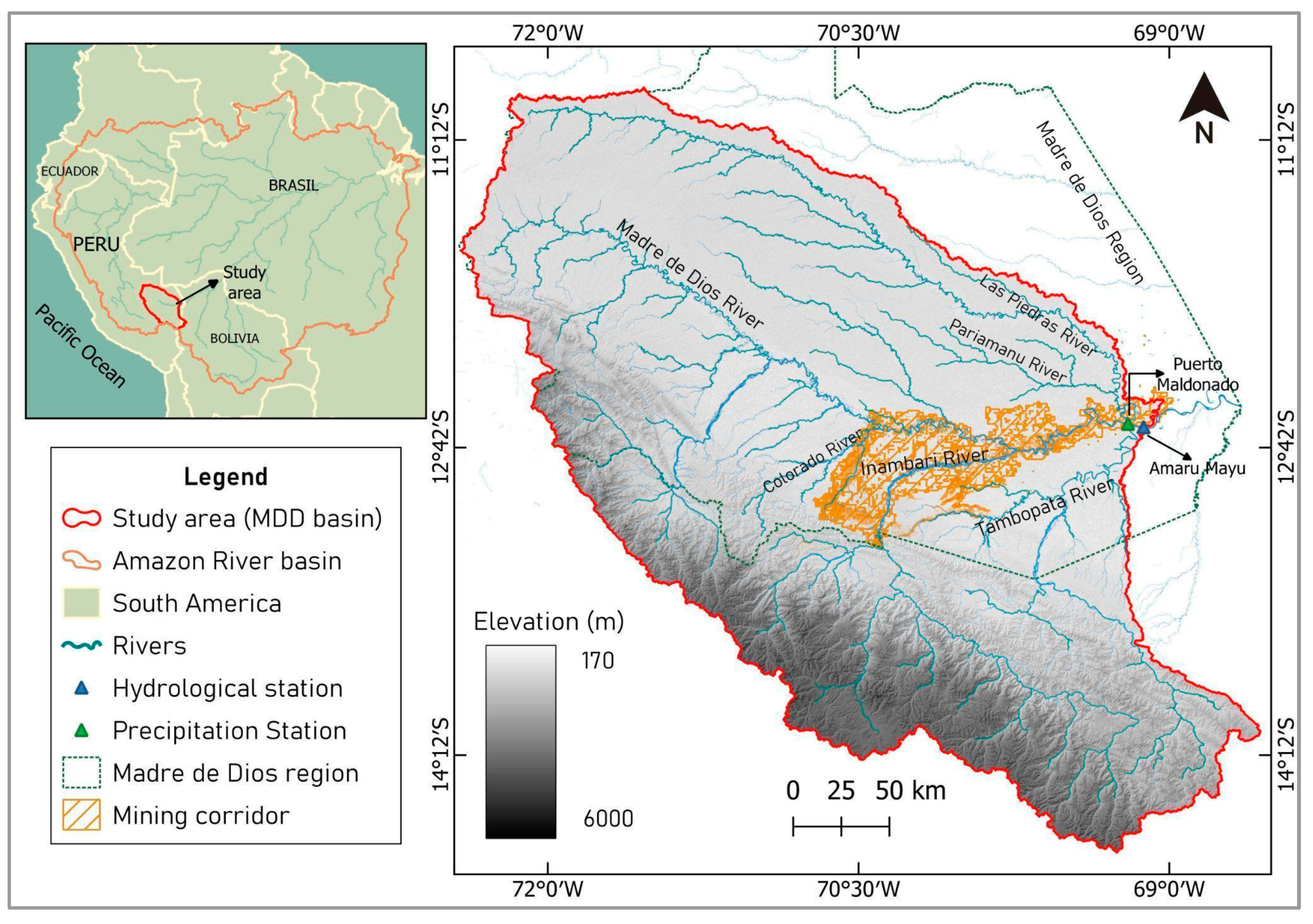
The Madre de Dios (MDD) basin (
Figure 1) is delimited from the Andes mountains until the outlet point Amaru Mayu located in the Madre de Dios River after the confluence of Tambopata River. This basin covers a drainage area of 90,750 km² (9,075 kha) with an elevation range between 170 and 6,000 m. The majority of the MDD basin predominantly consists of Southwest Amazon moist forests with a flat topography, characterized by floodplains exhibiting slopes of less than 5%. However, the basin area formed by the Andes Mountains or Peruvian Yungas displays notably steep slopes, with values exceeding 50%, finally the northwestern area comprises elevated uplands with slopes measuring less than 20%.
The MDD basin presents a warm, rainy to very rainy climate (more than 2,000 mm/year) throughout the year. The part of the study area bordering the Eastern Cordillera of the Andes is characterized by a highly rainy zone (6,000 mm/year on average) [
27]. According to the analysis of the monthly average of measurements from the Puerto Maldonado meteorological station (
Figure 1), the maximum precipitation of 384 mm/month occurs in December. The dry months cover the period from May to September, with a minimum precipitation of 32 mm/month in August and the average precipitation is 2,240 mm/year. The average annual minimum and maximum temperatures are 21.9°C and 31.3°C, respectively (
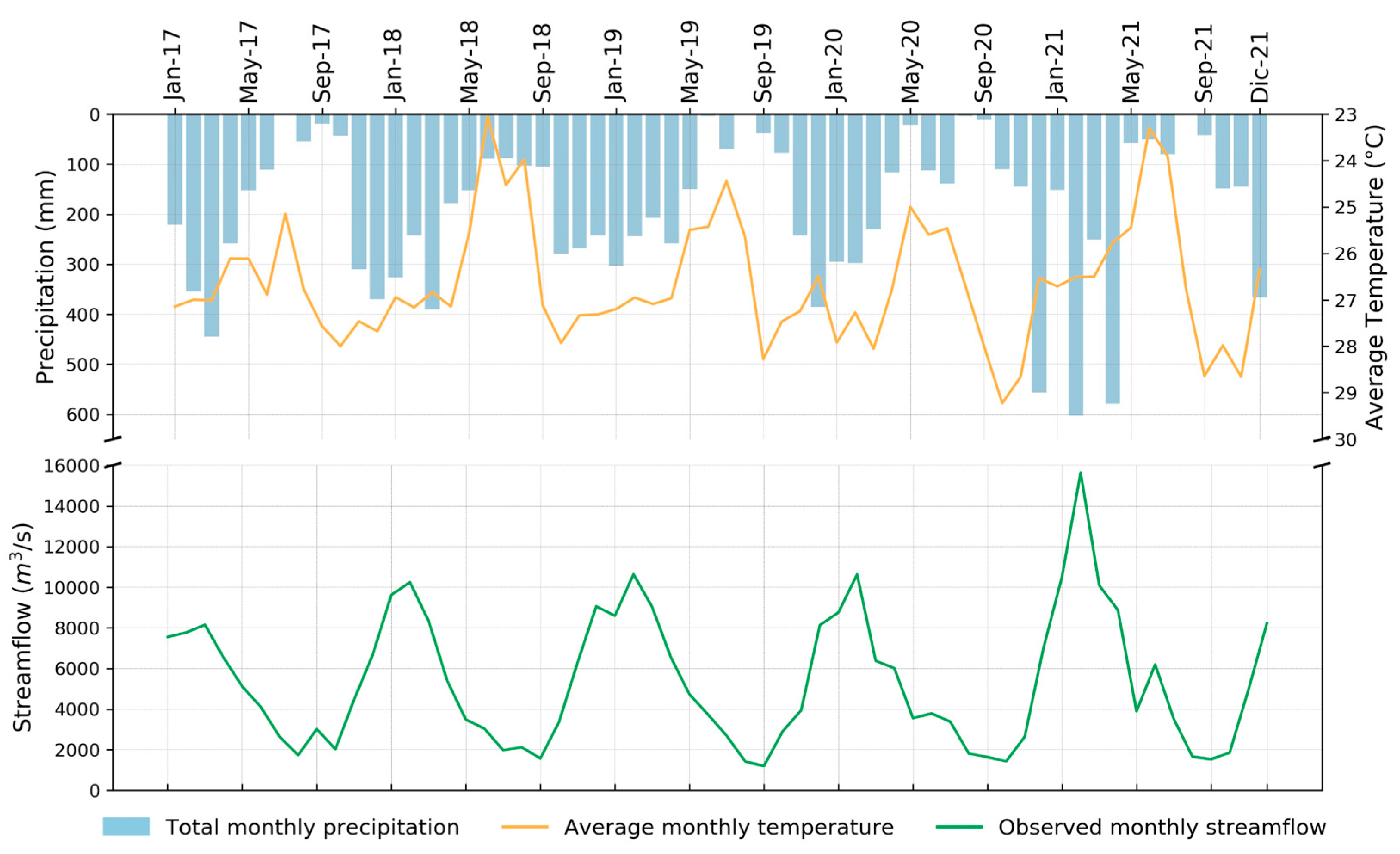
Figure 2).
Despite the delimited protected areas in the MDD region, this is one of the most severe examples of deforestation caused by gold mining in the entire Amazon [
28]. Based on the Global Forest Watch maps of tree cover loss from the Global Land Analysis and Discovery (GLAD) [
29] made available by the World Research Institute (WRI), a total area of 2,750 km² (equivalent to 275 kha) was deforested in the MDD region between 2001 and 2022. Similarly, the Peruvian Ministry of Environment (MINAM) has determined a significant forest loss of 2,097 km² (209 kha) within the Madre de Dios region between the years 2001 and 2018 [
30].
Even when agriculture concentrates the largest deforestation, mining deforestation has the potential to significantly impact critical areas such as river banks, protected areas and indigenous territories. Deforestation is most intense along the mining corridor (
Figure 1), this zone crosses along the Madre de Dios River and its floodplain including Colorado and Inambari Rivers.
2.2. Climate Data.
The study area's limited number of precipitation stations led to the evaluation of several gridded datasets. The SWAT model was executed utilizing the CHIRPS [
22], TRMM [
20], and PISCO [
31] daily precipitation datasets, followed by a comparison of the resultant streamflow outputs against the observed streamflow measurements obtained from the Amaru Mayu station (
Figure 1). The results were analyzed utilizing the statistical metrics outlined in equations 2, 3, and 4. The dataset demonstrating the highest degree of accuracy was subsequently identified and selected. Daily averaged grids for the period 1981–2021 have been calculated for each subbasin, since SWAT uses the nearest station to the centroid of each subbasin.
Daily maximum and minimum temperature data were obtained from CPC Global Unified Temperature, provided by the NOAA PSL [
25]. In this study 217 and 110 grids were used for precipitation and temperature, respectively over the period 1995-2021.
Streamflow data were collected from the hydrological station Amaru Mayu, located in the outlet point of the MDD basin (
Figure 1). The data was provided by the National Authority of Water of Peru (Autoridad Nacional del Agua - ANA) [
32]. The period available is from 2017 to the present. Average annual streamflow is 5,180 m
3. s
-1 , the average flow during the dry season (May to September) is 2,886 m
3. s
-1 while in the wet season (October to April) is 6,819 m
3. s
-1 Figure 2.
2.3. Topography, soil, and land use data.
The Digital Elevation Model (DEM) utilized in this study originates from the Shuttle Radar Topography Mission (SRTM) and possesses a spatial resolution of 30 meters [
33]: this information is necessary to delineate the basin, sub-basins and streamflow network. Furthermore, the model requires information about the types of soil and their physical properties such as texture, water holding capacity, hydraulic conductivity, and others. The soil type map (
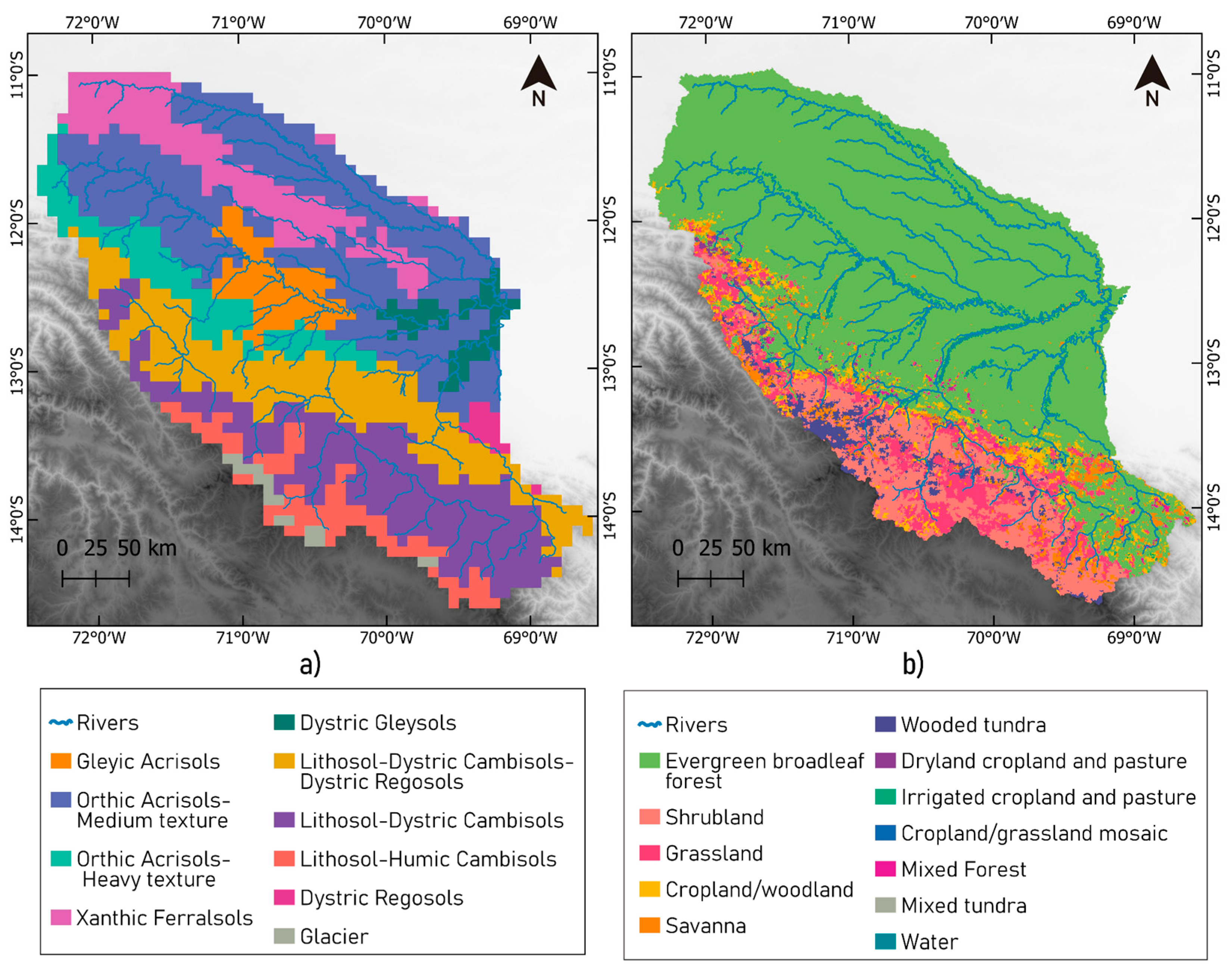
Figure 3a) was obtained from the Digital Soil Map of the World provided by the Food and Agriculture Organization of the United Nations (FAO) [
34]. In the MDD basin the soil types are Orthic Acrisols - Medium texture (30%); Lithosol-Dystric Cambisols (18%); Lithosol - Dystric Cambisols -Dystric Regosols (17%); Xanthic Ferralsols (11%); Orthic Acrisols - Heavy texture (8%); Lithosol-Humic Cambisols (6%); Gleyic Acrisols (5%); Dystric Gleysols (3%); and Glacier and Dystric Regosols less than 1% covering area. The land use cover map used to set up the preliminary SWAT model was from Global Land Cover Characterization (GLCC)- USGS [
35]. The map shown in
Figure 3b illustrates that the predominant land cover category, comprising 70%, is characterized by Evergreen Broadleaf Forest. Followed by Shrubland at a distant proportion of 9%, with Grassland occupying 8%, Cropland/Woodland Mosaic encompassing 4%, Savanna and Wooded Tundra each occupying 4% and 3% respectively, while other categories collectively represent less than 1%. Information related to the datasets presented above are summarized in
Table 1.
2.4. SWAT Model
The Soil and Water Assessment Tool (SWAT) is a process-based model designed for continuous-time simulation, featuring a semi-distributed structure. It is particularly suited for the representation of long-term basin-scale processes [
36]. SWAT stands out as a versatile and robust tool, capable of simulating diverse watershed scenarios across varying scales and environmental contexts worldwide [
37]. The model performs simulations dividing each basin into sub-basins. Every sub-basin is further subdivided into Hydrologic Response Units (HRUs). Every HRUs is a unique combination of land-use, soil, and slope in each sub-basin; this is why this model is called semi-distributed [
38]. In this study, the MDD basin was divided into 217 sub-basins and a total of 1244 HRUs. The water balance in SWAT is given by the Equation (1)
where SW
t is the final soil water content on day t (mm); SW
0 is the initial soil water content on day i (mm); t is time (d); R
day i is the precipitation depth on day i (mm); Q
sur if is the surface runoff volume on day i (mm); E
a i is the evapotranspiration depth on day i (mm); w
seep i is the amount of water entering the vadose zone from the soil profile on day i; and Q
gw i is the amount of return flow on day i.
2.4.1. Model setup
In this study, we utilized SWAT version 2012 (SWAT.v.2012) by means of the QSWAT 1.3 plug-in within the open-source Geographic Information System, QuantumGIS (QGIS) [
39].
The initial stage of the model, known as the warm-up period, is utilized to enable the hydrological model to operate for a significant duration before the simulation period begins. This allows important processes to reach a state of dynamic equilibrium. To achieve this, model developers suggest implementing warm-up periods lasting two to four years for watershed scale processes [
40]. Consequently, in this study, the time period between 1981 and 1984 was utilized as the warm-up period to ensure an appropriate initialization of the system. The simulation period covers 4 decades from 1985 to 2021, during which the model performed its operational simulations and generated results. As for the calibration period, it was restricted to the years 2016 to 2021, primarily driven by data availability. During this period, the model's parameters were adjusted to achieve the best possible fit with observed streamflow data.
The assessment of the model's performance consisted of a thorough examination, specifically comparing the observed and simulated streamflow data, focusing on sub basin number 215, which corresponds to the Amaru Mayu hydrological station during the period from 2016 to 2021.The validation process utilized the metrics outlined in
Table 2 [
41]. These metrics included the Nash-Sutcliffe coefficient of efficiency (NS) [
42], calculated using Equation 2, the percent bias (PBIAS) [
43] determined through Equation 3, and the root mean square error (RMSE)-observations standard deviation ratio (RSR) [
41] as derived from Equation 4.
where Q
i is the observed streamflow on day i, Q
ic is the simulated streamflow on a day i and
is the mean observed streamflow.
2.4.2. Deforestation scenario
The land use map allows the model to simulate and integrate responses of various cover types, and enables modelers to study land use cover change impacts by varying its spatial and temporal distribution [
44].
The "National Forest Conservation Program for Climate Change Mitigation" is under the management of the Peruvian Ministry of Environment (MINAM), using data from the Landsat 7 and 8 satellites, MINAM has established a methodology to identify early warning alerts for loss of humid tropical forest cover in Peru. These alerts, which are accessible via the Geobosques platform (
http://geobosques.minam.gob.pe) shows that among Peruvian regions, Madre de Dios consistently registers the highest density of these alerts annually, surpassing other areas [
45].
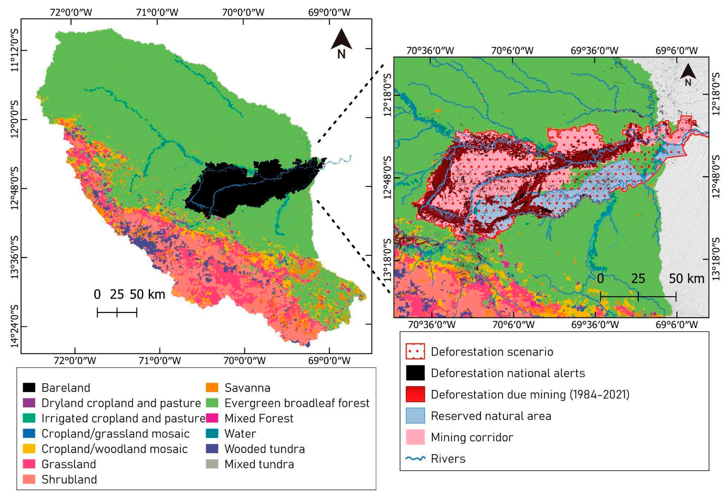
Figure 4 shows deforestation national alerts density inside the mining corridor and even inside the buffer zone of The National Tambopata Reserve (in blue color). In order to assess the impact of future deforestation in hydrologic variables, a future scenario of 8,109 km
2 (equivalent to 9% of the study area) was proposed. Within this scenario the land use was modified from evergreen broadleaf forest (FOEB) to bare land (BARE).
3. Results
3.1. Correlation between stream flows generated by CHIRPS, TRMM and PISCO precipitation datasets and in-situ data.
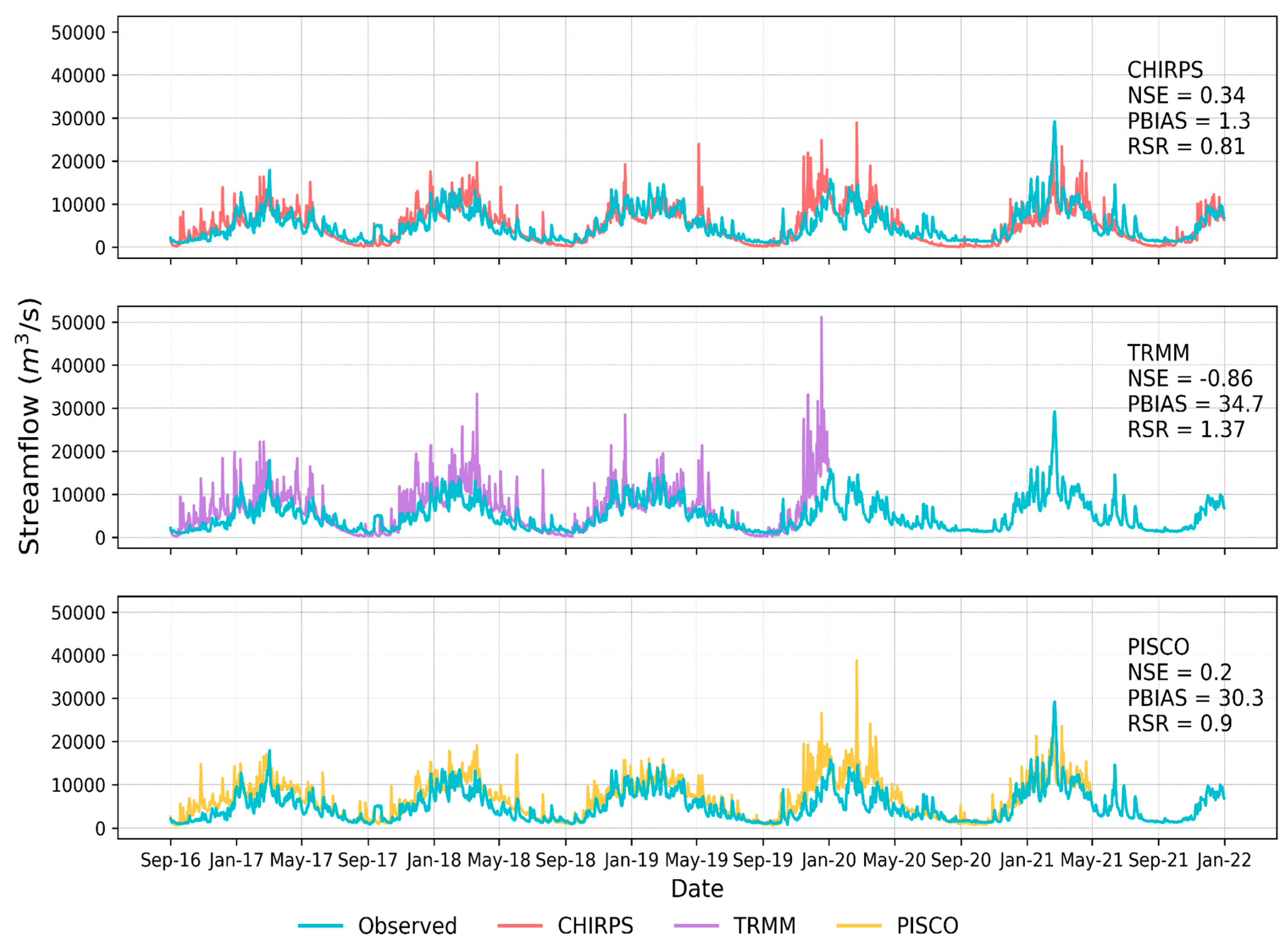
It is notable that the SWAT model was successful in simulating the seasonal trend of dry and wet seasons, but did not capture the maximum and minimum flows well (NS = 0.34/-0.86/0.2, PBIAS= 1.3/34.7/30.3, RSR=0.81/1.37/0.9 using CHIRPS, TRMM, and PISCO, respectively). Subsequently, the decision was made to employ the CHIRPS dataset as the precipitation input for the SWAT model, given its superior performance in terms of both correlation coefficient (NSE) and PBIAS when compared to the other datasets (as depicted in
Figure 5).
3.2. Model performance, calibration and uncertainty analysis.
The period of simulation covers 4 decades from 1985 to 2021.
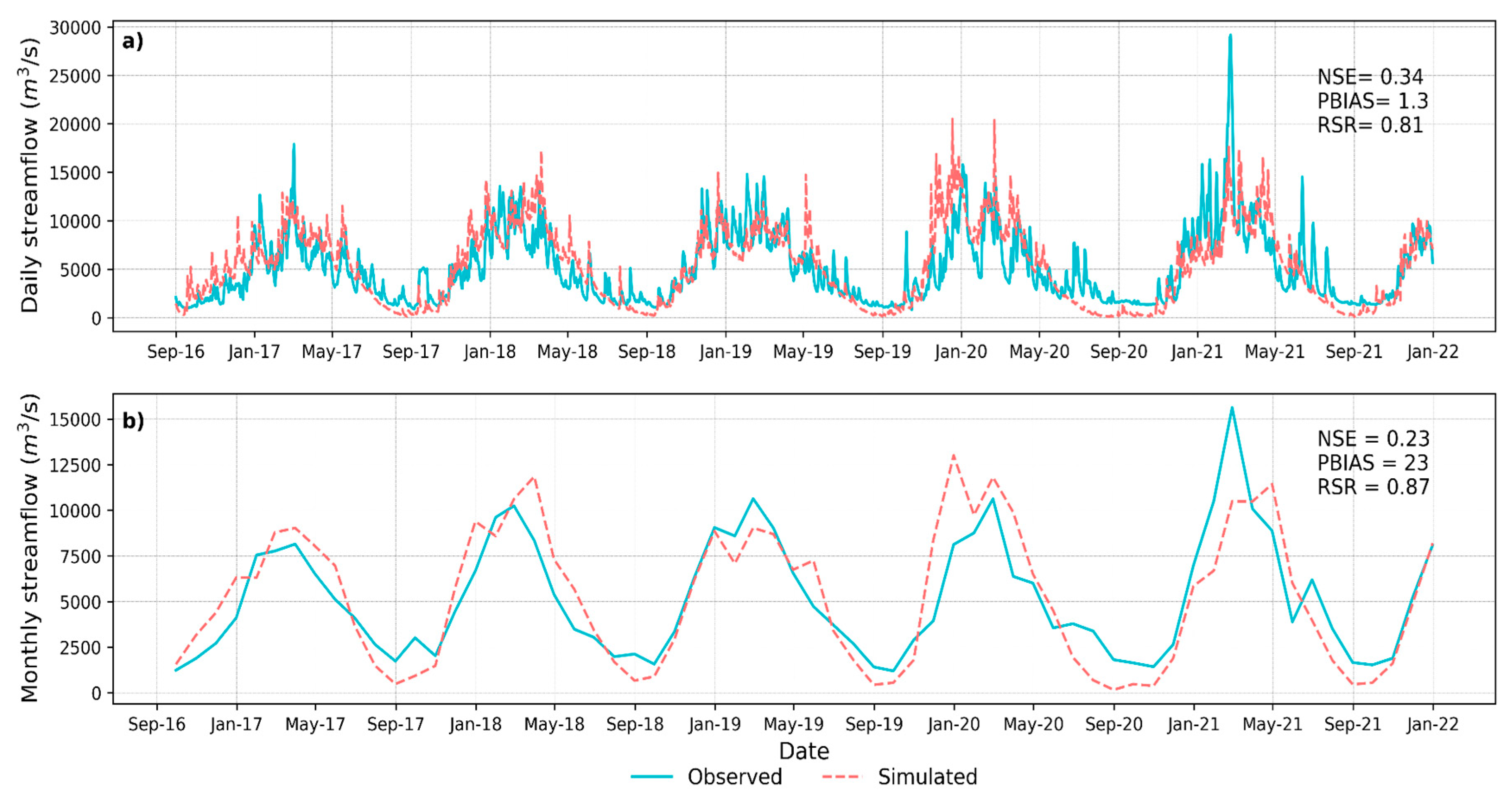
Figure 6 shows the comparison between streamflow data observed and simulated in the first run in a daily and monthly scale.
In order to improve the simulation, an automatic calibration was performed in the SWAT- Calibration Uncertainty Program (CUP) software. The Sequential Uncertainty Fitting (SUFI-2) algorithm was applied with the Nash-Sutcliffe coefficient of efficiency (NS) as the objective function [
46]. One of the first and an important step in automatic calibration is identifying the parameters to optimize [
47]. The parameters chosen are shown in
Table 3 and were selected on the basis of the following analysis.
Figure 3 shows that the simulated streamflow during the dry season is too low against observed flow, this may be related to groundwater water parameters as GWQMN.gw ; GW_REVAP.gw and REVAMPM.gw [
48]. The following two groundwater parameters, GW_DELAY.gw and ALPHA_BF.gw, were chosen because some studies in the Brazilian Amazon report them as sensitive parameters [
15,
16,
49]. ALPHA_BF factor is a constant indicating the response of groundwater flow to any change in recharge (1/day). Values vary from 0.1-0.3 for slow responding lands and 0.9-1.0 for fast responding lands [
14]. Since there are no previous studies on MDD reporting groundwater parameters values, the full ranges for these values were used.
Parameters related to the physical characteristics of the main channel were chosen to be calibrated since these parameters affect the flow of water and transport of sediment in the channel network of the watershed [
14]. The effective hydraulic conductivity (CH_K2.rte) depends on river bed materials, a range of 25-76 mm/hr were used in the calibration corresponding to sand and gravel mixture with low silt-clay content. Manning's "n" coefficient for the main channel (CH_N2.rte) also was calibrated in a meaningful range.
After the sensitivity analysis achieved in SWAT-CUP, 5 parameters were identified as significantly sensitive (p-value < 0.05), including CH_N2.rte, CN2.mgt, GW_DELAY.gw, GWQMN.gw and EPCO.hru. Due to limited data availability regarding these parameters in the MDD basin, ranges of values were established during the calibration process, ensuring they fall within physically meaningful limits. [
14].
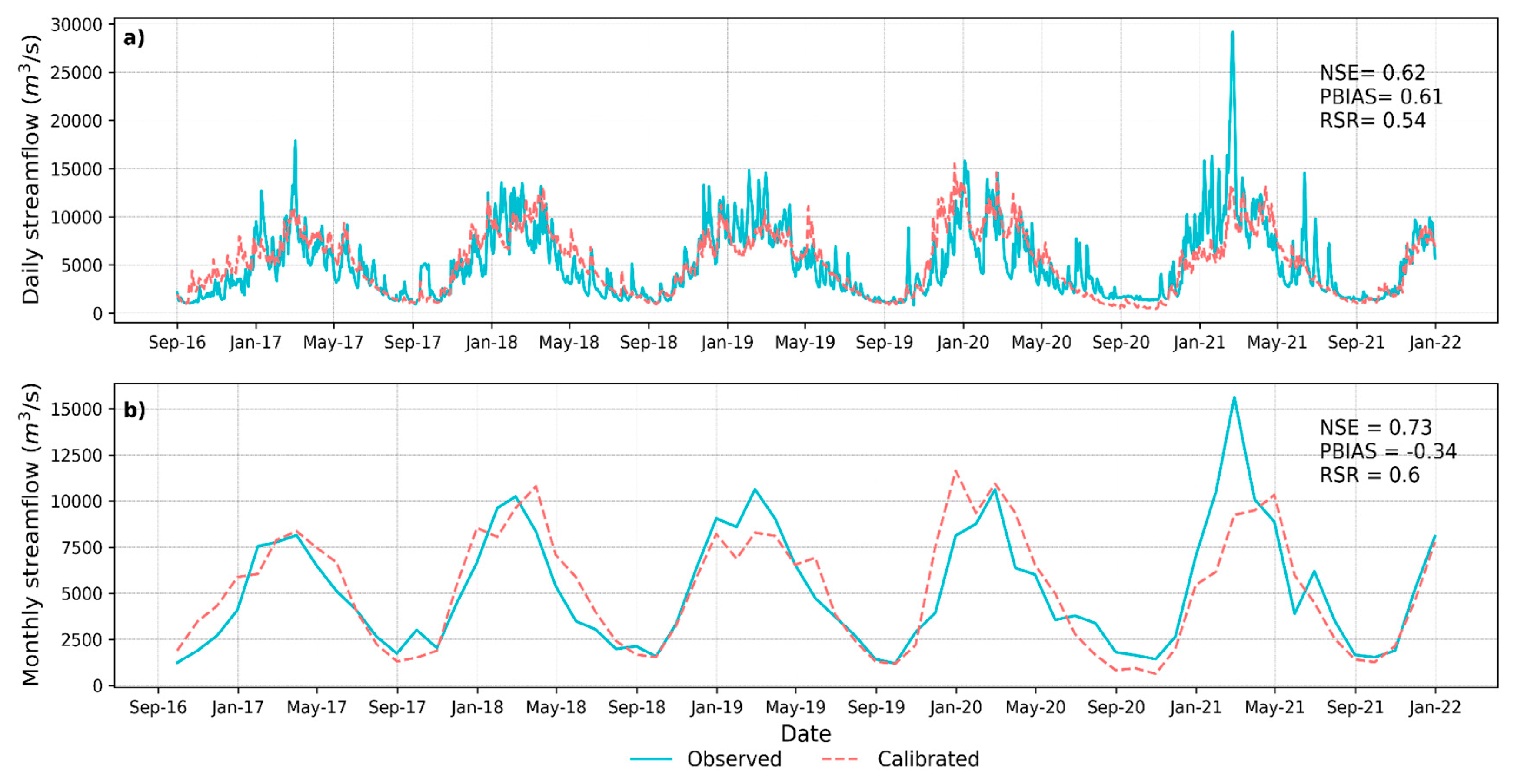
The graphical representation contrasting observed and simulated streamflow during the calibration period (2016-2021) is depicted in
Figure 7. The Nash-Sutcliffe Efficiency (NS) coefficient obtained a value of 0.62 for the daily time step, while for the monthly time step, NS reached 0.73, coupled with a Percent Bias (PBIAS) of 0.5. These values indicate "Good" level of consistency [
41]. Owing to this new calibration step, the model performances improved by 0.28 and 0.8 in terms of NSE and PBIAS, respectively.
3.3. Hydrological basin response corresponding to the Deforestation Scenario simulation.
The simulation was conducted by replacing the original baseline land use map with the deforestation scenario land use map (depicted in
Figure 4) within the calibrated model. This was carried out to analyze the impact of Land Use and Land Cover (LULC) changes on the hydrology of the study area. This modification was implemented while maintaining consistency with the other SWAT inputs, including the Digital Elevation Model (DEM), soil map, and climate data. Within the deforestation scenario, a targeted change was introduced, involving the replacement of 12% of the total area covered by Evergreen Broadleaf Forest (FOEB) with Bare Land (BARR).
3.3.1. Average monthly means
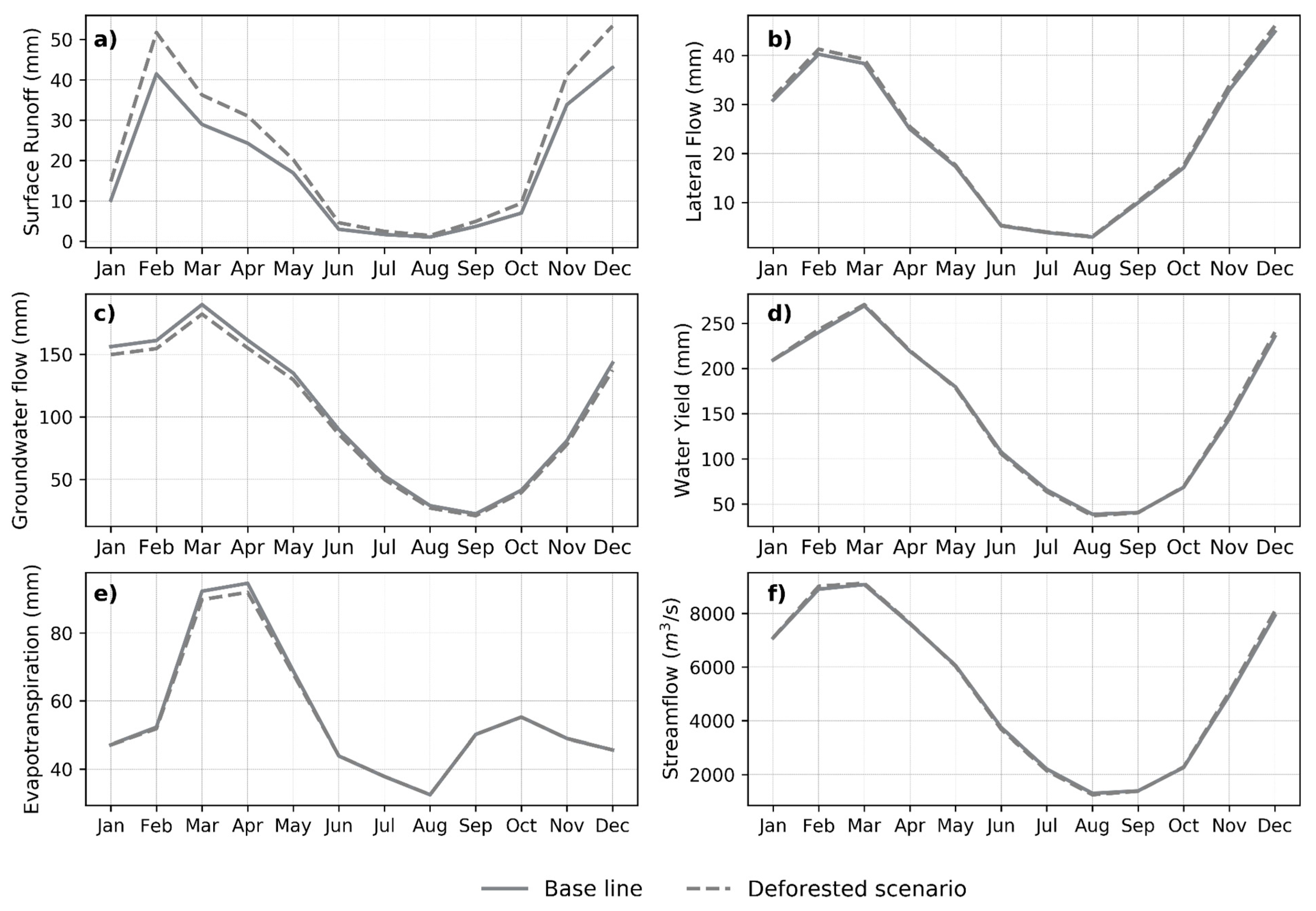
Figure 8 shows the monthly values for the water balance components including surface runoff, lateral flow, groundwater flow, water yield and evapotranspiration in both the baseline and deforestation scenarios. The surface runoff values exhibit their peak from October to April (during the rainy season), while they are at their lowest from May to September (referred to as the dry season).
The monthly impacts of Land Use and Land Cover (LULC) variations from baseline to deforested scenario have been noted on surface runoff. Conversely, the influence of LULC variations on the monthly values of lateral flow, groundwater, water yield, and evapotranspiration is comparatively minor.
Table 4 displays the percentage changes.
Surface runoff indicates a monthly average increase of 33%, with its most significant increases taking place during the dry season (May to September) at a rate of 38%, and the least notable increments occurring during the wet season (October to April) at 29%. Lateral flow has experienced a slight increase of 3%, primarily during the period from July to December. Notably, water yield displays distinct variations between seasons, with a 1% increase during the dry season and a 2% decline during the wet season. An evident decrease in evapotranspiration is observed, especially during the period from February to May, with a reduction of 2%. Likewise, there has been an average monthly decrease of 5% in groundwater flow.
3.2.2. Average annual means
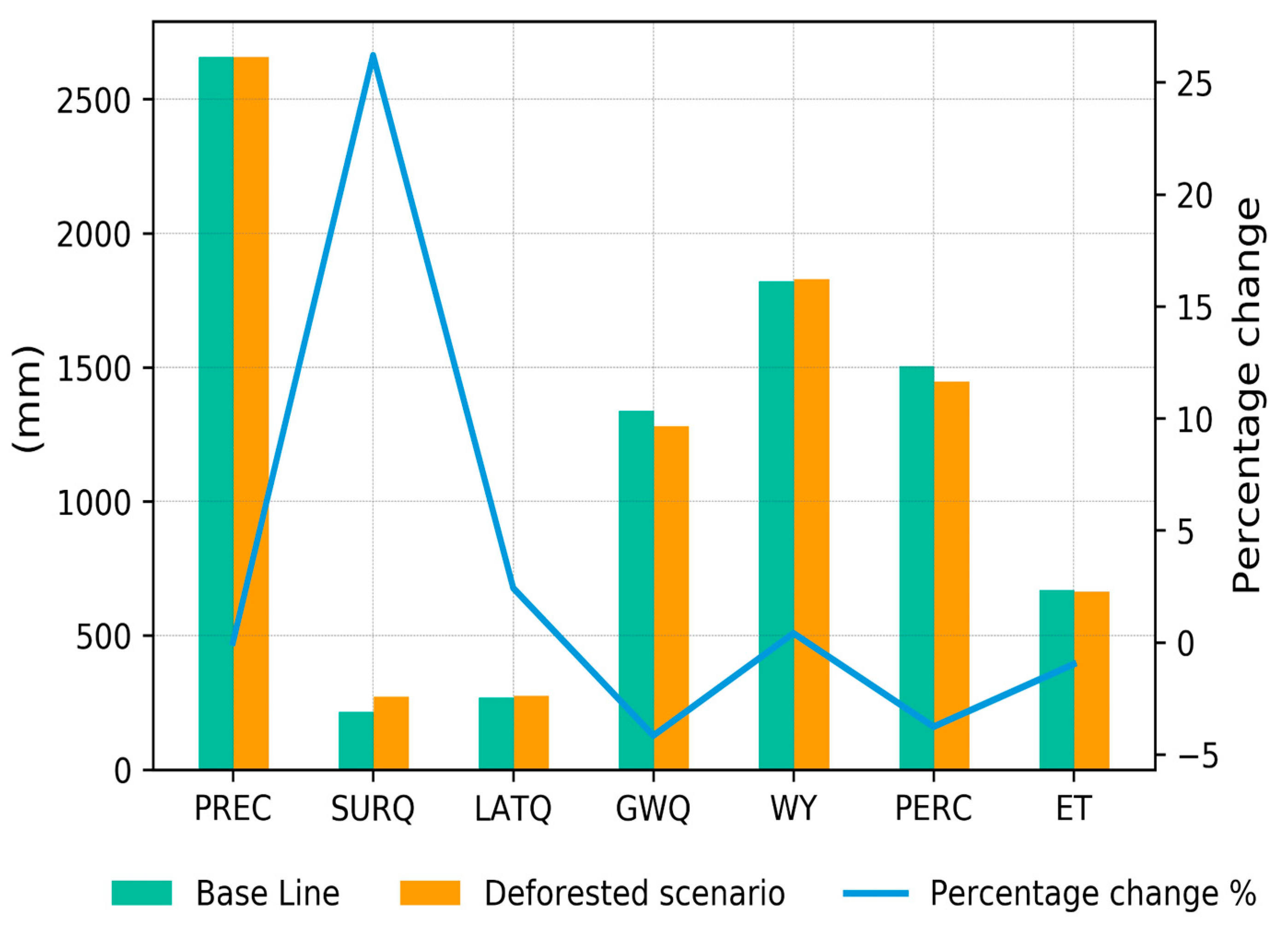
Table 5 depicts the effects of land cover change on the MDD basin. The findings demonstrate that, under both scenarios, there is an increase in the average annual surface runoff, lateral flow, and water yield by 26.2%, 2.4%, and 0.4%, respectively, between both scenarios. Conversely, groundwater flow, percolation, and evapotranspiration decrease by 4.2%, 3.8%, and 1%, respectively. These changes were attributed to the conversion of forest to bare land in the Deforested scenario, as other climate and soil components were kept constant.
Figure 9 provides a summary of the changes in annual water balance components.
3.2.3. Average annual means at subbasin scale.
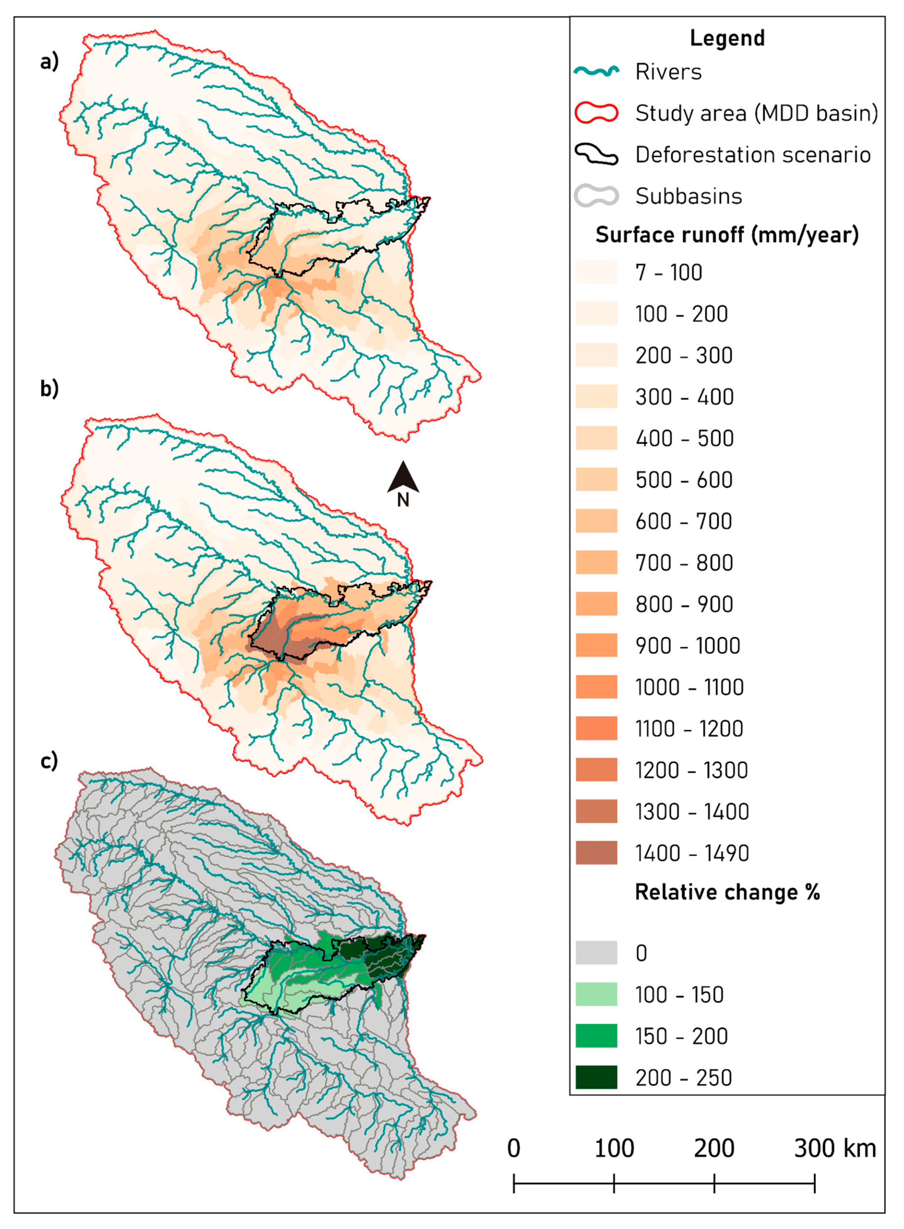
Figure 10 displays the alterations in average annual surface runoff at a subbasin scale. The main changes exhibit consistency within the region where the land cover change was implemented for the deforested scenario. This deforested area had an impact on a total of 26 subbasins, all of which observed an average annual surge of 164% in surface runoff. Among these, the subbasin of the Inambari River demonstrated a notable increase of 187%
.
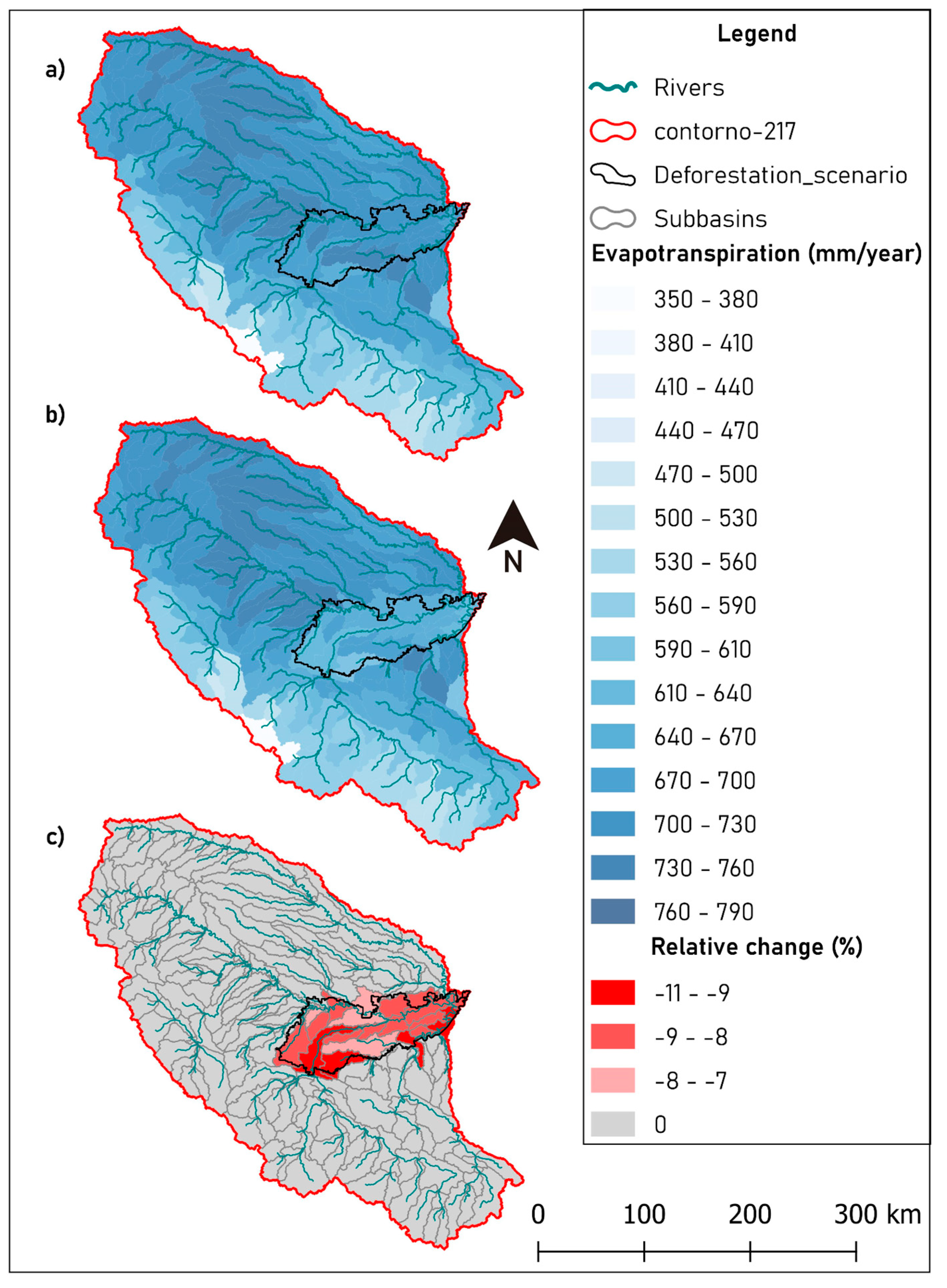
Figure 11 shows the changes in average annual evapotranspiration at the subbasin scale. Just as observed with surface runoff trends, this decline is particularly pronounced within the deforested region. Among the subbasins, one that stands out for its considerable impact is the lower segment of the Inambari River subbasin, where there was a notable 8% reduction in evapotranspiration. Moreover, it is noteworthy that, in average, the subbasins that encountered alterations experienced a decrease of 7% in their annual average evapotranspiration.
4. Discussion
Deforestation within the MDD basin persists as a threat that impacts the environment from multiple perspectives. Unfortunately, the watershed still lacks comprehensive hydrological information. To address this gap, hydrological modeling was executed to investigate how water balance components react to increasing deforestation levels.
The uncertainty within the simulations originates from the initial input data (such as precipitation and temperature information) fed into the model, and this uncertainty becomes particularly evident during the calibration phase. Nevertheless, the refinement of parameters based on the physical attributes of the basin proved instrumental in enhancing model performance, yielding commendable statistical outcomes.
The Land Use and Land Cover (LULC) alteration examined in this study encompassed the Deforestation scenario. This scenario entailed the substitution of 12% of the evergreen broadleaf forest area with bare land, constituting 9% of the total study area. This modification resulted in both temporal and spatial changes in hydrological variables when contrasted with a baseline scenario. The process of deforestation initiates a reduction in interception, thereby contributing to a greater availability of water for infiltration and runoff processes.
The impacts of Land Use and Land Cover (LULC) changes on surface runoff, water yield, groundwater flow, and lateral flow are distinctly noticeable in both annual and monthly average values. However, the effect of LULC on surface runoff is more pronounced in comparison to the other components, whether considering monthly or annual scales.
Surface runoff has a monthly average increase of 33% over the basin; this increment is more noticeable during the dry season (38%) than the wet season (29%). This hydrological component remained the biggest increase in the annual average with 26%. At the subbasin scale, there is a consistent increment in surface runoff within the deforested area, impacting a total of 26 subbasins. This influence is particularly notable on one of the primary tributaries of the Madre de Dios River, the Inambari River, in which basin the average increase reaches a substantial 187% annually. Such change is likely to cause unprecedented floods that are likely to have strong human and economic impacts [
50], especially when cities expand over susceptible to flooding areas [
51].
The increase of surface runoff, consequently increases the monthly streamflow by 12% in the outlet of the basin. Increases in streamflow can lead to flooding and extreme inundation events as has already occurred in the MDD region.
The effects of the loss of forest is also evident in the reduction of the monthly average evapotranspiration by 2% during the period from February to May. When considering the spatial scale it is noticeable that the change is uniformly distributed over the deforested area, the subbasins that encountered alterations experienced a decrease of 7% in their annual average evapotranspiration.
The impact of LULC alteration on soil water content and lateral flow reveals smaller increments, both on a monthly and annual scale. In contrast, groundwater experiences a consistent decline, evident across both monthly observations and yearly trends. These outcomes align with anticipated patterns when forested regions transition to barren soil or alternative forms of land cover, as reported in prior studies [
52]. It is worth emphasizing that subbasins within the deforested area exhibit substantial localized changes, which might not be fully captured in the average values across the broader study area. This demonstrates that forested land possesses the highest capacity for water yield and evaporation, while bare land exhibits the lowest evaporation and the highest surface runoff production capacity. These findings align with conclusions drawn from previous studies [
13,
16,
52,
53,
54].
These results do not take into account other causes of deforestation, such as logging and agriculture. Therefore, more accurate predictions of land cover change in the future would be important to assess the change in hydrology at a deeper level.
5. Conclusions
This study implemented the hydrological model SWAT to assess the impact of deforestation in the hydrology of the MDD basin. The gridded precipitation of the daily CHIRPS product is currently the best option to represent the seasonality of rainfall in the study area. The calibration of the model was conducted respecting the limits of physically meaningful parameters. The parameters related to groundwater were shown to be the most sensitive in the calibration process. A good rating was obtained for the performance of the monthly model (NS = 0.73 and PBIAS= 0.6). The "Deforestation Scenario" was based on the deforestation alerts implemented by the Peruvian Ministry of Environment and was limited to the mining corridor area (9% of the study area).
The deforested scenario alters the hydrology of the MDD basin. The observed alterations exhibit a more pronounced contrast when examined on a monthly basis rather than an annual one. Notably, during the dry season, there is a substantial 38% increase in surface runoff, while in the wet season, there is a marginal 2% reduction in evapotranspiration. Conversely, variables such as lateral flow, groundwater flow, and water yield manifest negligible adjustments, all falling below the 3% threshold, both in annual and monthly assessments. On a spatial scale, the most conspicuous effects are evident in surface runoff and evapotranspiration variables, particularly within the deforestation scenario, impacting a total of 26 sub-basins. Among these, the Inambari river basin stands out as the most severely affected, witnessing a substantial annual increase of 187% in runoff and a concurrent annual decrease of 7% in evapotranspiration.
To enhance the outcomes of this study, it is imperative to augment the hydroclimatological measurement network. This should include a comprehensive assessment of sediment measurements in rivers to facilitate the calibration of these crucial variables, with potential implications for hydrobiological conservation efforts. The documented rise in surface runoff, as established in this research, could potentially impede future reforestation initiatives owing to heightened soil erosion rates. Furthermore, imposing stringent conservation measures is of paramount importance for safeguarding the Amazonian forests. Subsequent investigations should also encompass the analysis of additional factors like sediment concentration and sediment yield, utilizing state-of-the-art remote sensing products for a more comprehensive understanding of the ecosystem dynamics.
References
- Ceballos, G.; & Ehrlich, P. R. Global mammal distributions, biodiversity hotspots, and conservation. Proceedings of the National Academy of Sciences 2006, vol. 103, no 51, p. 19374-19379. [CrossRef]
- Markham, K. E.; Sangermano, Florencia. Evaluating wildlife vulnerability to mercury pollution from artisanal and small-scale gold mining in Madre de Dios, Peru. Tropical Conservation Science 2018, vol. 11, p. 1940082918794320. [CrossRef]
- Myers, N.; Mittermeier, R. A.; Mittermeier, C. G.; Da Fonseca, G. A.; & Kent, J. . Biodiversity hotspots for conservation priorities. Nature 2000, vol. 403 ,no 6772, p. 853-858. [CrossRef]
- Asner, G. P.; Knapp, D. E.; Martin, R. E.; Tupayachi, R.; Anderson, C. B.; Mascaro, J., ... & Silman, M. R. Targeted carbon conservation at national scales with high-resolution monitoring. Proceedings of the National Academy of Sciences 2014, 111(47), E5016-E5022. [CrossRef]
- Asner, G. P.; & Tupayachi, R.. Accelerated losses of protected forests from gold mining in the Peruvian Amazon. Environmental Research Letters 2017, 12(9), 094004. [CrossRef]
- Telmer, K. H.; & Veiga, M. M. World emissions of mercury from artisanal and small scale gold mining. In Mercury fate and transport in the global atmosphere: emissions, measurements and models 2009, (pp. 131-172). Boston, MA: Springer US.
- Ashe, K.. Elevated mercury concentrations in humans of Madre de Dios, Peru. PloS one 2012 , 7(3), e33305. [CrossRef]
- Martinez, G.; McCord, S. A.; Driscoll, C. T.; Todorova, S.; Wu, S.; Araújo, J. F.; ... & Fernandez, L. E. Mercury contamination in riverine sediments and fish associated with artisanal and small-scale gold mining in Madre de Dios, Peru. International journal of environmental research and public health 2018, 15(8), 1584. [CrossRef]
- Gonzalez, D. J.; Arain, A.; & Fernandez, L. E.. Mercury exposure, risk factors, and perceptions among women of childbearing age in an artisanal gold mining region of the Peruvian Amazon. Environmental research 2019, 179, 108786. [CrossRef]
- Gerson J., Topp S.; Vega C.M.; Gardner J.; Yang X.; Fernández L.E; Bernhardt E.; Pavelsky T. Artisanal gold mining ponds amplify mercury risk in the peruvian amazon (Research Brief CINCIA #7) 2021, Puerto Maldonado, Perú: Centro de Innovación Científica Amazónica.
- Caballero, J.; Messinger, M.; Román-Dañobeytia, F.; Ascorra, C.; Fernandez, L. E.; & Silman, M. Deforestation and forest degradation due to gold mining in the Peruvian Amazon: A 34-year perspective. Remote Sensing 2018, vol. 10, no 12, p. 1903. [CrossRef]
- Householder, J. E.; Janovec, J. P.; Tobler, M. W.; Page, S., & Lähteenoja, O. Peatlands of the Madre de Dios River of Peru: distribution, geomorphology, and habitat diversity. Wetlands 2012, 32, 359-368. [CrossRef]
- Liang, J.; Wu, K., Li; Y., Wei, Z.; Zhuo, P.; Yan, Q.; & Luo, X. Impacts of large-scale rare earth mining on surface runoff, groundwater, and evapotranspiration: A case study using SWAT for the Taojiang River Basin in Southern China. Mine Water and the Environment 2019, 38(2), 268-80. [CrossRef]
- Arnold, J.; Kiniry, J.; Srinivasan, R., Williams, J.; Haney, E.; Neitsch, S. 2012a. Soil and Water Assessment Tool: Input/Output Documentation Version 2012. Texas Water Resources Institute.
- De Oliveira Serrão, E. A., Silva, M. T., Ferreira, T. R., de Ataide, L. C. P., dos Santos, C. A., de Lima, A. M. M., ... & Gomes, D. J. C. Impacts of land use and land cover changes on hydrological processes and sediment yield determined using the SWAT model. International Journal of Sediment Research 2022, 37(1), 54-69.
- Abe, C. A.; Lobo, F. D. L.; Dibike, Y. B.; Costa, M. P. D. F;, Dos Santos, V. & Novo, E. M. L. Modeling the effects of historical and future land cover changes on the hydrology of an Amazonian basin. Water 2018, 10(7), 932. [CrossRef]
- Baker, T. J., & Miller, S. N. Using the Soil and Water Assessment Tool (SWAT) to assess land use impact on water resources in an East African watershed. Journal of hydrology 2013, 486, 100-111. [CrossRef]
- Fassoni-Andrade, A. C.; Fleischmann, A. S.; Papa, F.; Paiva, R. C. D. D.; Wongchuig, S.; Melack, J. M.; ... & Pellet, V. Amazon hydrology from space: scientific advances and future challenges. Reviews of Geophysics 2021, 59(4), e2020RG000728. [CrossRef]
- Tuo, Y.; Duan, Z.; Disse, M.; & Chiogna, G. Evaluation of precipitation input for SWAT modeling in Alpine catchment: A case study in the Adige river basin (Italy). Science of the total environment 2016, 573, 66-82. [CrossRef]
- Huffman, G. J.; Bolvin, D. T.; Nelkin, E. J.; Wolff, D. B.; Adler, R. F.; Gu, G., ... & Stocker, E. F. The TRMM multisatellite precipitation analysis (TMPA): Quasi-global, multiyear, combined-sensor precipitation estimates at fine scales. Journal of hydrometeorology 2007, 8(1), 38-55. [CrossRef]
- Schwaller, M. R. and Morris, K. R. A Ground Validation Network for the Global Precipitation Measurement Mission, Journal of Atmospheric and Oceanic Technology. 2011, 28, 301–319. [CrossRef]
- Funk, C.; Verdin, A.; Michaelsen, J.; Peterson, P.; Pedreros, D.; & Husak, G. A global satellite-assisted precipitation climatology. Earth System Science Data 2015, 7(2), 275-287. [CrossRef]
- Paiva, R. C.; D. C. Buarque, W. Collischonn, M.-P. Bonnet, F. Frappart, S. Calmant, and C. A. B. Mendes. Large- scale hydrologic and hydrodynamic modeling of the Amazon River basin, Water Resour. 2013. Res., 49, 1226–1243. [CrossRef]
- Zubieta, R.; Getirana, A.; Espinoza, J. C.; Lavado-Casimiro, W., & Aragon, L. Hydrological modeling of the Peruvian–Ecuadorian Amazon Basin using GPM-IMERG satellite-based precipitation dataset. Hydrology and Earth System Sciences 2017, 21(7), 3543-3555. [CrossRef]
- Balcázar, L.; Bâ, K. M.; Díaz-Delgado, C; Quentin, E.; & Minga-León, S.. Modelado de caudales diarios en una cuenca del sur del Ecuador con precipitación y temperatura estimadas por satélite. Agrociencia 2019, 53(4), 465-486.
- CPC Global Unified Temperature data provided by the NOAA PSL, Boulder, Colorado, USA. Available online: https://psl.noaa.gov (accessed on 29 March 2023).
- Castro, A.; Dávila, C.; Laura, W.; Cubas Saucedo, F.; Ávalos, G.; López, C.; Villena, D.; Valdez, M.; Urbiola, J.; Trebejo, I.; Menis, L.; Marin, D. Climas del Perú: mapa de clasificación climática nacional.Servicio Nacional de Meteorología e Hidrología del Perú (SENAMHI) 2021. Available online: https://pesquisa.bvsalud.org/portal/resource/pt/biblio-1292421 (accessed on 10 December 2021).
- Finer, M.; Ariñez, A.; Mamani, N. Deforestación por Minería de Oro en la Amazonía 2023. MAAP: 178. Available online: https://maaproject.org/2023/mineria-amazonia/ (accessed on 3 March 2023).
- Hansen M.C., Potapov P. V., Moore R., Hancher M., Turubanova S. A., Tyukavina A., Thau D., Stehman S.V., Goetz S.J., Loveland T.R., Kommareddy A., Egorov A., Chini L., Justice C.O., Townshend J.R.G. (2013) High-resolution global maps of 21-st-century forest cover change. Science, 342, 850-853. Available online: https://www.globalforestwatch.org/map/ (accessed on 24 July 2023).
- Infografías de los datos de la cobertura y pérdida de bosques al 2018. Programa Nacional de Conservación de Bosque para la Mitigación del Cambio Climático 2019. Available online: https://sinia.minam.gob.pe/documentos/infografias-datos-cobertura-perdida-bosques-2018. (accessed on 31 January 2023).
- Aybar, C.; Fernández, C.; Huerta, A.; Lavado, W.; Vega, F. & Felipe-Obando, O. Construction of a high-resolution gridded rainfall dataset for Peru from 1981 to the present day. Hydrological Sciences Journal 2020, 65(5), 770-785. [CrossRef]
- Observatorio del Agua. Sistema Nacional de Información de los Recursos Hídricos. Autoridad Nacional del Agua. Available online: https://snirh.ana.gob.pe/ObservatorioSNIRH/ (accessed on 12 August 2022).
- Farr, T. G.,et al. The shuttle radar topography mission, Rev. Geo-phys. 2007, 45, RG2004. [CrossRef]
- FAO. Soil Map of the World. United Nations Educational, Scientific, and Cultural Organization, Paris, UNESCO 1995.
- USGS. Global Land Cover Characterization; United State Geological Survey: Washington, DC, USA, 1997. [Google Scholar]
- Arnold, J. G.; Srinivasan, R.; Muttiah, R. S.; & Williams, J. R. Large area hydrologic modeling and assessment part I: model development 1. JAWRA Journal of the American Water Resources Association 1998, 34(1), 73-89. [CrossRef]
- Gassman, P. W.; Reyes, M. R.; Green, C. H.; & Arnold, J. G. The soil and water assessment tool: historical development, applications, and future research directions. Transactions of the ASABE 2007, 50(4), 1211-1250. [CrossRef]
- Neitsch, S. L.; Arnold, J. G.; Kiniry, J. R.; & Williams, J. R. Soil and water assessment tool theoretical documentation version 2009. Texas Water Resources Institute 2011. Available online: https://swat.tamu.edu/media/99192/swat2009-theory.pdf (accessed on 10 June 2021).
- Dile, Y. T.; Daggupati, P.; George, C.; Srinivasan, R.; & Arnold, J. Introducing a new open source GIS user interface for the SWAT model. Environmental modelling & software 2016, 85, 129-138. [CrossRef]
- Daggupati, P., Pai, N., Ale, S., Doulgas-Mankin, K.R., Zeckoski, R., Jeong, J., Parajuli, P., Saraswat, D., Youssef, M. A recommended calibration and validation strategies for hydrological and water quality models. Transactions of the ASABE 2015, 58 (6), 1705e1719.
- Moriasi, D. N.; Arnold, J. G.; Van Liew, M. W.; Bingner, R. L.; Harmel, R. D.; & Veith, T. L. Model evaluation guidelines for systematic quantification of accuracy in watershed simulations. Transactions of the ASABE 2007, 50(3), 885-900.
- Nash, J.E.; Sutcliffe, J.V. River flow forecasting through conceptual models: part 1. d A discussion of principles. Journal of Hydrology 1970, 10, 282e290.
- Gupta, H.; Sorooshian, S.; Yapo, P.. Status of automatic calibration for hydro- logic models: comparison with multilevel expert calibration. Journal of Hydrology 1999, Eng. 4, 135e143.
- Moriasi, D. N.; Pai, N.; Steiner, J. L.; Gowda, P. H.; Winchell, M.; Rathjens, H.; Starks, P.J. & Verser, J. A. SWAT-LUT: A desktop graphical user interface for updating land use in SWAT. JAWRA Journal of the American Water Resources Association 2019, 55(5), 1102-1115. [CrossRef]
- Vargas, C.; Montalban, J.; & Leon, A. A. Early warning tropical forest loss alerts in Peru using Landsat. Environmental Research Communications 2019, 1(12), 121002. [CrossRef]
- Abbaspour, K.C. SWAT-CUP: SWAT calibration and uncertainty programs - a user manual. Dübendorf, Switzerland: Eawag, 2015. 103p.
- Abbaspour, K. C.; Vaghefi, S. A.; & Srinivasan, R. A guideline for successful calibration and uncertainty analysis for soil and water assessment: a review of papers from the 2016 international SWAT conference. Water 2017, 10(1), 6. [CrossRef]
- Abbaspour, K. C.; Rouholahnejad, E.; Vaghefi, S. A.; Srinivasan, R.; Yang, H., & Kløve, B. A continental-scale hydrology and water quality model for Europe: Calibration and uncertainty of a high-resolution large-scale SWAT model. Journal of hydrology 2015, 524, 733-752. [CrossRef]
- Strauch, M. & Volk, M. SWAT plant growth modification for improved modeling of perennial vegetation in the tropics. Ecological Modelling 2013, 269, 98-112. [CrossRef]
- Kreibich, H.; Van Loon, A. F.; Schröter, K.; Ward, P. J.; Mazzoleni, M.; Sairam, N.; ... & Di Baldassarre, G. The challenge of unprecedented floods and droughts in risk management. Nature 2022, 608(7921), 80-86. [CrossRef]
- García-Rivero, A. E.; Olivera, J.; Salinas, E.; Yuli, R. A.; & Bulege, W. Use of hydrogeomorphic indexes in SAGA-GIS for the characterization of flooded areas in Madre de Dios, Peru. Int. J. Appl. Eng. Res 2017, 12, 9078-9086.
- Abuhay, W.; Gashaw, T.; & Tsegaye, L. Assessing impacts of land use/land cover changes on the hydrology of Upper Gilgel Abbay watershed using the SWAT model. Journal of Agriculture and Food Research 2023, 12, 100535. [CrossRef]
- Zhang, H.; Wang, B.; Li Liu, D.; Zhang, M.; Leslie, L. M.; & Yu, Q. Using an improved SWAT model to simulate hydrological responses to land use change: A case study of a catchment in tropical Australia. Journal of Hydrology 2020, 585, 124822. [CrossRef]
- Gashaw, T.; Tulu, T.; Argaw, M.; & Worqlul, A. W. Modeling the hydrological impacts of land use/land cover changes in the Andassa watershed, Blue Nile Basin, Ethiopia. Science of the Total Environment 2018, 619, 1394-1408. [CrossRef]
Figure 1.
Study area and location map of the meteorological and hydrological stations.
Figure 1.
Study area and location map of the meteorological and hydrological stations.
Figure 2.
Accumulated monthly precipitation data, mean temperature plotted in the secondary axis and observed monthly streamflow at the hydrological station Amaru Mayu (outlet point of the MDD basin).
Figure 2.
Accumulated monthly precipitation data, mean temperature plotted in the secondary axis and observed monthly streamflow at the hydrological station Amaru Mayu (outlet point of the MDD basin).
Figure 3.
a)Soil type map. Source: Food and Agriculture Organization of the United Nations (FAO). b) Land use cover map. Source: Global Land Cover Characterization (GLCC)- USGS.
Figure 3.
a)Soil type map. Source: Food and Agriculture Organization of the United Nations (FAO). b) Land use cover map. Source: Global Land Cover Characterization (GLCC)- USGS.
Figure 4.
Land use map of the deforestation scenario.Source. Land use map: Global Land Cover Characterization (GLCC)- USGS. Deforestation national alerts :
http://geobosques.minam.gob.pe [
45].
Figure 4.
Land use map of the deforestation scenario.Source. Land use map: Global Land Cover Characterization (GLCC)- USGS. Deforestation national alerts :
http://geobosques.minam.gob.pe [
45].
Figure 5.
Correlation between stream flows generated by SWAT model using CHIRPS, TRMM and PISCO precipitation datasets and in-situ data (Amaru Mayu station).
Figure 5.
Correlation between stream flows generated by SWAT model using CHIRPS, TRMM and PISCO precipitation datasets and in-situ data (Amaru Mayu station).
Figure 6.
a) Daily and b) Monthly time series of observed and simulated streamflow in the first model run forced using CHIRPS rainfall.
Figure 6.
a) Daily and b) Monthly time series of observed and simulated streamflow in the first model run forced using CHIRPS rainfall.
Figure 7.
a) Daily and b) monthly time series of observed and calibrated streamflow in the hydrological station Amaru Mayu, after the calibration process.
Figure 7.
a) Daily and b) monthly time series of observed and calibrated streamflow in the hydrological station Amaru Mayu, after the calibration process.
Figure 8.
Monthly average simulated a) surface runoff (mm) b) lateral flow (mm) c) groundwater flow (mm) d) water yield (mm) e) evapotranspiration (mm) and f) streamflow (m3. s-1).
Figure 8.
Monthly average simulated a) surface runoff (mm) b) lateral flow (mm) c) groundwater flow (mm) d) water yield (mm) e) evapotranspiration (mm) and f) streamflow (m3. s-1).
Figure 9.
Annual average amounts and percentage change in the water balance components in both baseline and deforested scenarios.
Figure 9.
Annual average amounts and percentage change in the water balance components in both baseline and deforested scenarios.
Figure 10.
Annual average surface runoff at sub basin scale in a) baseline and b) deforested scenario. c) Relative percentage change between both scenarios.
Figure 10.
Annual average surface runoff at sub basin scale in a) baseline and b) deforested scenario. c) Relative percentage change between both scenarios.
Figure 11.
Annual average evapotranspiration at sub basin scale in a) baseline and b) deforested scenario. c) Relative percentage change between both scenarios.
Figure 11.
Annual average evapotranspiration at sub basin scale in a) baseline and b) deforested scenario. c) Relative percentage change between both scenarios.
Table 1.
Model input data.
Table 1.
Model input data.
| Input data |
Spatial resolution |
Source |
| Precipitation |
0.05॰(~5 km) |
CHIRPS v2.0 [22] |
| Temperature |
0.5॰ (~55 km) |
CPC Global Unified Temperature[23] |
| Digital Elevation Model |
30 m |
SRTM [33] |
| Soil type map |
1:5000,000 |
FAO v3.6 [34] |
| Land use cover map |
~0.5 km |
GLCC - USGS v2 [35] |
| Observed streamflow |
- |
ANA [32] |
Table 2.
Statistics evaluated for the assessment of streamflow performance in a monthly time step.[
41].
Table 2.
Statistics evaluated for the assessment of streamflow performance in a monthly time step.[
41].
| Performance rating |
NS |
PBIAS |
RSR |
| Very good |
0.75≤ NS ≤1.00 |
PBIAS≤ ± 15% |
0≤ RSR ≤0.5 |
| Good |
0.65≤ NS ≤0.75 |
±15%≤ PBIAS ≤ ± 30% |
0.5≤ RSR ≤0.6 |
| Satisfactory |
0.5≤ NS ≤0.65 |
± 30%≤ PBIAS ≤ ± 55% |
0.6≤ RSR ≤0.7 |
| Unsatisfactory |
NS ≤ 0.5 |
PBIAS ≥ ± 55% |
RSR ≥0.7 |
Table 3.
Parameters included in the sensitivity analysis.
Table 3.
Parameters included in the sensitivity analysis.
| Description |
Parameter |
Default value |
Calibrated range |
Fitted value |
| Curve number for moisture condition II |
CN2.mgt_FOEB1
|
72 |
0-98 |
46.2 |
| CN2.mgt_GRAS1
|
81 |
0-98 |
52.1 |
| CN2.mgt_SHRB1
|
76 |
0-98 |
48.8 |
| Baseflow alpha factor (1/days) |
ALPHA_BF.gw |
0.048 |
0-1 |
1 |
| Threshold depth of water in the shallow aquifer required for return flow to occur (mm H2O). |
GWQMN.gw |
1000 |
0-5000 |
2009.1 |
| Groundwater "revap" coefficient. |
GWREVAP.gw |
0.02 |
0.02-0.2 |
0.08 |
| Threshold depth of water in the shallow aquifer for “revap” or percolation to the deep aquifer to occur (mm H2O). |
REVAPMN.gw
|
750 |
0-500 |
322 |
| Groundwater delay time (days). |
GW_DELAY.gw |
31 |
30-450 |
60.26 |
| Effective hydraulic conductivity in main channel alluvium (mm/hr) |
CH_K2.rte |
0 |
0-250 |
51.4 |
| Manning's "n" value for the main channel. |
CH_N2.rte |
0.014 |
0.01-0.3 |
0.06 |
| Soil evaporation compensation factor. |
ESCO.hru |
1 |
0.01-1 |
0.98 |
| Plant uptake compensation factor. |
EPCO.hru |
0.95 |
0.01-1 |
1 |
| Saturated hydraulic conductivity (mm/hr) |
SOL_K.sol_FOEB1
|
8.93 |
0-2000 |
9.4 |
| SOL_K.sol_GRAS1
|
24.83 |
0-2000 |
26.14 |
| SOL_K.sol_SHRB1
|
37.59 |
0-2000 |
39.6 |
Table 4.
Percent change of monthly average water balance components, including surface runoff (SURQ), lateral flow (LATQ), water yield (WY), evapotranspiration (ET), and groundwater flow (GWQ), under both baseline and deforested scenarios.
Table 4.
Percent change of monthly average water balance components, including surface runoff (SURQ), lateral flow (LATQ), water yield (WY), evapotranspiration (ET), and groundwater flow (GWQ), under both baseline and deforested scenarios.
Hydrological
component |
Jan |
Feb |
Mar |
Apr |
May |
Jun |
Jul |
Aug |
Sep |
Oct |
Nov |
Dec |
| Percent change % |
|---|
| SURQ |
45.7 |
24.7 |
25.2 |
27.8 |
19.4 |
54.5 |
47 |
35.2 |
34.4 |
35.1 |
21.6 |
23.9 |
| LATQ |
2.1 |
2.6 |
2.3 |
2.0 |
1.7 |
1.7 |
2.6 |
3.4 |
3.0 |
2.8 |
2.9 |
2.6 |
| WY |
0.1 |
1.3 |
0.5 |
0.3 |
-0.6 |
-1.9 |
-3.0 |
-4.2 |
-0.8 |
0.8 |
2.5 |
2.1 |
| ET |
-0.04 |
-0.9 |
-2.7 |
-2.8 |
-1.3 |
0.1 |
0.1 |
0.1 |
0 |
-0.1 |
-0.04 |
-0.04 |
| GWQ |
-4.1 |
-4.0 |
-4.0 |
-3.9 |
-3.9 |
-4.3 |
-5.3 |
-6.6 |
-6.6 |
-4.3 |
-3.8 |
-4.0 |
Table 5.
Percent change of the annual average values of the water balance components, including surface runoff (SURQ), lateral flow (LATQ), water yield (WY), evapotranspiration (ET), and groundwater (GWQ), under both baseline and deforested scenarios.
Table 5.
Percent change of the annual average values of the water balance components, including surface runoff (SURQ), lateral flow (LATQ), water yield (WY), evapotranspiration (ET), and groundwater (GWQ), under both baseline and deforested scenarios.
| Scenario |
SURQ |
LATQ |
GWQ |
WY |
PERC |
ET |
| Base Line |
215.6 |
269.1 |
1337.1 |
1821.5 |
1503.8 |
669.8 |
| Deforested scenario |
272.1 |
275.6 |
1281.5 |
1829 |
1447.2 |
663.3 |
| % change |
26.2 |
2.4 |
-4.2 |
0.4 |
-3.8 |
-1 |
|
Disclaimer/Publisher’s Note: The statements, opinions and data contained in all publications are solely those of the individual author(s) and contributor(s) and not of MDPI and/or the editor(s). MDPI and/or the editor(s) disclaim responsibility for any injury to people or property resulting from any ideas, methods, instructions or products referred to in the content. |
© 2023 by the authors. Licensee MDPI, Basel, Switzerland. This article is an open access article distributed under the terms and conditions of the Creative Commons Attribution (CC BY) license (http://creativecommons.org/licenses/by/4.0/).
