Preprint
Article

Implementation of Elzaki HPM for Semi-Analytical Solution upon Two-Dimensional Fuzzy Fractional Heat Equation

Altmetrics

Downloads

116

Views

44

Comments

0

Submitted:

12 September 2023

Posted:

14 September 2023

You are already at the latest version

Alerts
Abstract
In this research, a computation algorithm is established for a fractional order 2D fuzzy heat equation. In this study, Elzaki transform and HPM fusion is produced. Computing the desired outcome in series yields a fast convergence on an appropriate response. Examples are provided to support the conclusions, which are then compared with a particular approach to show the effectiveness and potential of the suggested approach. Two crisp equations—one for the lower bound solution and one for the upper bound solution are constructed from the input fuzzy fractional heat equation. The contour and surface representations of the approximate and exact results are offered for the lower and upper-bound solutions. The l∞-error norm is used in this study to validate the numerical convergence aspect. Together with the absolute inaccuracy, the approximate and exact solutions are matched. It has been demonstrated that the proposed regime will make it feasible to work with fuzzy fractional partial differential equations in a wide range of dimensions.
Keywords: 
Subject: Physical Sciences  -   Mathematical Physics

1. Introduction

In the course of the last few decades, academics and scientists have demonstrated a great deal of interest in the field of fractional calculus (FC), which is concerned with derivatives and integrals of non-integer order. As we know, classical calculus has been developed as a vast subject, and many researchers have been working on it till now. Due to the ideas of German mathematiciansLebiez and L-Hospital, the theory of fractional calculus came into existence about 300 years ago. FC can be assumed to be a well-developed and established subject. Both memory effects and hereditary properties influence the problem under consideration. We all know that classical differential equations have numerous applications that model many natural phenomena and physical phenomena compared to classical differential equations. In the last few decades, an abundance of research papers, monographs, and books have been published, covering an extensive range of subjects such as existence theory and analytical results.For instance, mathematical models involving fractional as well as integer order derivatives have been investigated for different real-world problems in literature (we refer the readers to References [12,13,14,15,16,17,18,19] and the references therein). There are numerous local and nonlocal fractional notions in the literature, notably those of Riemann-Liouville, Grunwald, Caputo, Riesz, conformable and Caputo-Fabrizio. Since most physical implementations rely on historical and nonlocal properties, nonlocal derivatives are more intriguing than local derivatives. On the basis of singular kernels, some of these operations, notably Riemann-Liouville and Caputo have been offered. In contrast to traditional fractional derivatives, recent fractional derivatives that are based on nonsingular kernels that were suggested by Caputo-Fabrizio [6] and Atangana-Baleanu [7] are more accurately represent physical dissipative procedures and minimize a numerical collision. Here, we seek to expand such a tool to examine certain problems which appear in the biological, social, and physical sciences, as well as other areas where there is data inconsistency.
In 1960, Zadeh [8] introduced the concept of the theory of fuzzy sets as an extension of classical set theory. Since then, it has started gaining the attraction of many researchers due to its skillin analyzing unpredictabilityinfacts and particulars. Mainly, fuzzy set theory allows us to prospect new estimations and expand the chances for effectively handling and analyzing fuzzy information. Fuzzy mapping and control were developed by Chang and Zadeh [9] and the concept of the fuzzy set was further developed upon. A number of researchers generalized this notion in order to build primary fuzzy calculus on the basis of fuzzy mapping and control [10,11,12]. Fuzzy calculus deals with fuzzy sets and fuzzy numbers, allowing for representing and manipulating unpredictable and unspecific quantities. Fuzzy calculus is being found applicable in a wide range of fields, including mathematics, computer science and engineering. Numerous fields, including topology, fixed-point theory, integral inequalities, fractional calculus, bifurcation, image processing, pattern recognition, expert systems, consumer electronics, control theory, artificial intelligence, and operations research have made extensive use of the fuzzy calculus. Fuzzy fractional differential and integral equations (FFDIEs) have received significant attention in the physical sciences during the past few decades. Among those who initially proposed the fundamental idea of fuzzy integral equations were Dobius and Prada [13]. To deal with such types of challenges, as the information is unclear and unreliable, fuzzy numbers are employed for parameters instead of crisp numbers. FFDIEs may be employed to model these types of concerns. As a consequence, many researchers evaluated such model’s details through numerical or analytical techniques.
Nowadays, academics and scientists have demonstrated a great deal of interest in the field of fuzzy fractional calculus (FFC), which is an augmentation of fractional calculus and fuzzy calculus. It broadens the conventional calculus operations, such as differentiation and integration, to fuzzy numbers of arbitraryorder. This allows for a more comprehensive analysis of functions and systems that exhibit both fuzzy and fractional characteristics. Research in FFC continues to explore new theoretical developments, such as the establishment of fuzzy fractional differential equations and the development of appropriate techniques for solving them. This provides a more accurate and powerful tool for modeling and analyzing complex systems with fractional and fuzzy characteristics, allowing for a better mastery and control of real-world phenomena. Fuzzy fractional calculus has been applied in areas such as finance, image processing, control systems, and others.For example, fuzzy fractional operators can be used to upgrade image characteristics and grasp noise or unpredictability of the data in image processing. Fuzzy fractional derivatives heavily rely on fuzzy Riemann–Liouville or fuzzy Caputo-Liouville derivative.Many fuzzy fractional differential operators are known to be nonlocal, indicating that their future states depend on their historical and current situations. A range of singular and non-singular fuzzy fractional operators have been developed with applications in a wide range of fields of science [5,6,7,8,9,10]. The nonlocality and singularity of the kernel function, which can be seen in the integral operator’s side-by-side with the normalizing function arising alongside the integral ticks, are the most prevalent shortcomings of these two qualifiers. Indeed, a more useful and clear definition must result from the unpreventable existence of real-world core reproducing dynamic fractional systems. Atangana-Baleanu-Caputo (ABC), a novel fractional fuzzy derivative construct that is utilized to synthesize and convey fresh tangible fuzzy mathematical concepts, is introduced in this orientation. The new fuzzy fractional ABC derivative appears to be releasing singularity with the local kernel function. This is because the kernel is based on the nature of exponential decay, making fuzzy fractional order differential equations (FFPDEs) more plausible in establishing several uncertain models [1,2,3,4,5].
Further, FFPDEs have many real-world problems like heat transfer phenomena, nonlinear propagation of traveling waves, damped nonlinear string, electronics, telecommunications, dynamical systems and so on(see References [36–38]).To tackle FFPDEs, important tools and methods were found in the literature. Such tools include Fourier integral transform, Laplace transform, Sumudu transform, and so on. Among others, we found some analytical methods like Homotopy methods, Adomian decomposition, Laplace Adomian decomposition methods, Taylor’s series method, and other methods.In [31], the homotopy analysis transform method has been proposed and implemented to derive new analytical solutions for the fuzzy heat-like equations. To the best of our information, the above mentioned methods have not been properly used to deal with FFPDEs.
On the other hand, perturbation methods are important tools for solving nonlinear problems. However, these methods, like other nonlinear analytical techniques, have their own set of restrictions. That is, the applicability of perturbation techniques is severely limited by the assumption that the Equation must have a small parameter. The Homotopy Perturbation Method (HPM),which is the coupling of the homotopy method and classical perturbation technique, was first proposed by He [21] and then used by many researchers in recent years to solve various types of linear and nonlinear differential equations, see, for example, [22,23] and references therein. The main significance of this method is that it doesn’t require a small parameter in the Equation, so it overcomes the impediments of the classical perturbation technique. In 2020, Muhammad Arfan et al. developed an algorithm based on the HPM to compute an analytical solution for a two-dimensional fuzzy fractional heat equation involving external source term, and found the efficiency and the capability of the method. The Laplace transform, decomposition techniques, and the Adomian polynomial under the Caputo–Fabrizio fractional differential operator have been applied to obtain the semi-analytical solution of the 2D heat equation without an external diffusion term.
In [20], the authors applied the HPM along with a crucial integral transform called Elzaki transformation (ET) to provide the solution of some nonlinear partial differential equations. This method is called the Homotopy Perturbation Elzaki Transform method (HPETM). This method gives a power series solution in the form of a rapidly convergent series lead to high accurate solutions with only a few iterations. The efficiency of HPETM in solving nonlinear homogeneous and non-homogeneous partial differential equations is also shown in [24,25,26].
In the present work, we focus on computingan approximate solution by the iterativemethod based HPETM for the following two-dimensional fuzzy fractional heat equation:
D t α u ~ μ , ν , t = u ~ x x μ , ν , t + u ~ y y μ , ν , t + f μ , ν , t ,   0 < α 1 ,
u ~ μ , ν , 0 =   g ~ μ , ν ,
where α stands for Caputo fractional derivativeand f C 0 ,   × 0 ,   × 0 ,   ,   0 ,   ,   g ~ 0 ,   × 0 ,   , 0 ,   . It is pointed out that, the two-dimensional heat equation representsthe transfer of heat through an infinite thin sheet. Here in Equation (1), the term u ~ represents the temperature of the body at any point in the thin sheet. This phenomenon of heat transfer can be found in many diffusion problems. Therefore, the investigation of two-dimensional Fuzzy fractional heat equationshas much more application in various domains, such as heat transfer analysis in materials with uncertain properties, modeling of temperature distribution in environmental systems, or analysis of thermal processes in complex systems with imprecise parameters.
The two crisp fuzzy fractional equations will be fetched as follows:
D t α u _ μ , ν , t = u _ x x μ , ν , t + u _ y y μ , ν , t + f μ , ν , t ,
u _ μ , ν , 0 =   g _ μ , ν ,
and
D t α u ¯ μ , ν , t = u ¯ x x μ , ν , t + u ¯ y y μ , ν , t + f μ , ν , t ,
u ¯ μ , ν , 0 =   g ¯ μ , ν .
For HPM, the considered Equation is as follows:
D u = 0 ,
where D is considered as a differential operator, any convex Homotopy deformation H ( u ,   p ) is as follows:
H u ,   p = 1 p F u + p   D u ,
where F ( u ) is considered as a basic operator with the known solution u 0 .
In such an approach, embedding parameter ‘ p ’ is used initially, and the solution of the Equation is provided in the form of a power series.
U = u 0 + p   u 1 + p 2 u 2 + p 3 u 3 + + p n u n ,
U = lim p 1 U ,
U = u 0 + u 1 + u 2 + u 3 + + u n ,
U = lim p 1 U ,
U = n = 0 u n ,
This helps us to obtain the solution.

2. Preliminaries

In this section, the most basic notations used in this paper are introduced.
Definition 1.
For all fuzzy numbers, the lower and upper bounds of the fuzzy numbers satisfy the following requirements [27]:
(i)
u _ ( r ) is a bounded left-continuous nondecreasing function over [0, 1],
(ii)
u ¯ ( r ) is a bounded right-continuous nonincreasing function over [0, 1],
(iii)
u _ ( r )     u ¯ ( r )   , 0     r     1
Definition 2.
Fuzzy center of an arbitrary fuzzy number u ~ = [ u _ ( r ) , u ¯ ( r ) ] is defined as [27]:Preprints 84942 i001
Definition 3.
Fuzzy radius of an arbitrary fuzzy number u ~ = [ u _ ( r ) , u ¯ ( r ) ] is defined as [27]:Preprints 84942 i002
Definition 4.
Fuzzy width of an arbitrary fuzzy number u ~ = [ u _ ( r ) , u ¯ ( r ) ] is defined as [27]:Preprints 84942 i003
Definition 5.
For any two arbitrary fuzzy numbers x ~ = [ x _ ( r ) , x ¯ ( r ) ] , y ~ = [ y _ ( r ) , y ¯ ( r ) ] andscalar k , the fuzzy arithmetic is similar to the interval arithmetic defined as follows:
(i)
x ~ = y ~ if and only if x _ ( r ) = y _ ( r ) and x ¯ r = y ¯ r ,
(ii)
x ~ + y ~ = x _ r + y _ r , x ¯ r + y ¯ r .
Definition 6.
Let ϕ : R E is a fuzzy valued function s.t. r 0,1 [28]
ϕ ξ r = ϕ r ξ _ ,     ϕ r ξ ¯ :
  • If ϕ(ξ) is a differentiable function in the first form i.e., (1) differentiable, then
Preprints 84942 i004
2.
If ϕ(x) is a differentiable function in second form i.e., (2) differentiable, then
Preprints 84942 i005
Definition 7.
Let ϕ : a , b E is said to be a strongly generalized H differentiable function at ξ 0 a , b if there exists ϕ ξ 0 E such that for h > 0 and close to zero [28]
  • ϕ ξ 0 = lim h 0 ϕ ξ 0 + h Θ ϕ ξ 0 h = lim h 0 ϕ ξ 0 Θ ϕ ξ 0 h h ,
  • ϕ ξ 0 = lim h 0 ϕ ξ 0 Θ ϕ ξ 0 + h h = lim h 0 ϕ ξ 0 h Θ ϕ ξ 0 h ,
  • ϕ ξ 0 = lim h 0 ϕ ξ 0 + h Θ ϕ ξ 0 h = lim h 0 ϕ ξ 0 h Θ ϕ ξ 0 h ,
  • ϕ ξ 0 = lim h 0 ϕ ξ 0 Θ ϕ ξ 0 + h h =   lim h 0 ϕ ξ 0 Θ ϕ ξ 0 h h .
Definition 8.
Let ϕ ξ , ϕ ξ , , ϕ n 1 ( ξ )   are differentiable fuzzy valued functions with r-cut form [28]
ϕ ξ r = ϕ r ξ _ ,     ϕ r ξ ¯ .
  • If ϕ ξ , ϕ ξ , , ϕ n 1 ( ξ )   are (1) differentiable, then
    ϕ n ξ r = ϕ r n ξ _ ,     ϕ r n ξ ¯ .             )
  • If ϕ ξ , ϕ ξ , , ϕ n 1 ( ξ )   are (2) differentiable, then
    ϕ n ξ r = ϕ r n ξ _ ,     ϕ r n ξ ¯ .
  • If ϕ ( ξ ) is (1)-differentiable and ϕ ξ , , ϕ n 1 ( ξ )   are (2) differentiable, then
    ϕ n ξ r = ϕ r n ξ ¯ ,     ϕ r n ξ _ .
  • If ϕ ( ξ ) is (2)-differentiable and ϕ ξ , , ϕ n 1 ( ξ )   are (1) differentiable, then
    ϕ n ξ r = ϕ r n ξ ¯ ,     ϕ r n ξ _             )
Definition 9.
Elzaki transform is defined as follows [29]:
E θ = ν 0 f t e t θ d t ,
where f ( t ) is considered as the time function.
E [ u t ( x , t ) ] = 1 θ E u x , t θ   u x , 0
E [ u t ( x , y , t ) ] = 1 θ E u x , y , t θ   u x , y , 0
E [ u t ( x , y , z , t ) ] = 1 θ E u x , y , z , t θ   u x , y , z , 0
Table 1 is provided regarding the basic properties of the Elzaki transform.
Definition 10.
The operator D t α in the Caputo sense is defined as follows [30]:
D t α u = 1 Γ ( m α ) θ ψ μ m t ψ t α m + 1 d t ,       m 1 < α < m , d m d t m μ ψ ,                                                                                           α = m .
Definition 11.
The Elzaki transform in the Caputo sense is notified as follows [30]:
E D t α u _ μ , ν , t = E u _ μ , ν , t θ α k = 0 n 1 θ k α + 2 u _ k 0 .

3. The main advantages of the study

The primary advantages of the study.
  • The Elzaki HPM can be applied right away to linear and nonlinear fuzzy fractional differential equations, in contrast to the implicit finite difference technique, which necessitates the discretization of space, time, and fractional order derivatives.
  • When employing numerical methodologies, we can only get very close approximations. However, the Elzaki HPM, series solutions deliver precise or almost precise results, providing us the chance to further investigate the error estimate of each individual problem.
  • The algebraic convergence of series solutions of the proposed Elzaki HPM may be controlled using initial approximation, deformation equation, auxiliary function, and non-zero convergence control parameter.
Outline of the study
The present study is divided into different sections for a better understanding of the work.
  • Under the Section named “FORMULATION OF PROPOSED REGIME” the regimes are developed regarding lower and upper bound solutions.
  • Under the Section named “UNIQUENESS AND CONVERGENCE THEOREMS” the theoretical aspects of convergence are validated.
  • Under the Section named “NUMERICAL ARGUMENTATIONS” three examples are validated for the series and exact solutions.
  • Under the Section named “ANALYSIS OF RESULTS” the graphical and tabular analysis of the results are notified.
  • Under the Section named “CONCLUDING REMARKS” the conclusion of the study and future scope are provided.

4. Formulation of proposed regime

4.1. Methodology for Lower bound solution

Applying Elzaki transform upon Equation (2):
E D t α u _ μ , ν , t = E u _ μ μ μ , ν , t + u _ ν ν μ , ν , t + f μ , ν , t
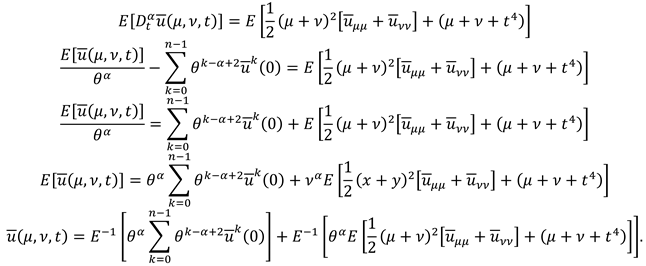
E u _ μ , ν , t θ α k = 0 n 1 θ k α + 2 u _ k ( 0 ) = E u _ μ μ μ , ν , t + u _ ν ν μ , ν , t + f μ , ν , t
E u _ μ , ν , t θ α = k = 0 n 1 θ k α + 2 u _ k ( 0 ) + E u _ μ μ μ , ν , t + u _ ν ν μ , ν , t + f μ , ν , t
E u _ μ , ν , t = θ α k = 0 n 1 θ k α + 2 u _ k ( 0 ) + θ α E u _ μ μ μ , ν , t + u _ ν ν μ , ν , t + f μ , ν , t
u _ μ , ν , t = E 1 θ α k = 0 n 1 θ k α + 2 u _ k 0 + E 1 θ α E u _ μ μ μ , ν , t + u _ ν ν μ , ν , t + f μ , ν , t
Applying HPM:
n = 0 p n u _ n μ , ν , t = E 1 θ α k = 0 n 1 θ k α + 2 u _ k 0
+ p E 1 θ α E n = 0 p n u _ n μ , ν , t μ μ + n = 0 p n u _ n μ , ν , t ν ν + f μ , ν , t
Comparing p 0 :
u _ 0 μ , ν , t = E 1 θ α k = 0 n 1 θ k α + 2 u _ k 0 .           )
Comparing p 1 :
u _ 1 μ , ν , t = E 1 θ α E u _ 0 μ , ν , t μ μ + u _ 0 μ , ν , t ν ν + f μ , ν , t .           )
Comparing p 2 :
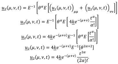
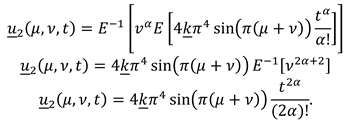
u _ 2 μ , ν , t = E 1 θ α E u _ 1 μ , ν , t μ μ + u _ 1 μ , ν , t ν ν .
Comparing p 3 :
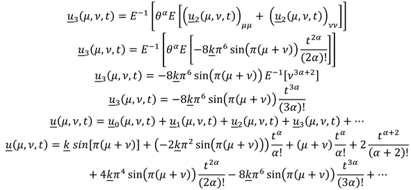
u _ 3 μ , ν , t = E 1 θ α E u _ 2 μ , ν , t μ μ + u _ 2 μ , ν , t ν ν .
Comparing p n :
u _ n μ , ν , t = E 1 θ α E u _ n 1 μ , ν , t μ μ + u _ n 1 μ , ν , t ν ν .
u _ μ , ν , t = u _ 0 μ , ν , t + u _ 1 μ , ν , t + u _ 2 μ , ν , t + + u _ 3 μ , ν , t .

4.2. Methodology for Upper bound solution

Applying Elzaki transform upon Equation (3):
E D t α u ¯ μ , ν , t = E u ¯ μ μ μ , ν , t + u ¯ ν ν μ , ν , t + f μ , ν , t
E u ¯ μ , ν , t θ α k = 0 n 1 θ k α + 2 u ¯ k ( 0 ) = E u ¯ μ μ μ , ν , t + u ¯ ν ν μ , ν , t + f μ , ν , t
E u ¯ μ , ν , t θ α = k = 0 n 1 θ k α + 2 u ¯ k ( 0 ) + E u ¯ μ μ μ , ν , t + u ¯ ν ν μ , ν , t + f μ , ν , t
E u ¯ μ , ν , t = θ α k = 0 n 1 θ k α + 2 u ¯ k ( 0 ) + θ α E u ¯ μ μ μ , ν , t + u ¯ ν ν μ , ν , t + f μ , ν , t
u ¯ μ , ν , t = E 1 θ α k = 0 n 1 θ k α + 2 u ¯ k 0 + E 1 θ α E u ¯ μ μ μ , ν , t + u ¯ ν ν μ , ν , t + f μ , ν , t .
Applying HPM:
n = 0 p n u ¯ n μ , ν , t = E 1 θ α k = 0 n 1 θ k α + 2 u ¯ k 0 + p E 1 θ α E n = 0 p n u ¯ n μ , ν , t μ μ + n = 0 p n u ¯ n μ , ν , t ν ν + f μ , ν , t .
Comparing p 0 :
u ¯ 0 μ , ν , t = E 1 θ α k = 0 n 1 θ k α + 2 u ¯ k 0 .
Comparing p 1 :
u ¯ 1 μ , ν , t = E 1 θ α E u ¯ 0 μ , ν , t μ μ + u ¯ 0 μ , ν , t ν ν + f μ , ν , t .           )
Comparing p 2 :
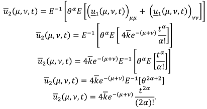
u ¯ 2 μ , ν , t = E 1 θ α E u ¯ 1 μ , ν , t μ μ + u ¯ 1 μ , ν , t ν ν .
Comparing p 3 :
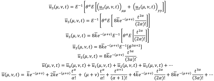
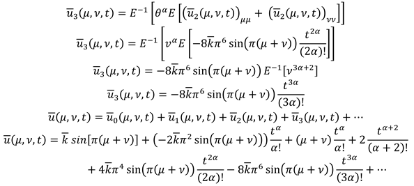
u ¯ 3 μ , ν , t = E 1 θ α E u ¯ 2 μ , ν , t μ μ + u ¯ 2 μ , ν , t ν ν .           )
Comparing p n :
u ¯ n μ , ν , t = E 1 θ α E u ¯ n 1 μ , ν , t μ μ + u ¯ n 1 μ , ν , t ν ν .
u ¯ μ , ν , t = u ¯ 0 μ , ν , t + u ¯ 1 μ , ν , t + u ¯ 2 μ , ν , t + u ¯ 3 μ , ν , t + + u ¯ n μ , ν , t .

5. Existence and Uniqueness

Theorem 1.
Let X be a Banach space and let θ m _ ( x ,   α 1 ) and θ n _ ( x ,   α 1 ) be in X . Suppose γ ( 0 ,   1 ) , then the series solution θ m _ ( x ,   α 1 ) m = 0 which is defined converges to the lower bound solution whenever θ m _ x ,   α 1 γ   θ m 1 _ ( x ,   α 1 ) ,   m > N , that is for any given ε > 0 , there exists a positive number N , such that | | θ m + n _ x , α 1 | | ϵ ,   m ,   n > N   .
Proof. 
Provided
M 0 x , α 1 = θ 0 _ ( x , α 1 )
M 1 x , α 1 = θ 0 _ x ,   α 1 + θ 1 _ ( x ,   α 1 )
M 2 x , α 1 = θ 0 _ x ,   α 1 + θ 1 _ x ,   α 1 + θ 2 _ ( x ,   α 1 )
M 3 x , α 1 = θ 0 _ x ,   α 1 + θ 1 _ x ,   α 1 + θ 2 _ ( x ,   α 1 ) + θ 3 _ ( x ,   α 1 )
M m x , α 1 = θ 0 _ x ,   α 1 + θ 1 _ x ,   α 1 + θ 2 _ x ,   α 1 + θ 3 _ x ,   α 1 + + θ m _ x ,   α 1 .
The aim is to prove that M m x , α 1 is a Cauchy sequence in the Banach space.
It is provided that for γ ( 0,1 )
| | M m + 1 x ,   α 1 M m x ,   α 1 | | = | | θ m + 1 _ x ,   α 1 | |
γ | | θ m _ x ,   α 1 | |
γ 2 | | θ m 1 _ x ,   α 1 | |
γ 3 | | θ m 2 _ x ,   α 1 | |
γ m + 1 | | θ 0 _ x ,   α 1 | | .           )
Let us find Preprints 84942 i006
Considered ϵ = 1 γ ( 1 γ m n ) γ n + 1 | | θ 0 _ x , α 1 | | Preprints 84942 i007is a Cauchy sequence.
Theorem 2.
Let X be a Banach space and let θ m ¯ x ,   α 1 and θ n ¯ x ,   α 1 be in X . Suppose γ ( 0 ,   1 ) , then the series solution θ m ¯ x ,   α 1 m = 0 which is defined m = 0 θ m ¯ x ,   α 1 converges to the upper bound solution whenever θ m ¯ x ,   α 1 γ θ m 1 ¯ x ,   α 1 ,   m > N , that is for any given ε > 0 , there exists a positive number N , such that | | θ m + n ¯ x ,   α 1 | | ϵ ,   m ,   n > N   .
Proof. 
Provided
Preprints 84942 i008
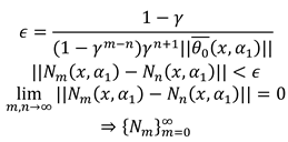
Aim is to prove that N m x , α 1 is a Cauchy sequence. In the Banach space.It is provided that for γ ( 0,1 ) Preprints 84942 i009
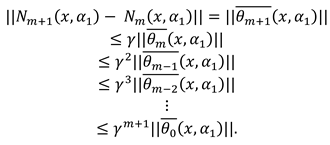
Let find
Preprints 84942 i010
Considered
Preprints 84942 i011
is a Cauchy sequence.
Theorem 3.
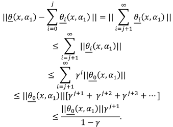
Let i = 0 j θ i _ x ,   α 1 be finite and θ i _ x ,   α 1 be its approximate solution. Suppose γ > 0 , such that || θ i + 1 _ x ,   α 1 | | γ | | θ i _ x ,   α 1 | | ,   γ 0,1 ,   i , then the maximum absolute error for the lower bound solution is
Preprints 84942 i012
Proof. 
Let i = 0 j θ i _ x , α 1 <
Preprints 84942 i013
Theorem 4.
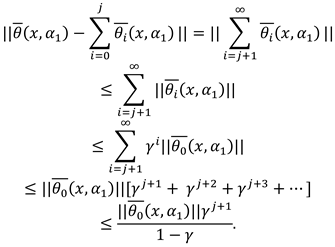
Let i = 0 j θ i ¯ x ,   α 1 be finite and θ i ¯ x ,   α 1 be its approximate solution. Suppose γ > 0 , such that || θ i + 1 ¯ x ,   α 1 | | γ | | θ i ¯ x ,   α 1 | | ,   γ 0,1 ,   i , then the maximum absolute error for the upper bound solution is
Preprints 84942 i014
Proof. 
Let i = 0 j θ i ¯ x , α 1 < , then
Preprints 84942 i015

6. Numerical examples

In the present section, three numerical examples are considered to validate. For each example, series solutions are provided along with the exact solution. It is noted that the series solution converges rapidly towards the exact solution.
Example 1 [32] Preprints 84942 i016 where k ~ = k _ , k ¯ = [ r 1 , 1 r ]

6.1.1. Solution regarding lower bound:

Given Preprints 84942 i017where k ¯ = r − 1.
From developed methodology for lower bound solution:
Comparing p0:
Preprints 84942 i018
Considered n = 1:
Preprints 84942 i019
Comparing p1:
Preprints 84942 i020
Comparing p2:
Preprints 84942 i021
Comparing p3:
Preprints 84942 i022
Remark: 
If f(μ,ν,t) = 0
Preprints 84942 i023

6.1.2. Solution regarding upper bound:

Given
D t α u ¯ ( μ , ν , t ) = u ¯ μ μ ( μ , ν , t ) +   u ¯ ν ν ( μ , ν , t ) + ( μ + ν + t ) u ¯ ( μ , ν , 0 ) = k ¯ e ( x + y )
where k ¯ = 1 − r
From developed methodology for upper bound solution:
Comparing p0:
u ¯ 0 ( μ , ν , t ) = E 1 [ θ α k = 0 n 1 θ k α + 2 u ¯ k ( 0 ) ] .
Considered n = 1:
Preprints 84942 i024
Comparing p1:
Preprints 84942 i025
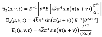
Comparing p2:
Preprints 84942 i026
Comparing p3:
Preprints 84942 i027
Remark: 
If f(μ,ν,t) = 0
Preprints 84942 i028
Example 2 [32]:
D t α u ˜ ( μ , ν , t ) = u ˜ μ μ ( μ , ν , t ) +   u ˜ ν ν ( μ , ν , t ) + ( x + y + t 2 ) u ˜ ( μ , ν , 0 ) = k ˜   s i n [ π ( μ + ν ) ] ,   k ˜ = [ k _ ( r ) ,   k ¯ ( r ) ] = [ r 1 ,   1 r ]

6.2.1. Regarding lower bound solution:

D t α u _ ( μ , ν , t ) = u _ μ μ ( μ , ν , t ) +   u _ ν ν ( μ , ν , t ) + ( μ + ν + t 2 ) u _ ( μ , ν , 0 ) = k _   s i n [ π ( μ + ν ) ] ,   k _ = r 1
From the methodology regarding Lower bound solution:
Comparing p0:
u _ 0 ( μ , ν , t ) = E 1 [ θ α k = 0 n 1 θ k α + 2 u _ k ( 0 ) ]
Comparing n = 1:
u _ 0 ( μ , ν , t ) = E 1 [ θ 2 u _ ( 0 ) ] u _ 0 ( μ , ν , t ) = u _ ( 0 ) = k _   s i n [ π ( μ + ν ) ]
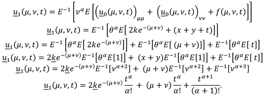
Comparing p1:
Preprints 84942 i029
Comparing p2:
Preprints 84942 i030
Comparing p3:
Preprints 84942 i031
Remark: 
If f(x,y,t) = 0
Preprints 84942 i032

6.2.2. Regarding upper bound solution:

D t α u ¯ ( μ , ν , t ) = u ¯ μ μ ( μ , ν , t ) +   u ¯ ν ν ( μ , ν , t ) + ( μ + ν + t 2 ) u ¯ ( μ , ν , 0 ) = k ¯   s i n [ π ( μ + ν ) ] ,   k ¯ = 1 r .
From the methodology regarding Upper bound solution:
Comparing p0:
u ¯ 0 ( μ , ν , t ) = E 1 [ θ α k = 0 n 1 θ k α + 2 u ¯ k ( 0 ) ] .
Considered n = 1:
Preprints 84942 i033
Comparing p1:
Preprints 84942 i034
Comparing p2:
Preprints 84942 i035
Comparing p3:
Preprints 84942 i036
Remark: 
If f(x,y,t) = 0
Preprints 84942 i037
Example 3 [32] :
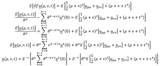
D t α u ˜ ( μ , ν , t ) = 1 2 ( x + y ) 2 [ u ˜ μ μ + u ˜ ν ν ] + ( μ + ν + t 4 ) u ˜ ( μ , ν , 0 ) = k ˜ ( μ + ν ) 2 , k ˜ = [ k _ ( r ) ,   k ¯ ( r ) ] = [ r 1 ,   1 r ] .

6.3.1. Regarding Lower bound solution:

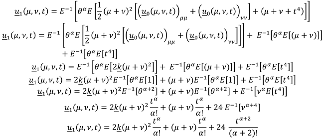
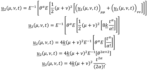
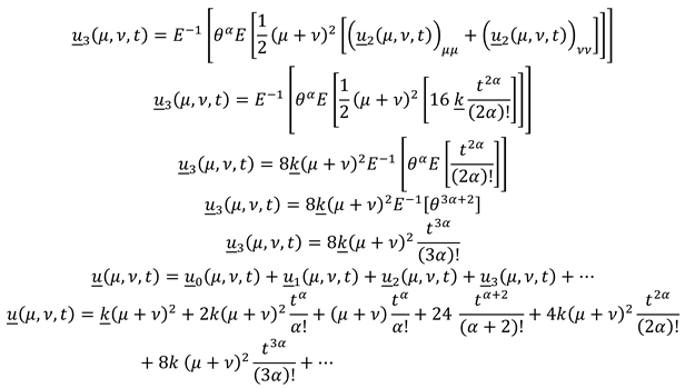
D t α u _ ( μ , ν , t ) = 1 2 ( μ + ν ) 2 [ u _ μ μ + u _ ν ν ] + ( μ + ν + t 4 )
I.C.: u _ ( μ , ν , 0 ) = k _ ( μ + ν ) 2 , k _ = r 1
Applying Elzaki transform:
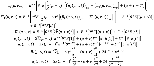
Preprints 84942 i038
Applying HPM:
Preprints 84942 i039
Comparing p0:
Preprints 84942 i040
Comparing p1:
Preprints 84942 i041
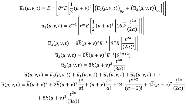
Comparing p2:
Preprints 84942 i042
Comparing p3:
Preprints 84942 i043
Remark:
If f(μ,ν,t) = 0:
Preprints 84942 i044

6.3.2. Regarding upper bound solution:

Preprints 84942 i045
Applying Elzaki transform:
Preprints 84942 i046
ApplyingHPM:
Preprints 84942 i047
Comparing p0:
Preprints 84942 i058Preprints 84942 i059
Comparing p1:
Preprints 84942 i048
Comparing p2:
Preprints 84942 i048
Comparing p3:
Preprints 84942 i050
Remark:
If f(μ,ν,t) = 0:
Preprints 84942 i051

7. Results and discussion

Remark 1.
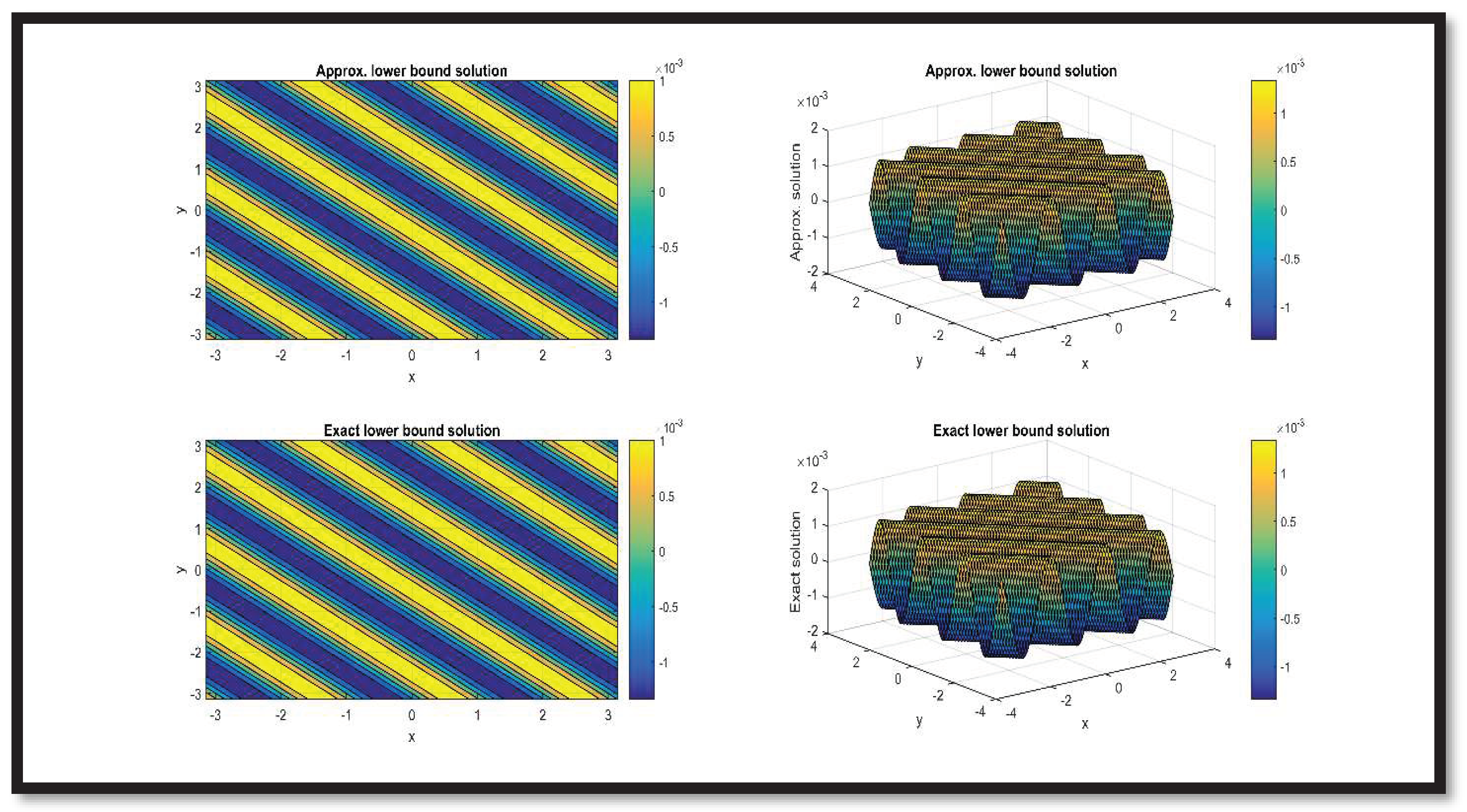
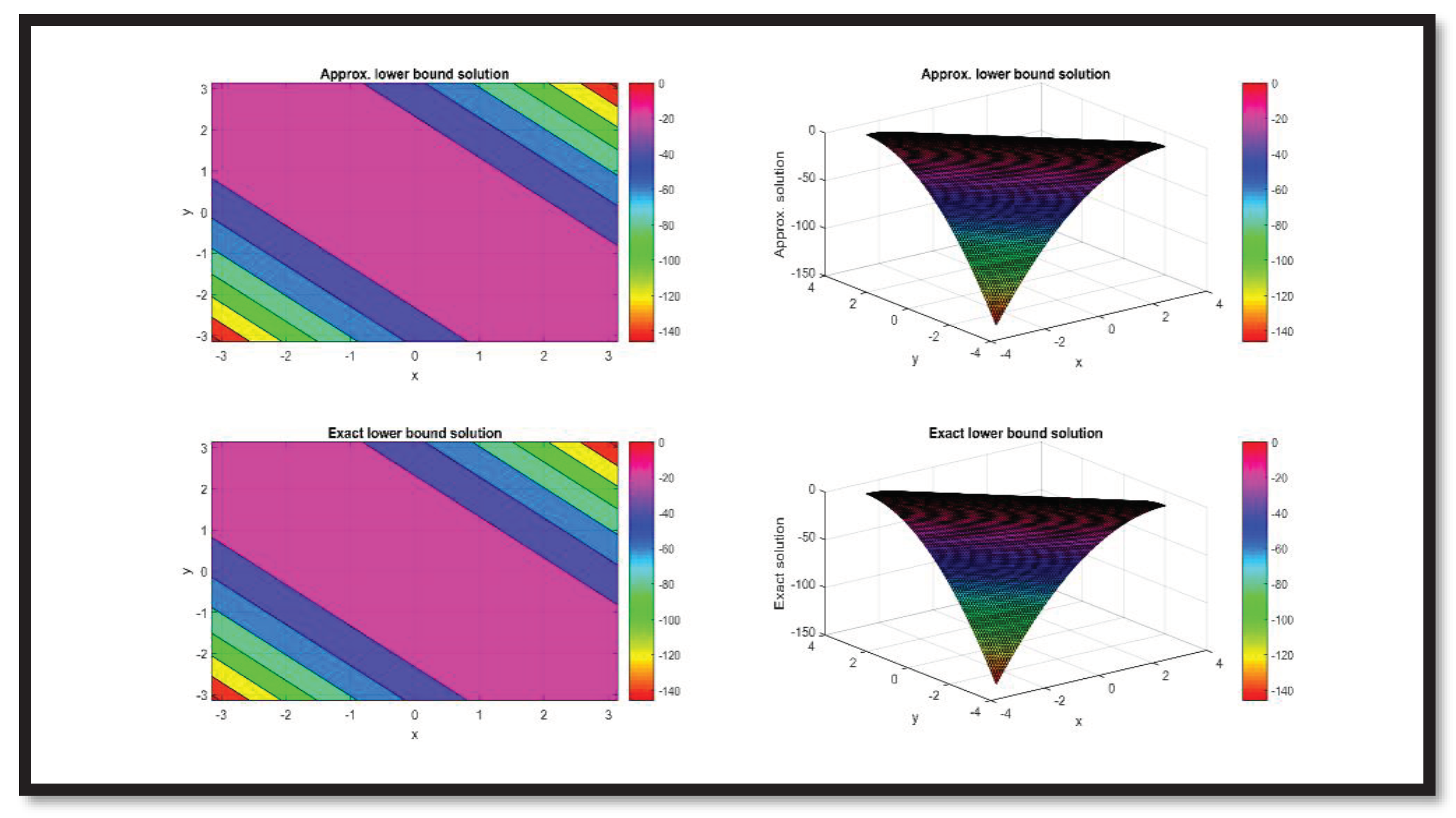
In Figure 1, the contour and surface graphs are matched for approximated and exact lower bound solutions at t = 1.
Remark 2.
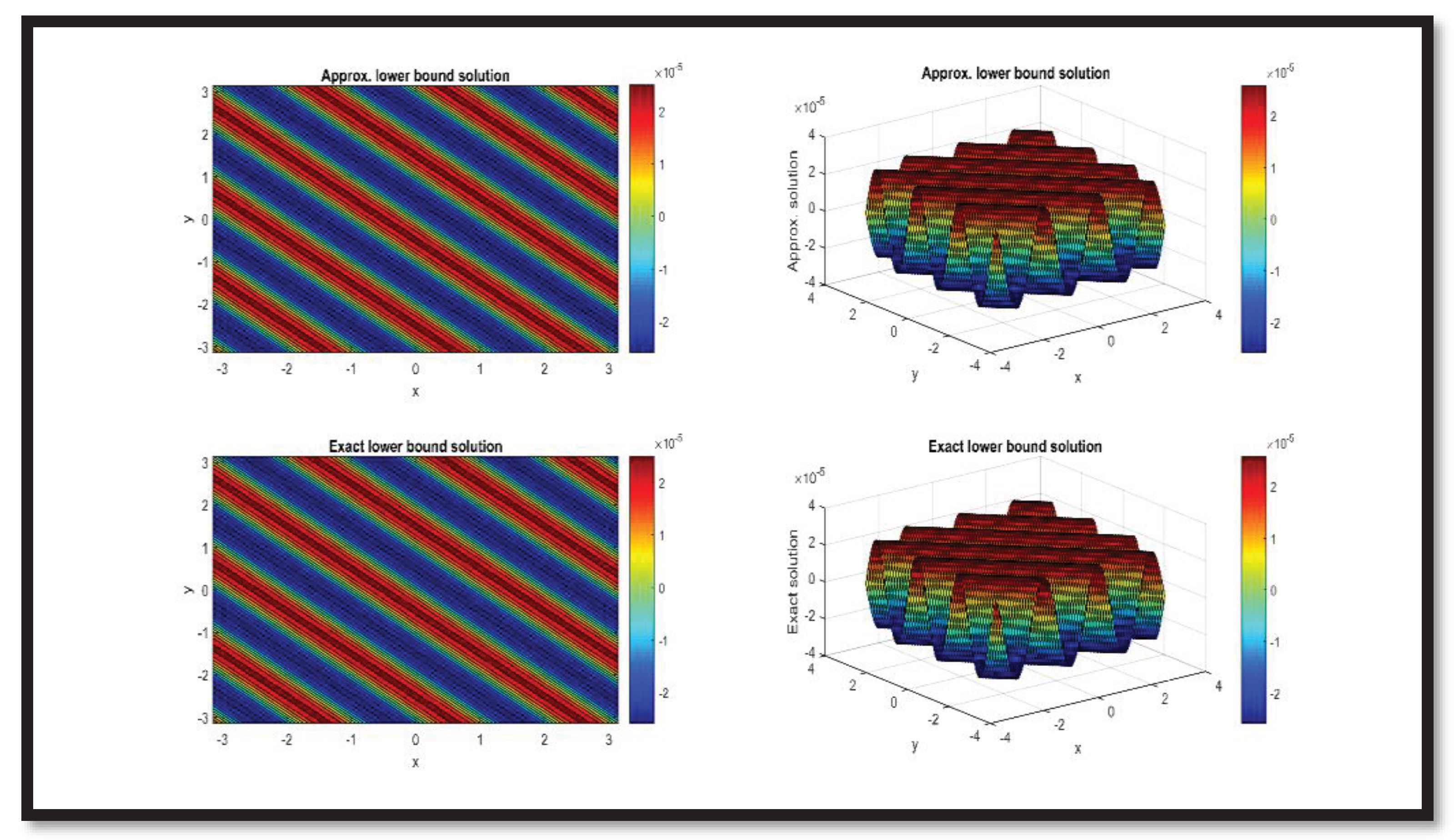
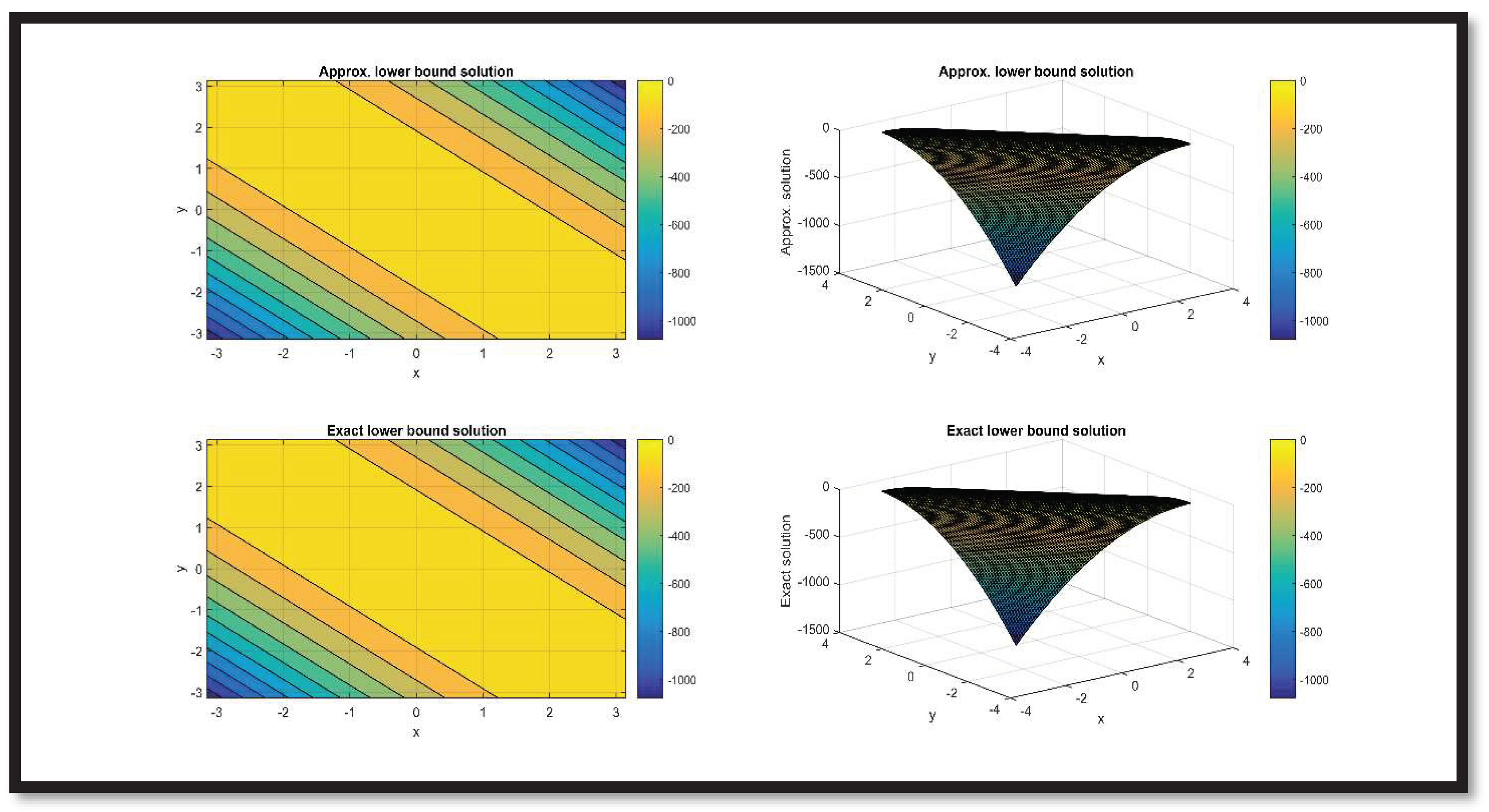
In Figure 2, the contour and surface graphs are matched for approximated and exact lower bound solutions at t = 2.
Remark 3.
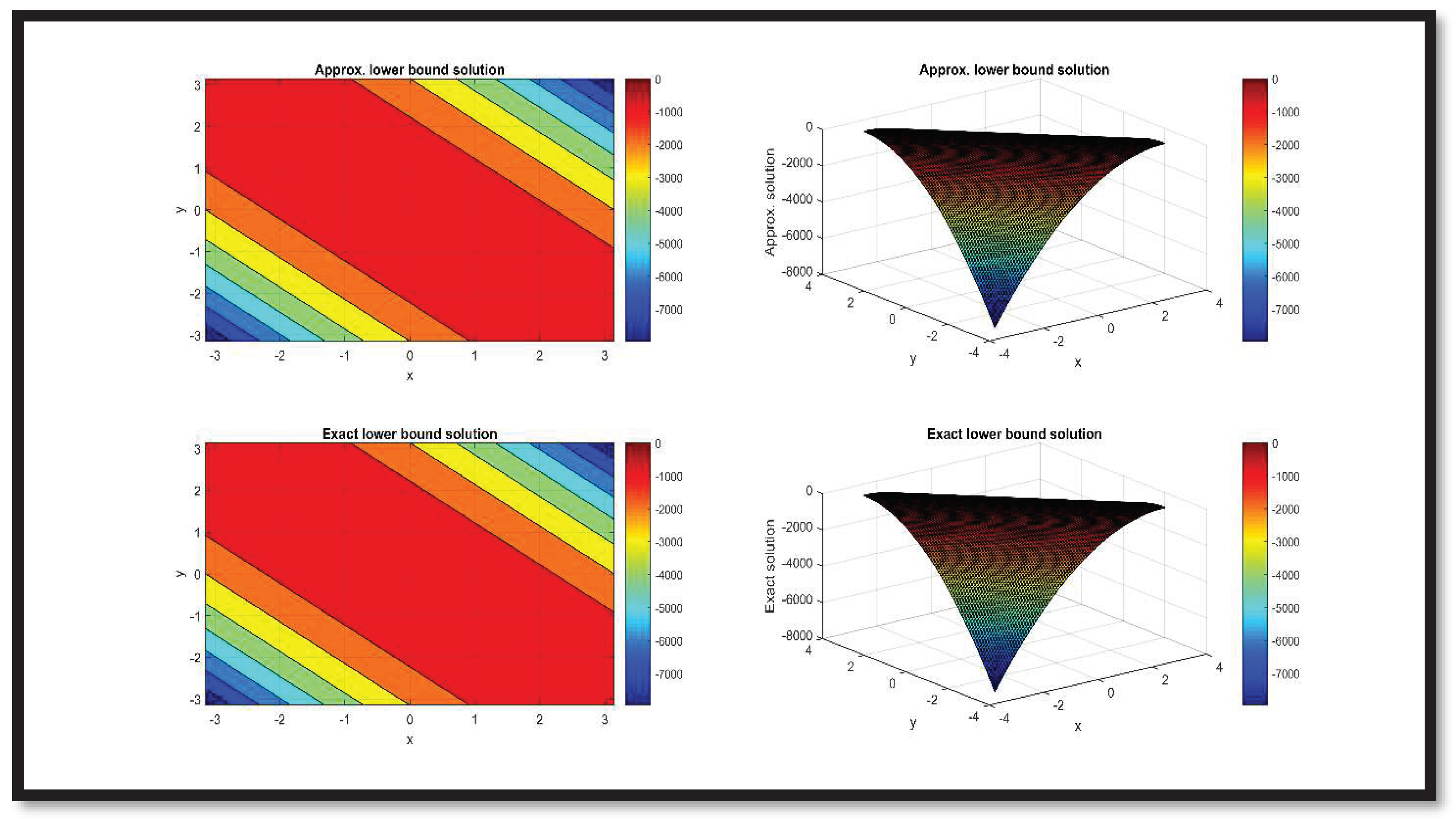
In Figure 3, the contour and surface graphs are matched for approximated and exact lower bound solutions at t = 3.
Remark 4.
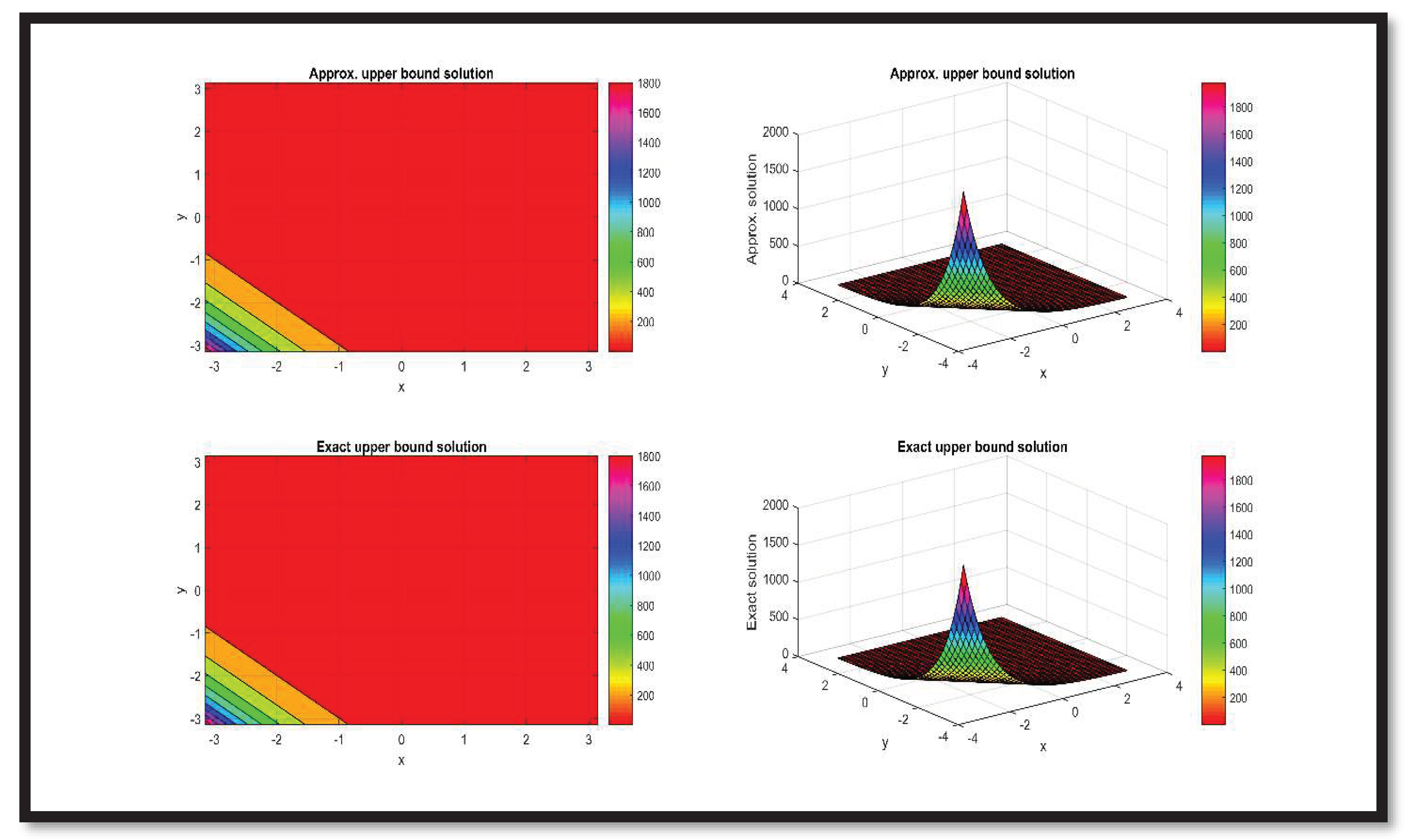
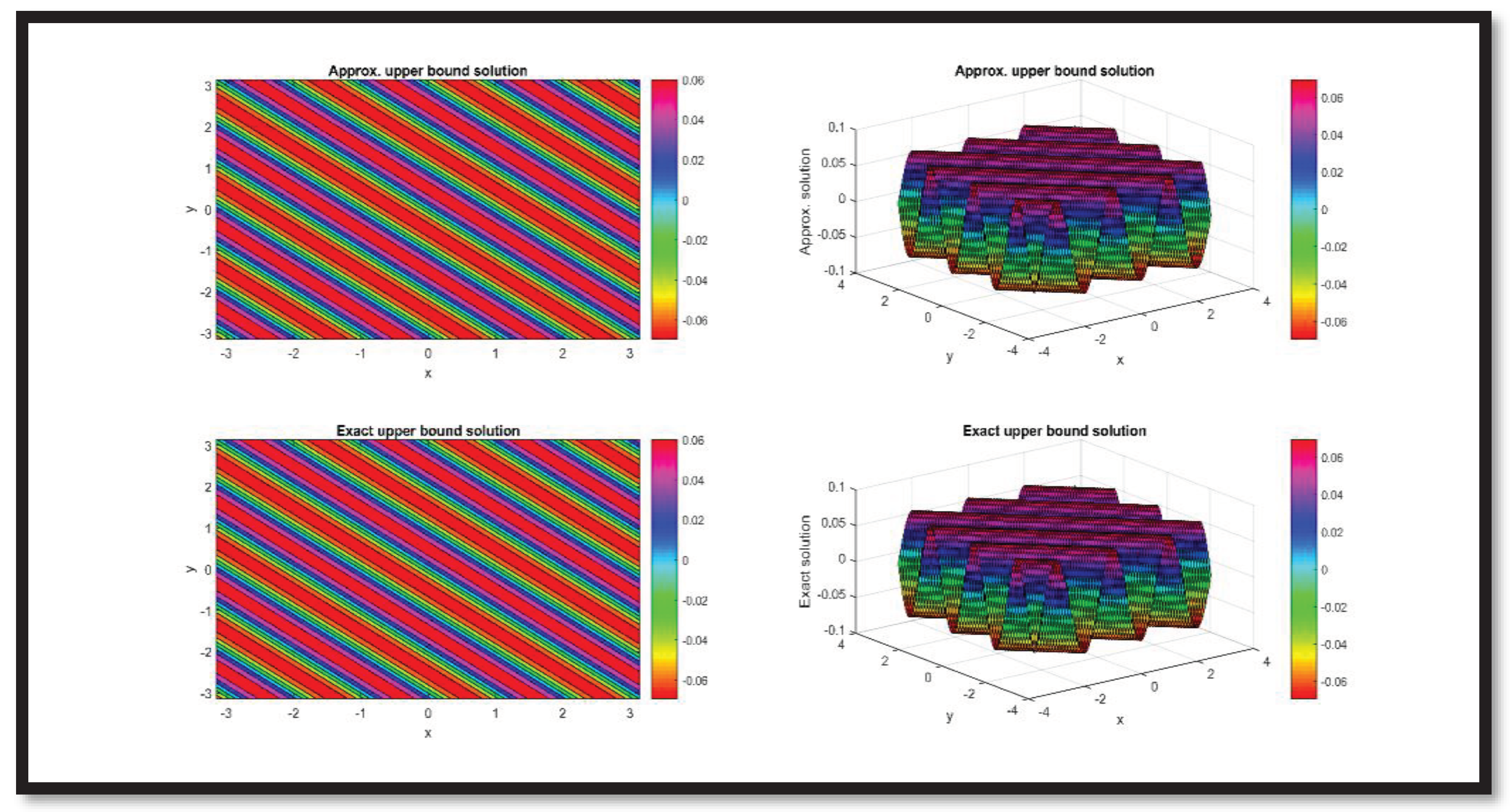
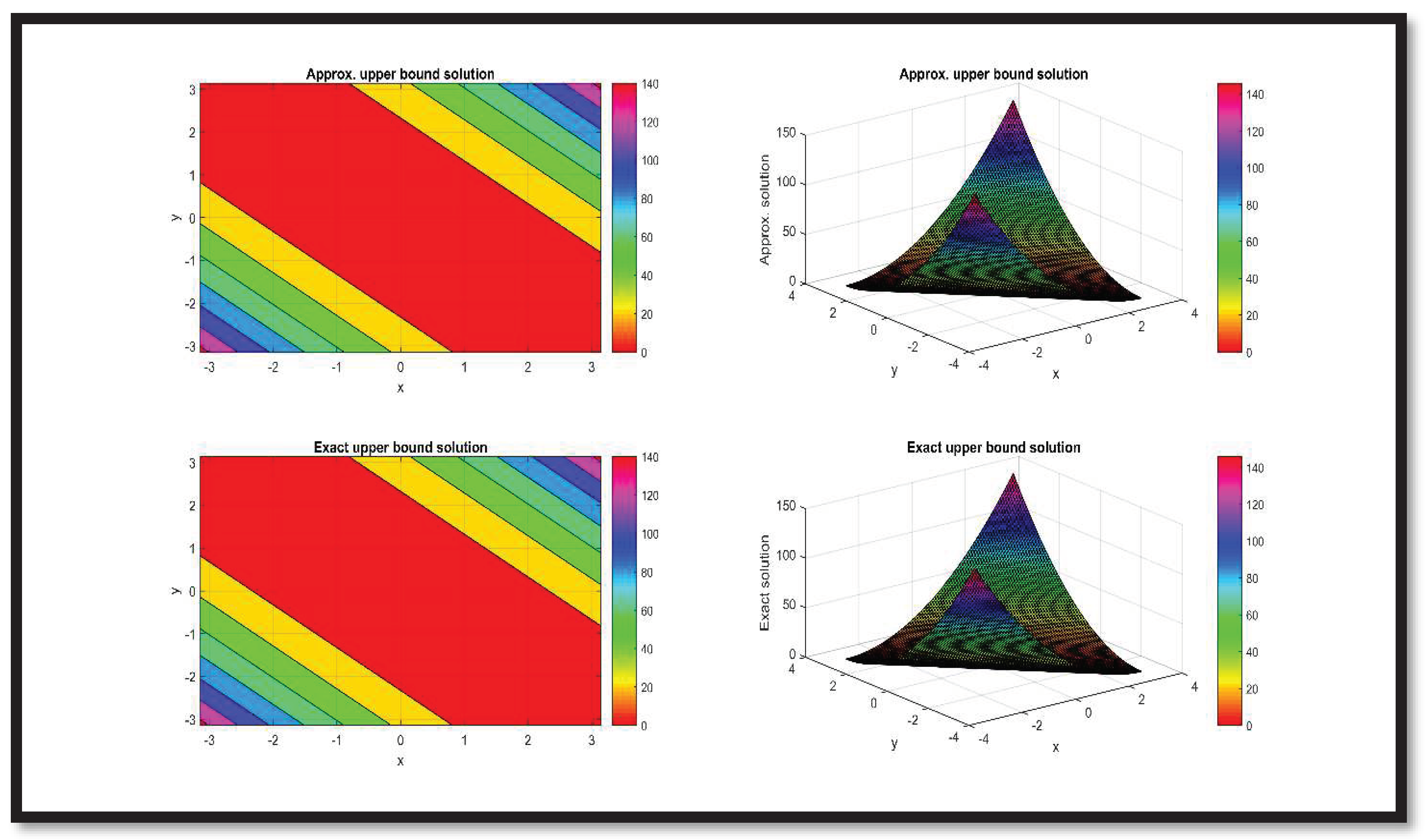
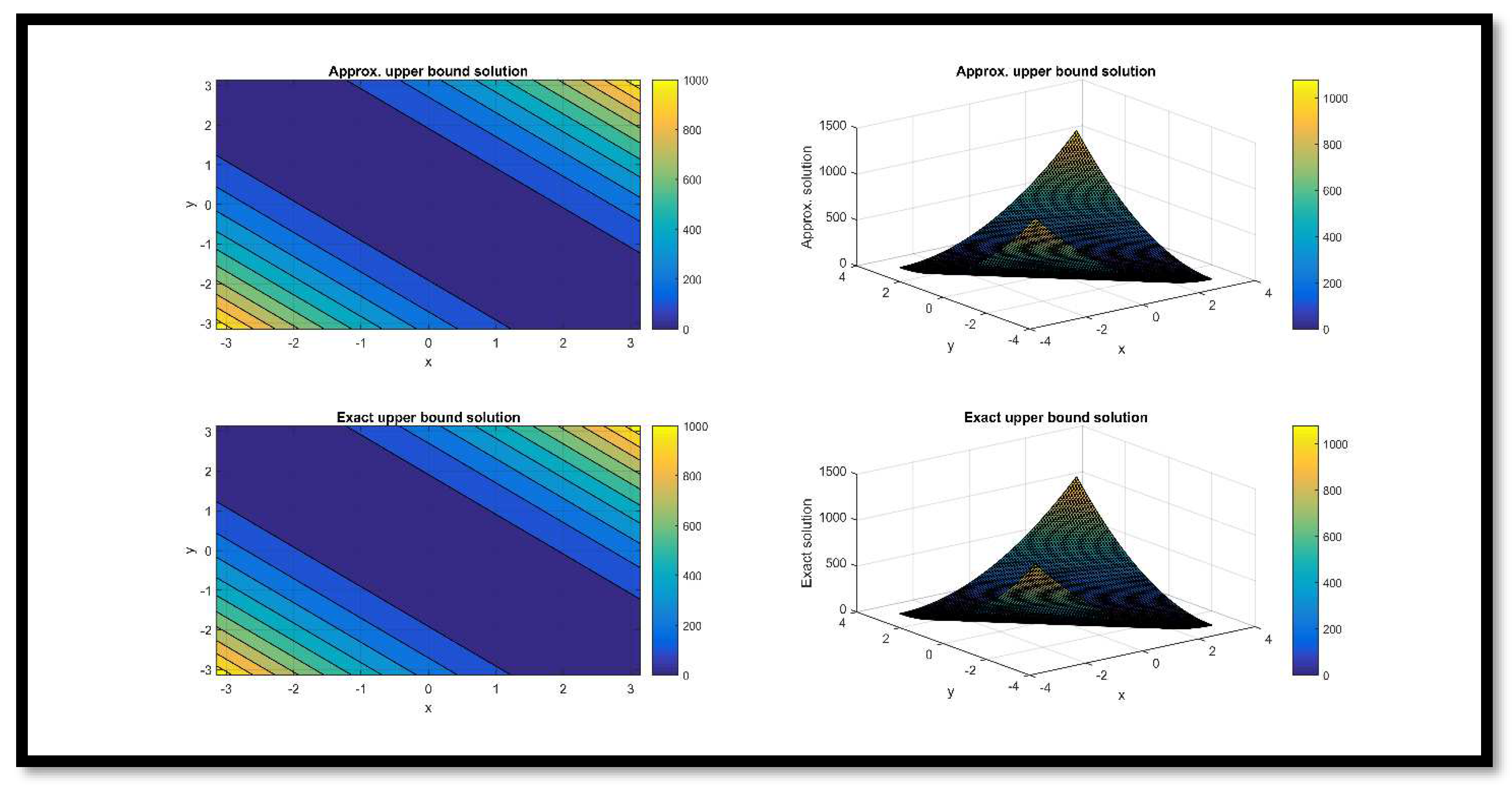
In Figure 4, the contour and surface graphs are matched for approximated and exact upper bound solutions at t = 1.
Remark 5.
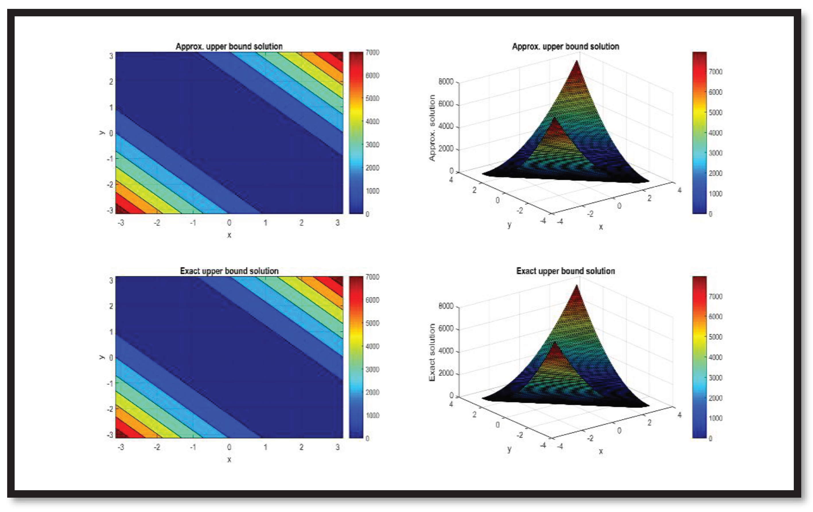
In Figure 5, the contour and surface graphs are matched for approximated and exact upper bound solutions at t = 2.
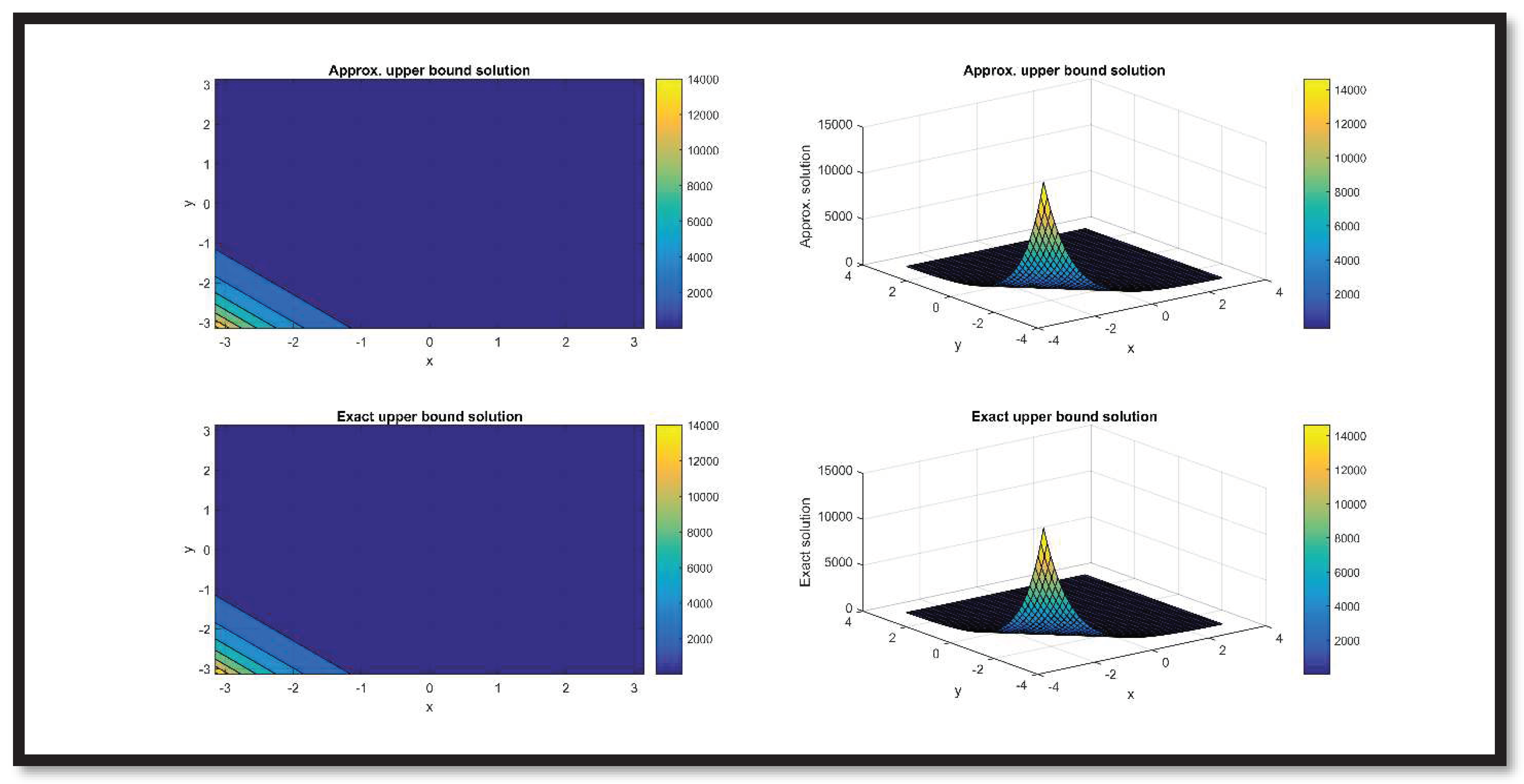
Remark 6.
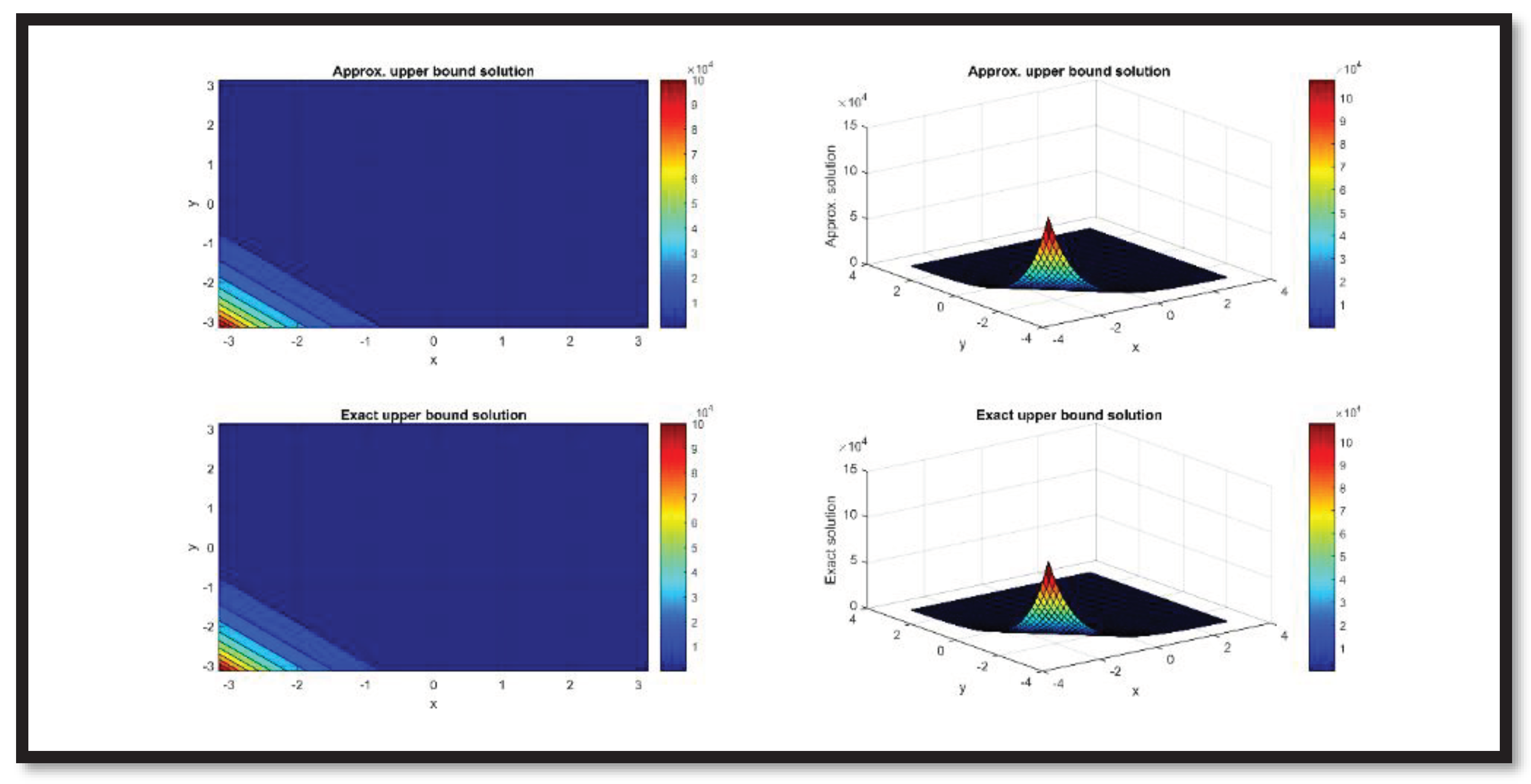
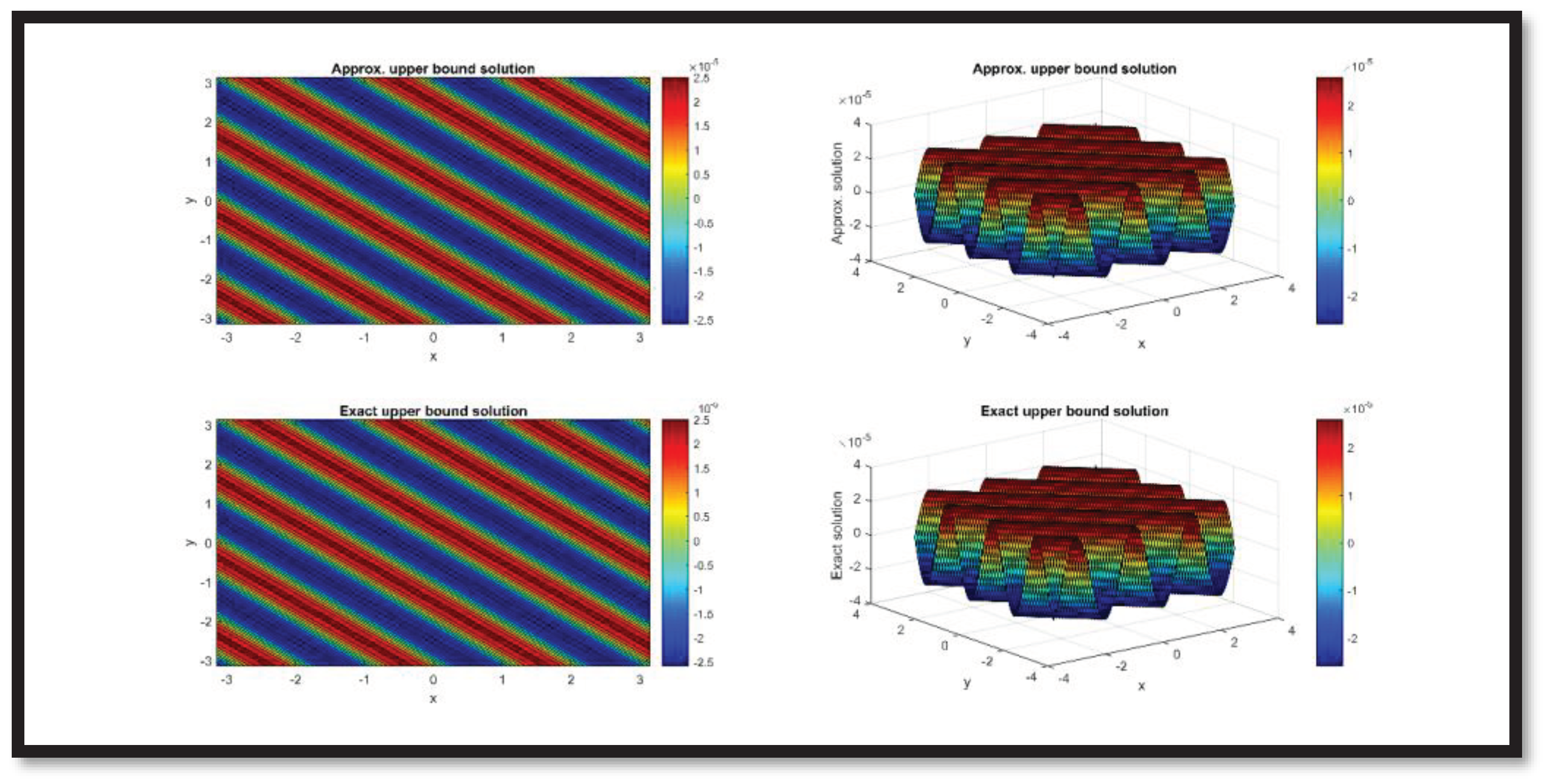
In Figure 6, the contour and surface graphs are matched for approximated and exact upper bound solutions at t = 3.
Remark 7.
In Table 2, L error for lower bound is provided at t = 0.5, 0.8 and 1.0.
Remark 8.
In Table 3, L error for upper bound is provided at t = 0.5, 0.8 and 1.0 respectively.
Remark 9.
In Table 4. Approximated and exact lower bound solutions are matched at t = 0.5 and 1.0 respectively.
Remark 10.
In Table 5. Approximated and exact upper bound solutions are matched at t = 0.5 and 1.0 respectively.
Remark 11.
In Figure 7, contour and surface graphs of lower bound solution are provided at t = 0.1.
Remark 12.
In Figure 8, contour and surface graphs of lower bound solution are provided at t = 0.3.
Remark 13.
In Figure 9, contour and surface graphs of the lower bound solution are provided at t = 0.5.
Remark 14.
In Figure 10, contour and surface graphs of the upper bound solution are provided at t = 0.1.
Remark 15.
In Figure 11, contour and surface graphs of the upper bound solution are provided at t = 0.3.
Remark 15.
In Figure 12, contour and surface graphs of the upper bound solution are provided at t = 0.5.
Remark 16.
In Table 6, L error for lower and upper bound solutions is provided at t = 0.5.
Remark 17.
In Table 7, L error for lower and upper bound solutions is provided at t = 0.8.
Remark 18.
In Table 8, L error for lower and upper bound solutions is provided at t = 1.0.
Remark 19.
In Table 9, a comparison of approximated and exact solutions is provided for the lower bound at t = 0.1 and 0.2, along with the absolute error.
Remark 20.
In Table 10, a comparison of approximated and exact solutions is provided for the upper bound at t = 0.1 and 0.2, along with the absolute error.
Remark 21.
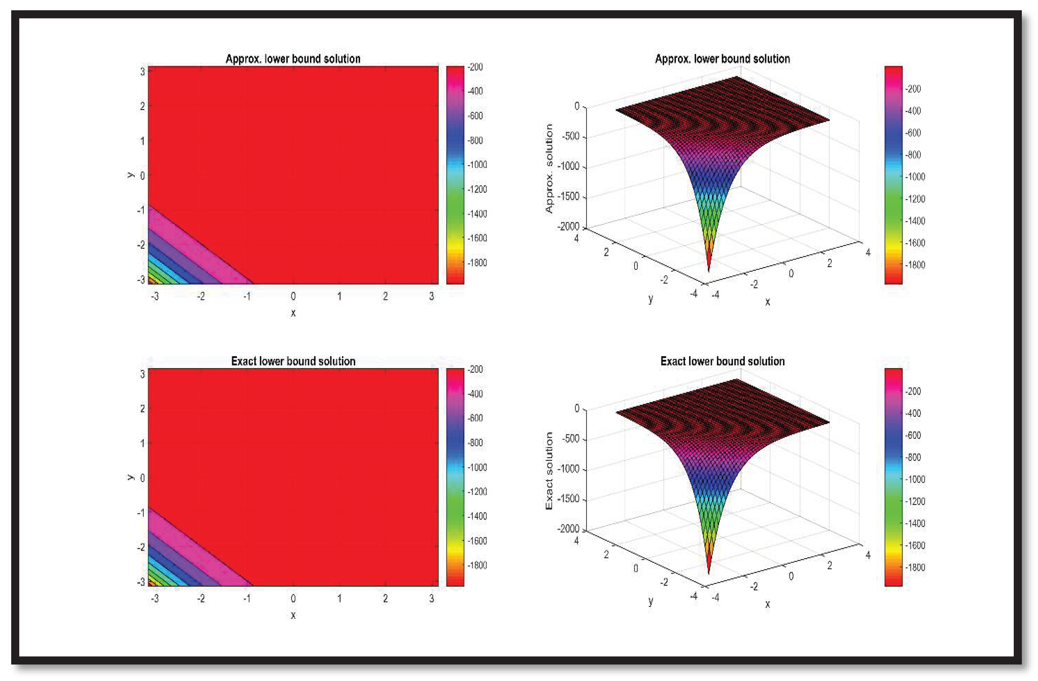
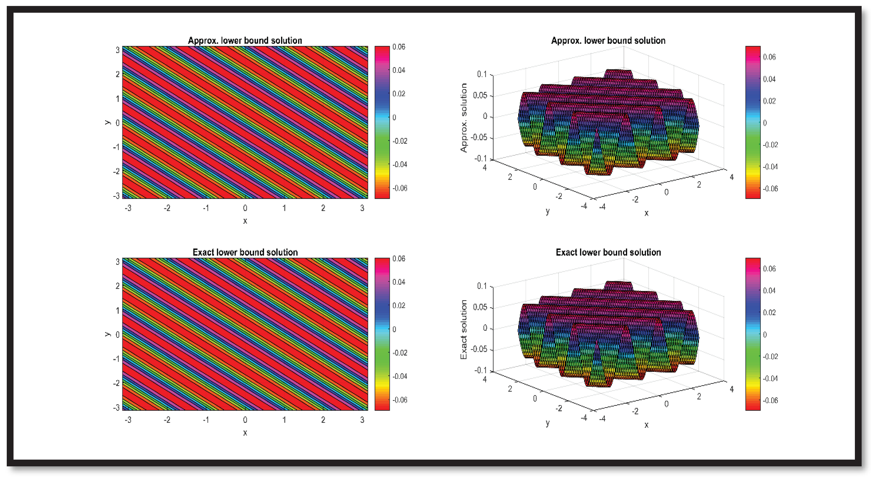
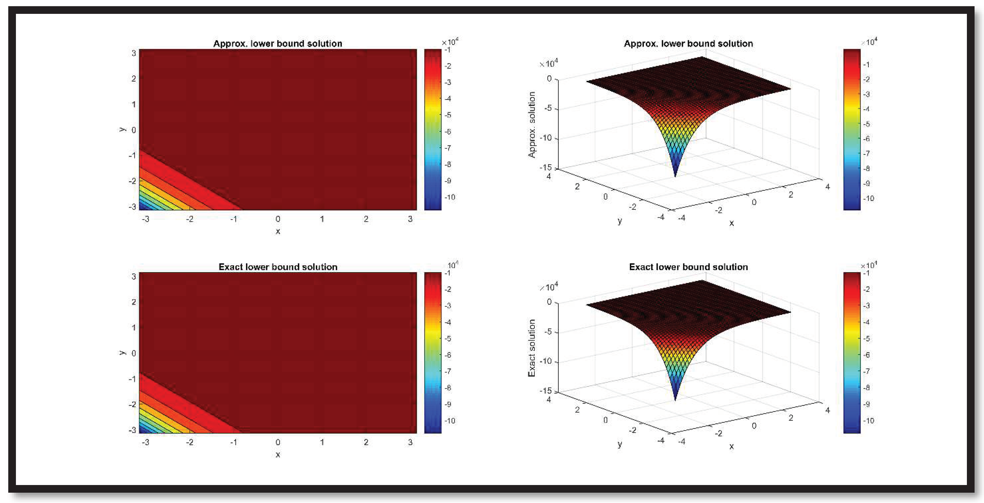
In Figure 13, a comparison of approximated and exact lower bound solutions is provided at t = 1.
Remark 22.
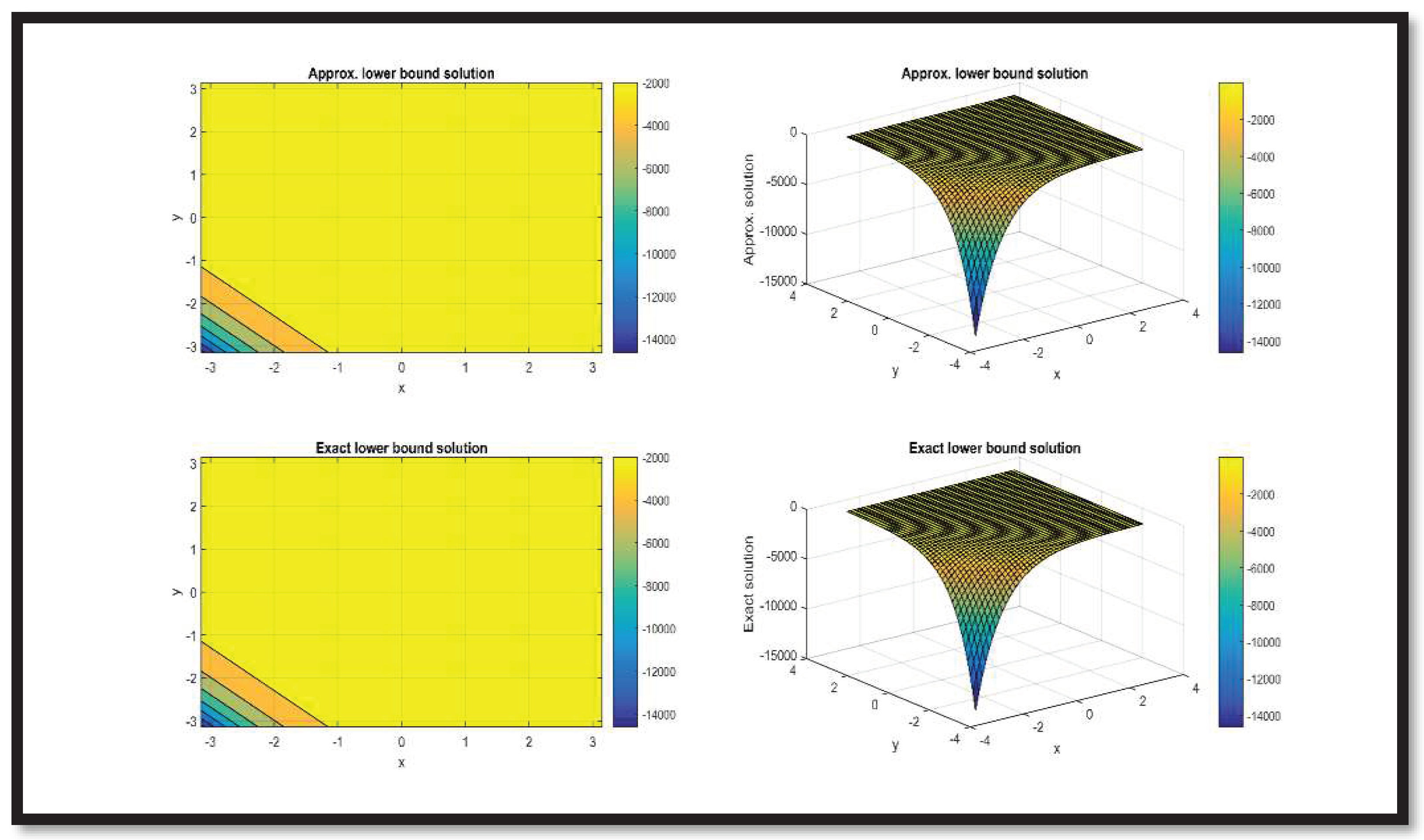
In Figure 14, a comparison of approximated and exact lower bound solutions is provided at t = 2.
Remark 23.
In Figure 15, a comparison of approximated and exact lower bound solutions is provided at t = 3.
Remark 24.
In Figure 16, a comparison of approximated and exact upper bound solutions is provided at t = 1.
Remark 25.
In Figure 17, a comparison of approximated and exact upper bound solutions is provided at t = 2.
Remark 26:
In Figure 18, a comparison of approximated and exact upper bound solutions is provided at t = 3.
Remark 27:
In Table 11, L error for lower and upper bound solutions is provided at t = 1.0.
Remark 28:
In Table 12, L error for lower and upper bound solutions is provided at t = 2.0.
Remark 29:
In Table 13, L error for lower and upper bound solutions is provided at t = 3.0.
Remark 30.
In Table 14, approximated and exact lower bound solutions are matched at t = 0.5 and t = 1.0 along with absolute error.
Remark 31.
In Table 14, approximated and exact upper bound solutions are matched at t = 0.5 and t = 1.0, along with absolute error.
Table 15. Comparison of Approximated and Exact upper bound solutions at t = 0.5 and t = 1.0 for Example 3.
Preprints 84942 i057

8. Concluding Remarks

The two-dimensional fuzzy fractional Heat equation is studied via a regime named Elzaki HPM. A novel regime is developed via the fusion of the Elzaki transform and the Homotopy Perturbation Method. Three numerical examples are studied in this paper. The compatibility of the approximated and exact results is matched by means of graphs and tables.Via Figure 1Figure 18,the graphical compatibility of the approximated and exact solutions for the lower and upper bound is validated. Via Table 2Table 15, the numerical convergence and matching of approximated and exact solutions are validated. It is affirmed on the basis of all these results that the proposed regime can produce results that converge rapidly to the exact solution.The study conducted in this paper will surely open new dimensions for researchers. This regime will be helpful in studying some higher-order fuzzy fractional partial differential equations such as; the KdV equation, Kawahara equation and Sawada Kotera equation and many others.

Author Contributions

For research articles with several authors, a short paragraph specifying their individual contributions must be provided. The following statements should be used “Conceptualization, Mamta Kapoor, D. G. Prakasha and Nehad Ali Shah; methodology, P. Veeresha and Nasser Bin Turki.; software, mamta Kapoor; validation, Mamta Kapoor, P. Veeresha, Nasser Bin Turki and Nehad Ali Shah; formal analysis, D. G. Prakasha and Nasser Bin Turki; investigation, Mamta Kapoor, P. veeresha, Nehad Ali Sha; resources,Mamta Kapoor, P. Veeresha and Nasser Bin Turki; data curation, P. Veeresha, D. G. Prakasha and Nehad Ali Shah; writing—original draft preparation, Mamta Kapoor, D. G. Prakasha, P. Veeresha, Nasser Bin Turki; writing—review and editing, P. veeresha and Nehad Ali Shah; visualization, Mamta Kapoor; supervision, P. Veeresha and Nasser Bin Turki.; project administration, Nasser Bin Turki.; funding acquisition, Nasser Bin Turki.

Funding

Please This research was funded by King Saud University, Riyadh, Saudi Arabia and grant number RSP2023R413” and “The APC was funded by NBT”.

Conflicts of Interest

The authors declare no conflict of interest.

References

  1. Allahviranloo, T.; Salahshour, S.; Abbasbandy, S. Explicit solutions of fractional differential equations with uncertainty. Soft Comput. 2012, 16, 297–302. [Google Scholar] [CrossRef]
  2. Rahaman, M.; Mondal, S.P.; El Allaoui, A.; Alam, S.; Ahmadian, A.; Salahshour, S. Solution strategy for fuzzy fractional order linear homogeneous differential equation by Caputo-H differentiability and its application in fuzzy EOQ model. Advances in Fuzzy Integral and Differential Equations 2022, 143–157. [Google Scholar]
  3. Choi, H.; Sin, K.; Pak, S.; Sok, K.; So, S. Representation of solution of initial value problem for fuzzy linear multi-term fractional differential equation with continuous variable coefficient. AIMS Math. 2019, 4, 613–625. [Google Scholar] [CrossRef]
  4. Salahshour, S.; Ahmadian, A.; Senu, N.; Baleanu, D.; Agarwal, P. On Analytical Solutions of the Fractional Differential Equation with Uncertainty: Application to the Basset Problem. Entropy 2015, 17, 885–902. [Google Scholar] [CrossRef]
  5. Anastassiou, G.A.; Anastassiou, G.A. Fuzzy fractional calculus and the Ostrowski integral inequality. Intelligent Mathematics: Computational Analysis 2011, 553–574.
  6. Caputo, M.; Fabrizio, M. The Kernel of the Distributed Order Fractional Derivatives with an Application to Complex Materials. Fractal Fract. 2017, 1, 13. [Google Scholar] [CrossRef]
  7. Khan, I. New idea of Atangana and Baleanu fractional derivatives to human blood flow in nanofluids. Chaos: Interdiscip. J. Nonlinear Sci. 2019, 29, 013121. [Google Scholar] [CrossRef]
  8. Zadeh, L. Fuzzy sets. Inform Control 1965, 8, 338–353. [Google Scholar] [CrossRef]
  9. Klir, G. J., & Yuan, B. (Eds.). (1996). Fuzzy sets, fuzzy logic, and fuzzy systems: selected papers by Lotfi A Zadeh (Vol. 6). World Scientific.
  10. Dubois, D.; Prade, H. Towards fuzzy differential calculus part 1: Integration of fuzzy mappings. Fuzzy Sets Syst. 1982, 8, 1–17. [Google Scholar] [CrossRef]
  11. Goetschel, R., Jr; Voxman, W. Elementary fuzzy calculus. Fuzzy sets and systems 1986, 18, 31–43. [Google Scholar] [CrossRef]
  12. Kaleva, O. Fuzzy differential equations. Fuzzy sets and systems 1987, 24, 301–317. [Google Scholar] [CrossRef]
  13. Wang, L. X. (1996). A course in fuzzy systems and control. Prentice-Hall, Inc.
  14. Kapoor, M.; Shah, N.A.; Saleem, S.; Weera, W. An Analytical Approach for Fractional Hyperbolic Telegraph Equation Using Shehu Transform in One, Two and Three Dimensions. Mathematics 2022, 10, 1961. [Google Scholar] [CrossRef]
  15. Kapoor, M.; Majumder, A.; Joshi, V. An analytical approach for Shehu transform on fractional coupled 1D, 2D and 3D Burgers’ equations. Nonlinear Eng. 2022, 11, 268–297. [Google Scholar] [CrossRef]
  16. Kapoor, M. (2022). Shehu transform on time-fractional Schrödinger equations–an analytical approach. International Journal of Nonlinear Sciences and Numerical Simulation.
  17. Kapoor, M.; Shah, N.A.; Weera, W. Analytical solution of time-fractional Schrödinger equations via Shehu Adomian Decomposition Method. AIMS Math. 2022, 7, 19562–19596. [Google Scholar] [CrossRef]
  18. Kapoor, M.; Khosla, S. Semi-analytical approximation of time-fractional telegraph equation via natural transform in Caputo derivative. Nonlinear Eng. 2023, 12. [Google Scholar] [CrossRef]
  19. Kapoor, M.; Joshi, V. A comparative study of Sumudu HPM and Elzaki HPM for coupled Burgers’ equation. Heliyon 2023, 9, e15726. [Google Scholar] [CrossRef]
  20. Elzaki, T.M.; Hilal, E.M.; Arabia, J.-S.; Arabia, J.-S. Homotopy perturbation and Elzaki transform for solving nonlinear partial differential equations. Math. Theory Model. 2012, 2, 33–42. [Google Scholar]
  21. He, J.-H. Homotopy perturbation technique. Comput. Methods Appl. Mech. Eng. 1999, 178, 257–262. [Google Scholar] [CrossRef]
  22. He, J.-H. Homotopy perturbation method: a new nonlinear analytical technique. Appl. Math. Comput. 2003, 135, 73–79. [Google Scholar] [CrossRef]
  23. He, J.-H. Application of homotopy perturbation method to nonlinear wave equations. Chaos, Solitons Fractals 2005, 26, 695–700. [Google Scholar] [CrossRef]
  24. Bhadane, P.K.G.; Pradhan, V. Elzaki transform homotopy perturbation method for solving gas dynamics Equation. Int. J. Res. Eng. Technol. 2013, 2, 260–264. [Google Scholar]
  25. Singh, P.; Sharma, D. Comparative study of homotopy perturbation transformation with homotopy perturbation Elzaki transform method for solving nonlinear fractional PDE. Nonlinear Eng. 2020, 9, 60–71. [Google Scholar] [CrossRef]
  26. Iqbal, S.; Martínez, F.; Kaabar, M.K.A.; Samei, M.E. A novel Elzaki transform homotopy perturbation method for solving time-fractional non-linear partial differential equations. Bound. Value Probl. 2022, 2022, 1–23. [Google Scholar] [CrossRef]
  27. Chakraverty, S.; Tapaswini, S.; Behera, D. (2016). Fuzzy arbitrary order system: fuzzy fractional differential equations and applications. John Wiley & Sons.
  28. Rashid, S., Ashraf, R., &Hammouch, Z. (2021). New generalized fuzzy transform computations for solving fractional partial differential equations arising in oceanography. Journal of Ocean Engineering and Science.
  29. Kapoor, M.; Joshi, V. Comparison of Two Hybrid Schemes Sumudu HPM and Elzaki HPM for Convection-Diffusion Equation in Two and Three Dimensions. Int. J. Appl. Comput. Math. 2022, 8, 1–24. [Google Scholar] [CrossRef]
  30. Hajira, Khan, H., Khan, A., Kumam, P., Baleanu, D., & Arif, M. (2020). An approximate analytical solution of the Navier–Stokes equations within Caputo operator and Elzaki transform decomposition method. Advances in Difference Equations, 2020(1), 622.
  31. Salah, A.; Khan, M.; Gondal, M.A. A novel solution procedure for fuzzy fractional heat equations by homotopy analysis transform method. Neural Comput. Appl. 2012, 23, 269–271. [Google Scholar] [CrossRef]
  32. Arfan, M.; Shah, K.; Abdeljawad, T.; Hammouch, Z. An efficient tool for solving two-dimensional fuzzy fractional-ordered heat equation. Numerical Methods for Partial Differential Equations 2021, 37, 1407–1418. [Google Scholar] [CrossRef]
Figure 1. Comparison of Approximate and Exact lower bound solutions at t = 1 for Example 1.
Preprints 84942 g001
Figure 2. Comparison of Approximated and Exact lower bound solutions at t = 2 for Example 1.
Preprints 84942 g002
Figure 3. Comparison of Approximated and Exact lower bound solutions at t = 3 for Example 1.
Preprints 84942 g003
Figure 4. Comparison of Approximated and Exact upper bound solutions at t = 1 for Example 1.
Preprints 84942 g004
Figure 5. Comparison of Approximated and Exact upper bound solutions at t = 2 for Example 1.
Preprints 84942 g005
Figure 6. Comparison of Approximated and Exact upper bound solutions at t = 3 for Example 1.
Preprints 84942 g006
Figure 7. Comparison of Approximated and Exact lower bound solutions at t = 0.1 for Example 2.
Preprints 84942 g007
Figure 8. Comparison of Approximated and Exact lower bound solutions at t = 0.3 for Example 2.
Preprints 84942 g008
Figure 9. Comparison of Approximated and Exact lower bound solutions at t = 0.5 for Example 2.
Preprints 84942 g009
Figure 10. Comparison of Approximated and Exact upper bound solutions at t = 0.1 for Example 2.
Preprints 84942 g010
Figure 11. Comparison of Approximated and Exact upper bound solutions at t = 0.3 for Example 2.
Preprints 84942 g011
Figure 12. Comparison of Approximated and Exact upper bound solutions at t = 0.5 for Example 2.
Preprints 84942 g012
Figure 13. Comparison of Approximated and Exact lower bound solutions at t = 1 for Example 3.
Preprints 84942 g013
Figure 14. Comparison of Approximated and Exact lower bound solutions at t = 2 for Example 3.
Preprints 84942 g014
Figure 15. Comparison of Approximated and Exact lower bound solutions at t = 3 for Example 3.
Preprints 84942 g015
Figure 16. Comparison of Approximated and Exact upper bound solutions at t = 1 for Example 3.
Preprints 84942 g016
Figure 17. Comparison of Approximated and Exact upper bound solutions at t = 2 for Example 3.
Preprints 84942 g017
Figure 18. Comparison of Approximated and Exact upper bound solutions at t = 3 for Example 3.
Preprints 84942 g018
Table 1. Elzaki transform of the given function [29].
f ( t ) 1 t t n e a t s i n a t c o s a t s i n h a t c o s h a t
E [ f ( t ) ] = T ( θ ) θ θ n   θ n + 2 θ 2 1 a θ a θ 3 1 + a 2 θ 2 a θ 2 1 + a 2 θ 2 a θ 3 1 a 2 θ 2 a θ 2 1 a 2 θ 2
Table 2. L error for lower bound at different time levels for Example 1.
N t = 0.5 t = 0.8 t = 1
L error for lower bound
11 7.3129 E 06 1.3592 E 03 1.6437 E 02
21 2.2737 E 13 2.2737 E 13 1.2278 E 11
31 2.2737 E 13 2.2737 E 13 6.8212 E 13
Table 3. L error for upper bound at different time levels for Example 1.
N t = 0.5 t = 0.8 t = 1.0
L error for upper bound
11 7.3129 E 06 1.3592 E 03 1.6437 E 02
21 2.2737 E 13 2.2737 E 13 1.2278 E 11
31 2.2737 E 13 2.2737 E 13 6.8212 E 13
Table 4. Comparison of Approximated and Exact lower bound solutions at t = 0.5 and 1.0 for Example 1.
Preprints 84942 i052
Table 5. Comparison of Approximated and Exact upper bound solutions at t = 0.5 and 1.0 for Example 1.
Preprints 84942 i053
Table 6. L lower and upper bound solutions at t = 0.5 for Example 2.
N L lower bound L upper bound
t = 0.5
31 3.0858 E 04 3.0858 E 04
41 7.0620 E 10     7.0620 E 10
51 4.4801 E 13 4.4801 E 13
Table 7. L lower and upper bound solutions at t = 0.8 for Example 2.
N L lower bound L upper bound
t = 0.8
51 3.2516 E 06 3.2516 E 06
61 1.5514 E 10 1.5514 E 10
71 1.6530 E 10 1.6530 E 10
Table 8. L lower and upper bound solutions at t = 1.0 for Example 2.
N L lower bound L upper bound
t = 1.0
71 6.3548 E 09 6.3548 E 09
81 7.1974 E 09 7.1974 E 09
91 6.6640 E 09 6.6640 E 09
Table 9. Comparison of Approximated and Exact lower bound solutions at t = 0.1 and 0.2 for Example 2.
Preprints 84942 i054
Table 10. Comparison of Approximated and Exact upper bound solutions at t = 0.1 and 0.2 for Example 2.
Preprints 84942 i055
Table 11. L lower and upper bound solutions at t = 1.0 for Example 3.
N L lower bound L upper bound
t = 1.0
11 1.2118 E 03 1.2118 E 03
21 9.6634 E 13 9.6634 E 13
31 5.6843 E 14 5.6843 E 14
Table 12. L lower and upper bound solutions at t = 2.0 for Example 3.
N L lower bound L upper bound
t = 2.0
21 2.0725 E 06 2.0725 E 06
31 4.5475 E 13 4.5475 E 13
41 2.2737 E 13 2.2737 E 13
Table 13. L lower and upper bound solutions at t = 3.0 for Example 3.
N L lower bound L upper bound
t = 3.0
31 3.9126 E 09 3.9126 E 09
41 3.6380 E 12 3.6380 E 12
51 2.7285 E 12 2.7285 E 12
Table 14. Comparison of Approximated and Exact lower bound solutions at t = 0.5 and t = 1.0 for Example 3.
Preprints 84942 i056
Disclaimer/Publisher’s Note: The statements, opinions and data contained in all publications are solely those of the individual author(s) and contributor(s) and not of MDPI and/or the editor(s). MDPI and/or the editor(s) disclaim responsibility for any injury to people or property resulting from any ideas, methods, instructions or products referred to in the content.
Copyright: This open access article is published under a Creative Commons CC BY 4.0 license, which permit the free download, distribution, and reuse, provided that the author and preprint are cited in any reuse.
Prerpints.org logo

Preprints.org is a free preprint server supported by MDPI in Basel, Switzerland.

Subscribe

© 2024 MDPI (Basel, Switzerland) unless otherwise stated