
Submitted:
14 September 2023
Posted:
18 September 2023
You are already at the latest version
Abstract
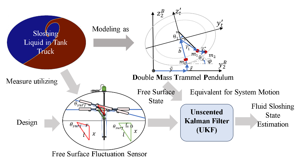
Rollover prevention of partially-filled tank trucks is an industry teaser, with the core challenge being real-time perception and observation of the liquid state inside the tank. In order realize re-liable observation of sloshing liquid, this article firstly proposes a sloshing modeling method based on multi-degree-of-freedom pendulum model, and derives the double mass trammel pendulum model (DMTP, 2DOF) accordingly, which accurately reflects the sloshing dynamics under more pervasive working conditions. Secondly, a free surface fluctuation sensor is designed based on magnetostriction, capable of measuring the inclination and height of the liquid level inside tanks filled with hazardous chemical. Finally, the unscented Kalman filter (UKF) is utilized to synthesize the information of the two, establishing a credible real-time observation of the sloshing liquid. Verified through vehicle-fluid coupled co-simulation, under condition of con-secutive double lane change, observation error of the proposed method is only 25.9% that of the open-loop calculation, providing a secure guarantee for the observation of the state variables of the single pendulum model (SP) used for most kinds of anti-rollover controller.
Keywords:
liquid sloshing
; observer
; multi-DOF pendulum model
; free surface fluctuation sensor
1. Introduction
Tank trucks, accounting for about 18% the total number of commercial trucks, play a significant role in highway transportation, whereas caused over 30% truck rollover accidents [1], attributed to their poor rollover stability caused not only by the high center of mass or heavily loaded, but also the coupling of roll movement of vehicle and sloshing liquid [2,3]. Moreover, with 80% of hazardous liquid chemicals, such as gasoline, diesel, chlorinated hydrocarbons and strong acids, etc., rely on tank trucks to be transported on highways [4], severe accidents ensue once rollover. Therefore, anti-rollover control of tank trucks is essential, and for which, the main technical approaches are to establish a more accurate surrogate model based on sloshing mechanism, designing anti-rollover control algorithms considering sloshing effect based on it, as well as measuring or estimating the required state variables for control by designing sensors and observers.
Existing models describing sloshing liquid in tanks could be generalized into 3 categories: quasi-static (QS) models, mechanical equivalent models, and fluid dynamics models.
QS models ignore the sloshing dynamics and only models the static-state position of liquid center of mass based on tank section geometric [6,7,8,9], thus have low accuracy in transient conditions.
Mechanical equivalent models approximate the force output characteristics of a liquid-filled system by establishing a mechanical model that meets the equivalence principle [10] with the original system. The commonly used models include single pendulum (SP) [11,12,13], spring-mass-damper [14], particle-cluster-rod [15], and trammel pendulum (TP) [16,17,18,19]. Most mechanical equivalent models perform well in terms of accuracy and solving speed under dynamic conditions, and can reflect the first-order sloshing, thus can be used for real-time control. However, they usually neglect higher-order sloshing such as hydraulic jump and splash, so they can only describe approximately linear sloshing well.
Fluid dynamic models, including models based on potential flow theories and finite element model based on Navier-Stokes equations (referred to as CFD method in the following text), etc., but the potential flow theory [20,21] can only be applied for certain tanks with specific section geometry under linear sloshing. Although the finite element based CFD method [22,23,24,25,26] is almost accurate under various transient conditions, it requires daunting computation thus cannot be used for real-time control.
For controller and observer design, real-time computation is essential, so the most commonly used models are various pendulum models in mechanical equivalent models, especially SP model, and whose accuracy directly affect the performance of the controller and observer.
However, the pendulum described in the model has no real world equivalent other than liquid, such the swing state of the pendulum cannot be directly measured. Therefore, it is necessary to establish an observer to estimate and update state variables of the pendulum model for controller according to the measuring of dynamics of the free surface of liquid. The collection of dynamic liquid level data is usually based on cameras [27,28,29] or ultrasonic sensors [30]. Whereas it is improper to apply transparent tanks in reality, denying measurement based on visual information. Furthermore, ultrasonic sensors need to be as perpendicular as possible to the measuring interface, making it almost impossible to be utilized for sloshing liquid.
In this article, multi-degree-of-freedom (multi-DOF) pendulum model is proposed to address the over limited range of applicable working conditions of existing mechanical equivalent models and a free surface fluctuation sensor is designed based on the magnetostriction, and a unscented Kalman filter (UKF) is applied as an observer to synthesis multi-DOF pendulum model and sensor data, which solves the problem of model phase mismatch and provides an accurate state estimation for the equivalent pendulum model (generally SP model) used for anti-rollover control of tank trucks.
2. Spectral Analysis of Sloshing Liquid
2.1. CFD modeling of Liquid Sloshing
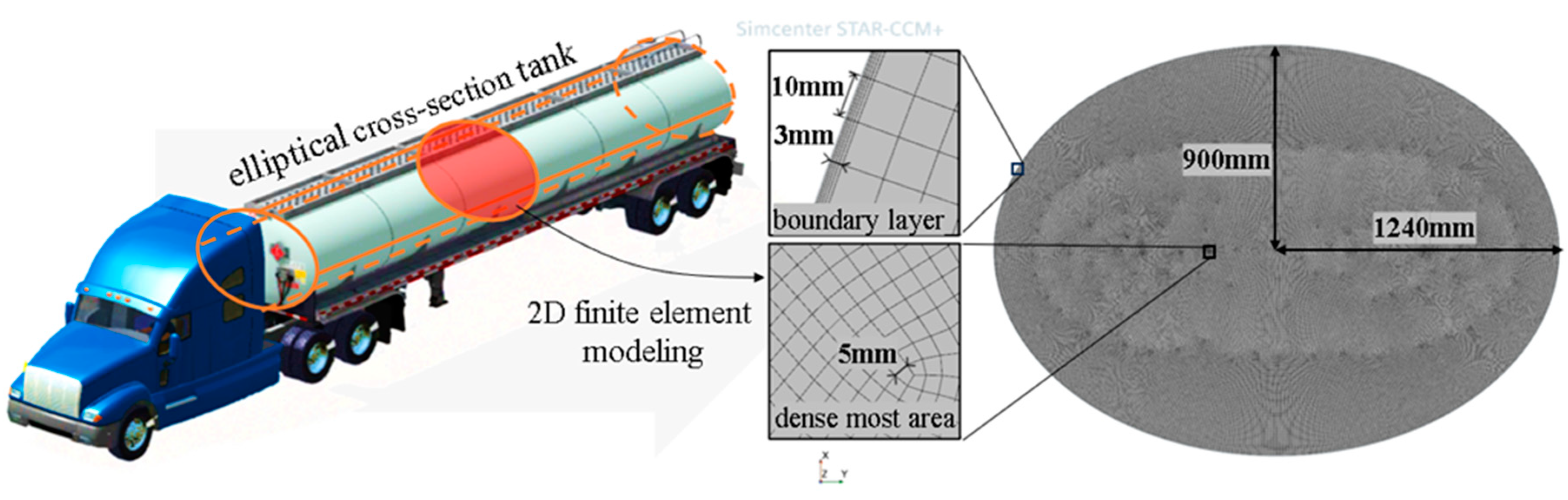
To accurately model the liquid sloshing in the tank, the accurate finite element model based CFD method is used to simulate the gas-liquid two-phase flow inside the tank. As shown in Figure 1, the research object is the lateral sloshing of an elliptical section tank of a semi-trailer tank truck, with the long axis of 1240mm and short axis of 900mm. Due to the legal regulations of installing longitudinal wave-proof plates at least at certain intervals, only the sloshing within the trailer’s roll plane is considered. In this case of neglecting longitudinal sloshing, a 2-dimensional modeling of two-phase flow is carried out by using CFD software Star-CCM+. A 3mm thick Boundary layer composed of five sub-layers of grids is set, and the maximum side length of the grid globally is controlled within 10mm, and the minimum around 5mm, which can ensure precise capture of the dynamic state of liquid sloshing in the scale of tank.
2.2. Spectral Analysis of Liquid Sloshing
According to the idea of spectral analysis, the sloshing of liquid could be decomposed into an approximate linear combination of its 0 to ∞ order sloshing mode. Illustration of sloshing modes of liquid is shown in Figure 2a, where the zero order sloshing embodies the inertia of fluid as rigid body, the 1st mode reflects the sloshing planar free surface, the 2nd move and higher order sloshing depict the sinusoidal fluctuation of free surface. The higher the order of sloshing, the less liquid participates in, but characterize more details.
Figure 1.
Elliptical cross section tank and its 2D mesh modeling in Star-CCM+.
To better understand the characteristics of the output force of sloshing liquid in the tank, CFD simulations are carried out under 3 conditions: lateral acceleration step excitation , filling rate, and the fast Fourier transform (FFT) of side-force output is performed. Lateral force output is shown in Figure 2b, the amplitude and nonlinearity of sloshing increase with a_y, and hydraulic jump and splash are also getting obvious. From Figure 2c, it can be seen that the lateral force output shows more high-frequency components with the increase of . According to Figure 2d, it is found that besides the 1st mode, the 2nd and higher order modes cannot be ignored, which explains why linear models are difficult to thoroughly describe liquid sloshing, as they ignore the higher-order sloshing components.
3. Multi-Degree-of-Freedom Pendulum Model
3.1. Generalized Pendulum Model
The most common models describing liquid sloshing are various pendulum models. Based on them, the generalized pendulum model is proposed, as shown in Figure 3, which includes simple pendulums, trammel pendulums, and all linear and/or nonlinear combinations of them. Yang et al. proposed a 1DOF multi-mass trammel pendulum to model liquid sloshing in an elliptical sectioned tank [31,32], but essentially did not increase the DOF of the pendulum, solely splitting and redistributing the concentrated swing mass, as shown in Figure 3c, and has no substantial difference in terms of swing mode with trammel pendulum with 1 swing mass. Different pendulum models differ in the number of swinging DOF and the number of concentrated masses, which gives them diverse potential in describing liquid sloshing. Theoretically, the higher the DOF is, the stronger its fitting ability, but also more prone to overfitting and require more computation. Therefore, it is important to choose a suitable generalized pendulum model to balance computational complexity and accuracy.
3.2. Spectral Analysis of Models
Spectral analysis was conducted on different sloshing models, with results shown in Table 1. The rigid body model can only embody the inertia of the rigid body (zero order sloshing), whereas QS model can express the inertia together with free surface inclination angle (and the movement of the liquid center of gravity caused by it), but cannot express the sloshing dynamic. A linearized SP model can only express up to 1st mode; SP and TP can express 2nd and 3rd mode, but their accuracy is low for higher-order sloshing. Multi-DOF Pendulum can express high-order sloshing, but its accuracy is not as accurate as that of the finite volume method based CFD model (FVM-CFD), but the latter is too clumsy to compute in Real-time. Therefore, in order to obtain a more accurate model while balancing computational complexity, the DOF of the pendulum model can be appropriately increased.
3.3. 2DOF Pendulum Models
On the basis of existing models SP and TP, dual mass trammel pendulum (DMTP) and combined trammel and single pendulum (TPSP) models with 2DOF are proposed, which are nonlinear and linear combinations (series and parallel) of SP and TP, respectively. According to Lagrange equation, their dynamic model can be deduced.
To realize the input of lateral, vertical acceleration, and roll angular acceleration of the trailer to the model, 3 additional DOFs besides those 2 of DMTP should be considered, which are the lateral, and vertical translational DOF, , and rotational DOF around axis. The derivation of the dynamic equation using the Lagrange method is shown as follow.
Generalized coordinates: , degree of freedom: 5 (2 swinging DOFs are of DMTP, 3 additional are essentially that of trailer), and only 2 differential equations of is needed since DMTP has 2 DOFs.
According to Lagrange equation
where is the kinetic energy of system, is the potential energy of the system, is the corresponding generalized force of the th DOF, the kinetic and potential energy expression and of the 2DOF system consisting concentrated masses , , and are needed.
Vectorized expression of concentrated masses position are as (2), (3), and (4).
Derive position vectors in (2), (3), and (4) to obtain velocity vectors in (5) and acceleration vectors in (6).
where is velocity component of the th mass along positive direction of axis ,the same expression is true for acceleration component .
The kinetic energy of system is as in (7),
where is the th concentrated mass.
When taking as the reference potential energy surface, potential energy of the system is as in (8),
where is the gravitational acceleration.
Lagrangian of the system is defined as (9).
Differential equation results could be obtained according to (7), and exact expressions can be acquired through the build in function of MATLAB:. Rearrange results to get the Second-order differential equations of as in (10) and (11).
Noted that a damping term is added after (10) and (11) to mimic damping effect of liquid system, where and are constant damping coefficients.
Numerical integration is used to solve the dynamic process of DMTP, where the inputs of the 2 equations (10) and (11) are from trailer, other variables are taken as state variables of the system. The solution of 3 generalized forces (namely lateral force , vertical force , and roll moment ) is as follows.
In (12), (13), and (14), the negative sign represents the reversion of force direction, representing the force exerted by the liquid on the tank. The derivation of TPSP model shown in Figure 4c,d is the same with DMTP, which need just slight modifications to the expression of in (2), (3), and (4) accordingly.
4. Simulation Analysis of Pendulum Models
4.1. Parameter fitting for pendulum models
To obtain the parameters of the pendulum model and compare SP, TP, as well as the proposed DMTP and TPSP models, a lateral acceleration step excitation CFD simulation dataset: dataset NO.1, as shown in Figure 5., was established, which includes 30 sets of simulation data, reflecting the free sloshing of liquid. Secondly, the loss function representing model fitness is defined in (15).
where ,, and are time average value of , , and . , , and are the lateral force, vertical force, and roll moment output of model under step excitation of .
Genetic algorithm is applied to optimize the loss function so as to fit the optimal structural parameters of the model. To ensure convergence, each model is recalculated 8 times at each filling rate, and the optimal result is taken as the fitting parameter. The optimization results are shown in Figure 6. SP is better than TP at medium to high filling rates, whereas DMTP is the optimal model under all examined filling rates, followed by TPSP, reflecting the higher fitting potential of the two proposed 2DOF models compared to conventional 1DOF models.
4.2. Map Analysis of Pendulum Models
To verify the generalization ability of models in other working conditions, firstly, another CFD simulation dataset: dataset No.2 with 150 sets of data is established, as shown in Figure 7, with lateral acceleration sinusoidal excitation, to reflect the forced sloshing of liquid.
On top of that, the orthogonal conditions of sinusoidal excitation with different amplitude and frequency are verified on datasets NO.1 and NO.2, and the normalized errors of force outputs , , and of the 4 pendulum models calculated using the optimal fitting parameters are compared with the CFD results. Errors are shown in Figure 8. The larger and darker the blue area, the better the model conforms to more working conditions. DMTP is the optimal model at medium to low filling rates , whereas at higher filling rates, sloshing effect attenuates, and all models achieve almost the same performance, and therefore, the optimal model in this case is SP which requires the least computation. To some extent, the advantages of DMTP as a more accurate pendulum model have been verified.
DMTP is a nonlinear pendulum model with more computation than traditional 1DOF models, but can still be real-time computed even on STM platform for general use with main frequency of only 24MHz. Although limited by the high operation frequency of model predictive controllers, it would be difficult to use DMTP as a predictive model in MPC controllers, but it is proper to use it as the system motion equations in the observer with a lower frequency (about 1000 times of simulation per second and below) to improve observation accuracy.
5. Sloshing Observer Design
5.1. Free Surface Fluctuation Sensor Design
As mentioned in section I, considering computational burden, existing research typically use linearized SP within the controller to describe liquid sloshing so as to exert anti-rollover control. However, linear models are not precise enough thus requires external measurements or estimates to unremittingly update model states. As shown in Figure 9a, state variables of the vehicle model are all available through direct/indirect measurement of existing sensors, or estimated, like lateral velocity (or sideslip angle , ) [33,34,35]. Nevertheless, state variables related to liquid (pendulum) models, such as swing angle and angular velocity , can neither be obtained through existing sensor, nor by estimation from available vehicle states, since information of liquid in vehicle states is limited, and therefore, theoretically, an unrealistic extremely accurate vehicle model is needed to estimate liquid state.
Existing works invoking pendulum model assumption to control vehicles do not involve real vehicle tests, with only simulations in which pendulum substitute liquid were carried out [12,13,18,19], and state variables (e.g., swing angle ) are directly fed back to the controller for state update, ignoring the fact that instead of a pendulum, there exists only liquid in actual tank, which is currently unable to be measured.
Error characteristics of open-loop calculation of models is shown in Figure 9b. Due to the fact that, frequency of system response tends to be consistent with that of excitation, accumulation of phase difference is relatively slow during forced sloshing (stage 1) starting from the calm state (stage 0). When a maneuvering (steering, lane changing, etc.) is complete and start to drive stably, free sloshing begins (stage 2), and the slight discrepancy between the actual sloshing frequency and the model’s natural frequency is amplified, and phase difference accumulates swiftly. On the other hand, due to the damping caused by internal friction of liquid, i.e., the unobservable mode is asymptoticly stable, the system is detectable, thus after a period of time, the phase difference is effaced (stage 3) and system restores calm (stage0). But if maneuver again on stage 2 or stage 3, it causes the accumulation of phase error, and when accumulated to a certain extent, model mismatch happens leading to controller failure and eventually rollover. Therefore, a free surface fluctuation sensor is designed to measure the liquid state so as to estimate states of a pendulum model.
As shown in Figure 10, a magnetostrictive liquid level meter constitutes the main part of the fluctuation sensor. Floating balls containing permanent magnet slide on measuring rod and the level meter functions through timing the round-trip of torsional stress wave from the digital head to the magnets in balls.
Existing level meter capable of simultaneous measurement of positions of multiple floating balls reach accuracy of 0.5%/0.3mm (larger one), and the maximum measurement frequency reaches 2500-4000Hz.
Based on the level meter, a rocker arm as well as a retractable floating board are complemented to form a measurement triangle as shown in Figure 10b. Parameters of the measuring triangle are selected in advance, and the distance between the upper and lower floating balls differs with liquid free surface inclination angle. Through Law of cosines in (16),
the inclination angle fitted by the floating board can be obtained, where is the average inclination of the liquid surface measured by the sensor, is the center distance between upper floating ball and the hinge on one side of the central float board, is the distance between the upper and lower floating balls measured by the sensor, and is the designed length of the rocker arm.
Common range of surface inclination is generalized by analyzing simulation results, it is found that under large acceleration step excitation (), the liquid level inclination does not exceed , and in reality, such a large lateral acceleration is scarce. For safety consideration, is chosen as the measurement range. Due to regulatory limitations [2,3], the maximum filling rate must not exceed 95%, and since the impact of liquid sloshing at high filling rates can even be ignored, therefore, in order to ensure the measurement range of at the highest design filling rate and cover at least 1/2 of the free surface width at the lowest design filling rate to filter out the impact of 3rd mode and higher order sloshing, the geometric parameters of the floating board are designed as shown in Figure 10c.
As in Figure 10d, by using a lightweight pulley block with a specific magnification, the floating board length can be automatically adjusted according to the filling rate under the balance of the buoyancy of floating board and the elastic restoring force of the recovery spring.
Under general sloshing conditions that do not cause severe breakage of the liquid surface, swing angle of SP in controller can be approximated as the linear transform of , i.e.,
where is a constant.
5.2. Observer Based on DMTP and Senser Data
According to the accurate nonlinear model DMTP and the data of the fluctuation sensor, an observer based on unscented Kalman filter (UKF) can be designed to estimate the swing angle of the linearized SP required in the controller, as shown in Figure 11.
5.2.1. Fusion of angles of DMTP to Linearized SP
From Section 4, it can be seen that the open-loop accuracy of DMTP is optimal at medium filling rates and below (), but linearized SP in the controller has with only 1 DOF i.e., Similarly, the fluctuation sensor can only measure the average inclination angle , so how to equal the angle of 2 DOFs of DMTP i.e., , to is an urgent problem.
There are two methods fusing 2 angles, as shown in Figure 12b,c.
* CG method in legend correspond to (18-19), conv1 method to (21), conv2 method to (22).
Center of Mass conversion method: takes the angle of C.G. of and in DMTP as , i.e., (18), (19),
Convex combination method: assume as the convex combination of and , i.e., (20),
where the combination proportion is determined by relationship between and , as in (21)
or in (22).
Through simulation of the 2 methods above in extreme maneuvering conditions, i.e., left cornering, (high speed) single lane change, and (short distance) double lane change, on the vehicle-fluid coupling co-simulation platform which is to be constructed in section VI, A, the equivalent fusion angle is obtained and then be input into force output calculating equations for SP. Results is shown in Figure 12d–f.
It can be concluded that the convex combination method with (20) and (22) is the most apropos one, since the time average error of force outputs (, , and ) of the whole simulation process being the lowest (correspond to the final value of the last inset of Figure 12d–f), and the fusion results is superior to that of the open-loop calculation of SP.
5.2.2. Decomposition of angle from Linearized SP to DMTP
Except for the fusion method, the construction of system equations of motion (23) for UKF
where symbolizes discrete time, is the swing angle of linearized SP, is the system input, , is the process noise, requires the decomposition of to and (in this article, a check above variables implies prior, and a hat implies posterior) if DMTP is to be engaged. But the direct conversion of low dimensional data to a higher on is impossible due to the conversion exists null space, thus which being calculated at time step are needed to support the estimation. The decomposition of to and can be seen as an optimization problem: find closest to , while subject to the relationship found in (20), i.e., , the problem can be described as (24).
Let , , the constrain is converted to (25).
After substituting the constraint conditions, the cost function is
let the partial of to be 0
the optimal solution is
Construct decomposition function (29) according to (28).
Construct angle fusion function (30) according to (20) and (22).
The partial differential function of DMTP can be generalized as (31).
where contains the state variables of DMTP , and equation of system motion is as (32).
Since the Equations of system motion involves DMTP, which is difficult to linearize, and UKF does not even need the analytical form of the motion and observation equations simply regard the system as a black box, so UKF is applied for observer construction.
5.2.3. Construction of UKF
Firstly, the prediction part: write the state and motion noise together in a joint form, assume their dimension as , and define a new variable,
and
where is the mean of , is the covariance matrix of , is the covariance of posterior in time step , and is the covariance of process noise in time step .
Step1, substitute the unscented transformation of in equations of system motion in (32).
Perform the Cholesky decomposition of
where is a lower triangular matrix
in which
and substitute and into (32).
The mean of predicted prior is and its covariance is
where the coefficient is
Step 2, to correct prediction with observation
Likewise, is defined as the joint form of prediction mean and the observation noise
and
where is the covariance of observation noise . Unscented transformation is also performed as in (35), and (35), where
Substituting and into observation function
Posterior is constructed and mean of observation , covariance of observation , and covariance of and are obtained.
The Kalman gain is defined in (49)
Posterior mean is
whose covariance is
UKF cannot guarantee convergence in general nonlinear systems, but its iterative version of the Iterated Unscented Kalman filter (IUKF) can theoretically converge to the posterior mean of the true value. However, due to the assumption that the observation equation is linear as (17), IUKF is equivalent to UKF. In theory, UKF converge to the posterior mean of the equivalent pendulum angle of linearized SP.
In practical applications, it is found that there exists some local fluctuations in the sensor data difficult to be filtered out, which will cause impact when calculating the force output. Therefore, a Luenberger observer is added after the sensor data to smooth the it, and its two poles are designed as [−5, −5].
6. Simulation and Analysis of Sloshing Observation
6.1. Simulation model
To better validate the effectiveness of the observer constructed in last section, a vehicle-fluid coupling co-simulation verification platform is built as shown in Figure 13.
By writing MATLAB Function and Java Macro, Simulink and StarCCM+ are controlled to read and write data automatically in the simulation process, and two flag bit sharing files and two data exchange sharing files are constructed to realize the co-simulation of Vehicle dynamics and finite element based CFD. With the help of this simulation platform, real-time interaction between vehicles and fluid dynamics can be more realistically simulated.
A simulation model is built in Simulink as shown in Figure 14, to validate the proposed observing method based on multi-DOF pendulum model (specifically DMTP model) and the free surface fluctuation sensor.
6.2. Acquisition of fluctuation sensor data
As currently no physical prototype of fluctuation sensor is available, simulation methods are used to simulate it. As shown in Figure 15, sensor data is obtained through image processing using CFD simulation images output by Star-CCM+. The specific method is:
Step 1: At each simulation moment, Star-CCM+ outputs an image of liquid shaking.
Step 2 grayscale the image and extract edges.
Step 3 masks the parts of the image irrelevant to the free liquid level, and trim the free surface according to the length of the floating board.
Step 4 Obtaining equivalent sensor data .by fitting scatter points of the trimmed liquid surface with a straight line.
6.3. Results analysis
As analyzed in Figure 9b, error of open-loop calculation of the model accumulates swiftly under continuous maneuvering conditions, making it the most effective condition to test the performance of the proposed observing method. Therefore, the consecutive double lane change condition is designed as shown in Figure 16a, reference path is two double lane change paths with an interval of only 100m. Each double lane change path completes lane change within 45m, with a 45m straight line and change back within another 45m. The initial speed of semi-trailer tank truck is 70km/h.
The simulation results are shown in Figure 16b–g, using the lateral acceleration a of the trailer and roll angular velocity from TruckSim (In real vehicles, they can be measured by the IMU fixed at the bottom of the liquid tank) Add white noise to and with a variance of 0.001 to reflect the measured noise of IMU as the input of the UKF’s equations of system motion, and fluctuation sensor measured result is supplemented for state estimation.
Figure 16e compares the angle fusion results with the angle calculated by open-loop SP and DMTP, and Figure 16f compares the roll moment obtained by inputting the fusion results and the equivalent angle calculated by open-loop SP into the force calculation formula of SP, and the roll moment output by CFD. Figure 16g compares the time average error of the predicted roll moment whether through the proposed observation method (data fusion method) or the open-loop method with CFD results (the error at each moment is the average of all previous moments’ errors, and the value at the last moment represents the mean error during the entire simulation process). Before the 10th seconds, the open-loop model has enough accuracy, whereas as the first double lane change ends, the liquid in tank enters the free sloshing state. At this point, the tiny difference between the model’s natural frequency and that of the actual liquid-filled system begin to manifest, and phase difference accumulates. Before the damping effect of the system could eliminate the accumulated errors, the vehicle begins the second double lane change, which caused the quick accumulation of the errors of the open-loop calculation. However, the proposed observation method that introduces fluctuation sensor data consistently maintained high measurement accuracy. The time mean observation error (9104Nm) during the whole process is only 25.9% the time average error (35177Nm) of open-loop calculation, which improved the observation accuracy significantly by about 4 times. And especially during the second maneuvering, the instantaneous error is only round 1/7 that of the open-loop observation.
7. Conclusion
In order to realize reliable observation of states of the pendulum model (reflecting liquid sloshing dynamics) for anti-rollover control of tank trucks, to begin with, this article proposes a modeling method for liquid sloshing in the tank of tank trucks based on a multi-degree-of-freedom (multi-DOF) pendulum model by conducting spectral analysis of the output force characteristics of liquid sloshing in the tank, and designed the double mass trammel pendulum model (DMTP, 2DOF) and the combined trammel and single pendulum model (TPSP, 2DOF) that reflect the sloshing dynamics more accurately especially under medium and low filling rates (). Through simulations under orthogonal working conditions of step and sinusoidal lateral acceleration excitation, DMTP and TPSP are proved to have advantages over conventional 1 degree-of-freedom pendulum models (i.e., SP and TP) in terms of generalization ability and precision.
In addition, a free surface fluctuation sensor is designed which can measure the inclination and average height of the sloshing liquid surface. It includes a retractable floating board that can automatically adjust its length according to changes in filling rate. The characteristic that the measurement part has no electronic components makes it suitable for applications in tanks containing hazardous fluid chemicals. Furthermore, unscented Kalman filter (UKF) is applied to observe the liquid sloshing.
In the end, through the constructed vehicle-fluid coupling co-simulation verification platform, the simulation in working condition of consecutive double lane change is carried out in the way of tight coupling between vehicular dynamics and CFD, which verifies the feasibility of the proposed observation method based on the multi-DOF pendulum model and free surface fluctuation sensor, and its advantages over the conventional open-loop calculation method, providing reliable observation for the state observation of the for controllers, ensuring the safety of practical application of control algorithms under extremities.
Due to the limitations of the simulation model, this article only discusses the situation of liquid sloshing in the roll plane, neglecting the longitudinal flow of liquid in the tank and the impact of longitudinal flow on lateral sloshing under conditions including obvious acceleration and/or braking. In the future, the coupling of lateral and longitudinal sloshing will be considered in modeling, and the fluctuation sensor would be prototyped. The model car tests would be carried out with the integrated control algorithm of rollover prevention and trajectory tracking based on model predictive control.
Author Contributions
Conceptualization, X.Q. and B.G.; methodology, X.Q.; software, X.Q.; validation, X.Q., Y.Z.; formal analysis, X.Q.; investigation, X.Q; resources, Y.Z.; data curation, X.Q.; writing—original draft preparation, X.Q.; writing—review and editing, B.G. and Y.Z.; visualization, X.Q.; supervision, B.G. and Y.Z.; project administration, B.G.; funding acquisition, B.G. All authors have read and agreed to the published version of the manuscript.
Funding
This research was funded by the National Key Research and Development Program of China, grant number 2021YFB2501000, and funded by Tsintel Automotive Technology (Suzhou) Co. Ltd.
Institutional Review Board Statement
Not applicable.
Informed Consent Statement
Not applicable.
Data Availability Statement
Not applicable.
Acknowledgments
We gratefully acknowledge the support from the above fund and cooperation.
Conflicts of Interest
The authors declare no conflict of interest.
References
- Transportation Committee of China Railway Enterprise Management Association, Transport of Dangerous Goods by Railway Tank Vehicles, 1st ed., China: China Railway Publishing House, 2014, pp. 71-72.
- Road Transport of Liquid Dangerous Goods Tank Vehicles Part 1: Technical Requirements for Metal Atmospheric Tank Bodies, GB18564, 1-2006.
- Supervision Regulations for Safety Technology of Mobile Pressure Vessels, TSG R0005-2011, 5-2011.
- WU Zong-zhi, and SUN Meng, “Statistic analysis and countermeasure study on 200 road transportation accidents of dangerous chemicals,” Journal of Safety Science and Technology, Apr. 2006, vol. 2, no. 2, pp:3-8. [CrossRef]
- JIA Xinhong, ZHANG Zhulin, and JIANG Defei, “Research Status of Influence of Liquid Sloshing in Tank on Rollover Stability of Semi-loaded Tank Truck,” Automobile Applied Technology, Jan. 2022, vol. 47, no. 1, pp:193-196.
- HUANG Yang, DENG Gui-de, and ZHANG Xing-fang, “Analysis of Instant Liquid Shock Effect of Non-Full-Filled Tank in Course of Turning,” Chemical Machinery, 2017, vol. 44, no. 5, pp:558-563.
- CHEN Yi-bao, RAKHEJA Subhash, and SHANGGUAN Wen-bin, “Modified design and safety analysis of tank cross section based on roll stability,” Journal of Vibration and Shock, Jun. 2016, vol. 35, no. 6, pp:146-151.
- WANG Xiaorun, CHEN Qinghua, and WANG Jianye, “Analysis on the Influence of Lateral Acceleration on Lateral Stability of Non-Full-Load Liquid Tanker,” Journal of Anhui Polytechnic University, Aug. 2022, vol. 37, no. 4, pp:10-24.
- HE Lieyun, and LIU Qiang, “A Quasi-static Equivalent Mechanical Model for Roll Stability of Partially-filled Tanker Trucks,” Mechanics in Engineering, Jun. 2020, vol. 42, no. 3, pp:294-299. [CrossRef]
- WANG Zhaolin, and LIU Yanzhu, Dynamics of Liquid-Filled Systems, 1st ed., China: Science Press, 2002.
- XU Xiaomei, ZHU Chengwei, and CAI Haohao, “Study on the driving stability of lane change for semi-trailer liquid tanker based on simulation platform,” Experimental Technology and Management, Aug. 2022, vol. 39, no. 8, pp:96-100.
- Zhao Weiqiang, Ling Jinpeng, and Zong Changfu, “Development of Anti-rollover Control Strategy for Liquid Tank Semi-trailer,” Automotive Engineering, 2019, vol. 41, no. 1, pp:50-56. [CrossRef]
- ZHAO Wei-qiang, FENG Ran, and ZONG Chang-fu, “Anti-rollover control strategy of tank trucks based on equivalent sloshing model,” Journal of Jilin University (Engineering and Technology Edition), Jan. 2018, vol. 48, no. 1, pp:30-35. [CrossRef]
- YU Di, LI Xian-sheng, LIU Hong-fei, ZHENG Xue-lian, and XU Yi, “Research on Roll Stability Model of Partially-filled Tankers,” Journal of Hunan University (Natural Sciences), Aug. 2016, vol. 43, no. 8, pp:40-44. [CrossRef]
- Gonzalo Guillermo Moreno Contreras, et al., “Stability of tanker trucks using the Davies method,” Journal of Applied Engineering Science, 2022,vol. 20, pp: 602-609. [CrossRef]
- Di Yu, and Jiangwei Chu, “.Study on roll-stability model optimization for partially filled tanker trucks,”. Advances in Mechanical Engineering (Sage Publications Inc.), 2019, vol. 11, pp: 1-8. [CrossRef]
- Salem, and Mohamed Ibrahim, “Rollover stability of partially filled heavy-duty elliptical tankers using trammel pendulums to simulate fluid sloshing,” Ph.D. dissertation, West Virginia University, 2000.
- REN Yuanyuan, Li Xiansheng, ZHENG Xuelian, and WANG Jie, “Accurate Dynamics Modeling and Roll Stability of Tank Vehicle,” Journal of Shanghai Jiao Tong University, Mar. 2020, vol. 54, no.3, pp:312-321. [CrossRef]
- WAN Ying, “Study on Vehicle-Liquid Coupling Dynamic Characteristics and Anti-Rollover Control Method for Tank Vehicles,” Ph.D. dissertation, Dept. College Auto. Eng., Jilin Univ., Changchun, China, 2018.
- YU Zhixin, CHENG Xinxin, LI Jie, and LI Shaosong, “Simulation analysis of lateral stability for liquid tank truck based on model predictive control (MPC),” Journal of Changchun University of Technology, Jun. 2018, vol. 39, no. 3, pp:224-232.
- YU Zhixin, LI Jie, CHENG Xinxin, DAI Fuguang, and LI Shaosong, “Simulation on the optimal control of the stability of liquid tank truck,” Oil & Gas Storage and Transportation, Aug. 2019, vol. 38, no. 8, pp:885-891.
- Matthew Aquaro, Victor H. Mucino, Mridul Gautam, and Mohammed Salem, “A Finite Element Modeling Approach for Stability Analysis of Partially Filled Tanker Trucks,”.SAE Transactions, 1999, vol.108, pp: 452-460. [CrossRef]
- MAO Haijian, LI Bo, BEI Shaoyi, DING Yue, and QUAN Zhengqiang, “Research on Roll Stability of Liquid Tanker Based on Fluid-solid Coupling,” Journal of Jiangsu University of Technology, Aug. 2021, vol. 27, no. 4, pp:56-67.
- LI Jie, YU Zhixin, CHENG Xinxin, DAI Fuguang, and LI Shaosong, “Simulation of stability control of tank trucks under vehicle-liquid coupling response,” Oil & Gas Storage and Transportation, Feb. 2020, vol. 39, no. 2, pp:188-194.
- Liu Kui, and Kang Ning, “Simulation of liquid sloshing in braking process of tank truck,” Journal of Beijing University of Aeronautics and Astronautics, Jul. 2009, vol. 35, no. 7, pp:799-803.
- Liu Kui, and Kang Ning, “Simulation of liquid sloshing in turing process of tank truck,” Journal of Beijing University of Aeronautics and Astronautics, Nov. 2009, vol. 35, no. 11, pp:1403-1407.
- Guagliumi L, Berti A, Monti E, et al., “A Simple Model-Based Method for Sloshing Estimation in Liquid Transfer in Automatic Machines,” IEEE Access, Sep. 2021, vol. 9. pp: 129347-129357. [CrossRef]
- Roberto Di Leva, Marco Carricato, Hubert Gattringer, and Andreas Müller, “Sloshing dynamics estimation for liquid-filled containers performing 3-dimensional motions: modeling and experimental validation,” Multibody System Dynamics, 2022, vol. 56, pp: 153-171. [CrossRef]
- Tosun Ufuk, Aghazadeh Reza, Sert Cüneyt, and Özer Mehmet Bülent, “Tracking free surface and estimating sloshing force using image processing,” Experimental Thermal and Fluid Science, 2017, vol. 88, pp: 423-433. [CrossRef]
- S M Nashit Arshad, Yasar Ayaz, Sara Ali, A.R. Ansari, and Raheel Nawaz, “Experimental Study on Slosh Dynamics Estimation in a Partially Filled Liquid Container Using a Low-Cost Measurement System,” IEEE Sensors Journal, 2022, vol.22, no.16, pp: 16212-16222. [CrossRef]
- YANG Xiu-jian, XING Yun-xiang, WU Xiang-ji, and ZHANG Kun, “Multi-mass trammel pendulum model of fluid lateral sloshing for tank vehicle,” Journal of Traffic and Transportation Engineering. Oct. 2018, vol. 18, no. 5, pp: 140-151.
- Wu Xiangji, Yang Xiujian, and Song Juntao, “Study on Liquid Lateral Sloshing Model of Tank Vehicle,” Agricultural Equipment & Vehicle Engineering, Feb. 2018, vol. 56, no. 2, pp:7-15.
- Zhang Buyang, Zong Changfu, Wang Huaji, and Zheng Hongyu, “State Estimation of Heavy Tractor Semitrailers Based on Adaptive Kalman Filter,” Automobile Technology, 2012, vol. 1, no. 7, pp:1-5.
- Yu Zhixin, “Research on Dynamics Stability Multi-objective Control Based on Model Predictive Control for Heavy Duty Semi-trailer,” Ph.D. dissertation, Dept. College Auto. Eng., Jilin Univ., Changchun, China, 2015.
- Feng Ran, “Research on Key Parameters Estimation and Anti-rollover Control of Liquid-filled Tractor-Semitrailer,” M.S. thesis, Dept. College Auto. Eng., Jilin Univ., Changchun, China, 2018.
Figure 2.
(a) Different sloshing mode of liquid in tank; (b) CFD simulation under step excitation ; (c) Lateral forces from liquid to tank; (d) FFT transformation of side forces.
Figure 2.
(a) Different sloshing mode of liquid in tank; (b) CFD simulation under step excitation ; (c) Lateral forces from liquid to tank; (d) FFT transformation of side forces.
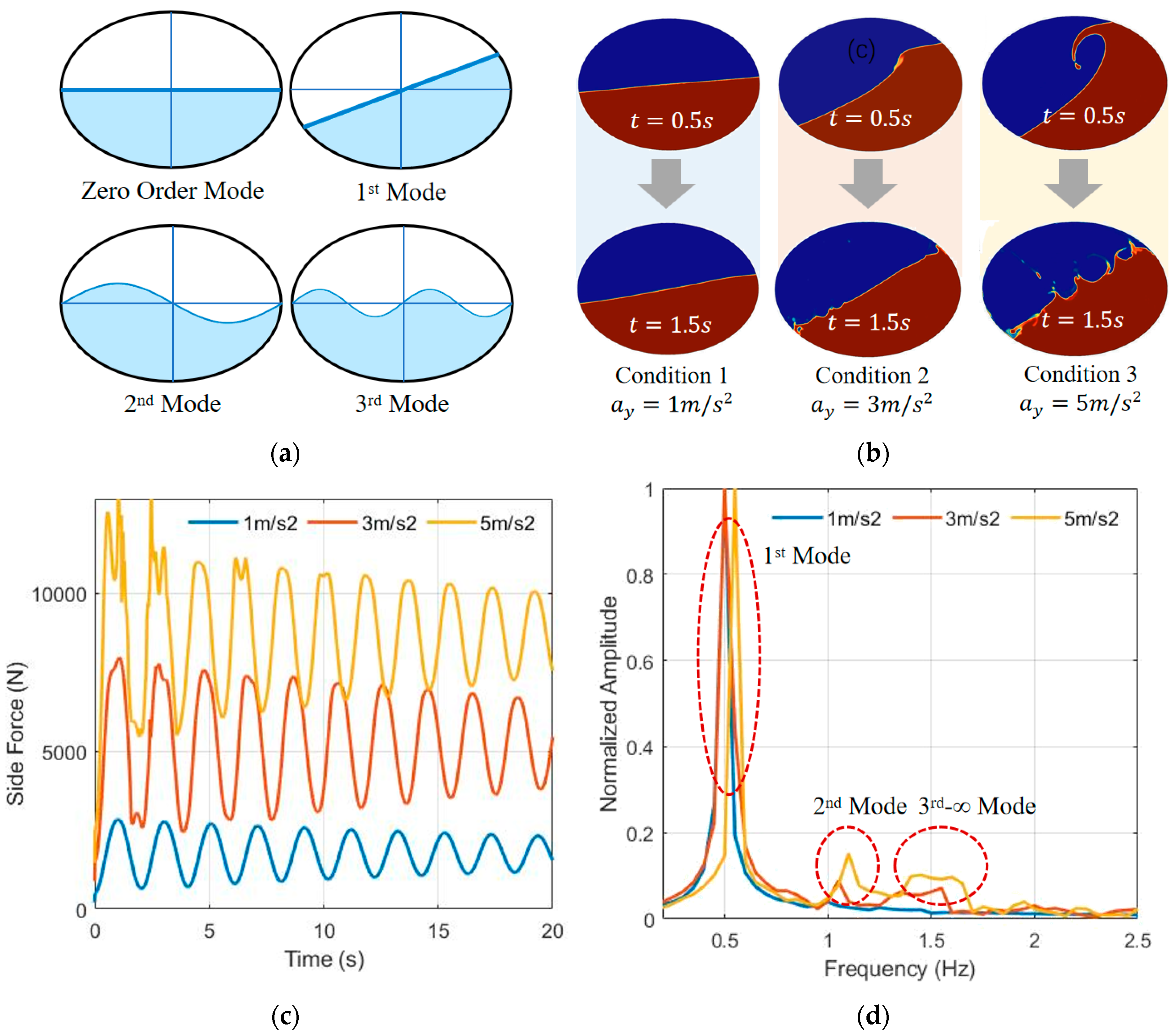
Figure 3.
Examples of general Pendulum models. (a) Single pendulum, 1DOF, 2 concentrated-masses (1 swinging, 1 fixed); (b) Trammel pendulum, 1DOF, 2 concentrated-masses (1 swinging, 1 fixed); (c) 1DOF multi masses trammel pendulum [31,32]. 1DOF, n+1 concentrated-masses (n swinging, 1 fixed); (d) Multi-DOF trammel pendulum, n DOF, n+1 concentrated-masses (n swinging, 1 fixed); (e) Linear combination of SPs and TPs, n DOF, n+1 concentrated-masses (n swinging, 1 fixed); (f) Non-linear combination of SPs and TPs, n DOF, n+1 concentrated-masses (n swinging, 1 fixed)..
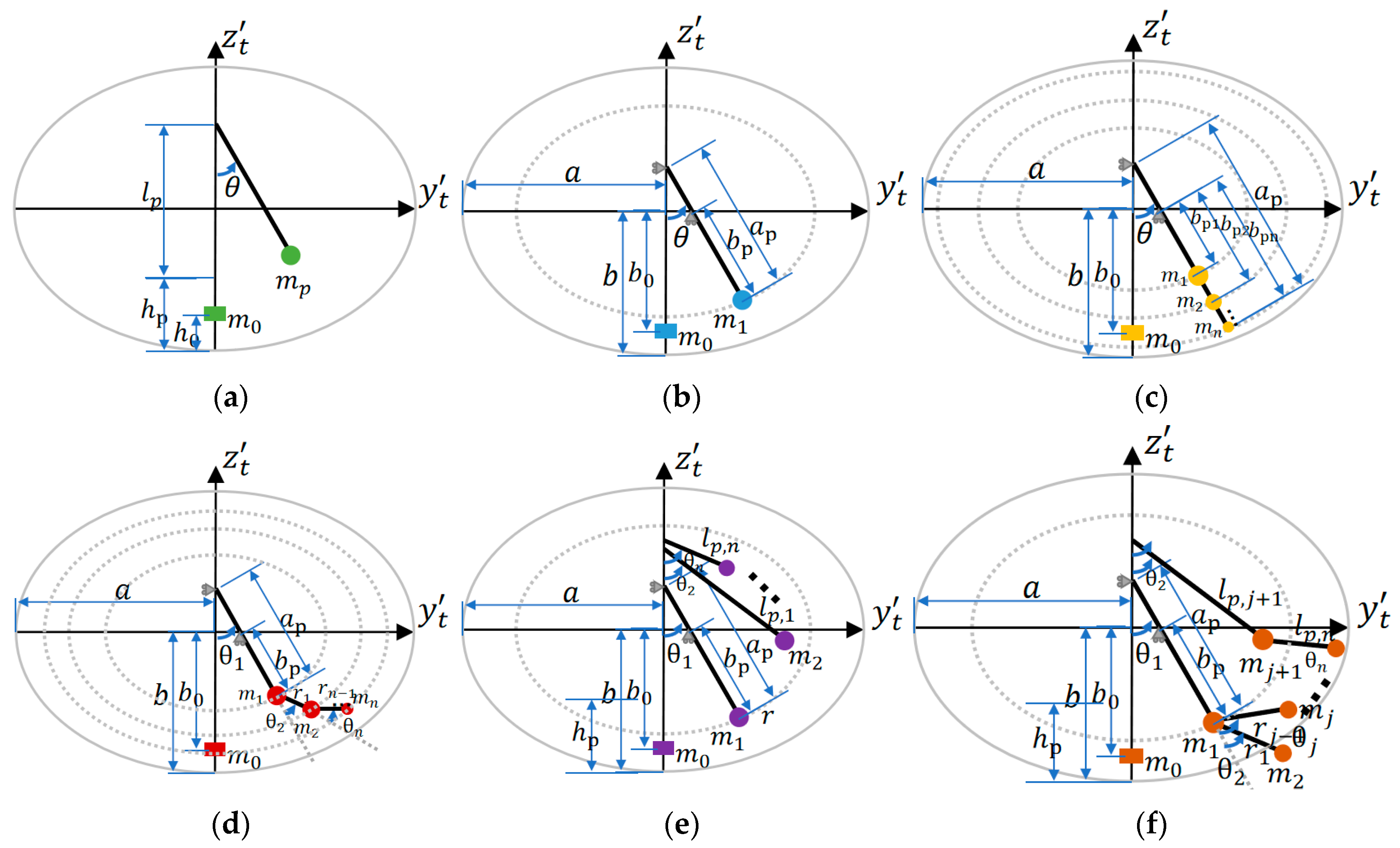
Figure 4.
Proposed 2-DOF pendulum model DMTP and TPSP, where is the coordinate fixed on trailer body, and is the coordinate fixed on tank with located on the center of elliptical center. (a) Geometry parameters of DMTP; (b) Degree of freedom and dynamics of DMTP; (c) Geometry parameters of DMTP; (d) Degree of freedom and dynamics of DMTP.
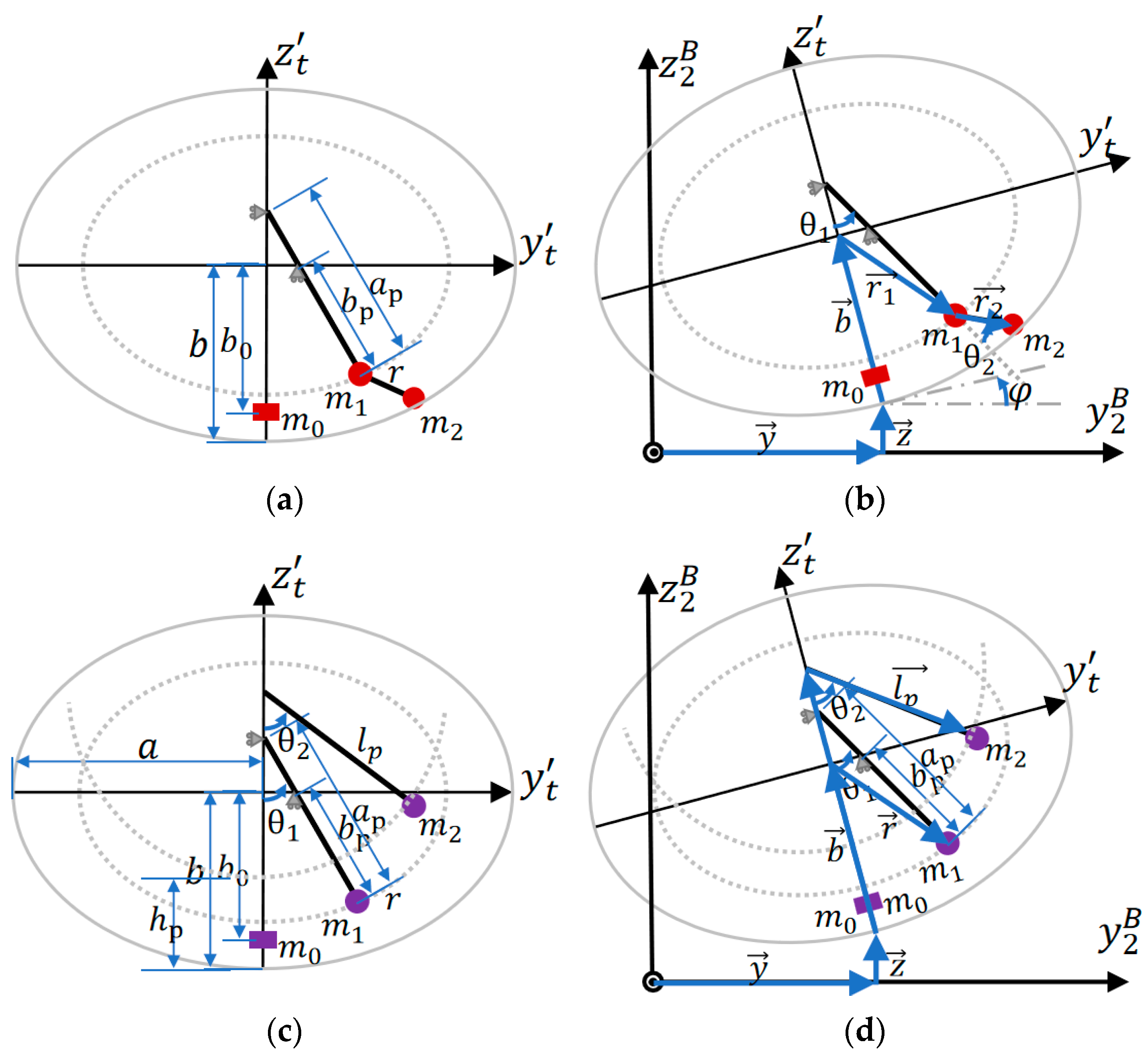
Figure 5.
CFD simulation dataset No.1: with step excitation of lateral acceleration, , (a–f) , respectively.
Figure 5.
CFD simulation dataset No.1: with step excitation of lateral acceleration, , (a–f) , respectively.
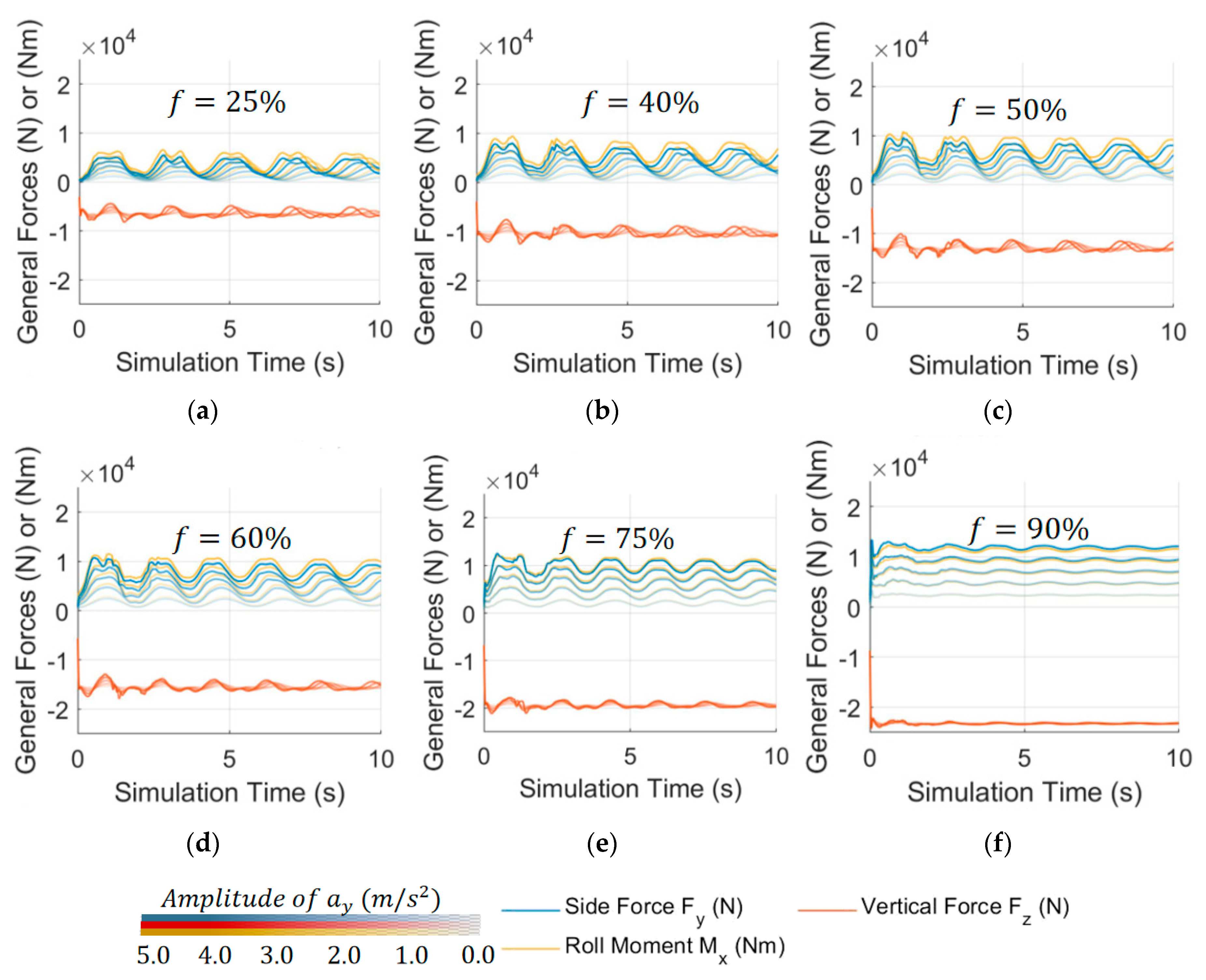
Figure 6.
Cost function optimization results, solid lines indicate the best result in 8 trials, shading indicates results distribution.
Figure 6.
Cost function optimization results, solid lines indicate the best result in 8 trials, shading indicates results distribution.
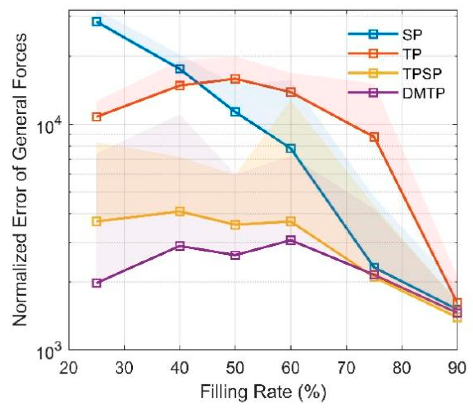
Figure 7.
CFD simulation dataset No.2: with sinusoidal excitation of lateral acceleration, , (a–e) , respectively.. 150 CFD simulations totally.
Figure 7.
CFD simulation dataset No.2: with sinusoidal excitation of lateral acceleration, , (a–e) , respectively.. 150 CFD simulations totally.
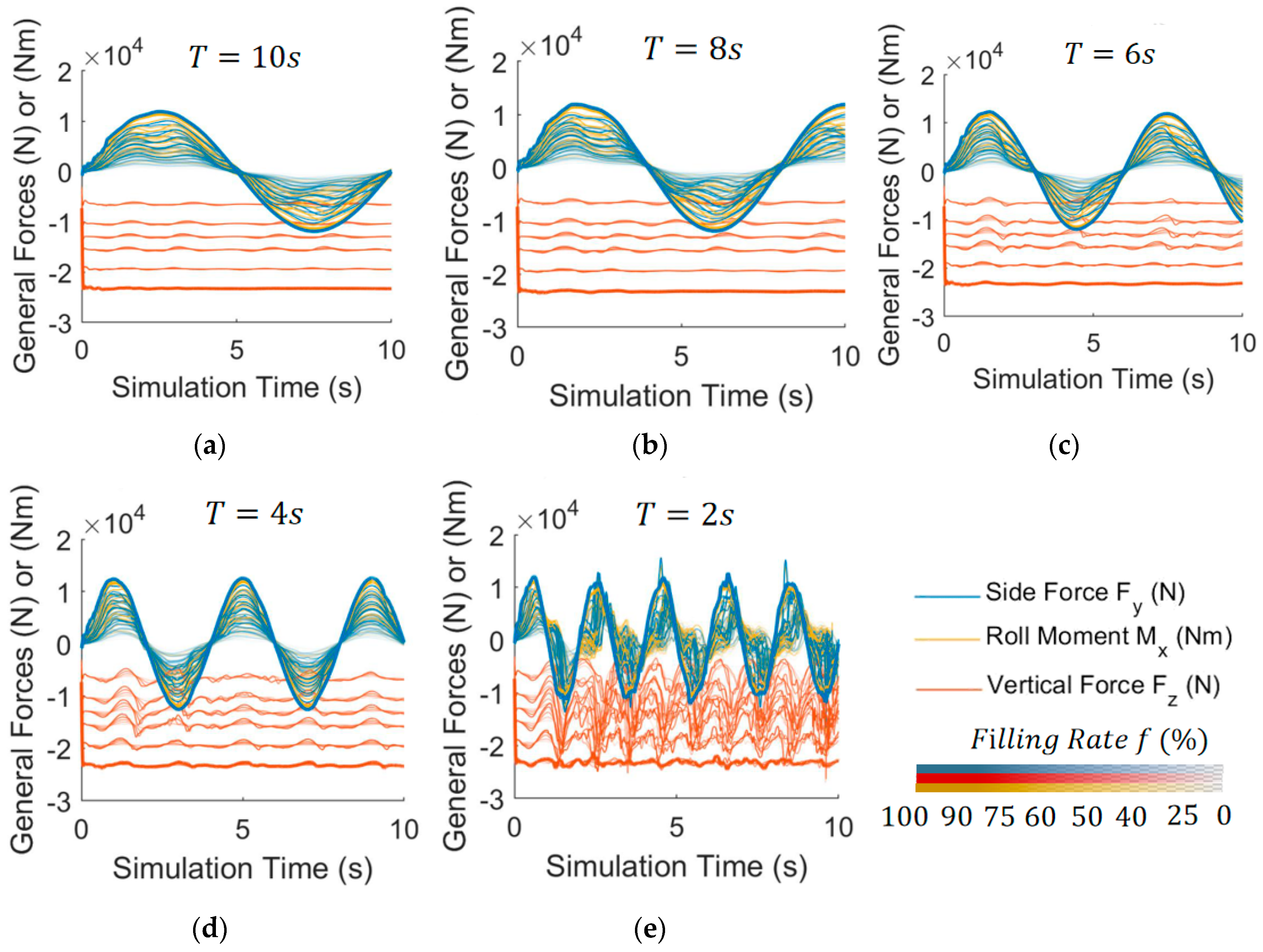
Figure 8.
Error map of SP, TP, TPSP and DMTP under orthogonal conditions of lateral acceleration excitation .(a.1–a.6) for SP Model under different filling rate; (b.1–b.6) for SP Model; (c.1–c.6) for TPSP Model; (d.1–d.6) for DMTP Model.
Figure 8.
Error map of SP, TP, TPSP and DMTP under orthogonal conditions of lateral acceleration excitation .(a.1–a.6) for SP Model under different filling rate; (b.1–b.6) for SP Model; (c.1–c.6) for TPSP Model; (d.1–d.6) for DMTP Model.
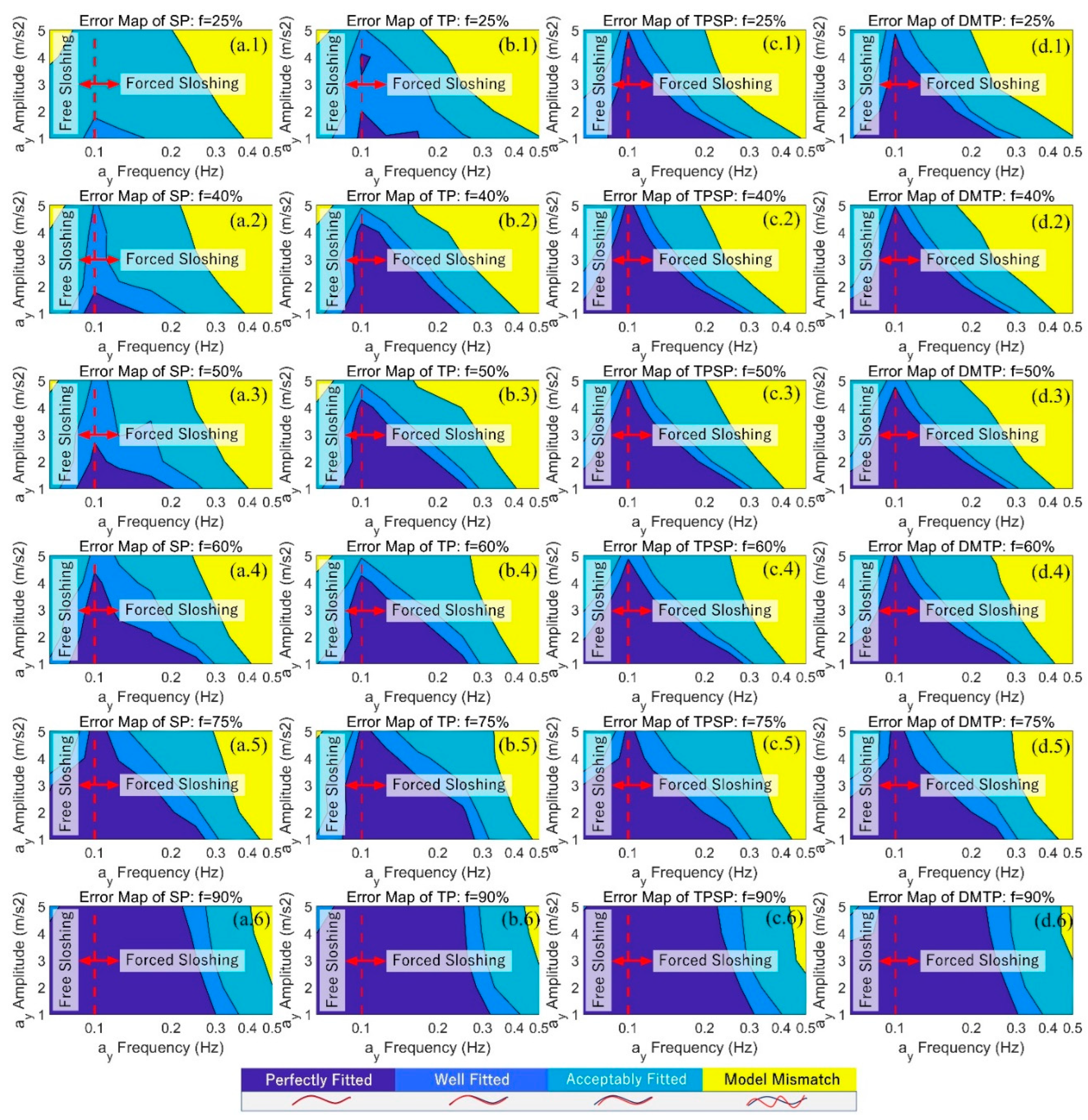
Figure 9.
Necessity for fluctuation sensor. (a) Fluid(pendulum) model related state variables are unavailable; (b) Error characteristics of open loop estimation.
Figure 9.
Necessity for fluctuation sensor. (a) Fluid(pendulum) model related state variables are unavailable; (b) Error characteristics of open loop estimation.
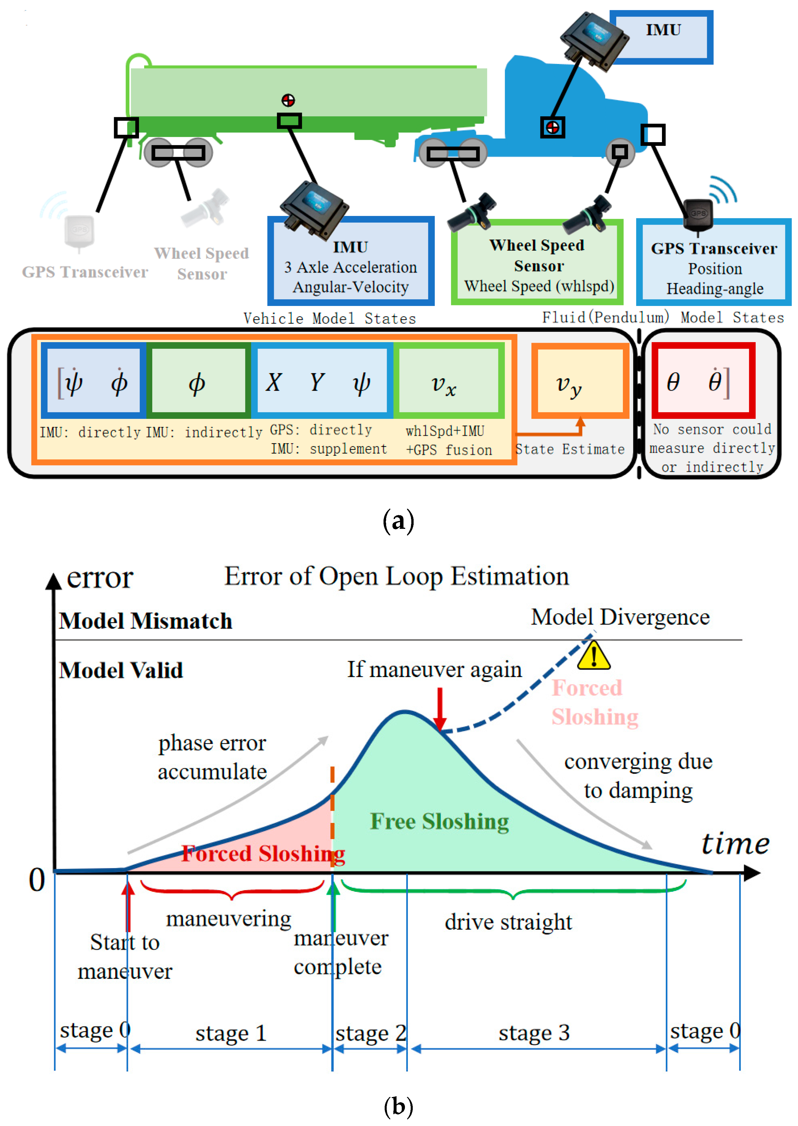
Figure 10.
Fluctuation sensor design. (a) Sensor assembly and example of use; (b) Measurement principle; (c) Sliding float board size considering measurement range; (d) Pulley block mechanism ensuring adaptive length adjustment.
Figure 10.
Fluctuation sensor design. (a) Sensor assembly and example of use; (b) Measurement principle; (c) Sliding float board size considering measurement range; (d) Pulley block mechanism ensuring adaptive length adjustment.
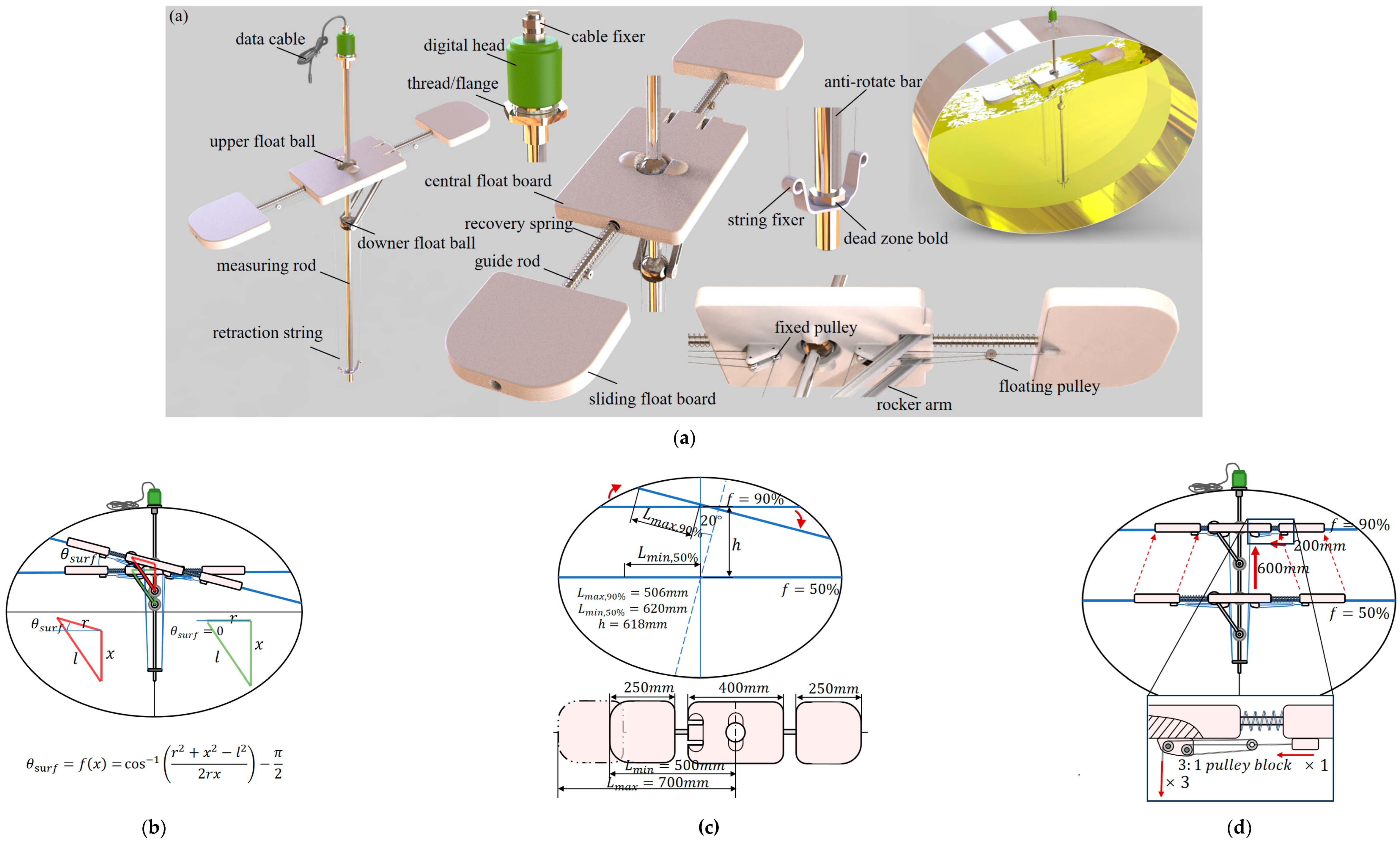
Figure 11.
Unscented Kalman filter based on DMTP and fluctuation sensor data.
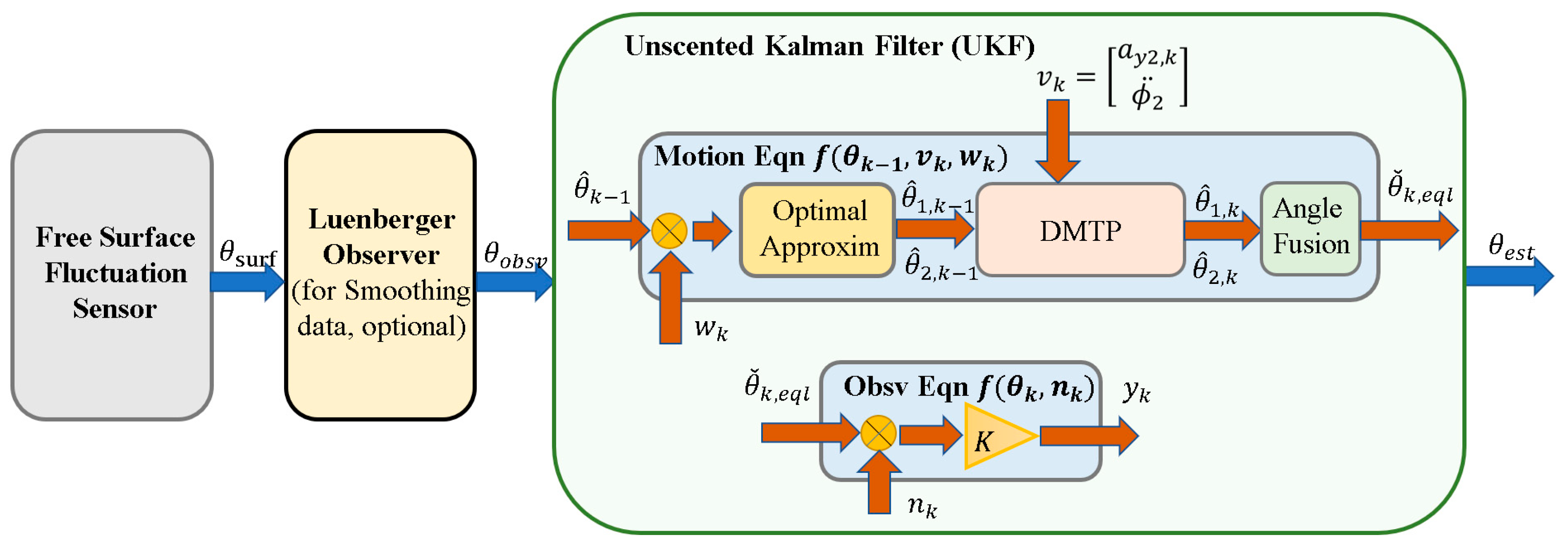
Figure 12.
Conversion method of DMTP to LSP. (a) Problem Description. (b) Center of Mass conversion method. (c) Convex combination method. (d) Verification in left cornering condition. (e) Verification in single lane change condition. (f) Verification in double lane change condition.
Figure 12.
Conversion method of DMTP to LSP. (a) Problem Description. (b) Center of Mass conversion method. (c) Convex combination method. (d) Verification in left cornering condition. (e) Verification in single lane change condition. (f) Verification in double lane change condition.
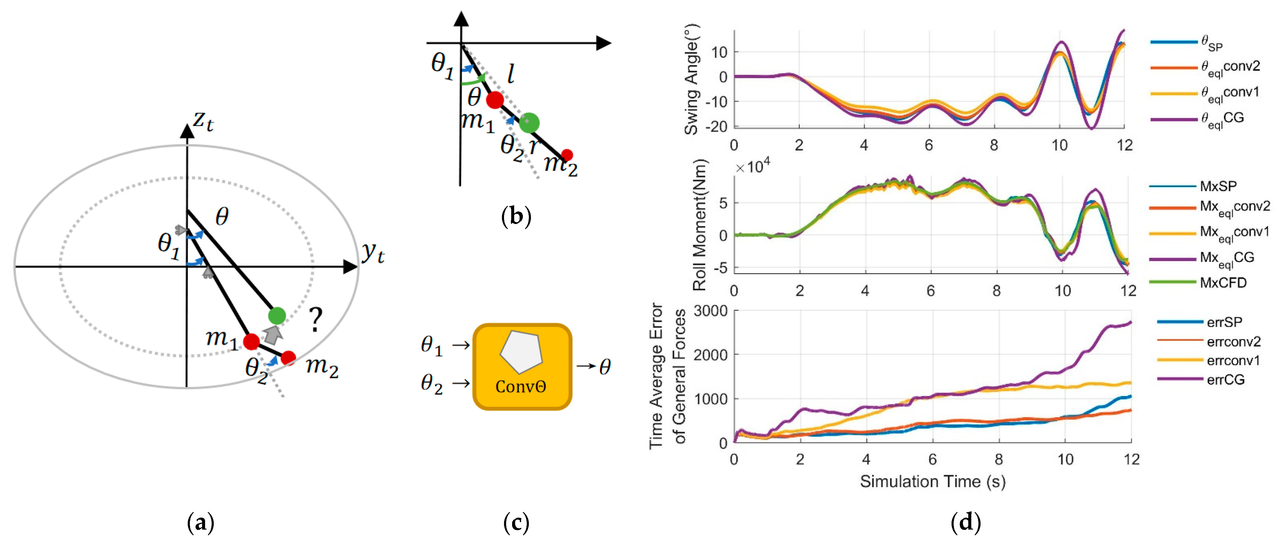
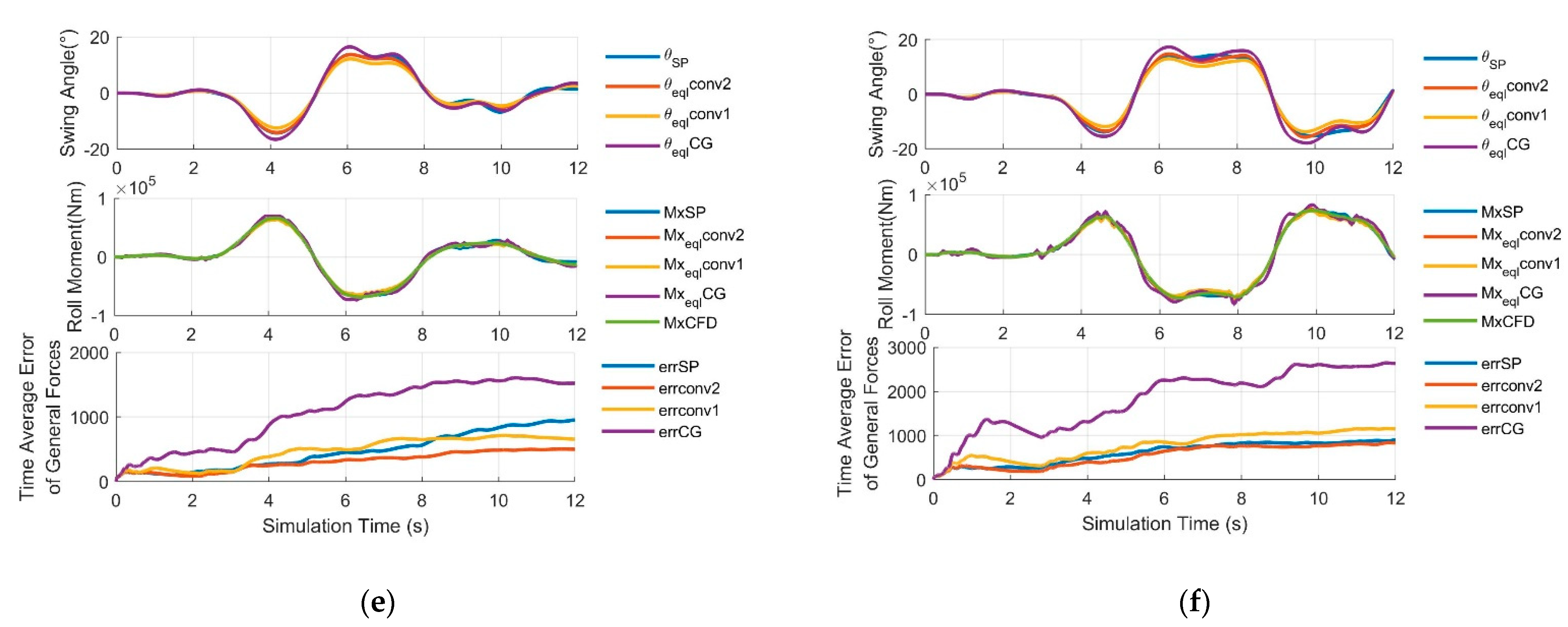
Figure 13.
Vehicle-fluid-co-simulation platform construction through bridging TruckSim and StarCCM+ by Matlab/Simulink.
Figure 13.
Vehicle-fluid-co-simulation platform construction through bridging TruckSim and StarCCM+ by Matlab/Simulink.
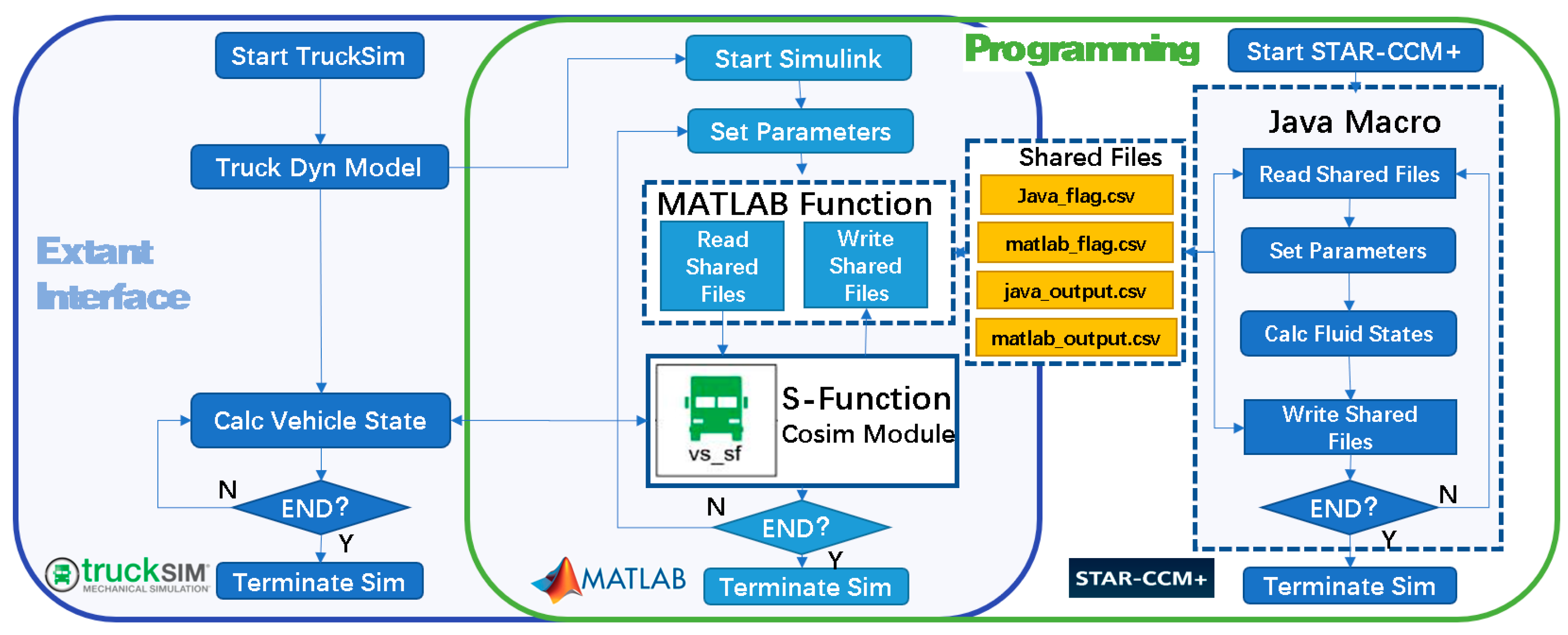
Figure 14.
Simulation model for verification of proposed observing method. (a) Vehicle-fluid-co-simulation module. (b) Sloshing observer.
Figure 14.
Simulation model for verification of proposed observing method. (a) Vehicle-fluid-co-simulation module. (b) Sloshing observer.
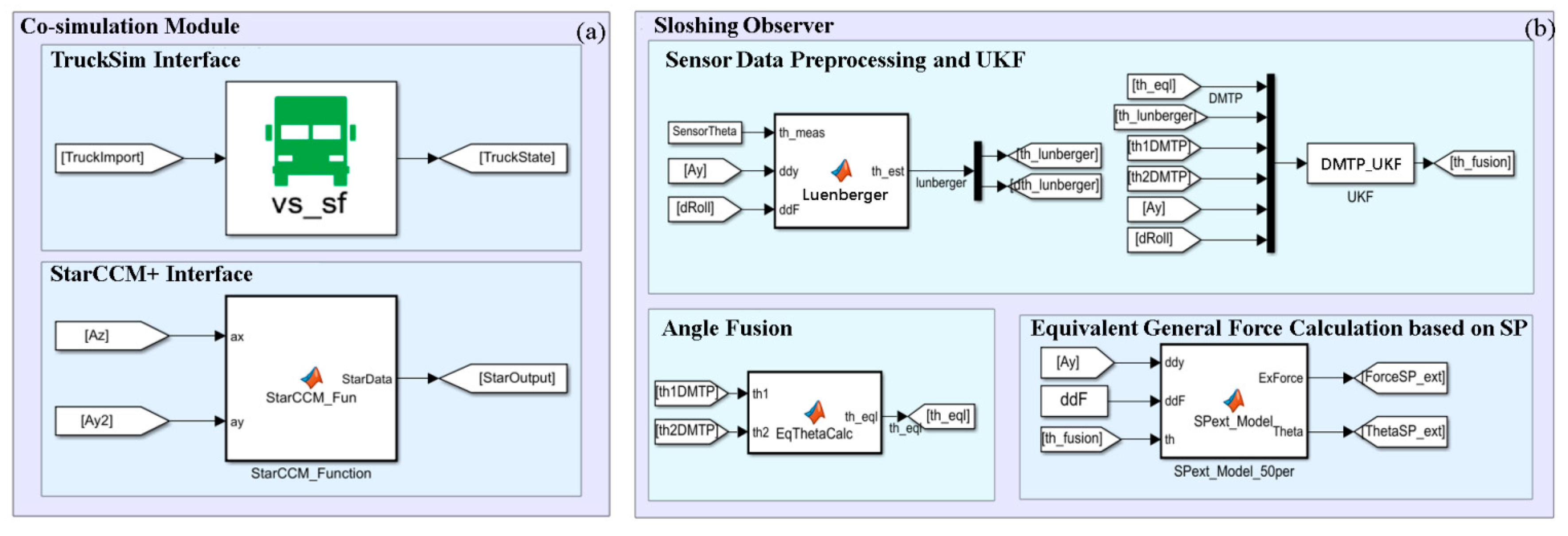
Figure 15.
Graphical processing method to simulate fluctuation sensor.
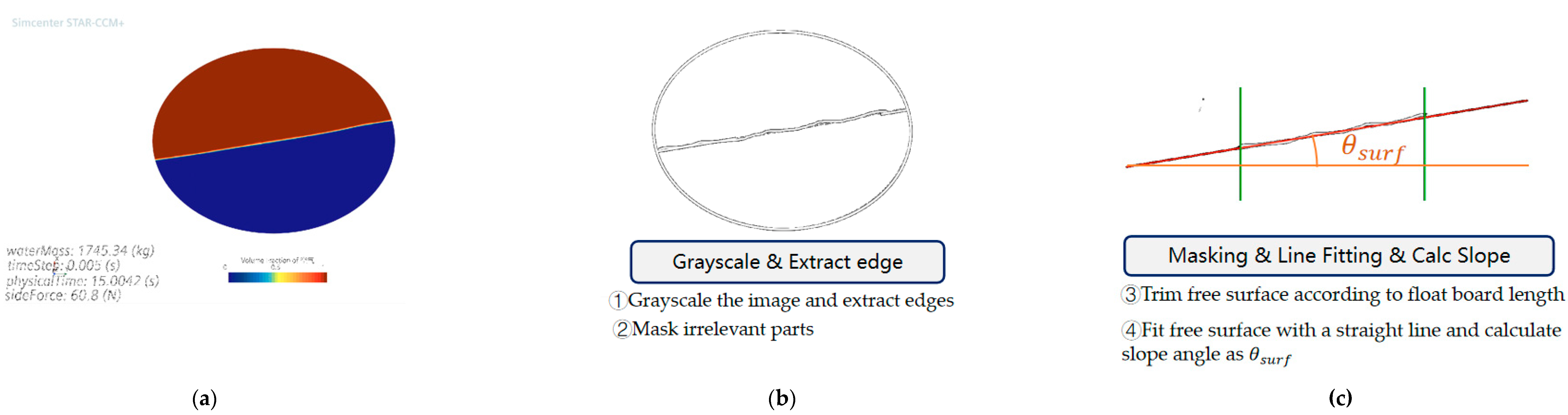
Figure 16.
Simulation of consecutive double lane change condition (CDLC). (a) CDLC introduction. (b) Trajectory following; (c) Observer input: lateral acceleration of trailer; (d) Observer input: rolling angular velocity of trailer; (e) Estimated swing angle ; (f) Estimated roll moment ; (g) Time average error of .
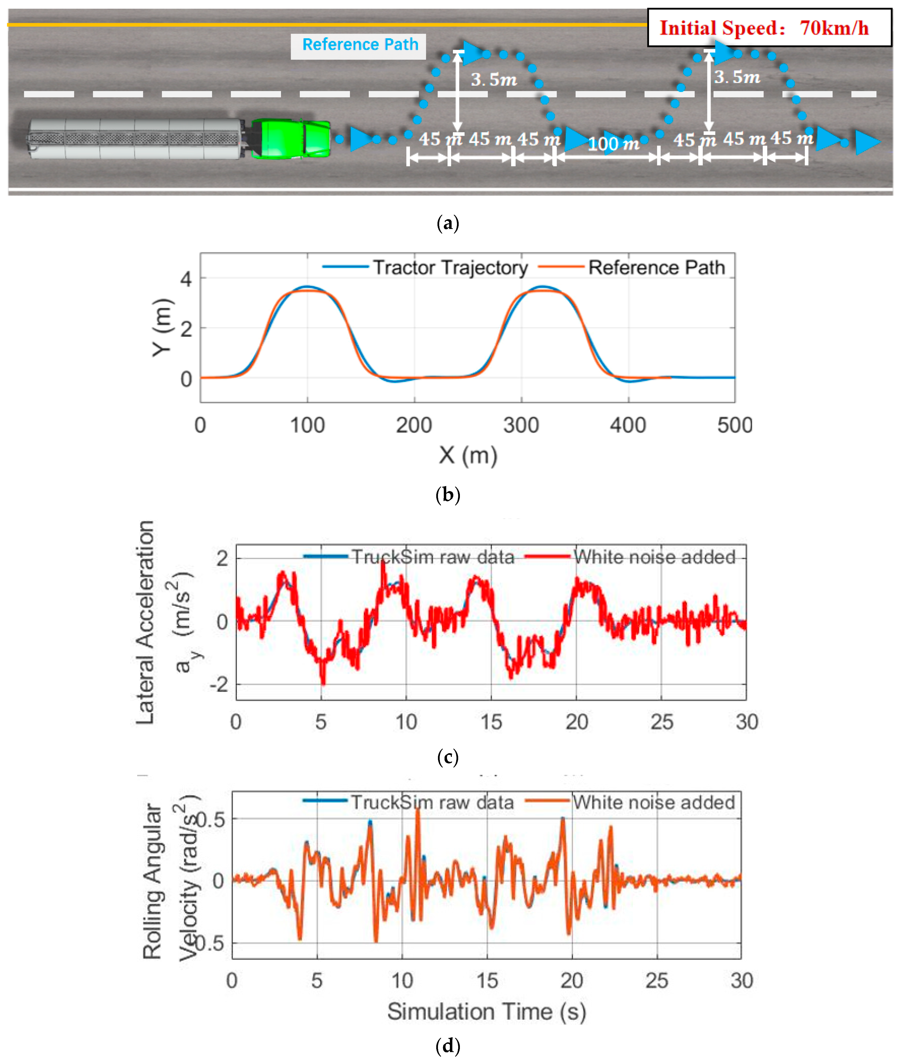
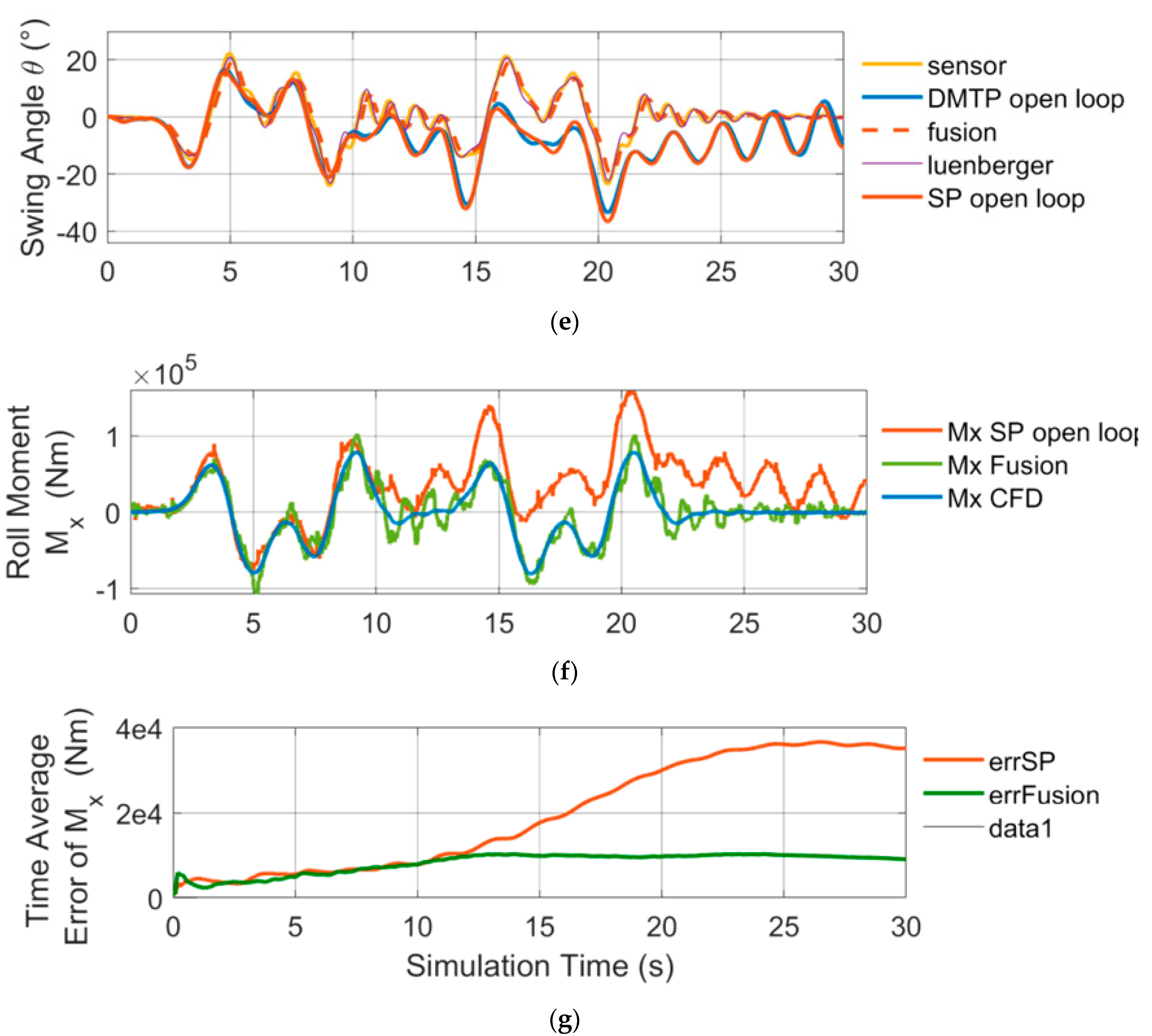

Table 1.
Spectral analysis of different sloshing models.
| Slosh Mode | 0 order | surface incline | 1st | 2nd | 3rd | higher order | ∞ |
|---|---|---|---|---|---|---|---|
| Model Name | |||||||
| Rigid body | √ | ||||||
| QS | √ | √ | |||||
| Linearized SP | √ | √ | √ | ||||
| SP/TP | √ | √ | √ | √ | √ | ||
| Multi-DOF Pendulum | √ | √ | √ | √ | √ | √ | |
| FVM-CFD | √ | √ | √ | √ | √ | √ | |
| Real Liquid | √ | √ | √ | √ | √ | √ | √ |
*: √ suggests the highest expressing ability of the model.
Disclaimer/Publisher’s Note: The statements, opinions and data contained in all publications are solely those of the individual author(s) and contributor(s) and not of MDPI and/or the editor(s). MDPI and/or the editor(s) disclaim responsibility for any injury to people or property resulting from any ideas, methods, instructions or products referred to in the content. |
© 2023 by the authors. Licensee MDPI, Basel, Switzerland. This article is an open access article distributed under the terms and conditions of the Creative Commons Attribution (CC BY) license (http://creativecommons.org/licenses/by/4.0/).
Copyright: This open access article is published under a Creative Commons CC BY 4.0 license, which permit the free download, distribution, and reuse, provided that the author and preprint are cited in any reuse.


