
Submitted:
29 August 2023
Posted:
18 September 2023
You are already at the latest version
Abstract
In this paper, we analyze the convergence of a finite difference method with the implicit forward time central space (FTCS) scheme for solving the three-dimensional advection-diffusion-reaction equation (ADRE). It is proved that the method is unconditionally convergent. We apply the scheme to obtain numerical solutions for the transport of pollutants in street tunnel problems with various reaction coefficients and various rates of change of concentrations of sources or sinks of pollution.
Keywords:
finite difference method
; convergence
; advection-diffusion-reaction equation
; pollutant concentration
1. Introduction
Advection-diffusion-reaction equations (ADRE) have been widely used as mathematical models in many areas of science and engineering, for example, in areas such as water pollution, air pollution, molecular diffusion, and chemical engineering. There are now many numerical methods that have been developed to solve linear and nonlinear ADREs. Some examples are as follows. In 2012, Diego et al [1] developed a model consisting of a decoupled system of advection-diffusion-reaction equations, along with the Navier-Stokes equations of incompressible flow, and solved the model by using the finite element method. In 2012, Savovic and Djordjevich [2] proposed an explicit finite difference method to solve a one-dimensional advection-diffusion equation with variable coefficients in semi-infinite media for three dispersion problems. In 2013, Appadu and Gidey [3] proposed two time-splitting procedures that they used to solve a 2D advection-diffusion equation with constant coefficients. In 2013, Bause and Schwegler [4] proposed a higher order finite element approximation for systems of coupled convection-dominated transport equations. In 2015, Mojtabi and Deville [5] proposed a finite element method to solve analytically using separation of variables and numerical solution of a time-dependent one-dimensional linear advection-diffusion equation with Dirichlet homogeneous boundary conditions and an initial sine function. In 2016, Gharehbaghi [6] proposed an explicit and an implicit differential quadrature method to compute a numerical solution of a one-dimensional time-dependent advection-diffusion equation with variable coefficients in a semi-infinite domain. In 2017, Gyrya and Lipnikov [7] proposed an arbitrary order mimetic finite difference discretization for the diffusion equation with non-symmetric tensorial diffusion coefficient in a mixed formulation on general polygonal meshes. In 2017, Bahar and Gurarslan [8] studied the effects of Lie-Trotter and Strang splitting methods on the solution of a one-dimensional advection-diffusion equation. In 2017, Oyjindal and Pochai [9] proposed models for numerical simulations of air pollution measurements near an industrial zone. The numerical experiments consisted of different conditions including normal and controlled emissions. The models were then solved using an explicit finite difference technique and the solutions were compared with the measurements for the controlled and uncontrolled point sources at the monitoring points. In 2018, Suebyat and Pochai [10] developed a three-dimensional air pollution measurement model for a heavy traffic area under a Bangkok sky train platform and used finite difference techniques to approximate the solutions. In 2018, Al-Jawary et al. [11] proposed a semi-analytical technique for finding the exact solutions for different types of Burger’s equations and systems of equations in 1D, 2D, and 3D. Also, the method was applied to solve the diffusion and advection-diffusion equations. In 2018, Kusuma et al. [12] proposed a finite difference (FTCS) method to solve a model of pollution distribution in a street tunnel using two dimensional advection and three dimensional diffusion in a rectangular box domain. In 2018, Lou et al. [13] developed reconstructed Discontinuous Galerkin methods for solving linear advection-diffusion equations on hybrid unstructured grids based on a first-order hyperbolic system formulation. In 2018, Bhatt et al, [14] developed a Krylov subspace approximation-based locally extrapolated exponential time differencing method and studied its accuracy and efficiency for solving three-dimensional nonlinear advection-diffusion-reaction systems. In 2020, Pananu et al. [15] analyzed the convergence of the finite difference method with the implicit forward time central space (FTCS) scheme for the two-dimensional advection-diffusion-reaction equation (ADRE) and applied the scheme to a pollutant dispersion with removal mechanism model in a reservoir. In 2020, Heng and Guodong [16] improved the element-free Galerkin method and used it for solving 3D advection-diffusion problems. In 2020, Cruz-Quintero and Jurado [17] proposed a backstepping design for the boundary control of a reaction-advection-diffusion equation with constant coefficients and Neumann boundary conditions. In 2021, Para et al. [18] proposed the characteristic finite volume method for solving a convection-diffusion problem on two-dimensional triangular grids and compared the accuracy of four piecewise linear reconstruction techniques on structured triangular grids, namely, Frink, Holmes-Connell, Green-Gauss, and least squares methods. In 2021, Hong et al. [19] discussed the numerical solution of 3D unsteady advection-diffusion equations using a meshless numerical scheme with a space-time backward substitution method. In 2021, Irfan and Hidayat [20] proposed a meshless finite difference method with B-splines for the numerical solution of coupled advection-diffusion-reaction problems. In 2021, Shahid et al [21] studied an epidemic type model with advection and diffusion terms for the transmission dynamics of a computer virus model with fixed population density. In 2021, García and Jurado [22] designed an adaptive boundary control for a parabolic type reaction-advection-diffusion PDE under the assumption of unknown parameters for both advection and reaction terms and Robin and Neumann boundary conditions. In 2022, Para et al. [23] proposed an explicit characteristic-based finite volume method (FVM) for the numerical solution of advection-diffusion-reaction equations (ADRE) and applied it to solve some 1D and 2D water pollution problems which can be modeled in terms of ADREs. Then, the FVM results were compared with numerical results obtained using a finite difference method (FDM) with an implicit forward time central space (FTCS) scheme.
In this article, we consider the application of a finite difference method based on the implicit forward time central space (FTCS) scheme to the numerical solution of an advection-diffusion-reaction equation of the following form:
where is a scalar quantity, is a given advection velocity vector, is a diffusion coefficient, is a reaction coefficient, is a prescribed source term, is a position vector and time , where . The present paper is organized as follows. The convergence theory is briefly provided in Section 2. The consistency and stability analysis and numerical results of the method are given in Section 3. Using the method, numerical results and their graphs for the air pollution problems written in terms of the ADRE in Eq. (1) are shown in Section 4. The conclusion of our work is presented in Section 5.
2. Convergence Theory
We consider the following initial time, space boundary value problem (IBVP) for the advection-diffusion-reaction equation
where , and with the initial time condition
and either Dirichlet or Neumann boundary space conditions
In Eqs. (2)–(4), T is a finite time, is the boundary of the spatial domain , and are given functions, is an advection vector, is a diffusion coefficient, is a reaction constant and is a source term. In addition, L is a linear partial differential operator from a space of continuous functions F to a space of continuous functions H, where the dependent variable , and where and .
The first step in developing the finite difference method is to discretize , and . We assume that there are step sizes of length in the x direction, step sizes of length in the y direction and step sizes of length in the z direction. For simplicity, we will assume that and therefore , and . Then the discretized version of is the spatial grid
where , , . The boundary of the spatial grid is
Similarly, the interval is discretized with N step sizes of size . The set of discretized times is then
Finally, we define and as discretized function spaces with domain . We also define a projection of the exact solution of (2) onto and a projection of the source term onto .
We can then write a finite difference scheme (FDS) corresponding to the continuous partial differential equation (2) in the form
where is a finite difference operator, corresponding to the partial differential operator L, which acts from the discrete function space to the discrete function space . The initial condition in (3) can then be rewritten as the discretized initial condition
and, for the Dirichlet case, the boundary conditions in (4) can be rewritten as the discretized boundary conditions
Lax’s equivalence theorem [24]
An initial time, space boundary value problem (IBVP) is called a properly posed IBVP if it has a unique solution. In this paper, all advection-diffusion-reaction equations that we study will be properly posed IBVP.
Then Lax’s equivalence theorem states that necessary and sufficient conditions for the solution of a finite difference approximation to converge to the unique solution of the IBVP are the following conditions of convergence, consistency and stability.
Using the definition given above of the projection of a function in the continuous space H onto the discrete space , we define the truncation error (T.E.) between the finite difference system Eq. (8) and the IBVP Eq. (2) as follows
Introducing the norm in the set of discrete functions as the infinity norm
we have the definition of convergence for numerical methods as follows
Definition 1.
Convergence
Definition 2.
Convergence with order m
The FDS in Eq. (8) converges with order m if
where C is a positive constant that does not depend on h.
1) Consistency : A finite difference representation of a PDE is said to be consistent [24] if the difference between the PDE and its difference representation vanishes as the mesh is refined, i.e.,
Definition 3.
where C is a positive constant that does not depend on h.
2) Stability : The finite difference scheme defined by (8) with linear operator will be called stable, if there exists such that for arbitrary and for
the solution of the FDS, in Eq. (8), exists and is unique and satisfies the inequality
where the positive constant C does not depend on h.
The inequality (17) has to be true for any initial conditions and source terms of Eq. (2). In particular, if , then the condition (17) reduces to the necessary condition for stability of the homogeneous version of (8).
For the special case of Fourier or Von Neumann Analysis [24], a solution of the FDS (8) for can be written in the form
where , and are wave numbers and are eigenfunctions corresponding to eigenvalues of . The necessary condition for stability of FDS (8) for will then hold for all if the following inequality holds:
3. Consistency and Stability Analysis
Consider the following initial-boundary value problem
in which the above partial differential equation is the component form of (1). Here is the dependent variable and is the advection velocity where and w are the velocities in the x-, y- and z-directions, respectively.
In this section, we will analyze the convergence of the finite difference method with the implicit FTCS scheme applied to (20). We discretize the domain of the problem: , where the spatial grid is defined in (5) and the time grid has points with
Following the method in Section 2, we use Lax’s equivalence theorem to prove the convergence of the FTCS by proving its consistency and stability. We first show the consistency of the FTCS. The implicit FTCS scheme of Eq. (20) is as follows.
where and .
The truncation error for (22) obtained using the method is
Therefore, from (24), we have
Taking , then we have
We will now prove the stability of the finite difference method with the implicit FTCS scheme for numerical solution of (20). In order to illustrate stability of the method, we initially show that condition (19) holds for the homogeneous equation of (22) and then that condition (17) is satisfied for the nonhomogeneous equation (22). For convenience, we set .
Case I: Homogeneous equation
Setting in equation (22), we obtain the discretized homogeneous version of (22). Assuming a discretized solution of the resulting equation as , [24], we obtain the following equation for the eigenvalue
Then, we can solve (25) for the eigenvalue as follows.
Letting and , we then obtain,
Consequently, the magnitude of is
Therefore, condition (19) for Von Neumann stability, which is independent of and h, has been proved.
Case II: Nonhomogeneous equation
We now prove that condition (17) is satisfied for the nonhomogeneous equation (22) with by finding a solution for the linear system of difference equations (22) and (23) if is assumed known. Substituting and in (22) and (23), we obtain
After rearranging, we can rewrite (26) in the form
and where the step sizes and h can be chosen so that the coefficients satisfy the conditions
Lemma 1.
If the coefficients of Eq.(28) satisfy the conditions Eq.(29) then the solution of Eq.(28) exists and is unique and satisfies the inequality
Proof
First, we prove inequality (30). Assume that .
Let . Then
This completes the proof.
Now we will prove the stability of the implicit FTCS scheme by showing that inequality (17) is satisfied.
Proof
Let , and be the smallest non-negative integers such that
where Now let be the discretized boundary set of J, i.e.,
It is obvious that if then we have
If then replacing in (26) with we obtain
Next we make the following hypothesis:
Without loss of generality we assume that and further assume that the hypothesis (H1) holds. We can estimate the right side of (34) as
Then, substituting (36) into the right hand side of (34), we obtain
Therefore,
where We now establish the following inequality representing the maximum principle as
We will now prove that for the given initial and boundary conditions in (27), the maximum solution
is bounded for all for finite .
At time , the maximum is .
Then, from (39), the maximum at time is
Similarly, the maximum at time is
Then, by iteration we find that the maximum at time is
and the maximum at time is
Then, as in Eq. (16), for , we can define
The above inequality is true for all , and hence we have that
Hence, inequality (17) is satisfied and the solution is stable. This completes the proof.
4. Numerical Results
In this section, we use the implicit forward time central space (FTCS) finite difference method to solve two cases (homogeneous and nonhomogeneous) of three-dimensional ADRE problems of air pollution. In three dimensions, the advection-diffusion-reaction equation can be written as follows:
where [kg/m] is the air pollutant concentration at [m] and time t s, u, v, w are wind velocity components [m/s] in , and directions, respectively, and are constant diffusion coefficients in the horizontal direction [m/s], is a constant diffusion coefficient in the direction (vertical) [m/s], R is a reaction coefficient, and is the rate of change of concentrations of sources or sinks of air pollutants [kg/ms].
In this section, we use an implicit forward time central space (FTCS) scheme to solve the problems. Using the results from section 2, we can write the finite diference equation as
We assume that the initial condition is
and that the boundary conditions are as shown in Table 1.
After rearrangement, we can rewrite (48) in the form
where
Case 1 : We consider the three-dimensional advection-diffusion equation (47). By taking and this reduces to a two-dimensional advection three-dimensional diffusion equation for transport of pollutants in the street tunnel problem discussed in [12,25]
This system of partial differential equation and initial condition (49) and boundary condition Table 1 comes from a model of pollution distribution in a street tunnel, where the wind flows steadily in the x and y directions and there is no flux of pollutant through the solid side-walls or the solid base and roof of the tunnel. We use the nondimensionalised parameters and time . The numerical solutions and the contour plots of the problem obtained using the implicit FTCS scheme in Eq. (48) are plotted in Figure 1, Figure 2, Figure 3 and Figure 4. We have tested the accuracy of our numerical solutions by comparing them with that of Kusuma et al [12] and found that there was good agreement.
Case 2: In this problem, We consider the three-dimensional advection-diffusion equation (47). By taking and with a decay rate (R) and source term (Q). The advection-diffusion-reaction equation that we consider is as follows.
This case of partial differential equation and initial condition (49) and boundary condition Table 1 comes from a model of pollution distribution in a street tunnel, where the wind flows steadily in the x and y directions and there is no flux of pollutant through the solid side-walls or the solid base and roof of the tunnel. We use the nondimensionalised parameters and time .
We have computed the numerical solutions of the above system using the implicit FTCS method for the following cases.
- and . The results for this case are shown in Figure 5 (a) - (d) at a height meters for and , respectively.
- and . The results for this case are shown in Figure 6 (a) - (d) at a height meters for and , respectively.
- and . The results for this case are shown in Figure 7 (a) - (d) at a height meters for and , respectively.
- m for and . The results for this case are shown in Figure 8 (a) at m and (b) at m.
- m for and . The results for this case are shown in Figure 9 (a) at m and (b) at m.
It can be seen that the numerical solutions for the different Q and R values show similar qualitative behavior but with differences in detail.
5. Conclusions
In this work, we have studied a finite difference method (FDM) for obtaining numerical solutions of advection-diffusion-reaction equations (ADRE) and applied the methods to solve air pollutant problems. For the finite difference method we have used the implicit forward time central space (FTCS) scheme. For the applications, we have solved 3-D air pollutant concentration problems for tunnels. We have investigated the stability, consistency and convergence of the finite difference method. We applied the implicit FTCS finite difference method to solve 3-D ADRE models for three problems of air pollution in tunnels for a range of different source terms Q and reaction terms R. For case 1, we checked the accuracy of our solutions by comparing them with previously published results. We assumed that , that there was advection in the x and y directions and diffusion in the x, y and z directions. We then compared our numerical solutions of with Kusuma et al [12] and found that there was good agreement. For case 2, we assumed that Q and R were non-zero, that there was advection in the and direction and diffusion in the x, y and z directions. We found that the effects of the Q and R were to rapidly reduce the pollutant concentrations in the tunnel.
Author Contributions
Conceptualization, S.S., K.P., E.J.M., S.S. and S.P.; methodology, S.S., K.P., E.J.M., S.S. and S.P.; software, S.S., K.P. and E.J.M.; validation, S.S., K.P. and E.J.M.; formal analysis, S.S., K.P., E.J.M. and S.S.; writing-review and editing, S.S., K.P. and E.J.M. All authors have read and agreed to the published version of manuscript.
Funding
The research was funded by Faculty of Applied Science, King Mongkut’s University of Technology North Bangkok, Thailand contract no. 661132.
Acknowledgments
The authors would like to express their sincere thanks to the Department of Mathematics, Faculty of Applied Science at King Mongkut’s University of Technology North Bangkok for supporting us to do this research.
Conflicts of Interest
The authors declare no conflict of interest.
References
- Di Pietro, D.A.; Ern, A. Mathematical Aspects of Discontinuous Galerkin Methods 2012.
- Savović, S.; Djordjevich, A. Finite difference solution of the one-dimensional advection–diffusion equation with variable coefficients in semi-infinite media. International Journal of Heat and Mass Transfer 2012, 55, 4291–4294. [Google Scholar] [CrossRef]
- Appadu, A.R.; Gidey, H. Time-splitting procedures for the numerical solution of the 2D advection-diffusion equation. Mathematical Problems in Engineering 2013, 2013. [Google Scholar] [CrossRef]
- Bause, M.; Schwegler, K. Higher order finite element approximation of systems of convection–diffusion–reaction equations with small diffusion. Journal of computational and applied mathematics 2013, 246, 52–64. [Google Scholar] [CrossRef]
- Mojtabi, A.; Deville, M.O. One-dimensional linear advection–diffusion equation: Analytical and finite element solutions. Computers & Fluids 2015, 107, 189–195. [Google Scholar]
- Gharehbaghi, A. Explicit and implicit forms of differential quadrature method for advection–diffusion equation with variable coefficients in semi-infinite domain. Journal of Hydrology 2016, 541, 935–940. [Google Scholar] [CrossRef]
- Gyrya, V.; Lipnikov, K. The arbitrary order mimetic finite difference method for a diffusion equation with a non-symmetric diffusion tensor. Journal of Computational Physics 2017, 348, 549–566. [Google Scholar] [CrossRef]
- Bahar, E.; Gürarslan, G. Numerical solution of advection-diffusion equation using operator splitting method. International Journal of Engineering and Applied Sciences 2017, 9, 76–88. [Google Scholar] [CrossRef]
- Oyjinda, P.; Pochai, N. Numerical Simulation to Air Pollution Emission Control near an Industrial Zone. Advances in Mathematical Physics 2017, 2017. [Google Scholar] [CrossRef]
- Suebyat, K.; Pochai, N. Numerical Simulation for a Three-Dimensional Air Pollution Measurement Model in a Heavy Traffic Area under the Bangkok Sky Train Platform. Abstract and Applied Analysis. Hindawi, 2018, Vol. 2018.
- Al-Jawary, M.A.; Azeez, M.M.; Radhi, G.H. Analytical and numerical solutions for the nonlinear Burgers and advection–diffusion equations by using a semi-analytical iterative method. Computers & Mathematics with Applications 2018, 76, 155–171. [Google Scholar]
- Kusuma, J.; Ribal, A.; Mahie, A.G. On FTCS Approach for Box Model of Three-Dimension Advection-Diffusion Equation. International Journal of Differential Equations 2018, 2018. [Google Scholar] [CrossRef]
- Lou, J.; Li, L.; Luo, H.; Nishikawa, H. Reconstructed discontinuous Galerkin methods for linear advection–diffusion equations based on first-order hyperbolic system. Journal of Computational Physics 2018, 369, 103–124. [Google Scholar] [CrossRef]
- Bhatt, H.; Khaliq, A.; Wade, B. Efficient Krylov-based exponential time differencing method in application to 3D advection-diffusion-reaction systems. Applied Mathematics and Computation 2018, 338, 260–273. [Google Scholar] [CrossRef]
- Pananu, K.; Sungnul, S.; Sirisubtawee, S.; Phongthanapanich, S. Convergence and Applications of the Implicit Finite Difference Method for Advection-Diffusion-Reaction Equations. IAENG International Journal of Computer Science 2020, 47, 645–663. [Google Scholar]
- Cheng, H.; Zheng, G. Analyzing 3D advection-diffusion problems by using the improved element-free Galerkin method. Mathematical Problems in Engineering 2020, 2020. [Google Scholar] [CrossRef]
- Cruz-Quintero, E.; Jurado, F. Boundary Control for a Certain Class of Reaction-Advection-Diffusion System. Mathematics 2020, 8, 1854. [Google Scholar] [CrossRef]
- Para, K.; Jitsom, B.; Eymard, R.; Sungnul, S.; Sirisubtawee, S.; Phongthanapanich, S. An accuracy comparison of piecewise linear reconstruction techniques for the characteristic finite volume method for two-dimensional convection-diffusion equation. ZAMM-Journal of Applied Mathematics and Mechanics/Zeitschrift für Angewandte Mathematik und Mechanik 2021, 101, e201900245. [Google Scholar] [CrossRef]
- Sun, H.; Xu, Y.; Lin, J.; Zhang, Y. A space-time backward substitution method for three-dimensional advection-diffusion equations. Computers & Mathematics with Applications 2021, 97, 77–85. [Google Scholar]
- Hidayat, M.I.P. Meshless finite difference method with B-splines for numerical solution of coupled advection-diffusion-reaction problems. International Journal of Thermal Sciences 2021, 165, 106933. [Google Scholar] [CrossRef]
- Shahid, N.; Rehman, M.A.u.; Khalid, A.; Fatima, U.; Shaikh, T.S.; Ahmed, N.; Alotaibi, H.; Rafiq, M.; Khan, I.; Nisar, K.S. Mathematical analysis and numerical investigation of advection-reaction-diffusion computer virus model. Results in Physics 2021, 26, 104294. [Google Scholar] [CrossRef]
- Murillo-García, O.F.; Jurado, F. Adaptive Boundary Control for a Certain Class of Reaction–Advection–Diffusion System. Mathematics 2021, 9, 2224. [Google Scholar] [CrossRef]
- Para, K.; Sungnul, S.; Sirisubtawee, S.; Phongthanapanich, S. A Comparison of Numerical Solutions for Advection-Diffusion-Reaction Equations between Finite Volume and Finite Difference Methods. Engineering Letters 2022, 30. [Google Scholar]
- Tannehill, J.C.; Anderson, D.; Pletcher, R.H. Computational Fluid Mechanics and Heat Transfer, 2nd ed.; Taylor & Francis, 1997. [Google Scholar]
- Thongmoon, M.; McKibbin, R.; Tangmanee, S. Numerical solution of a 3-D advection-dispersion model for pollutant transport. Thai Journal of Mathematics 2012, 5, 91–108. [Google Scholar]
Figure 1.
Pollutant distribution (a) and contour plot (b) for case 1 in a street tunnel with advection only in x and y directions at .
Figure 1.
Pollutant distribution (a) and contour plot (b) for case 1 in a street tunnel with advection only in x and y directions at .
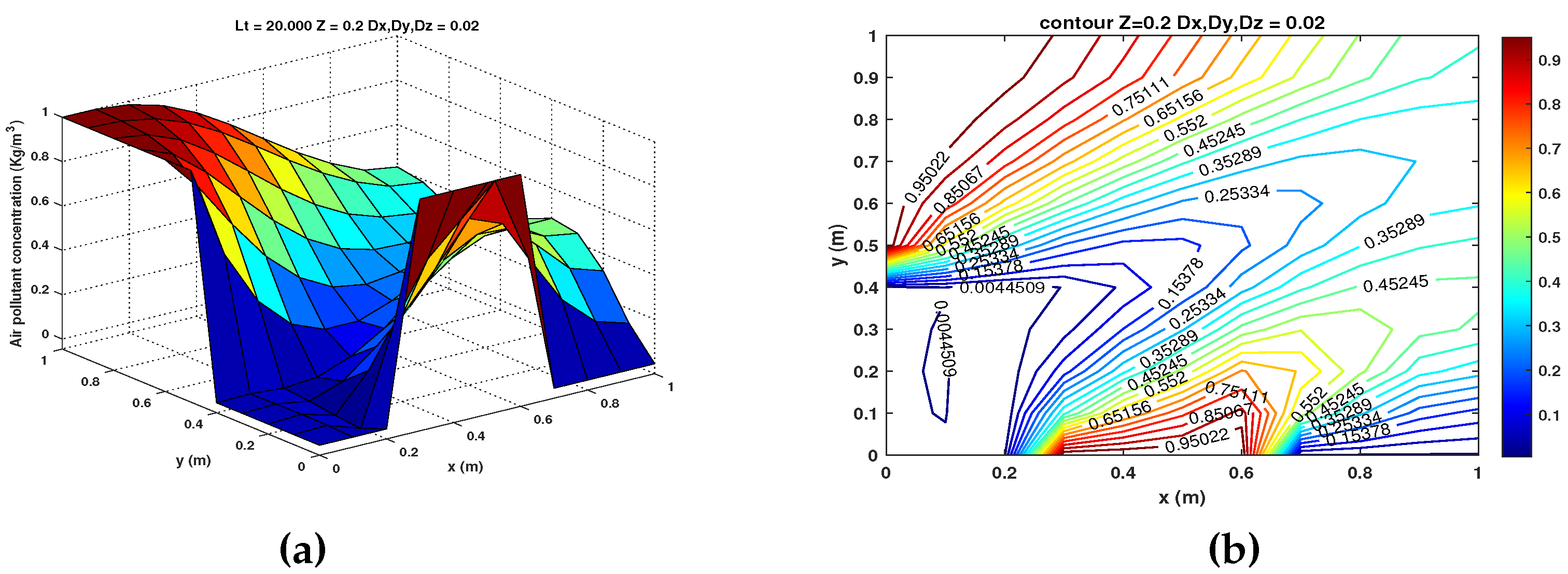
Figure 2.
Pollutant distribution (a) and contour plot (b) for case 1 in a street tunnel with advection only in x and y directions at .
Figure 2.
Pollutant distribution (a) and contour plot (b) for case 1 in a street tunnel with advection only in x and y directions at .
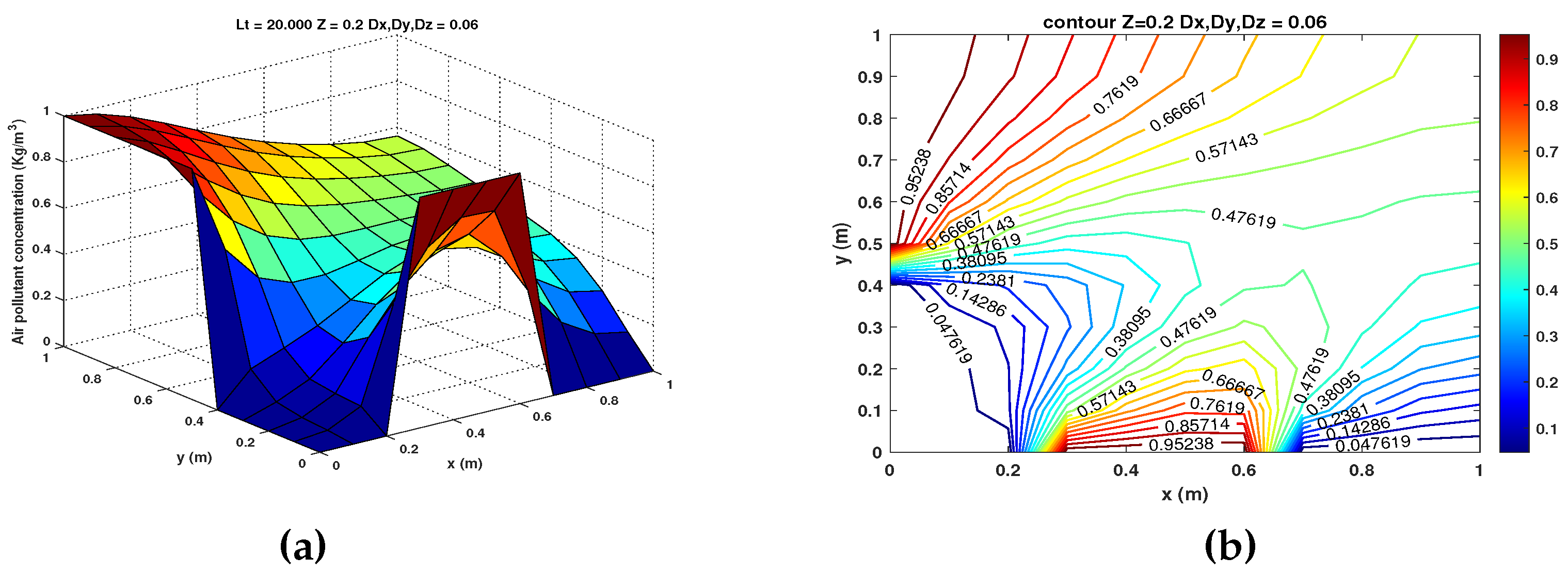
Figure 3.
Pollutant distribution (a) and contour plot (b) for case 1 in a street tunnel with advection only in x and y directions at .
Figure 3.
Pollutant distribution (a) and contour plot (b) for case 1 in a street tunnel with advection only in x and y directions at .
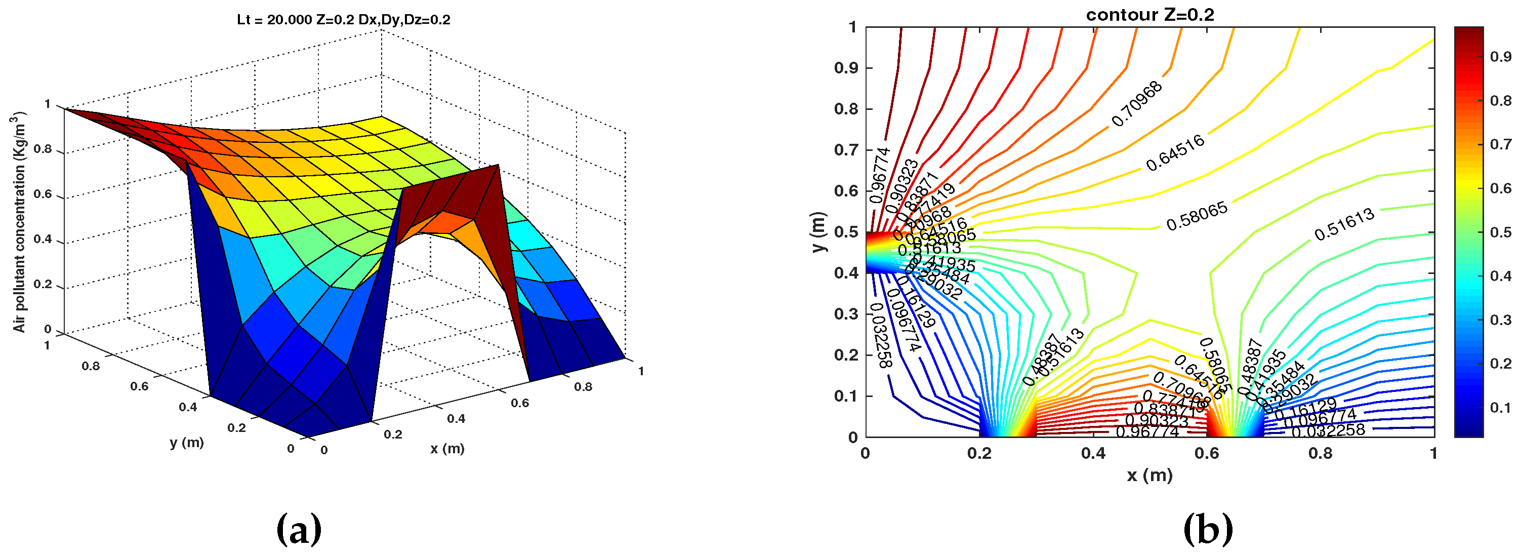
Figure 4.
Pollutant distribution (a) and contour plot (b) for case 1 in a street tunnel with advection only in x and y directions at .
Figure 4.
Pollutant distribution (a) and contour plot (b) for case 1 in a street tunnel with advection only in x and y directions at .
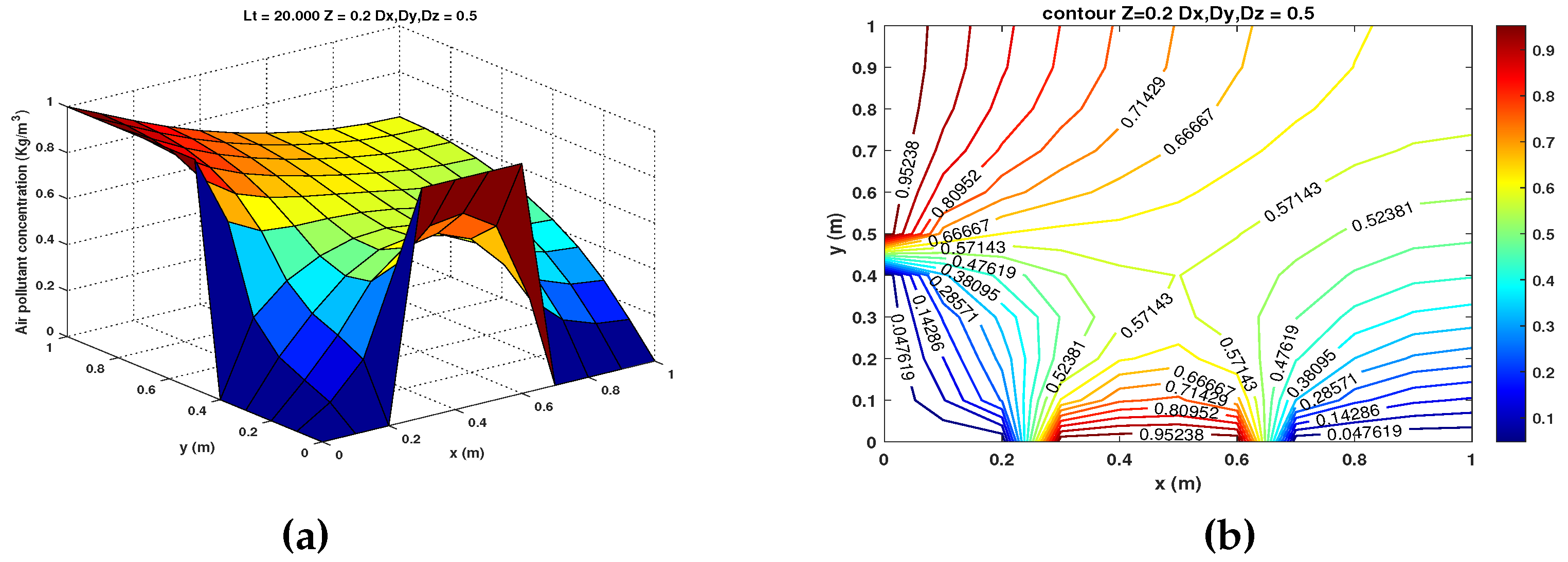
Figure 5.
Numerical solution of air pollutant concentration and contour plot for case 2 for and (a) , (b) , (c) and (d) .
Figure 5.
Numerical solution of air pollutant concentration and contour plot for case 2 for and (a) , (b) , (c) and (d) .
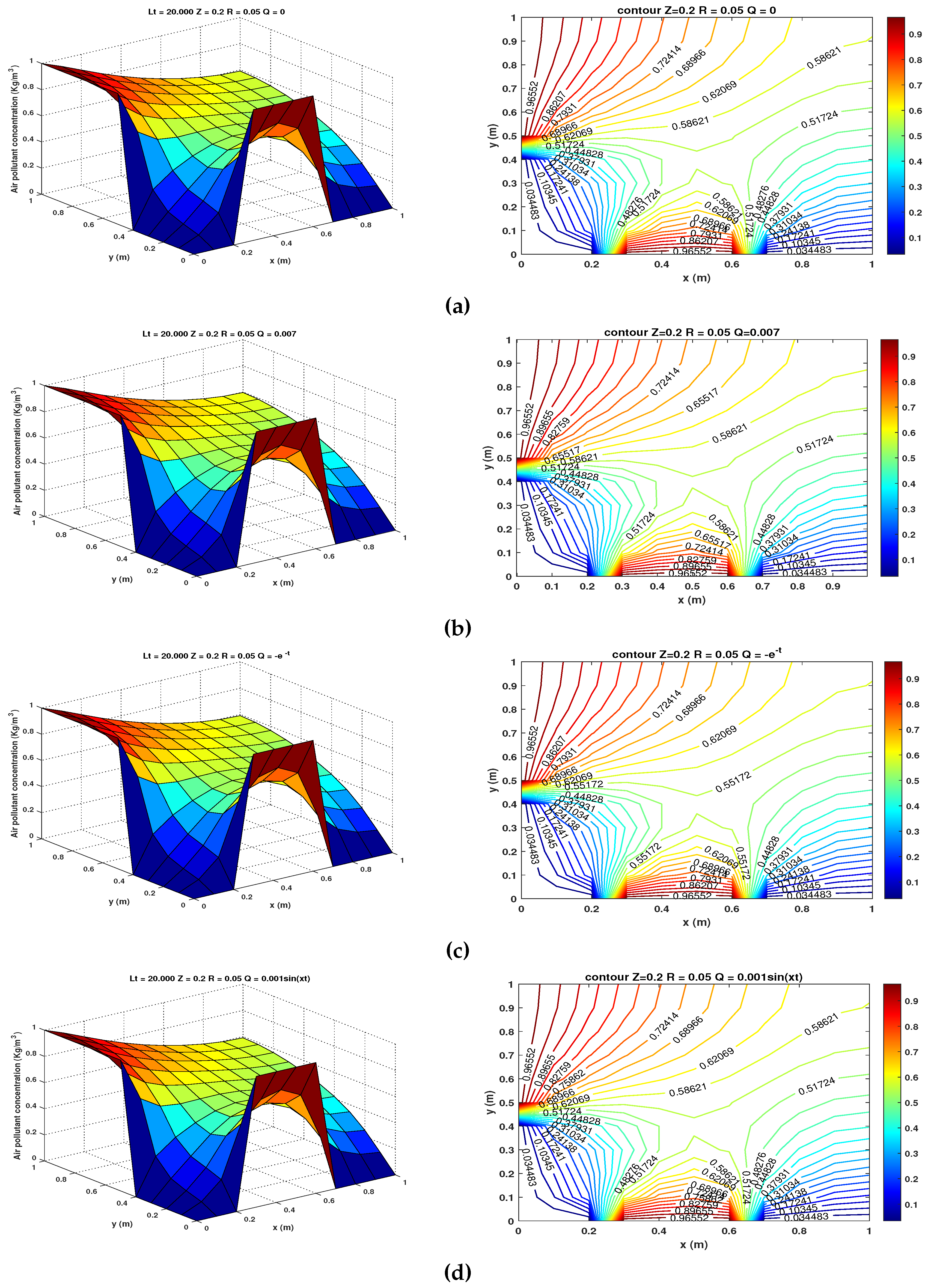
Figure 6.
Numerical solution of air pollutant concentration and contour plot for case 2 for and (a) , (b) , (c) and (d) .
Figure 6.
Numerical solution of air pollutant concentration and contour plot for case 2 for and (a) , (b) , (c) and (d) .
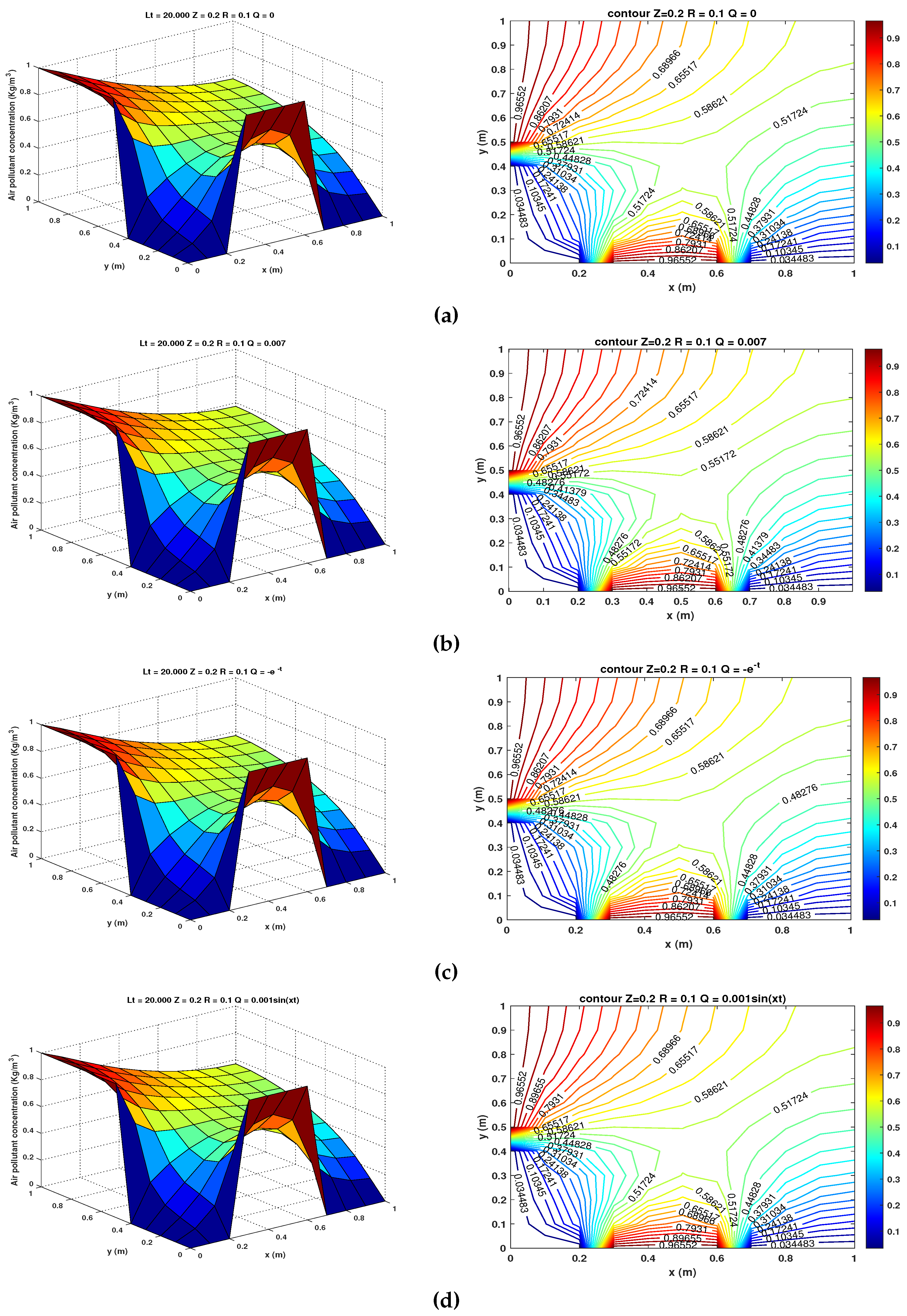
Figure 7.
Numerical solution of air pollutant concentration and contour plot for case 2 for and (a) , (b) , (c) and (d) .
Figure 7.
Numerical solution of air pollutant concentration and contour plot for case 2 for and (a) , (b) , (c) and (d) .
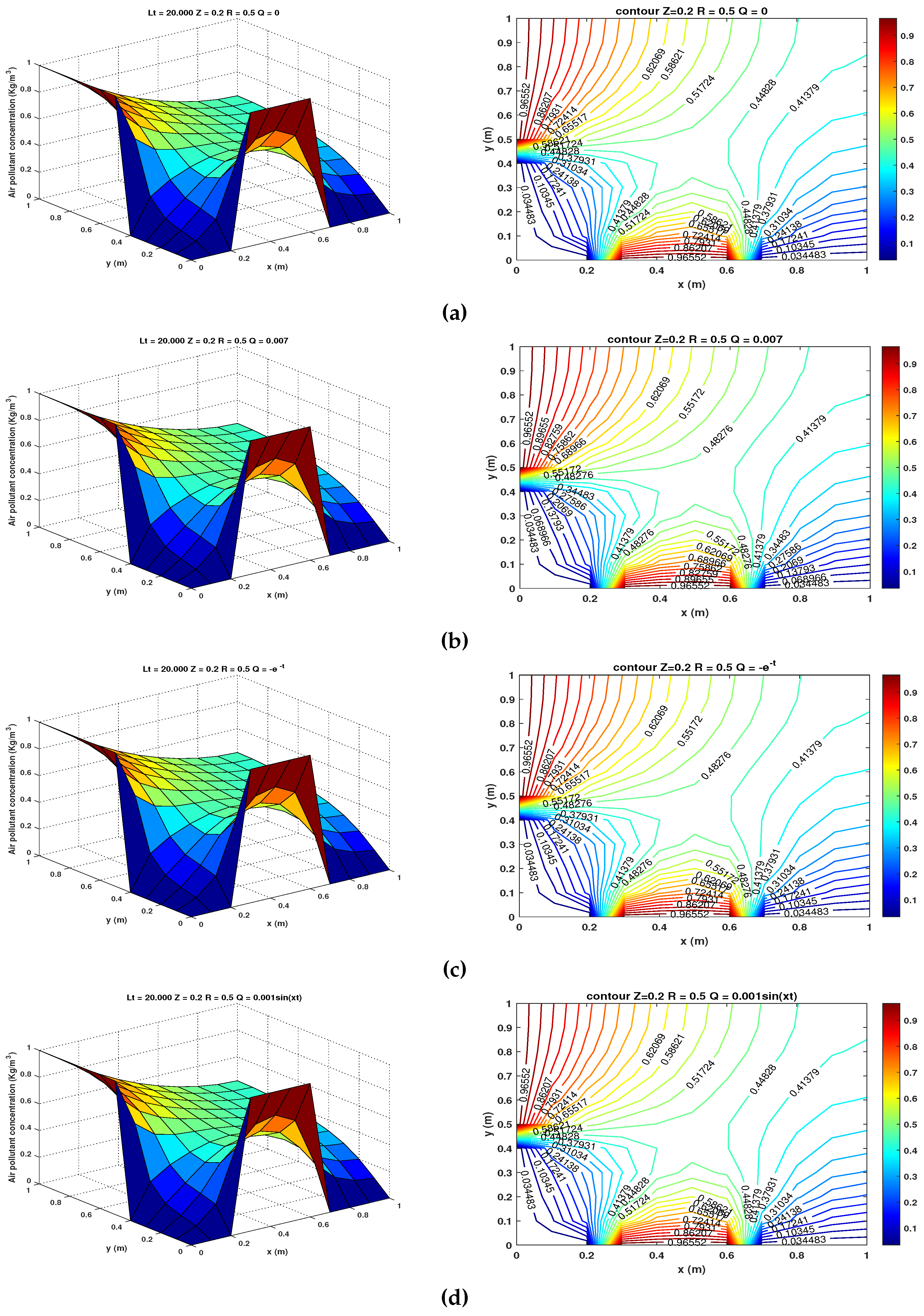
Figure 8.
Comparison of numerical solutions for Case 2 at m for and at (a) m and (b) m.
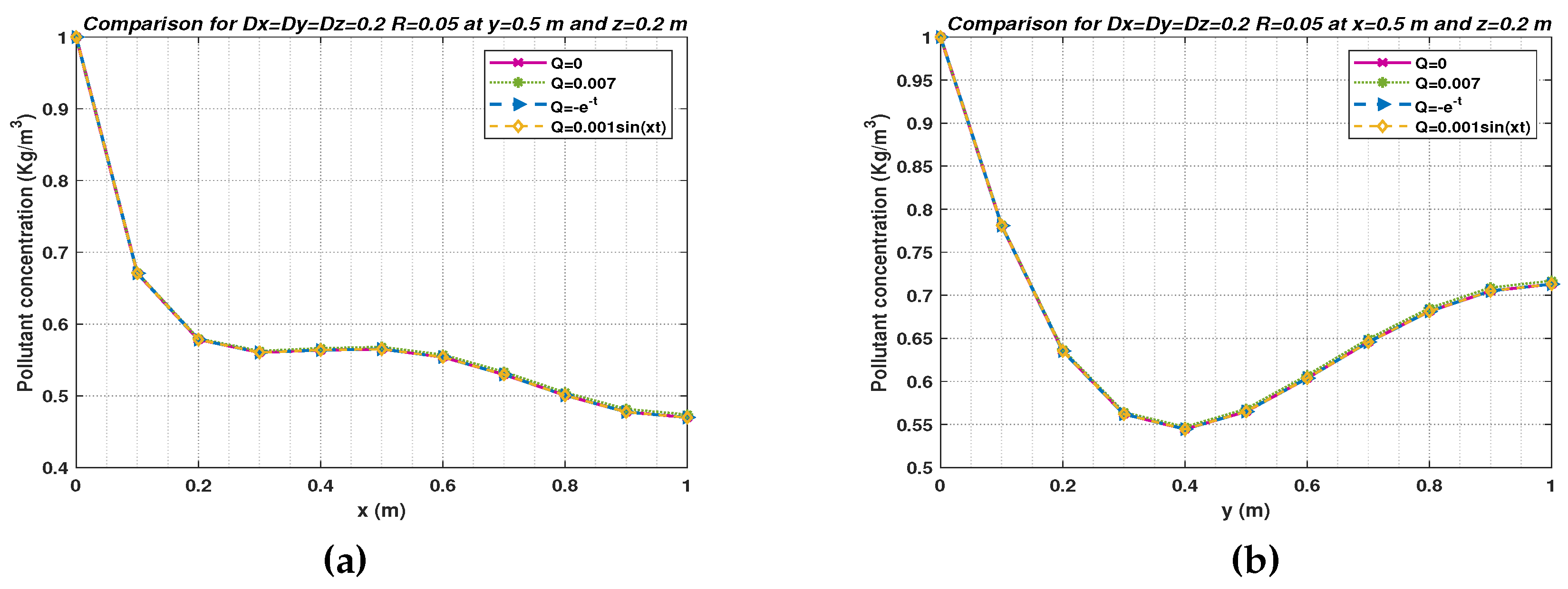
Figure 9.
Comparison of numerical solutions for Case 2 at m for of at (a) m and (b) m.
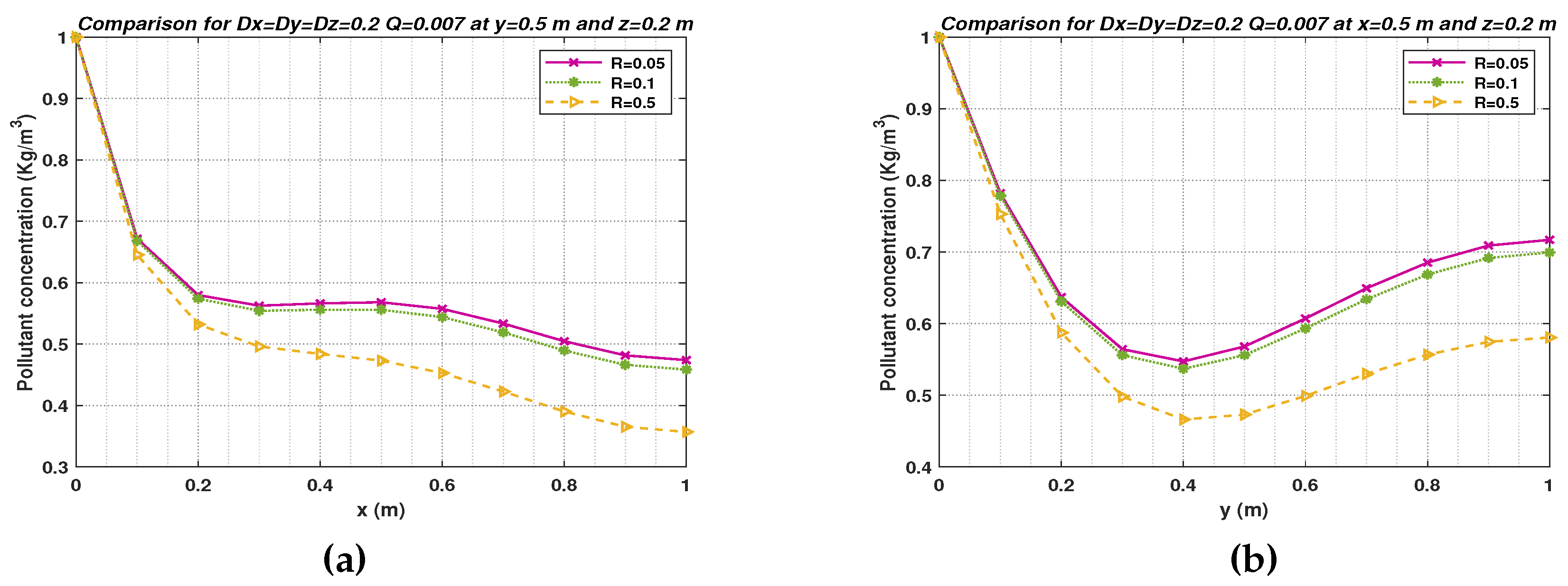

Table 1.
Boundary conditions.
| Boundary | Boundary condition | Value |
|---|---|---|
| Entrance gate : | 0 | |
| Entrance gate : | 1 | |
| Exit gate : | 0 | |
| Right side wall : | 0 | |
| Right side wall : | 1 | |
| Right side wall : | 0 | |
| Left side wall : | 0 | |
| Ground : | 0 | |
| Ceiling : | 0 |
Disclaimer/Publisher’s Note: The statements, opinions and data contained in all publications are solely those of the individual author(s) and contributor(s) and not of MDPI and/or the editor(s). MDPI and/or the editor(s) disclaim responsibility for any injury to people or property resulting from any ideas, methods, instructions or products referred to in the content. |
© 2023 by the authors. Licensee MDPI, Basel, Switzerland. This article is an open access article distributed under the terms and conditions of the Creative Commons Attribution (CC BY) license (http://creativecommons.org/licenses/by/4.0/).
Copyright: This open access article is published under a Creative Commons CC BY 4.0 license, which permit the free download, distribution, and reuse, provided that the author and preprint are cited in any reuse.


