Introduction
Civil engineering construction has grown in popularity in recent decades. Advanced technologies are utilized to protect critical civil engineering structures from terrorist attacks. Finite element modelling (FEM) is taken into consideration in practice since a special effort needs to be made to conduct experimental examination on steel studs subjected to blast loading. Because of their integrated qualities, cold-formed steel stud walls offer a strong resistance to blast loading. They have very good energy absorption, ductility and stiffness. In thin-walled members, tension membrane action was good. In blast resistance design thin-walled structure is one of the better solutions for moderate blast (Bondok et al., 2015). Cold-formed steel sections are very thin, designed dimensions of these sections have very good resistivity against local buckling. The high strength and cost efficiency is one of the foremost advantages of cold-formed steel section and also highly preferred in Australian countries (Kesawan & Mahendran, 2018). In 2001, steel structure was collapsed by an air crash explosion and the estimated strain rate was 1000 S-1 in USA (Ritchie, Packer, Zhao, et al., 2017). To safeguard the human lives from blast loading, there are two important structural considerations to be made such as maintaining the structural integrity and shielding the occupant from debris fog. The solution for those condition is the formation of exterior steel stud wall. The objective of stud wall is to limit the deformation and absorb more kinetic energy from threat level (DiPaolo & Woodson, 2006). In blast resistant design, one of the major parameters is toughness. It is used to determine the energy absorption and plastic behavior of structure. Stud should resist huge pressure and it can dissipate the energy to other components. To increase the resistivity of stud, various parameters such as connection type, fastener detail, sheathing material property and stud thickness should be considered. FEA is essential to evaluate the resistivity of stud against blast. In the cold-formed steel stud wall systems, the strength and stiffness were investigated. Type of sheathing material and fasteners are also the major parameters to influence the stud wall stiffness (Vieira & Schafer, 2012) .To avoid the premature failure of the members and connections, various sheathing material such as oriented strand board, gypsum board were used to absorb the energy (Static response evaluation of cold-formed steel stud walls. MS thesis). The response of blast loaded cold-formed steel sections mainly depends upon the connections, track, stud, sheathing material (B. M. Agee 2010 & T. R. McWilliam 2012). The bending capacity of channel section is also decided by its moment of inertia. At the same time, the moment of inertia is not constant throughout the span of section. Thus, the yield of section may vary and deformation is high in some locations (Salim et al., 2005) (H. Salim & P.Muller, 2005). High complexity is observed to conduct experimental investigations on infill stud walls. The experimental methods were available in limited numbers only. The alternative option is to conduct full scale test in static vacuum chamber. Vacuum is created inside the chamber and uniform pressure is applied on the specimen. The response of the members can be recorded by data acquisition system. It is one of the best sources to conduct test under excessive loading (Salim et al., 2005) .An emphasis was made on connection between stud and track and found that stud utilize the full moment capacity and highly ductile during the application of dynamic load. It is recommended to provide anchor system in the connection. Tension membrane behavior can be created by using additional screws in the connection. In the blast resistant design, the wall should have sufficient ductility and it should resist excessive deformation. The involvement of ductility in stud wall system is adequate for yielding of connection and for high energy absorption capacity. A hemispherical-shaped TNT charge was employed in two tests in the experimental study, the first weighing 1,000 kg and the second 500 kg with a standoff distance 27m and 15 m respectively. When subjected to impulsive loading, the field-tested cold-formed RHS parts functioned admirably due to their high ductility. The additional mass is primarily owing to the changed cross section; however, a small amount of the increased mass is attributable to extended cladding pieces (Ritchie, Packer, Seica, et al., 2017). The geometric proportions of the CFS studs influence the performance of the sheathing board. The strength and method of failure of the sheathing-fastener connection can both be considerably influenced by the type of screw/fastener utilized for the sheathing installation. Self-drilling fasteners with rubber washers must be used in the installation of CFS sheathed wall panels to prevent hard bearing on the sheathing owing to pulling force (Siva Ganesh Selvaraj et al., 2019). Ballistic pendulums have long been used to determine the impulse or energy applied by explosives. It is obvious that increasing the number of carbon fiber layers results in increased energy absorption. (Langdon et al., 2007). In this current study, cold-formed steel channel section with web corrugations was investigated in detail. Corrugation acts as an energy absorber. The mass of TNT used as 1.56kg and the thickness of stud was varied from 1.19 mm to 1.5mm. The models were analyzed using finite element analysis and displacement was one of the major outputs. These results were validated using Artificial neural network and response surface method. Finally, the regression value decides the accuracy of output from FE analysis.
Finite element analysis
Cold-formed steel sheets of various thickness and material properties (Whelan et al., 2016) were used (as shown in
Table 1) in the present study. The sheets which were fabricated as stud, top track, bottom track, verti clip, buckle bridge. Hot rolled steel bolts were used in the stud wall system.
Non-linear analysis was caried out using Dynamic Explicit using ABAQUS. Therefore, the NLGOM (Non- linear Geometry) was switched on during the analysis. The plastic material properties of the structural components were taken from the earlier research as given in
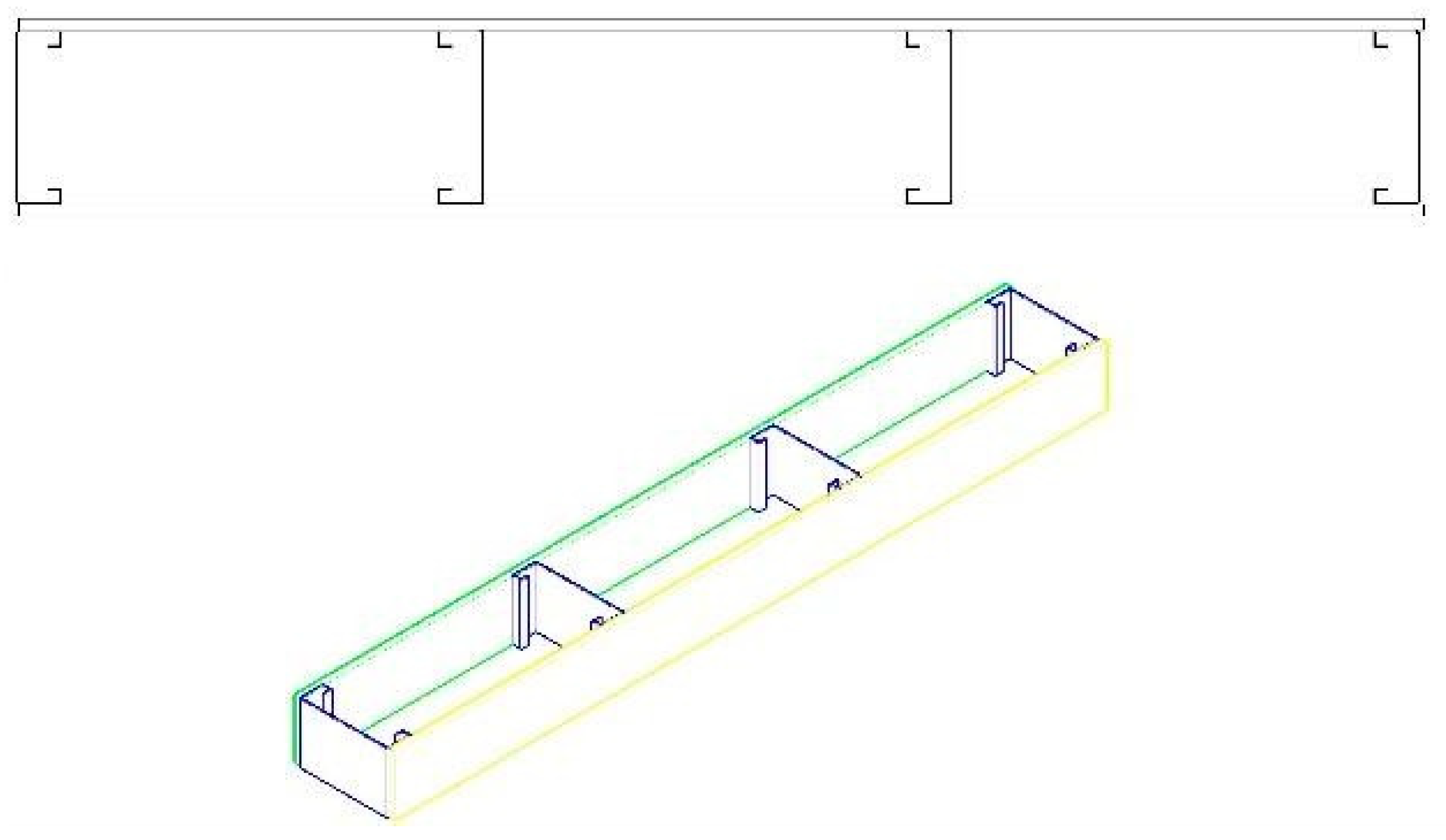
Table 2. Mass scaling concept was used to carry over finite element analysis. The total running time of the model is 10 milliseconds. According to the mass scaling, the results were captured for every 0.5 milliseconds. The orientation of stud in wall assembly of both models as shown in
Figure 1.
Validation using Experimental Program of Whelan et al., 2016
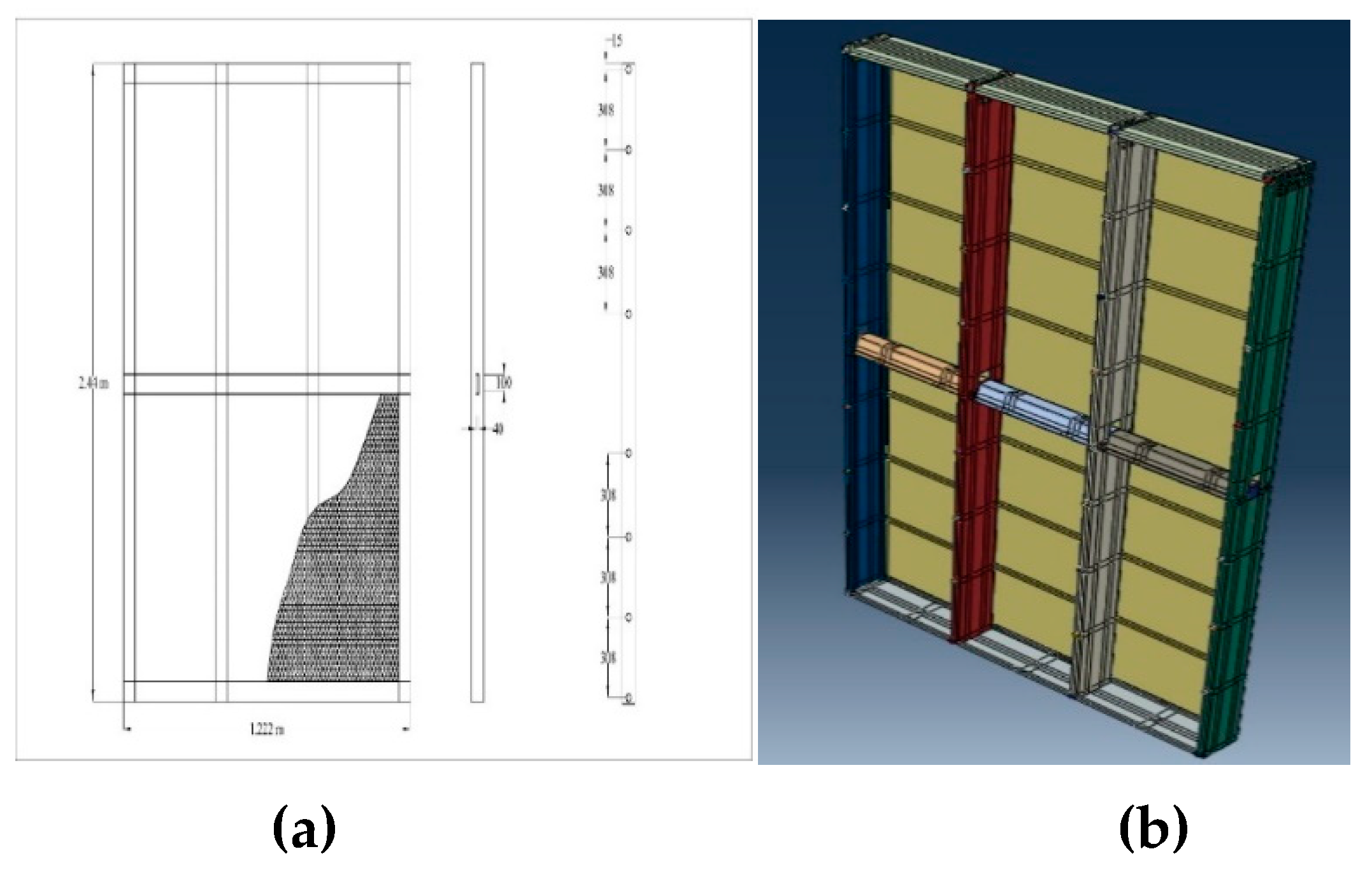
Whelan et al., 2016 conducted an experimental investigation of cold-formed steel stud wall (
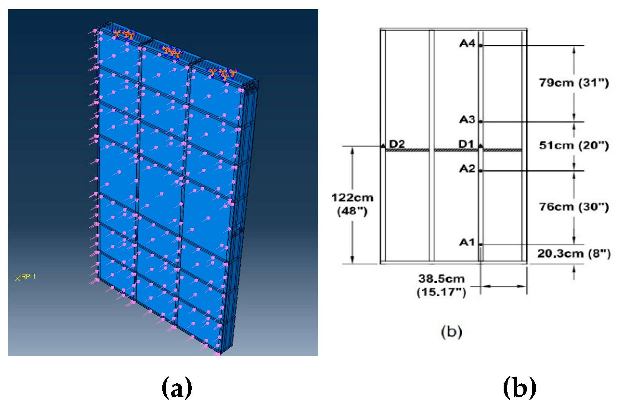
Figure 2(a)) under blast loading. The stud wall specimen consists of track, stud, solid rod, buckle bridge, verti clip, self-drilling screw (of diameter 10 mm). The connections between stud and track are screw connection. The length of screw depends on the connection location. In this study, a stud wall was subjected to explosion. It is an open-air blast experiment. The three identical specimens of cold-formed steel stud wall with a dimension of 2.440 m height and 1.220 m width were tested. The equivalent weight of TNT and the scaled distances are the parameters. Four studs are acting as vertical component and two tracks are acting as horizontal component. The lateral stiffness of the wall under blast was enhanced by the buckle bridge system placed at the mid height of the wall. In experimental set up, both tracks were connected by a bolted arrangement with the reaction frame. Computational modelling was used with the boundary condition of stud wall (shown in
Figure 2(b)). The material properties of the components were assigned for the model.
Influence of stud shapes
The shape of cold-formed steel stud plays a dynamic role in failure mechanism of wall. In comparison with conventional structure, the connection element such as self-tapping screw was affected due to premature failure. Therefore, understanding the behaviour of stud shape is an essential process to carry over to make the structural connection to withstand the various loading conditions (Luis Laim et al., 2022). It was observed that the Sigma shapes of cold-formed steel can withstand the temperature up to 600
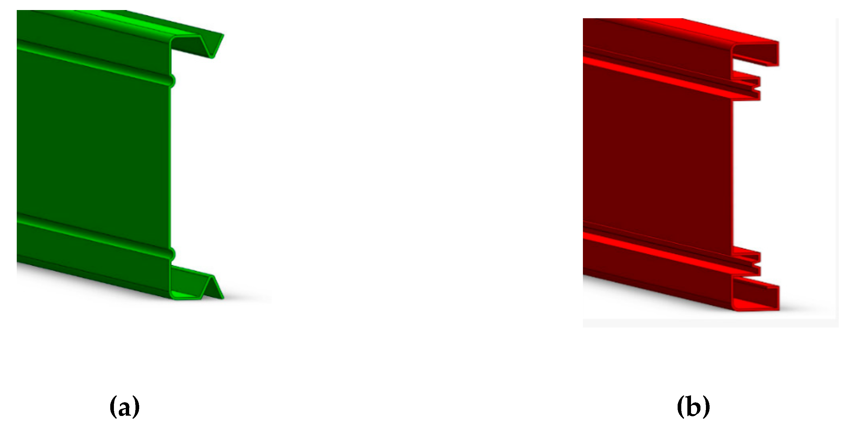
o C under blast load(Laím et al., 2015). The cross-section dimensions of stud under consideration in the present study are shown in
Table 3. The stiffness of section under blast loading is reduced when compared to that under static loads. In the context of bending strength of stud, the essential role was played by compression flange and web. Two shapes of stud are shown in
Figure 3.
Interaction properties used in Finite Element Analysis
In current finite element analysis, the interaction between one element and other element plays an energetic role. The bond between experimental and analytical model depends upon the contact controls. It gives the accurate behavior of the structure. Initially, interaction property 1 was taken as general contact with tangential behavior. The blast pressure was given in the form of spherical air wave, therefore the interaction property 2 was taken as incident wave. The details of Interaction 2 are given in the
Table 4. Surface to surface contact between connections was used. Kinematic contact method and sliding formulation were used. In the experimental program, the stud wall related to a reaction frame using bolted connection was considered. Self-tapping screws M6, M10 were used to fix the connection in the present model.
The self-drilling screw connections were modelled as surface-to-surface connection. The connection between shank and plate were modelled as node to surface with some tolerance value.
Load application
Load was applied in terms of pressure. The scaled distance was determined using scaling law and the distance is 1.575 m/kg
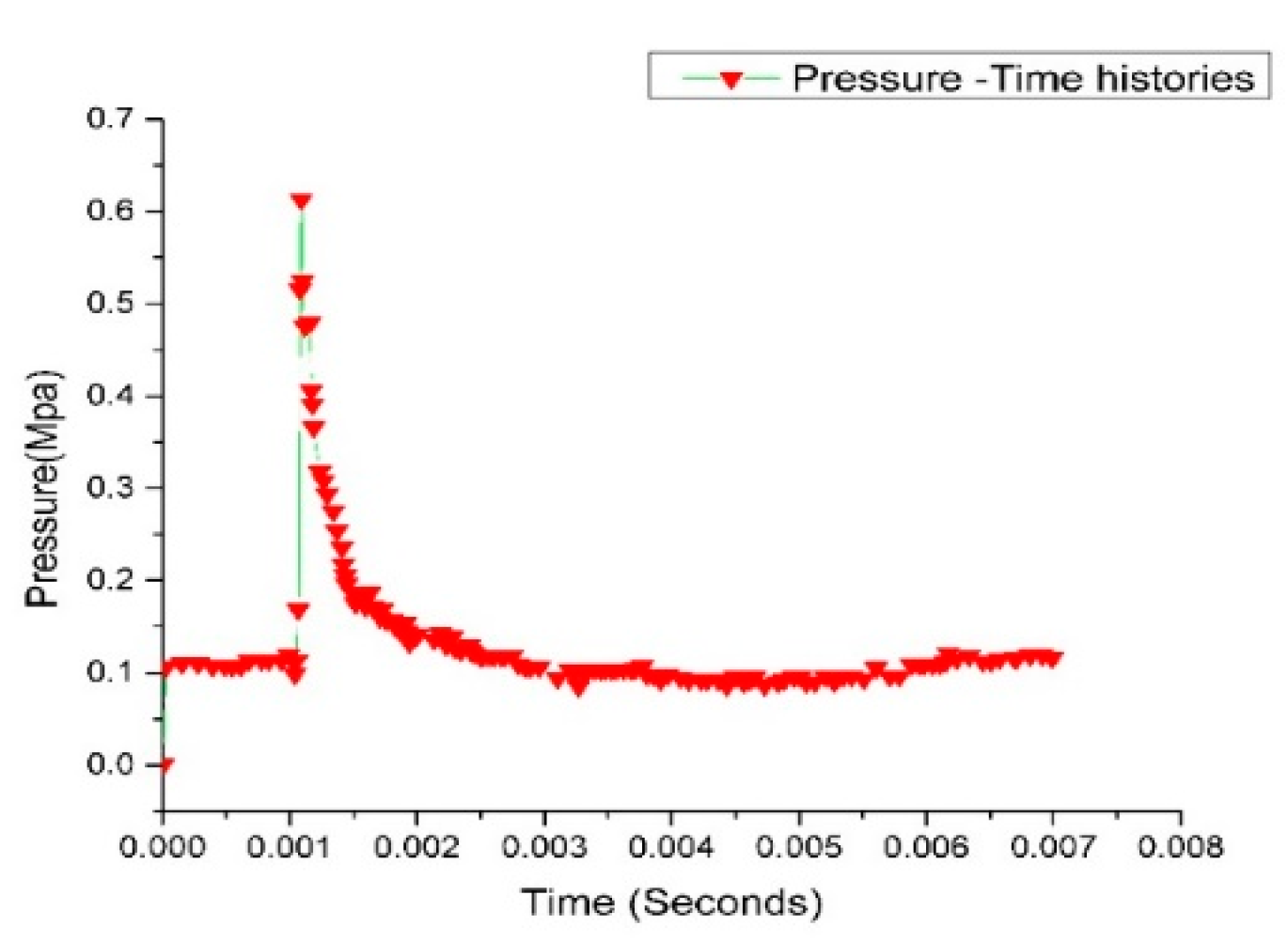
1/3. During blast, pressure was captured using pressure transducers at four locations in the stud wall. By using this data, frequency versus time was given as amplitude in modelling. Pressure was analyzed (shown in
Figure 4). Pressure versus Time curve was plotted. Conventional weapon Program (CONWEP) was used. As per the building design for homeland security, the equivalent pressure occurs at scaled distance which is equal to distance divided by the net explosive weight of TNT equivalent with whole power of (1/3).
Finite- Element Modelling- Explicit
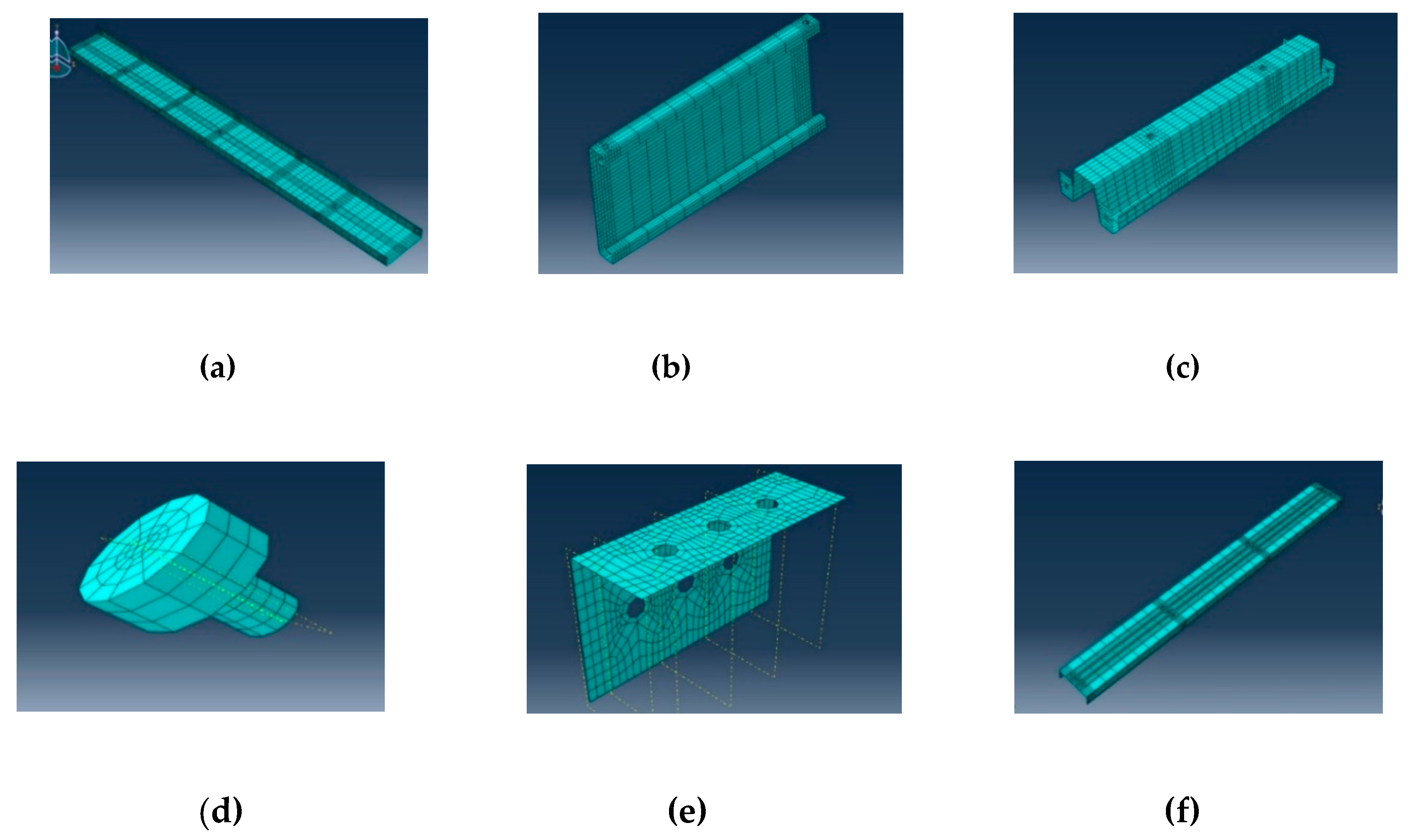
A structure subjected to high impact can be modelled using static resistance function which is essential to predict the structural response of wall under blast loads. Blast loaded structure can be analyzed using equation of motion to predict the response of the structure (J.M. Biggs, 1964). Cold-formed steel elements were modelled as shell elements. The sheathing material was also modelled as shell element. The solid rod and bolt were modelled as solid section with C3D8R. For washer split regions structured mesh were used. Mesh type depends upon the geometry of specimen as shown in
Figure 5.
Blast load
The orientation of explosive was considered at 1.565 m from mid height center of stud wall. Ammonium nitrate based packed emulsion explosive were used. In computational modelling, the explosive was placed which is perpendicular to X direction at the specified standoff distance as shown in
Figure 6(a). The response of stud wall was observed in various location as given in
Figure 6(b).
The predicted pressure from experiment was used in FEA. According to the experimental program, the results were captured up to 300 milliseconds. It was observed that within 7 to 10 milliseconds, the positive pressure wave hit and crossed the structure. It means that positive phase pressure occurs in between that time period. The maximum peak pressure occurred between 1 -1.5 milliseconds. The stud wall observed the maximum pressure and tried to spread the damage at various locations of the stud wall.
Validation using Experimental research by Whelan et al., 2016
Whelan et al. (2016) investigated cold-formed steel stud walls experimentally. As per the research, the out of plane deflection of the stud wall at the mid height was captured. In this investigation, an explosion in the open air was conducted on a stud wall. Three identical cold-formed steel stud wall specimens with dimensions of 2.440 m height and 1.220 m width were evaluated. Two tracks and four studs serve as the vertical and horizontal components, respectively. A buckle bridge system was installed in the middle of the wall to strengthen the wall's resistance to buckling when subjected to blast. The deflection at peak pressure was observed as 78 mm as shown in
Figure 7.
Artificial Neural Network (ANN)
Some laborious experiments in field of civil engineering cannot be carried out in the field. Numerical simulation study acts as a back bone support for those circumstances. In addition, ANN acts as a filler between experiment and numerical study. The performance, validation and error can be identified using ANN. Artificial learning is one of the advanced mathematical models used in various domains. The neurons in the human body are very influential. The communication of signals from human brain to internal organs through central nervous system is highly rapid. The mimics of human neural network is resembled as Artificial Neural Network (ANN). The processing units involves three major division such as input layer, hidden layer and output layer. Data from input layer and output layer is processed by the hidden layers. It is the important layer for non-linear data. The number of hidden layers depends on data complexity with trial-and-error process. There is strong connection with one layer data with another layer. The weight of each data can be measured and associated with data in another layers. The objective of network training is to maintain the data which gives less percentage of error and improve the performance of model (Huang et al., 2021). The construction between input and hidden neurons through weightage and biases(Armaghani et al., 2017) .The given data should be trained, matrix should be in architecture and finally the neurons giving better performance. The input and output data should be scaled within the suitable range gives the suitable function. In the data training unit, Levenberg Marquardt learning algorithm is one of the best and highly accuracy method(Dogan et al., 2017) . The advantage of ANN is to fit the input data and output data with minimum number of errors. The data was arranged in a form of matrix. The training data is the essential step for the prediction of model in ANN. The resilience analysis after explosion was carried out in ANN (Zuruda J.M, 1992). The damage scale was analysed using ANN approach. Post explosion study were carried out on the structure and off the structure. In the machine learning models, four target level of damage such as damage scale, recovery decision, recovery time were analysed. To get the maximum performance the model was analysed four times. The importance of input variables was explored by chi square test (Dai et al., 2016). Vibration analysis and damage detection was carried out in the steel beams and frames. The damage indices are computed using the mode shape components and their resultants to improve the precision and effectiveness of damage identification. The MSEDI-based ANNs predicted the damage magnitudes of the single and multiple damage scenarios with errors of up to 0.95% and 1.12%, respectively(Nick et al., 2023). Steel column bucking resistance was examined using finite element analysis and validated using an artificial neural network. To generate useful metaheuristic-trained Artificial Neural Networks for predicting the ultimate buckling stress of High Strength Steel columns. It confirmed that the broad usage of metaheuristics as training algorithms has a considerable impact on ANN model performance. A greater level of accuracy was achieved, with coefficients of determination above 0.998, demonstrating machine learning as a feasible solution technique for this highly nonlinear problem(Kaveh et al., 2023) .By minimising the number of rejects, the efficiency of the finishing process for low-alloyed seamless steel pipes was improved. The artificial neural network (ANN) was used to inspect the dimension of pipes with unknown shape. The temperatures at Measuring Points 2 (T2) and 3 (T3) were defined as the target variables for the ANN model. A mean temperature along the pipe is expected for these temperatures. According to the employed steel alloy and the specified grade, the forecast shows whether the temperature limit is met. These forecasts are useful because they enable operators to produce a wide range of varied pipe dimensions without rejections or energy waste.(Langbauer et al., 2022). An artificial neural network (ANN) model for thermal shrinkage of seamless steel pipes. The creation of a novel ANN model that predicts the cold diameter of seamless steel pipes using a more sensitive target variable. ANN models were validated because they provide more information about model behaviour than a single statistical measure (e.g. MSE, R2).(Langbauer et al., 2023). A feed-forward neural network was built to determine the fatigue life of pearlitic Grade 900A steel based on the number of cycles of the given stress level in the load block, occurrence ratio, and overload ratio. .Additionally, the developed ANN can forecast the material's fatigue life for all conceivable values inside the training range right away(Masoudi Nejad et al., 2022).
Time-Displacement
The time displacement of stud wall was analysed using finite element model. According to the earlier discussion, displacement in four different locations was captured. The data from finite element analysis was verified using mathematical model (ANN). In this current study, totally 12 input parameters, hidden layers and one output was validated for each FE model as shown in
Figure 8. In the model F26-RWC-M156-1.19, the data should be fall along the output line of neural network. It was observed that the finite element data ties clearly, which provides the optimum outcomes.
Response Surface Methodology (RSM)
RSM is an advanced quantitative parameter tool. It is used for data optimisation and prediction. The inputs and outputs were set up similarly to a FEA model. The unit's system was also similar to the FEA model. Surface plots in Minitab are used to relate the two predictor variables to the response variable in a regression model. The plots, which depict the predicted response surface as a three-dimensional surface, can be used to identify patterns and trends in the data. The absence of any connection between the two predictor factors and the response variable may be implied by a flat surface. A nonlinear relationship between the two predictors and the response variable may be indicated by the curved response surface. In Minitab, the coefficient estimates, standard errors, p-values, and R-squared value are used to interpret the results of polynomial quadratic regression analysis. It is necessary to carefully examine these results in order to determine whether the model provides a good fit to the data. Moreover, to assess the significance of the predictor variable(s) effects on the response variable. The RSM model properly predicted the concrete's properties (R2=0.99). The engineering properties of mortar have also been experimentally and statistically examined. RSM and ANN are two important methods for displaying and assessing such correlations for validation purposes (Kavya, 2022)
Time- Displacements History
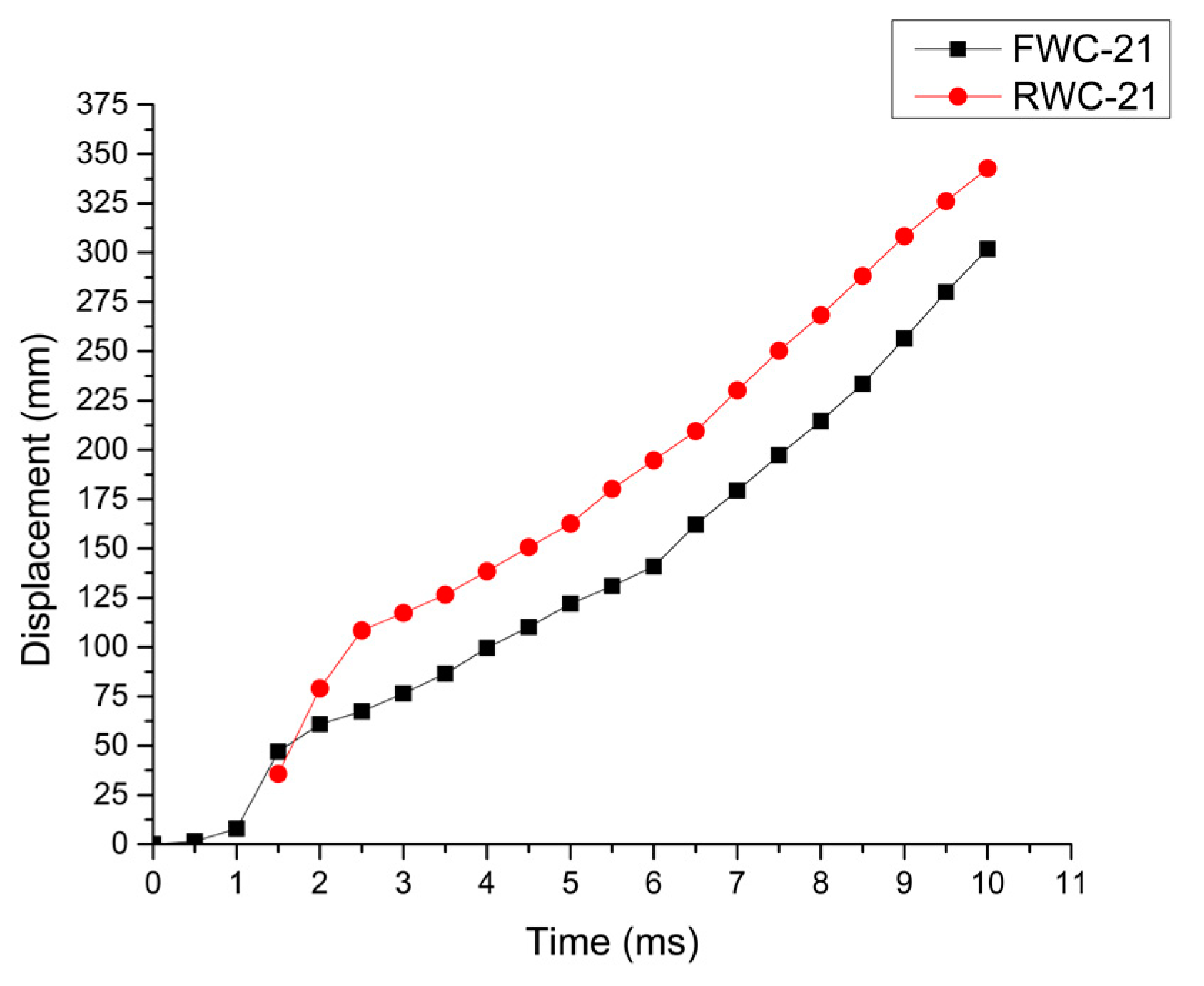
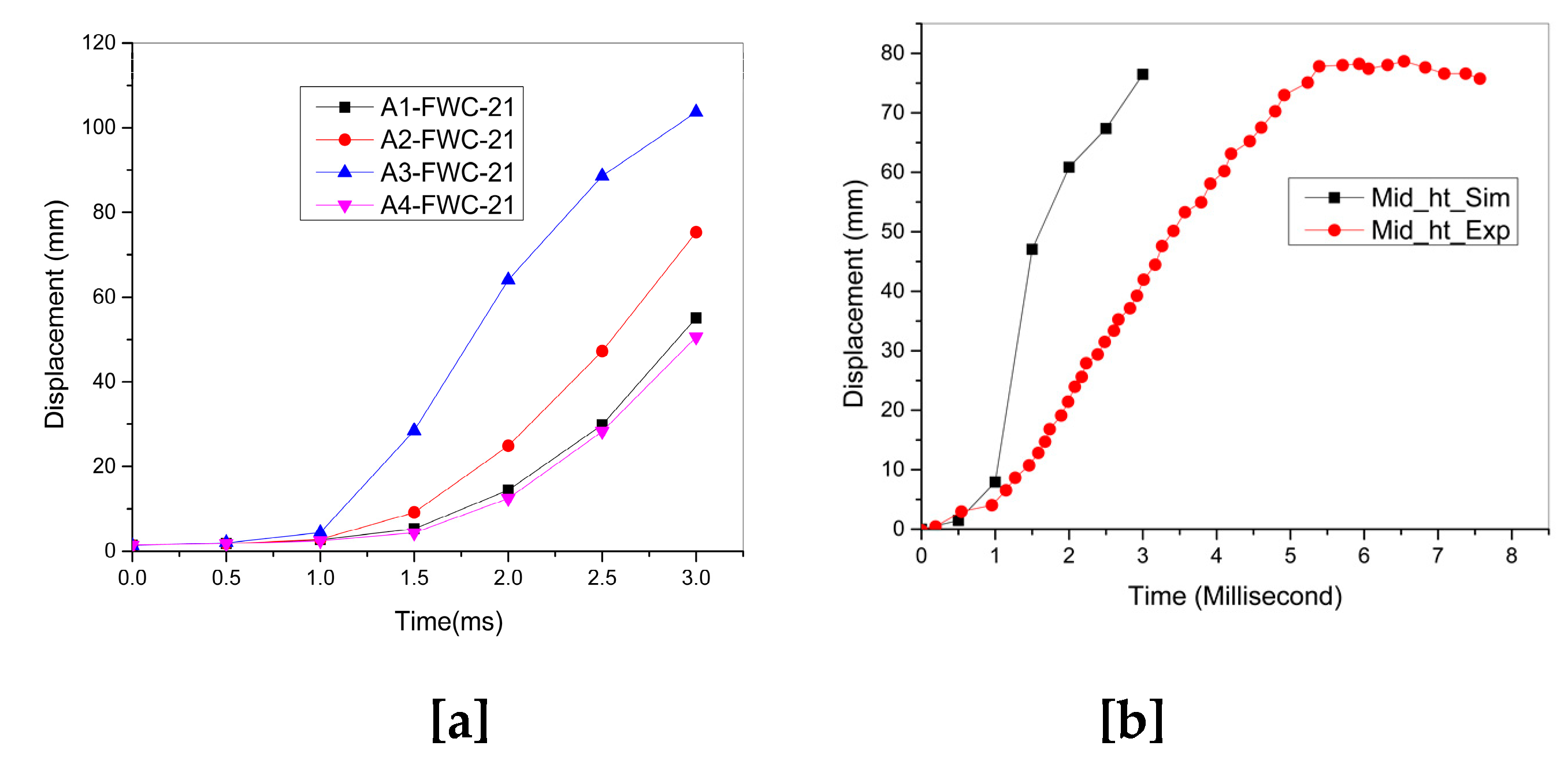
Four different specimens were used in the current research. All the models were analyzed individually and the results are captured as shown in
Figure 9. It was observed that F26-RWC-M156 subjected to high deformation when compared to other models.
FWC-21-M156
In this stud model, flange corrugation and web corrugation were provided at certain locations. Normally fillet portion can easily transfer shear stress. Two numbers of web corrugations were given. Flange is the most preferable portion to with stand the bending moment in the section. In account of this, corrugations were introduced to take more deformation and energy absorption. The maximum deformation at the mid height of the specimen was captured as 76 mm at the step time of 3 millisecond, when compared to the experimental data (Whelan et al.), which was 78 mm. Therefore, experimental and modelling data was overlapping each other. The physics of simulation resembles like experimental model. The time versus displacement of FWC-21-M156 as shown in
Figure 9 (a) and (b). The deviation of FEM and experiment is 2.6% as shown in
Figure 9 (b).
In the location A1-203 mm from the bottom of the wall, the deformation captured was 55 mm at the step time 3 millisecond, in comparison with experimental data, which was 51mm. The percentage of deformation in the stud was increased by 7.8. The time-displacement history of this specimen is shown in
Figure 9 (b).
In the second spot A2, the deformation in the simulation was captured as 75 mm at the step time of 2 milliseconds. In experiment, the same location data was extracted as 58 mm. The percentage of deformation in the stud was drastically increased by 29. In the third spot A3, from the simulation, the deformation value of stud was 103 mm. Whelan et al. experimental investigation, the extracted data was 54mm. The percentage of deformation increased tremendously by 90.7. Excessive deformation developed due to geometry of stud wall and web crippling of stud. It was observed that the energy dissipation is very good by creating new mechanism in stud wall. The stud tries to form a greater number of plastic hinges. The final spot of stud is A4, which is nearer to the top track. At this zone, which is slightly far away from the surface, the deformation was 16 mm in the experiment and 50 mm in the simulation. Therefore, the percentage increase of deformation is 212.5
F26-RWC-M156
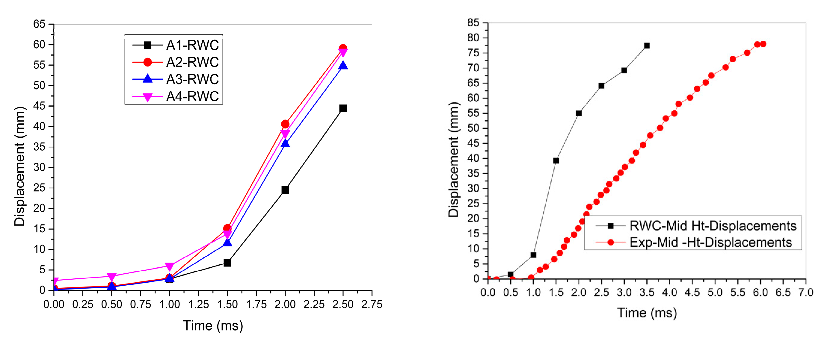
In this model, web corrugations were created in rectangular manner. The main objective of the creation of this model is to delay the pressure timing inside the stud wall. When a car subjected to any impact, the driver head is going to hit on the steering of the car immediately. At this scenario, the air bag opened and reduce the time of hitting which causes less impact on driver head. Likewise in this model, flanges surface directly in contact with pressure. This pressure will transfer from flange to flange through the mediator web, if the energy will be delayed by introducing this corrugation in the web portion.
In the location A1-203 mm from the bottom of the wall, the deformation captured was 44 mm at the step time 2.5 millisecond, in comparison with experimental data [Whelan et al], which was 51mm. The percentage of deformation in the stud was decreased by 13.7, because of introducing excess web area. It was concluded that the web corrugation reduces the permanent deformation of stud wall. In A2, the deformation in the simulation was captured as 59 mm at the step time of 2.5 milliseconds, compared to 58 mm from experiment. The percentage of deformation increased by 1.7. There is a very good resistivity against the same pressure by web area (as shown in
Figure 10 (a) and (b)) It was concluded that, energy absorption is very good in this scenario.
At A3, from the simulation, the deformation value of stud was 54 mm. Whelan et al experimental investigation, the extracted data was 54mm from experiment. It was observed that the stiffness remains same by disturbing the web portion of section. At A4, which is nearer to the top track, which is slightly far away from the surface, the deformation was 16 mm in the simulation and 58 mm in the experiment. Therefore, the percentage increase of deformation is 34 mm.
Influence of stud thickness
The deflections are controlled by increasing the thickness of stud. Two different shapes of stud were modelled and analyzed. It was observed that, by reducing the width of flange in channel section, stiffness can be increased. The web portion of stud were subjected to ‘n’ number of perturbation. The thickness of stud was increased from 1.19 to 1.5 mm in FWC-21-M156, and F26-RWC-M156 model. The stud thickness was 1.3 times increased and deflection was decreased up to 0.9 times. Both models controlling the deformation in an efficient manner. Finally, it was observed all these two models have a good resistance against blast loading. The summary of results is shown in
Table 5.
FWC-21-M156-1.19
In this model FWC-21-M156-1.19, the data was fitted properly and analysed with almost zero error as shown in
Figure 11. It was concluded that there was good agreement between computational model and mathematical model.
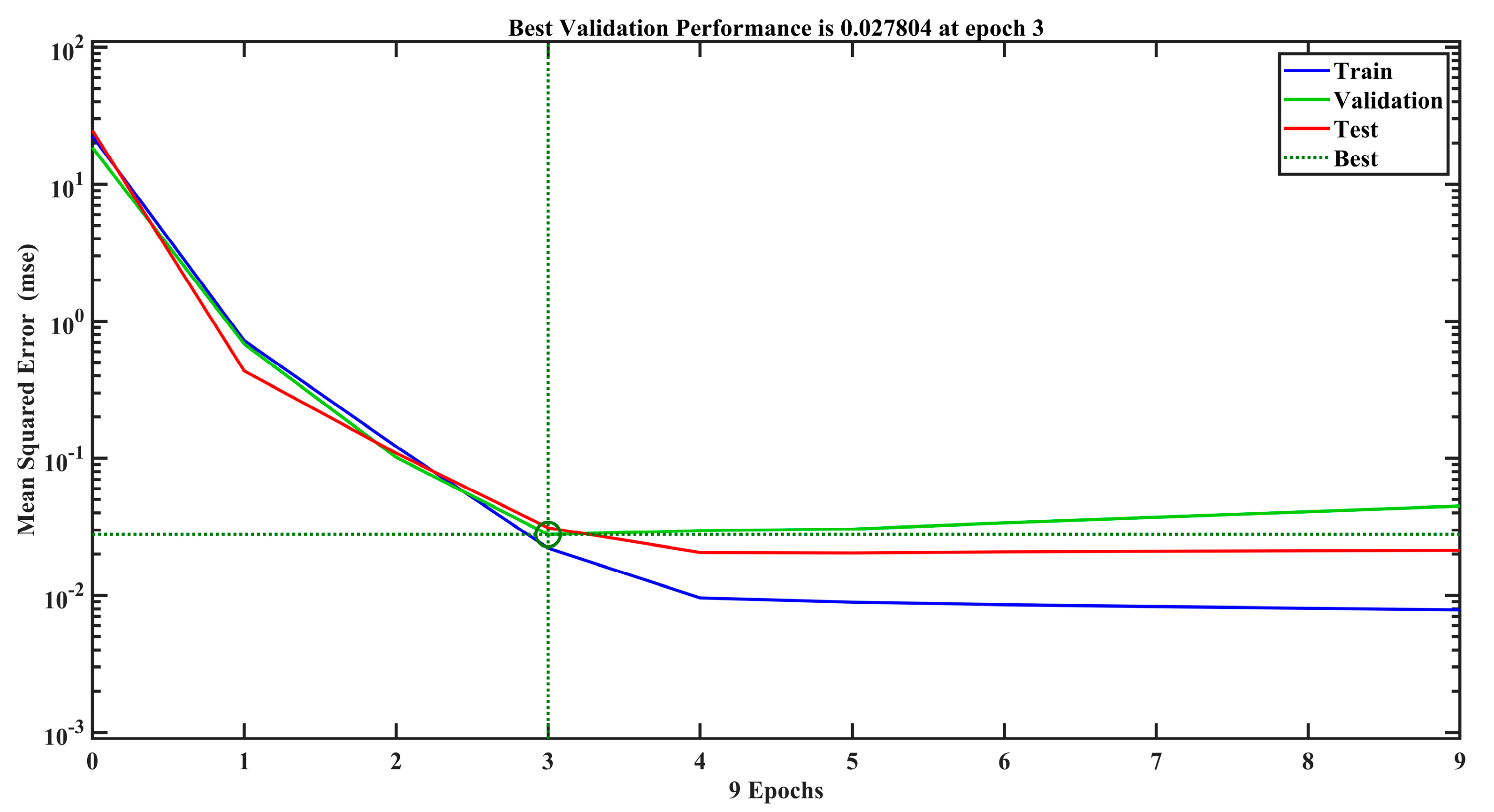
The mean squared error of FWC-21-M156-1.19 which has a deteriorated tendency as shown in
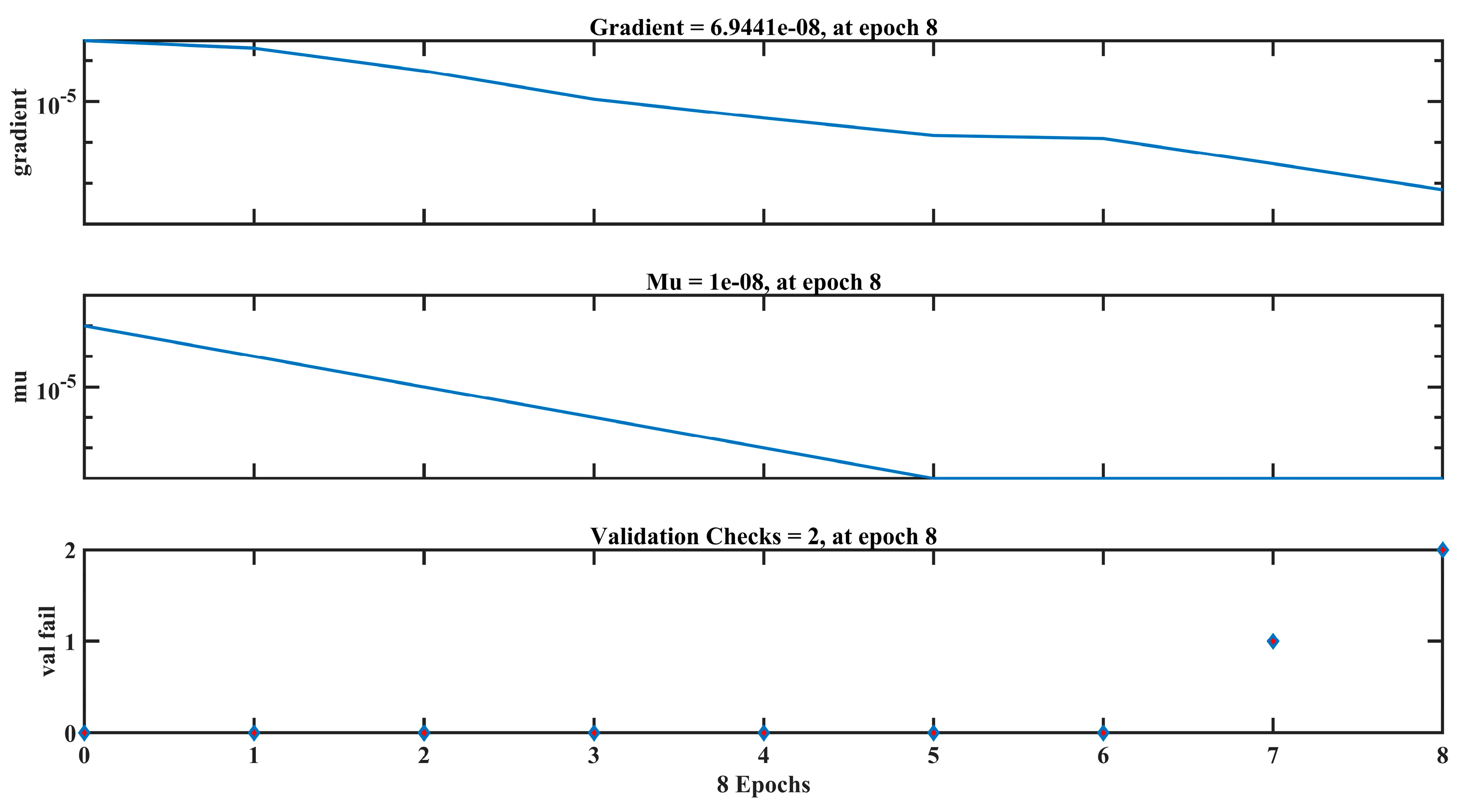
Figure 12. This pattern also recognized as a neural network success with epoch 3. There are three different lines plotted in the diagrams which indicates the input and output vectors has been arbitrarily divided in to three groups. Overfitting may delay if the training stopped as soon as the proposed performance on the training set is attained.
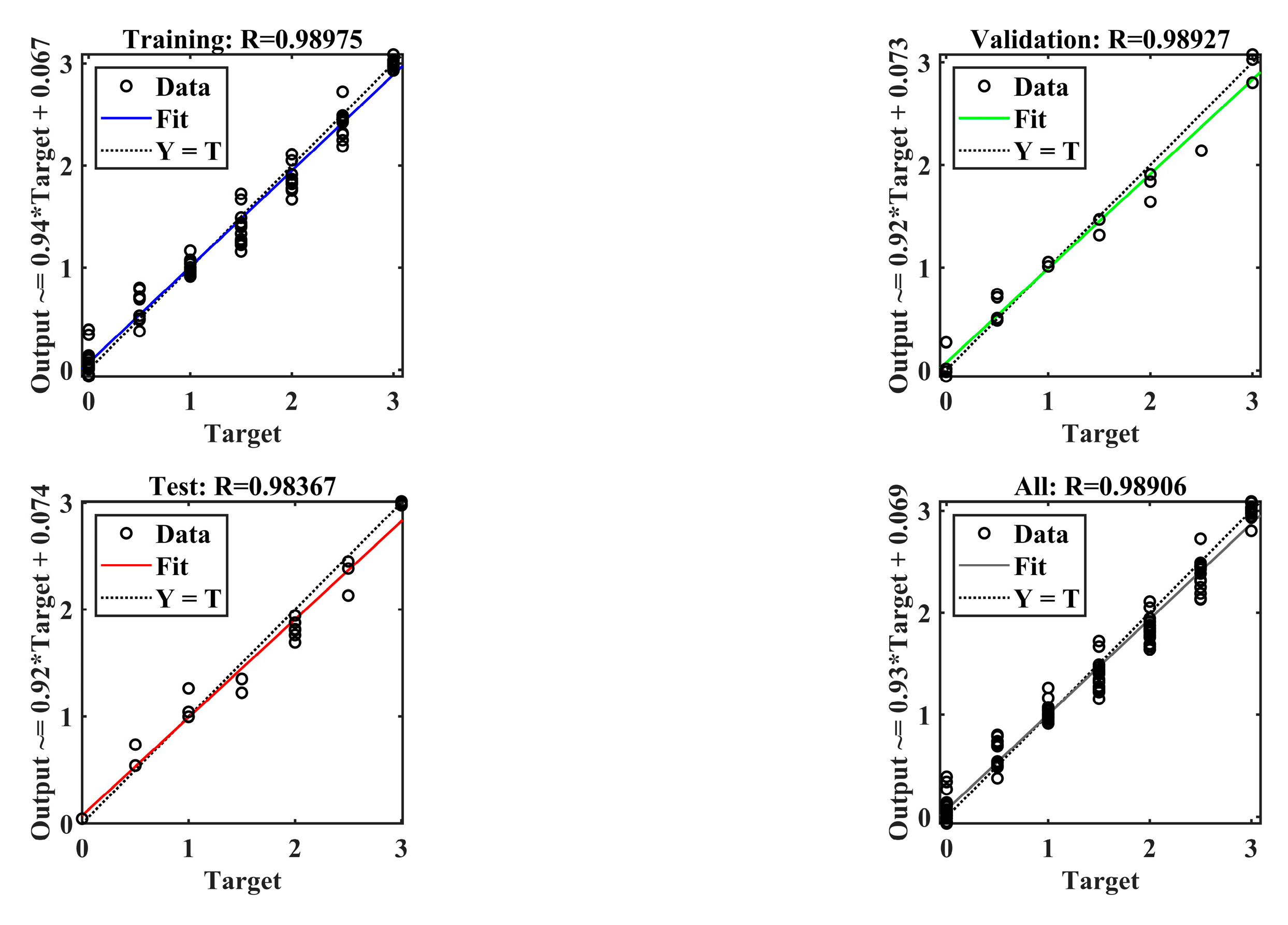
The regression plot of model FWC-21-M156-1.19 as shown in
Figure 13. The R values for the model recommended an ideal match throughout the entire data set with training values of 0.989, validation having value of 0.989, test having a value of 0.983, and all having a value of 0.9890 respectively.
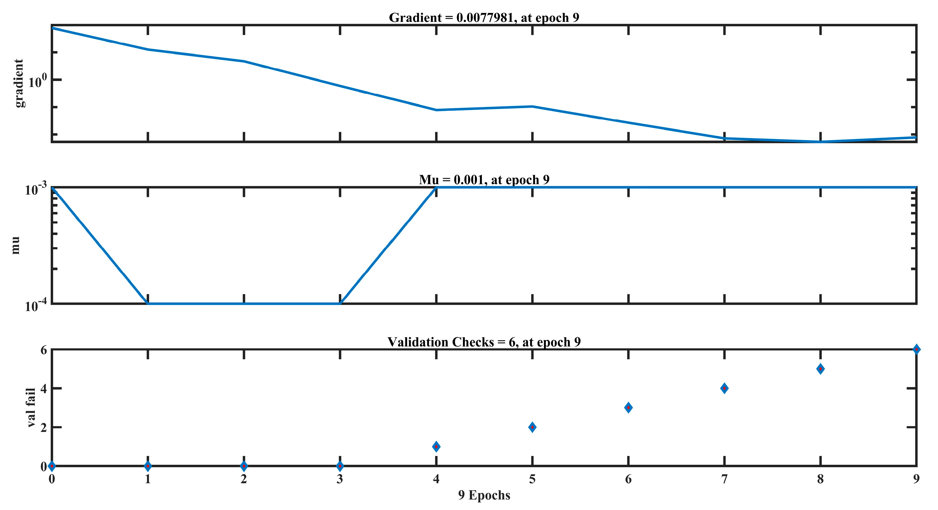
The fit plot of stud displacement was shown in
Figure 14. The stud displacement strengthens after 4 epochs, which closely agrees with the model.
F26-RWC-M156-1.19
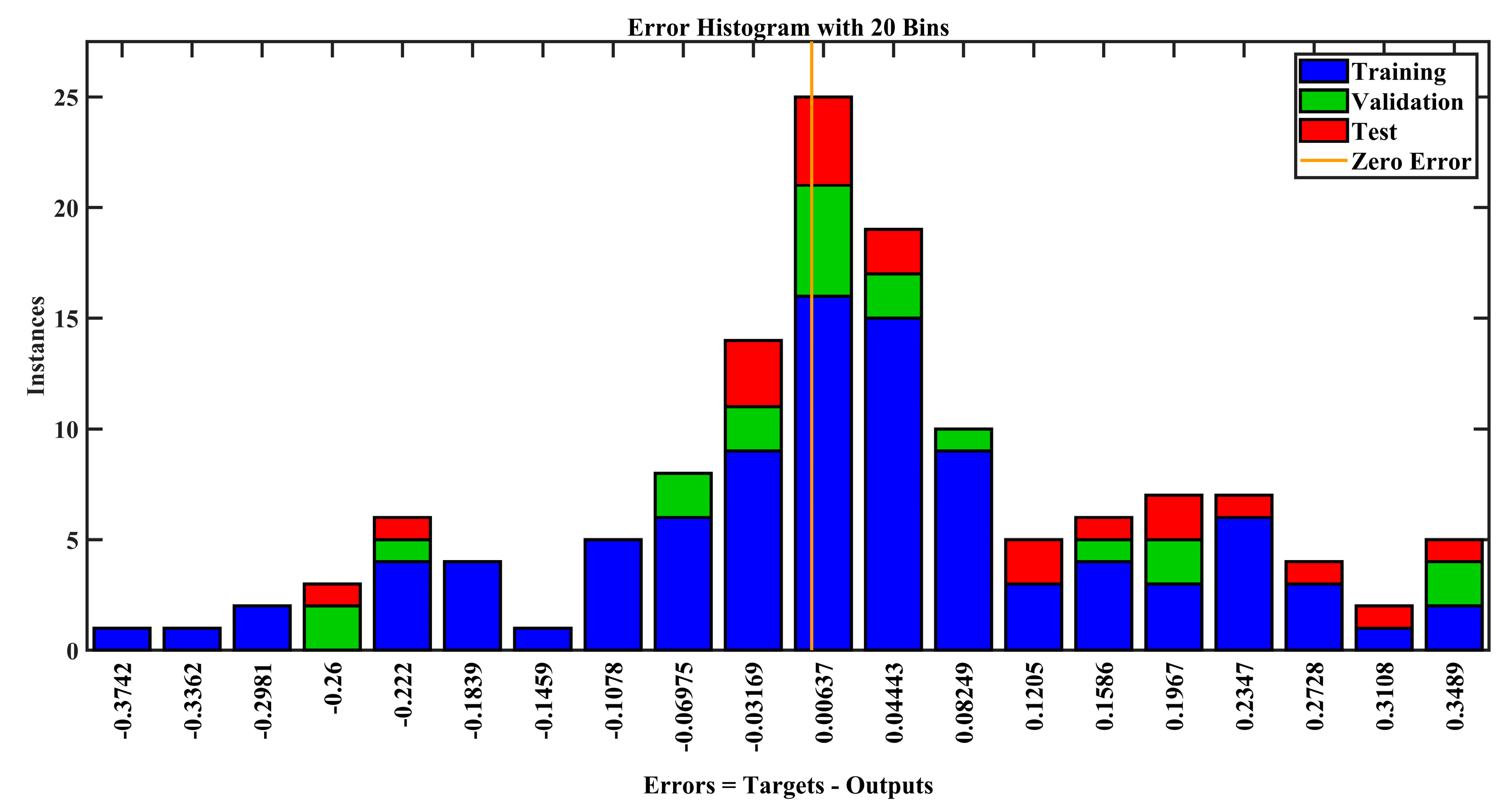
In this model F26-RWC-M156-1.19, the data was fitted properly and analysed with almost zero error as shown in
Figure 15. Out of 20 bins 16 were filled and data was spread in equal manner. It was concluded that there was good agreement between computational model and mathematical model.
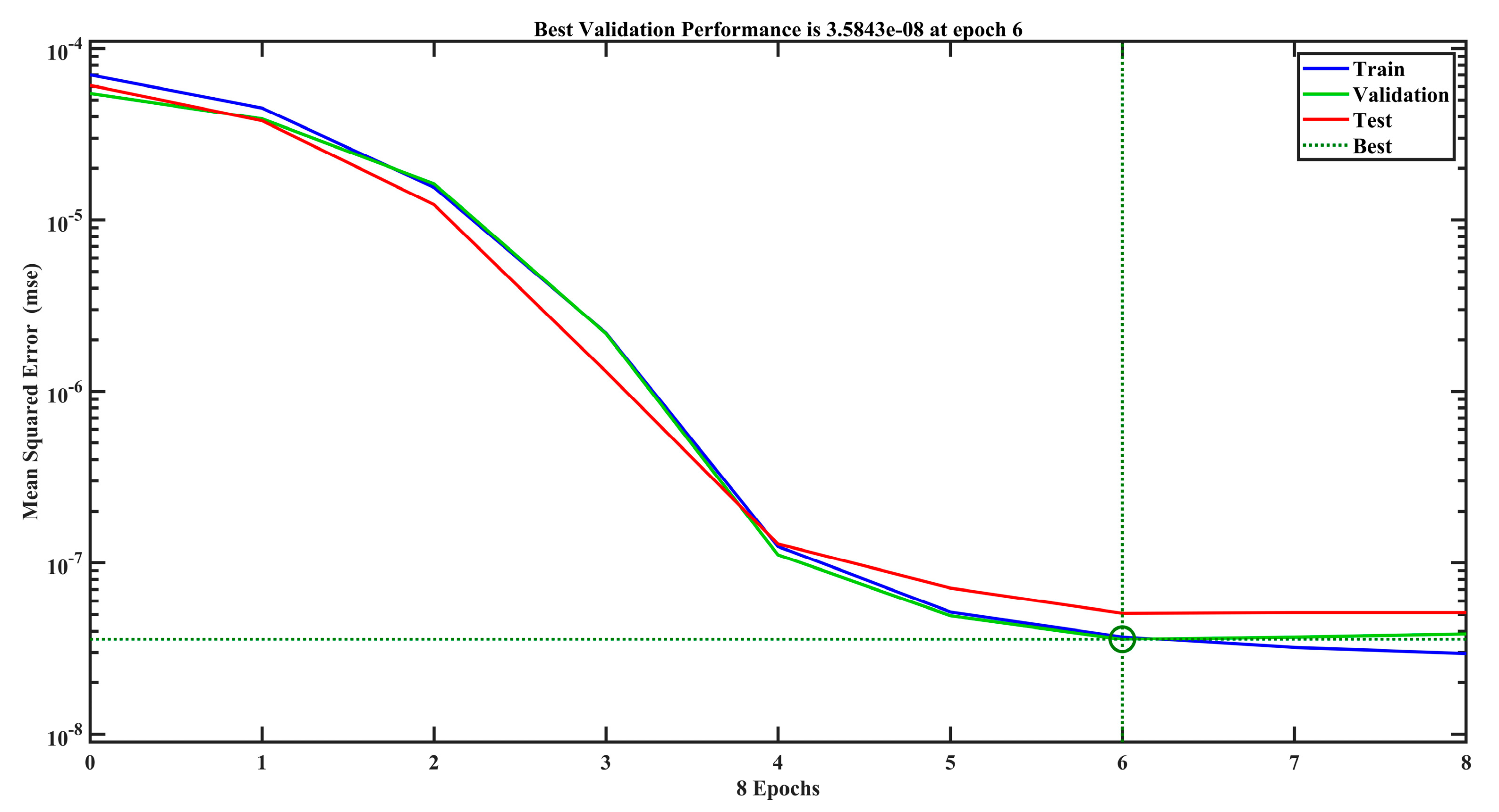
The mean squared error of F26-RWC-M156-1.19 which has a deteriorated tendency as shown in
Figure 16. This pattern also recognized as a neural network success with epoch 8.
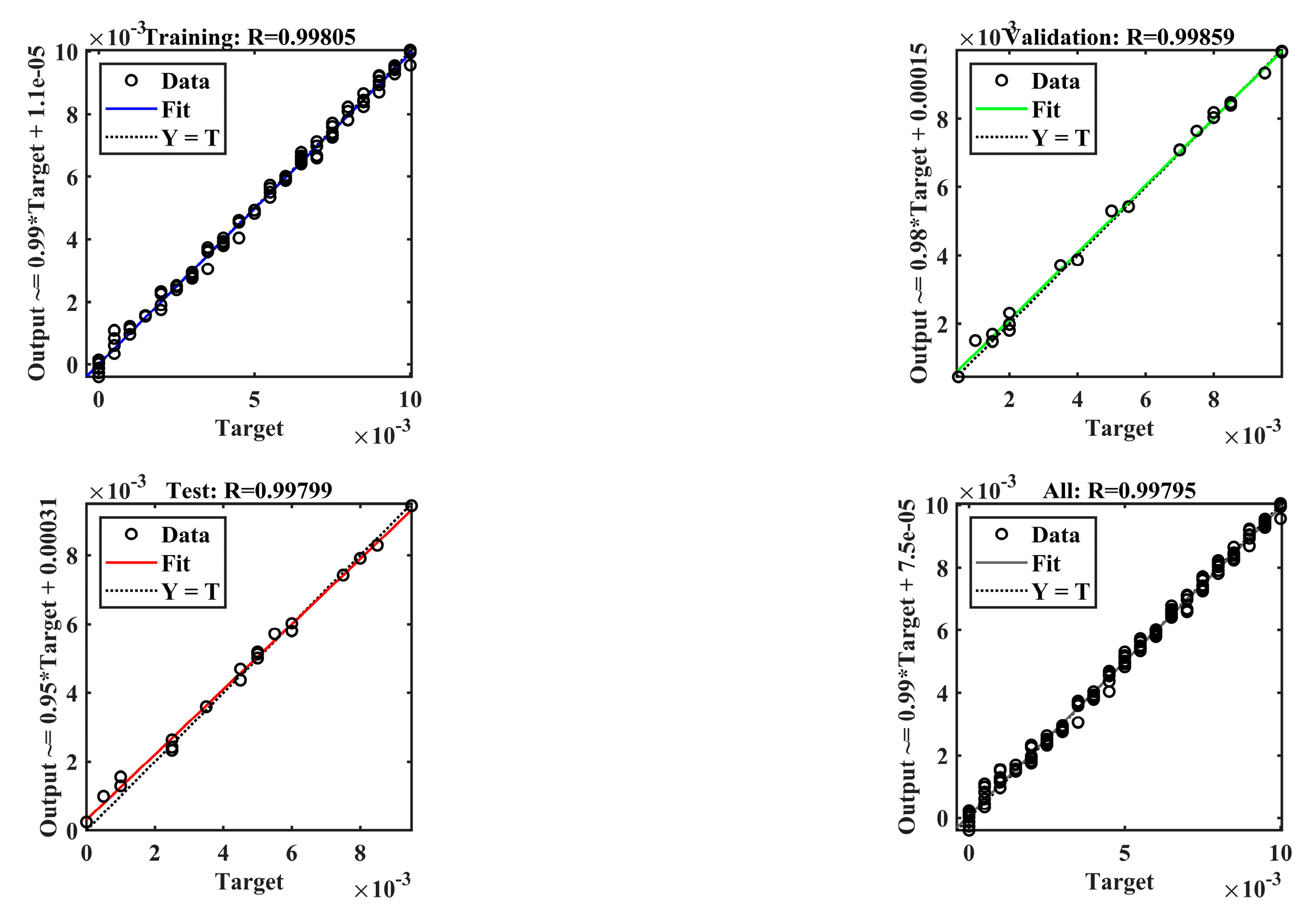
The regression plot of model F26-RWC-M156-1.19 as shown in
Figure 17. The R values for the model recommended an ideal match throughout the entire data set with training values of 0.9979, validation having value of 0.9985, test having a value of 0.998, and all having a value of 0.9976 respectively.
The fit plot of stud displacement was shown in
Figure 18. The stud displacement strengthens after 2 epochs, which closely agrees with the model.
Validation on RSM
Multiple linear regression is a statistical approach for modelling the connection between two or more independent variables and a dependent variable. In this study, time and pressure were the independent variable. Displacement was the dependent variable. The goodness of fit of the model can be evaluated using measurements such as the coefficient of determination (R-squared) and the analysis of variance (ANOVA) table, which provide information on the proportion of variance explained by the model and the overall statistical significance of the model. RSM design involves a combination of statistical approaches, experimental design principles, and mathematical modelling to determine optimal factor settings and improve process or system performance. It enables systematic investigation of the factor space and provides insights into variable relationships as shown in
Table 6.
FWC-21-M156-1.19
The flange web corrugation (FWC) with a mass of TNT as 1.56kg was investigated and validated by ANN and RSM. ANOVA analysis for the plots of displacement and time with significant results and values has been summarised in
Table 7 and
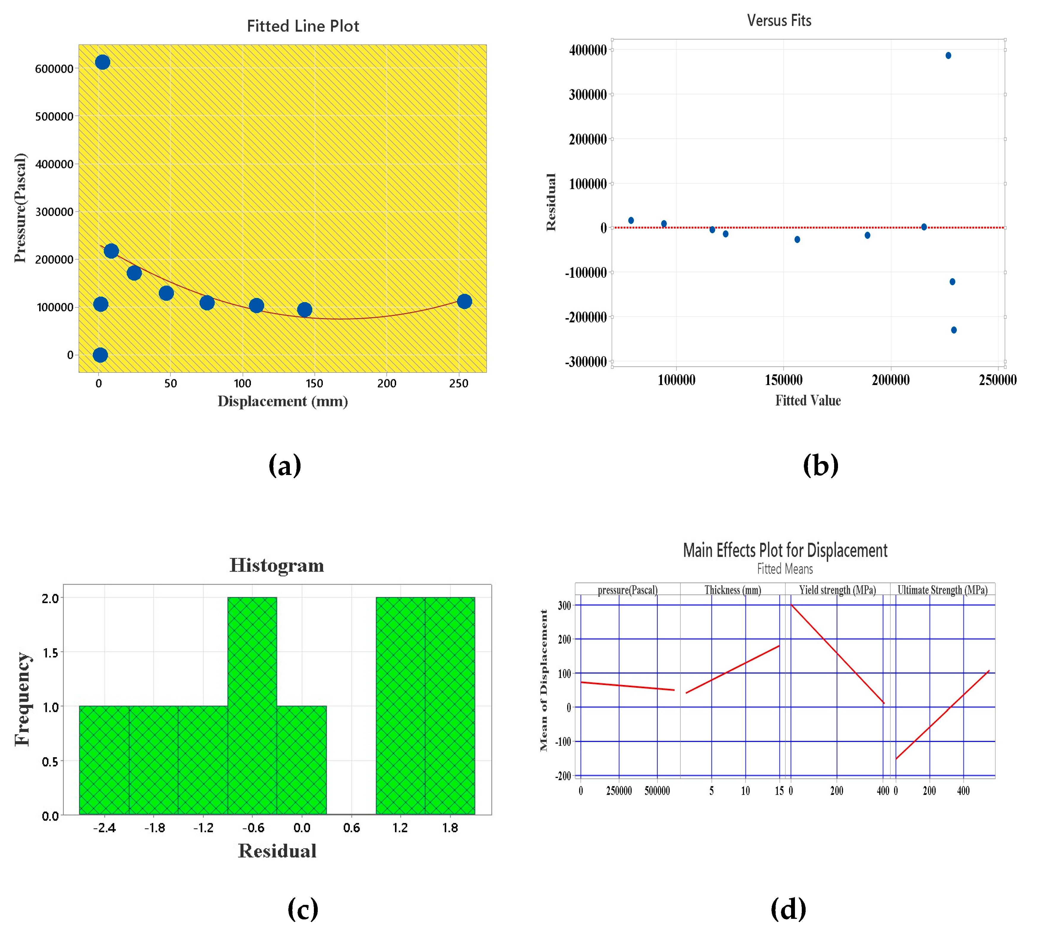
Table 9, respectively. An ANOVA or regression residual plot is a graphical representation of data that is used to examine the fit of a regression model. It is critical to evaluate the residual plots to determine whether the traditional least-squares assumptions have been confirmed or not.
The regression R
2 values more than 90%, then the basic least-squares regression produces reliable coefficient estimates with the smallest coefficient variance available. In this statistical model, the R2 values were reliable as shown in
Table 8.
The main effect graph is to examine the impact of each independent variable on the dependent variable while ignoring the effects of other factors. It enables to spot trends or patterns in data and see how the dependent variable changes when the independent variable changes. In this model, dependent variable was displacement. The pressure, thickness, yield strength and ultimate strength are the independent variables. The results were highly significant as shown in
Figure 19(d).
Regression Equation
The mathematical relationship between the displacement and pressure, thickness and time variables in a regression model is represented by a regression equation. Based on the values of the pressure, thickness and time, the equation is used to estimate or predict the value of the displacement.
The relationship between pressure and displacement has been proven to be highly significant using polynomial regression. as shown in
Figure 19(a)
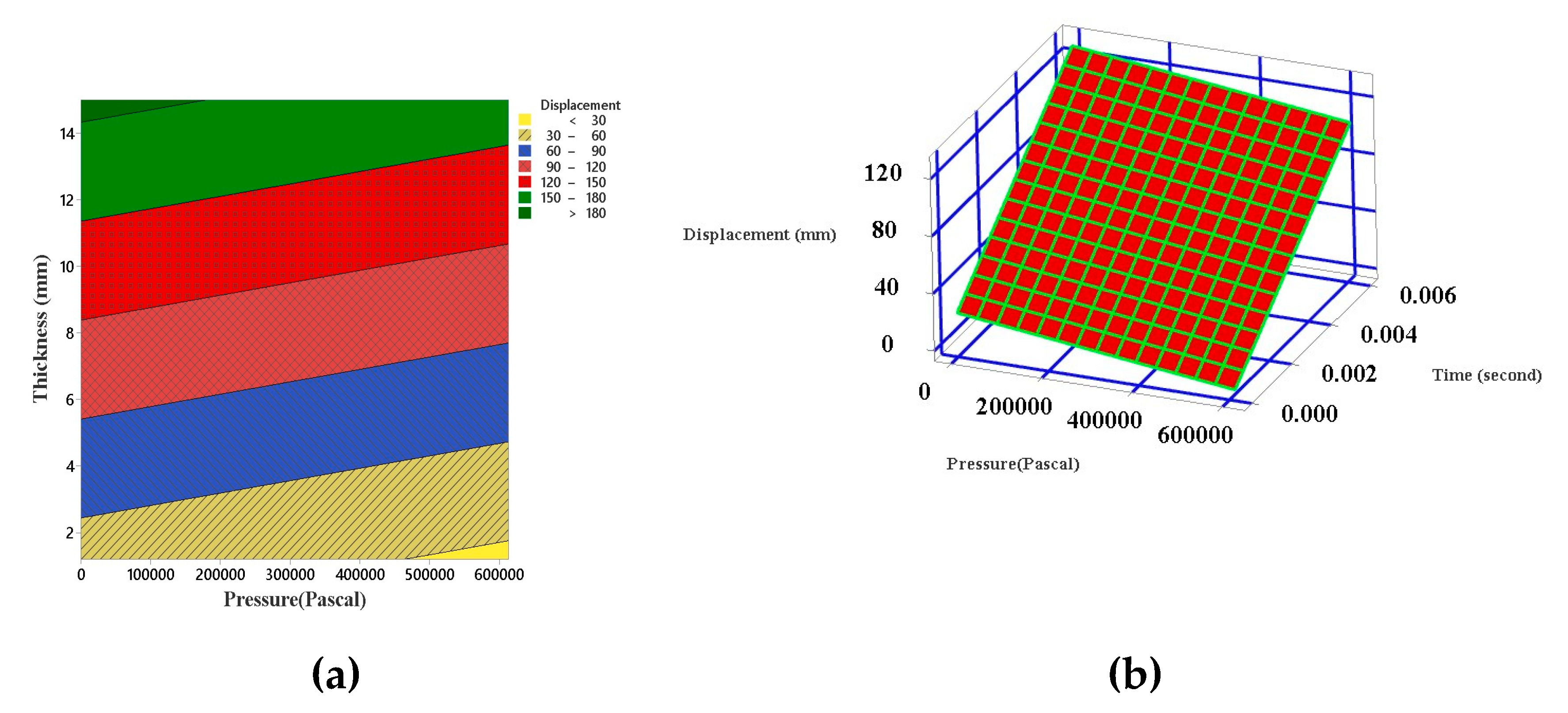
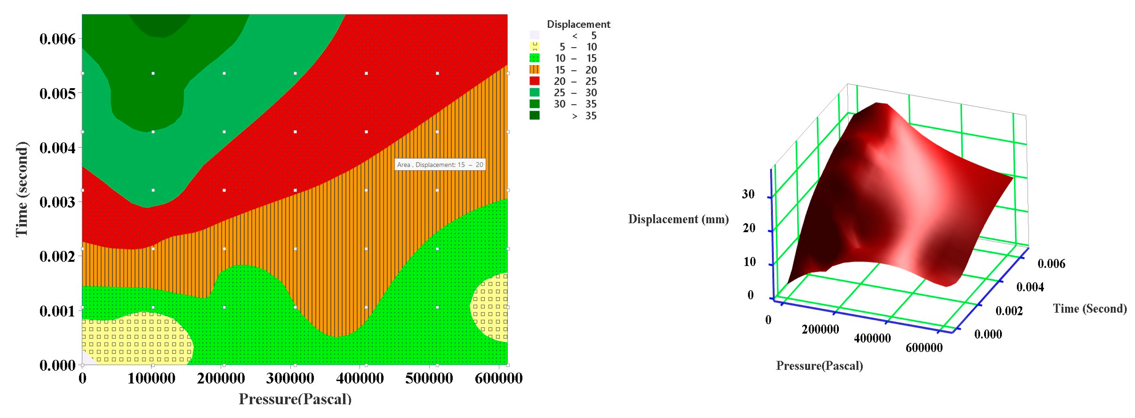
The surface plot of displacement, time and pressure shows a flat surface. 0It indicates a linear relationship between parameters. The displacement of stud was increased due to increasing time as shown in
Figure 20 (b). As a result, displacement is directly proportional to time. It was concluded that introducing new elements that can dissipate energy and control the displacement was one of the good ideas. When an explosion occurs, a large positive pressure wave strikes the wall, increasing displacement relative to pressure. The contour plot of pressure versus thickness was shown in
Figure 20(a). The maximum pressure can be exerted by the sheathing material of thickness 14mm.The displacement was observed more than 180 mm.
F26-RWC-M156
The Rectangular web corrugation (RWC) with a mass of TNT as 1.56kg was investigated and validated by ANN and RSM. ANOVA analysis for the plots of displacement with significant results and values has been summarised in
Table 9.
Analysis of Variance for Displacement
Regression residual plots, also known as ANOVA plots, are graphs of data used to assess how well a regression model fits the data.
Table 9.
Analysis of Variance for Displacement.
Table 9.
Analysis of Variance for Displacement.
| Source |
DF |
SS |
MS |
F value |
p value |
|
| Regression |
2 |
1144.99 |
572.494 |
200.23 |
0.002 |
Significant |
| Error |
7 |
20.01 |
2.859 |
|
|
|
| Total |
9 |
1165.00 |
|
|
|
|
The regression R
2 values more than 90%, then the basic least-squares regression produces reliable coefficient estimates with the smallest coefficient variance available. In this statistical model, the R2 values were reliable as shown in
Table 10.
Regression Equation
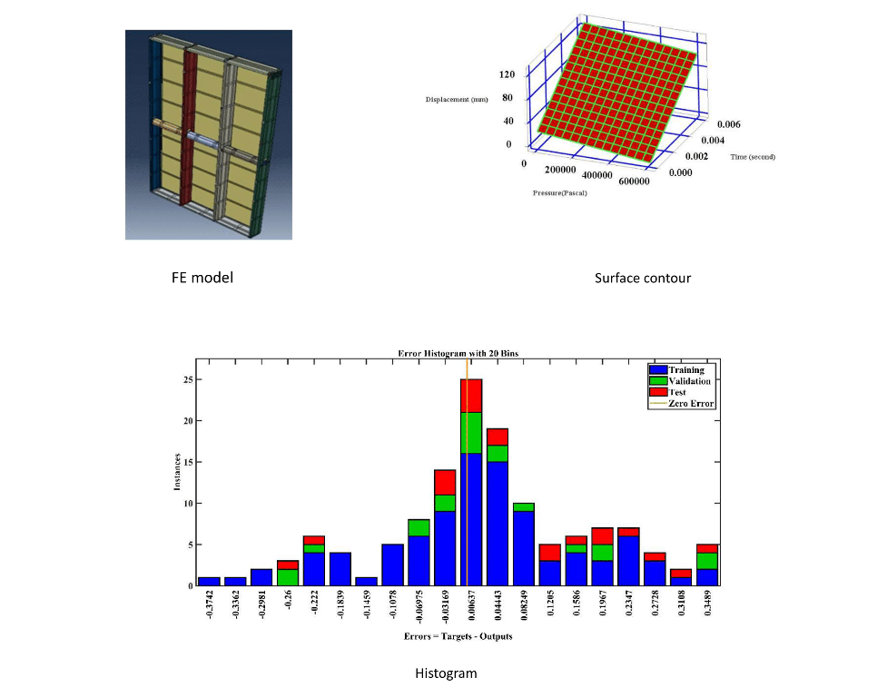
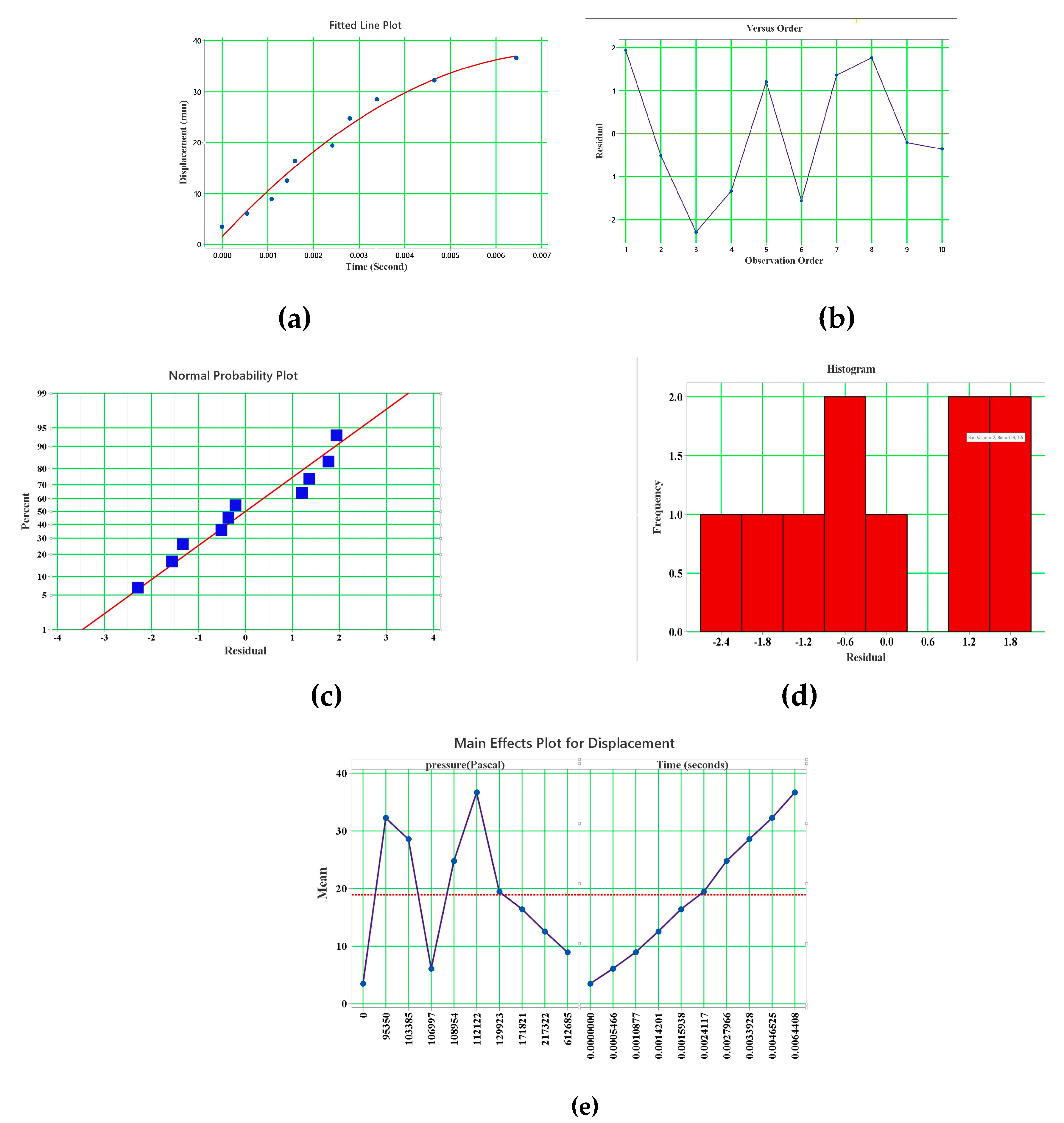
The mathematical relationship between the displacement (dependent) and time (independent variable) in a regression model is represented by a regression equation. Based on the values of the time, the equation is used to estimate or predict the value of the displacement. The distribution of numerical data is frequently represented by histograms, which make it possible to spot trends, core tendencies, and outliers. It was concluded that data is reliable, if positive error was observed in the analysis as shown in
Figure 21(d).
The surface plot of displacement, pressure and time shows a bowed surface. It indicates non-linear relationship between parameters. The displacement of stud was as shown in
Figure 22 (b). The variation of pressure with respect to time was investigated as shown in
Figure 22 (a).
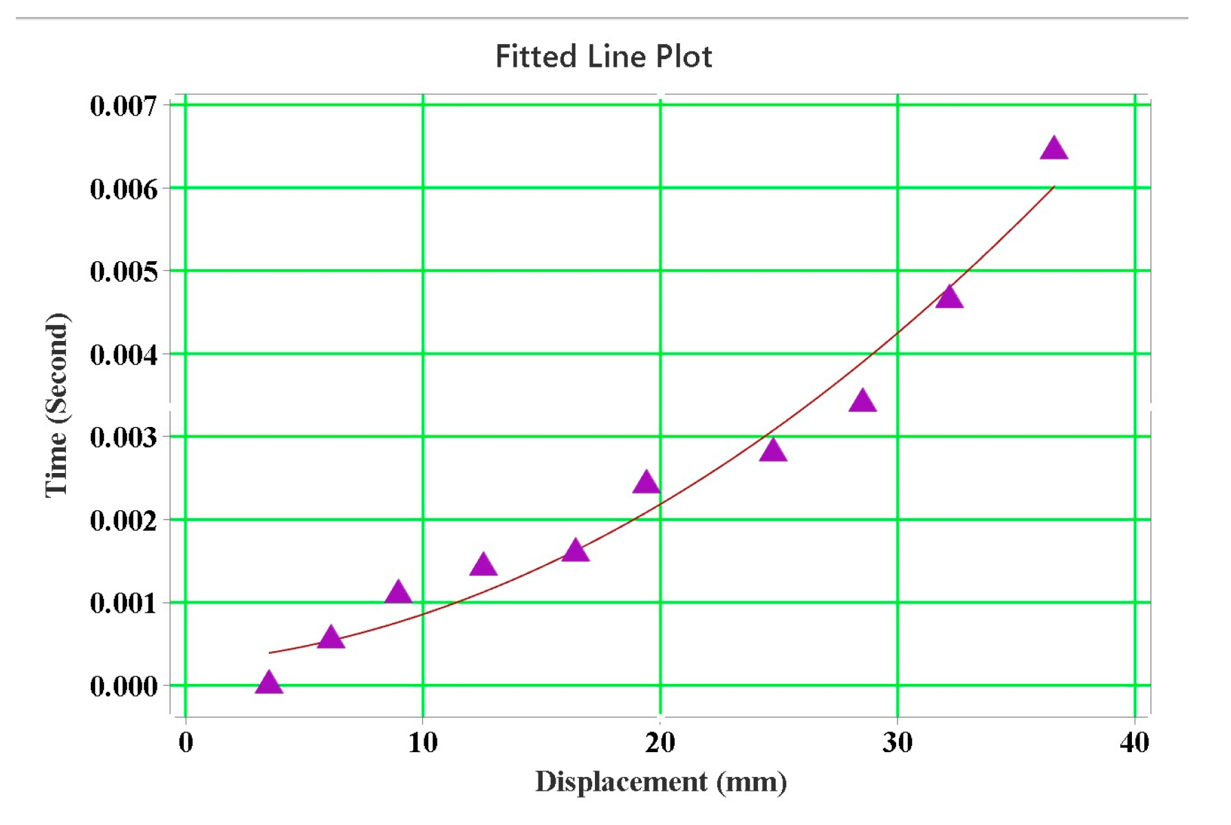
In the model, the regression analysis was carried out for time required to reach the maximum displacement. The fitted plot gives a significant result as shown in
Figure 23.
Regression Equation
The mathematical relationship between the displacement (dependent variable) and time (independent variable) in a regression model is represented by a regression equation. Based on the values of the displacement, the equation is used to estimate or predict the value of the time.
The basic least-squares regression gives accurate coefficient estimates with the minimal coefficient variance possible when the regression R
2 values are greater than 90%. In this statistical model, the R
2 values were reliable as shown in
Table 11.
Modes of failure
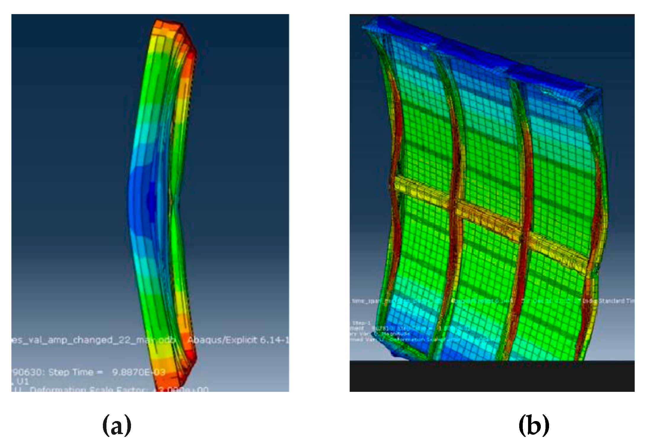
The FE simulation results are validated with experimental results referred from literature. There is a very good agreement between simulation and experimental results which shows the validity of the created models. After the detonation, the failed stud wall looks like the letter "C". Torsional buckling occurred on the exterior studs. Compression of web portion occurred in the interior studs. In this scenario, it is very important to create energy absorber in web portion to control deflection. Excessive element deformation occurred during analysis. In top and bottom track, tearing of bolt holes after blast was observed. At the mid span, studs were subjected to distortional buckling. The self-drilling screws were subjected to high yielding in the mid-height of the wall. These are the common failure modes occurred in all the models. Failure modes of model is shown in
Figure 19.
Conclusion
Web corrugated studs were analysed under blast loading. All the models were showing efficient result regarding resistance against blast. These models were found to be suitable for moderate blast.
In finite element analysis, model F26-RWC-1.5 found to have good control for deflection compared to the experimental model as shown in
Table 5. The premature failure can be resisted by self-tapping with some extent. The strength of screws should be increased. The integrity of wall assembly was maintained by buckle bridge in lateral direction.
During blast load application, it observed more amount of energy from sheathing material and stud. The flexural capacity of the stud wall was enhanced by buckle bridge and solid rod. The mode of failure occurred in interior stud was web buckling.
The failure mode of exterior stud was found to be distortional buckling. The strengthening of connection was required between bottom track and stud.
The mathematical model shows a good agreement between numerical model in aspects of error histogram, regression, training and best validation plots. In model F26-RWC-M156-1.19, the data was fitted properly and analysed with almost zero errors.
When the regression coefficient is more than 0.9, it shows that there is a strong positive correlation between the displacement of stud and the input variable in the regression model.
Regression equation gives an improved idea for prediction of displacement.
Author Contributions
SAV: conceptualization, methodology, software, investigation, validation, formal analysis, writing and editing the draft. NU: conceptualization, supervision, investigation, validation, editing and review the draft.
Funding
This research received no external funding.
Conflicts of Interest
The authors declare no conflict of interest.
References
- Armaghani, D. J., Mohamad, E. T., Narayanasamy, M. S., Narita, N., & Yagiz, S. (2017). Development of hybrid intelligent models for predicting TBM penetration rate in hard rock condition. Tunnelling and Underground Space Technology, 63, 29–43. [CrossRef]
- Bondok, D. H., Salim, H. A., & Agee, B. M. (2015). Improved Static Resistance and Failure Mechanisms of Conventional Cold-Formed Steel Stud Walls. Journal of Performance of Constructed Facilities, 29(3), 1–10. [CrossRef]
- Dai, K., Wang, J., Huang, Z., & Felix Wu, H. (2016). Investigations of Structural Damage Caused by the Fertilizer Plant Explosion at West, Texas. II: Ground Shock. Journal of Performance of Constructed Facilities, 30(4), 1–10. [CrossRef]
- DiPaolo, B. P., & Woodson, S. C. (2006). An overview of research at ERDC on steel stud exterior wall systems subjected to severe blast loading. Proceedings of the Structures Congress and Exposition, 2006, 22. [CrossRef]
- Dogan, G., Arslan, M. H., & Ceylan, M. (2017). Concrete compressive strength detection using image processing based new test method. Measurement: Journal of the International Measurement Confederation, 109, 137–148. [CrossRef]
- Huang, Z., Cai, L., & Kollipara, T. (2021). Blast Hazard Resilience Using Machine Learning for West Fertilizer Plant Explosion. Journal of Performance of Constructed Facilities, 35(5). [CrossRef]
- Kaveh, A., Eskandari, A., & Movasat, M. (2023). Buckling resistance prediction of high-strength steel columns using Metaheuristic-trained Artificial Neural Networks. Structures, 56(May), 104853. [CrossRef]
- Kesawan, S., & Mahendran, M. (2018). Post-fire mechanical properties of cold-formed steel hollow sections. Construction and Building Materials, 161, 26–36. [CrossRef]
- Laím, L., Rodrigues, J. P. C., & Craveiro, H. D. (2015). Flexural behaviour of beams made of cold-formed steel sigma-shaped sections at ambient and fire conditions. Thin-Walled Structures, 87, 53–65. [CrossRef]
- Langbauer, R., Nunner, G., Zmek, T., Klarner, J., Prieler, R., & Hochenauer, C. (2022). Development of an artificial neural network (ANN) model to predict the temperature of hot-rolled steel pipes. Advances in Industrial and Manufacturing Engineering, 5(April). [CrossRef]
- Langbauer, R., Nunner, G., Zmek, T., Klarner, J., Prieler, R., & Hochenauer, C. (2023). Modelling of thermal shrinkage of seamless steel pipes using artificial neural networks (ANN) focussing on the influence of the ANN architecture. Results in Engineering, 17(February). [CrossRef]
- Langdon, G. S., Lemanski, S. L., Nurick, G. N., Simmons, M. C., Cantwell, W. J., & Schleyer, G. K. (2007). Behaviour of fibre-metal laminates subjected to localised blast loading: Part I-Experimental observations. International Journal of Impact Engineering, 34(7), 1202–1222. [CrossRef]
- Masoudi Nejad, R., Sina, N., Ma, W., Liu, Z., Berto, F., & Gholami, A. (2022). Optimization of fatigue life of pearlitic Grade 900A steel based on the combination of genetic algorithm and artificial neural network. International Journal of Fatigue, 162(April), 106975. [CrossRef]
- Nick, H., Ashrafpoor, A., & Aziminejad, A. (2023). Damage identification in steel frames using dual-criteria vibration-based damage detection method and artificial neural network. Structures, 51(March), 1833–1851. [CrossRef]
- Ritchie, C. B., Packer, J. A., Seica, M. V., & Zhao, X.-L. (2017). Behavior of Steel Rectangular Hollow Sections Subject to Blast Loading. Journal of Structural Engineering, 143(12), 1–15. [CrossRef]
- Ritchie, C. B., Packer, J. A., Zhao, X. L., Heidarpour, A., & Chen, Y. (2017). Dynamic material performance of cold-formed steel hollow sections: a state-of-the-art review. Frontiers of Structural and Civil Engineering, 11(2), 209–227. [CrossRef]
- Salim, H., Muller, P., & Dinan, R. (2005). Response of Conventional Steel Stud Wall Systems under Static and Dynamic Pressure. Journal of Performance of Constructed Facilities, 19(4), 267–276. doi:10.1061/(asce)0887-3828(2005) 19, 4.
- Vieira, L. C. M., & Schafer, B. W. (2012). Lateral stiffness and strength of sheathing braced cold-formed steel stud walls. Engineering Structures, 37, 205–213. [CrossRef]
- Whelan, M. J., Ralston, A. D., & Weggel, D. C. (2016). Blast Testing of Cold-Formed Steel-Stud Wall Panels. Journal of Performance of Constructed Facilities, 30(2), 04015008. [CrossRef]
- Agee, B.M. (2010). Conventional cold-formed steel connection to protect against moderate blast events. M.S.Thesis, Columbia MO, University of Missouri.
- Zurada, J. M. (1992) Introduction to artificial neural systems. Mumbai: jaico publishing house. http:// doi.org/10. 5555.
- McWilliam, T.R. (2012). Evaluation of conventional steel stud walls for blast design, M.S.Thesis, Columbia MO, University of Missouri.
Figure 1.
Orientation of studs.
Figure 1.
Orientation of studs.
Figure 2.
(a) Steel stud wall assembly (Whelan et al.,2016) (b) FE Model.
Figure 2.
(a) Steel stud wall assembly (Whelan et al.,2016) (b) FE Model.
Figure 3.
Stud (a) FWC-21-M156 (b) F26-RWC-M156.
Figure 3.
Stud (a) FWC-21-M156 (b) F26-RWC-M156.
Figure 4.
Pressure time histories for scaled distance, 1.575 m/kg1/3 (Whelan et al.,2016).
Figure 4.
Pressure time histories for scaled distance, 1.575 m/kg1/3 (Whelan et al.,2016).
Figure 5.
Meshing pattern (a) Bottom track (b) stud (c) buckle bridge (d) self-tapping screw. (e) verti clip (f) top track.
Figure 5.
Meshing pattern (a) Bottom track (b) stud (c) buckle bridge (d) self-tapping screw. (e) verti clip (f) top track.
Figure 6.
(a) Pressure application (b) Displacement spots after blast on the Stud wall (Whelan et al.).
Figure 6.
(a) Pressure application (b) Displacement spots after blast on the Stud wall (Whelan et al.).
Figure 7.
Deflection at the mid height of the wall.
Figure 7.
Deflection at the mid height of the wall.
Figure 8.
Skeleton structure of the ANN.
Figure 8.
Skeleton structure of the ANN.
Figure 9.
(a) Time -Displacement History-Model [b] Mid height of the stud wall.
Figure 9.
(a) Time -Displacement History-Model [b] Mid height of the stud wall.
Figure 10.
(a) Time -Displacement history (b)Mid height of the stud wall.
Figure 10.
(a) Time -Displacement history (b)Mid height of the stud wall.
Figure 11.
Histogram plot of the stud displacement - FWC-21-M156-1.19.
Figure 11.
Histogram plot of the stud displacement - FWC-21-M156-1.19.
Figure 12.
Best Performance plots of the stud displacement - FWC-21-M156-1.19.
Figure 12.
Best Performance plots of the stud displacement - FWC-21-M156-1.19.
Figure 13.
Regression plots of the stud displacement - FWC-M156-1.19.
Figure 13.
Regression plots of the stud displacement - FWC-M156-1.19.
Figure 14.
Fit plots of the stud displacement - FWC-M156-1.19.
Figure 14.
Fit plots of the stud displacement - FWC-M156-1.19.
Figure 15.
Histogram plot of the stud displacement - F26-RWC-M156-1.19.
Figure 15.
Histogram plot of the stud displacement - F26-RWC-M156-1.19.
Figure 16.
Best Performance plots of the stud displacement - F26-RWC-M156-1.19.
Figure 16.
Best Performance plots of the stud displacement - F26-RWC-M156-1.19.
Figure 17.
Regression plots of the stud displacement - F26-RWC-M156-1.19.
Figure 17.
Regression plots of the stud displacement - F26-RWC-M156-1.19.
Figure 18.
Fit plots of the stud displacement - F26-RWC-M156-1.19.
Figure 18.
Fit plots of the stud displacement - F26-RWC-M156-1.19.
Figure 19.
Residual plots in polynomial regression for stud displacement - FWC-21-M156-1.19.
Figure 19.
Residual plots in polynomial regression for stud displacement - FWC-21-M156-1.19.
Figure 20.
Plots of the FWC-21-M156-1.19 (a) Contour (b) Surface contour.
Figure 20.
Plots of the FWC-21-M156-1.19 (a) Contour (b) Surface contour.
Figure 21.
Residual plots in polynomial regression - RWC-21-M156-1.19.
Figure 21.
Residual plots in polynomial regression - RWC-21-M156-1.19.
Figure 22.
Surface and Contour plots of the stud displacement - RWC-21-M156-1.19.
Figure 22.
Surface and Contour plots of the stud displacement - RWC-21-M156-1.19.
Figure 23.
Fitted plot of the stud displacement - RWC-21-M156-1.19.
Figure 23.
Fitted plot of the stud displacement - RWC-21-M156-1.19.
Figure 19.
Post blast of stud wall.
Figure 19.
Post blast of stud wall.
Table 1.
Properties of Various structural components(Whelan et al., 2016).
Table 1.
Properties of Various structural components(Whelan et al., 2016).
| Sl. No. |
Structural components |
Yield strength (MPa) |
Ultimate Strength (MPa) |
Ductility (%) |
Thickness (mm) |
| 1 |
Stud-600C162-43 |
364 |
498 |
29.5 |
1.9 |
| 2 |
Track-600T125-43 |
358 |
505 |
28.2 |
1.2 |
| 3 |
Verti clip -SL600 |
354 |
535 |
31.0 |
1.8 |
| 4 |
Buckle bridge |
407 |
554 |
25.9 |
0.9 |
| 5 |
Plywood |
- |
- |
- |
15.0 |
| 6 |
Gypsum |
- |
- |
- |
12.7 |
Table 2.
Plastic Properties of components.
Table 2.
Plastic Properties of components.
| Sl. No. |
Components |
Density
Kg/m3
|
Young’s
modulus
N/m2
|
Poisson’s ratio |
Yield stress
N/m2
|
Plastic strain |
| 1 |
Stud-600C162-43 |
7850 |
2 x 10 11
|
0.3 |
350 x106
|
0 |
| 364 x106
|
0.020 |
| 498 x106
|
0.295 |
| 2 |
Track-600T125-43 |
7850 |
2 x 10 11
|
0.3 |
350 x106
|
0 |
| 358 x 106
|
0.020 |
| 505 x 106
|
0.282 |
| 3 |
Verti clip -SL600 |
7850 |
2 x 10 11
|
0.3 |
350 x106
|
0 |
| 354 x106
|
0.020 |
| 535 x106
|
0.310 |
| 4 |
Buckle bridge |
7850 |
2 x 10 11
|
0.3 |
350 x 106
|
0 |
| 400 x106
|
0.020 |
| 554 x 106
|
0.259 |
| 5 |
Solid rod |
7850 |
2 x 10 11
|
0.3 |
- |
- |
| 6 |
Plywood- front |
600 |
700 x 10 7
|
- |
- |
- |
| 7 |
Gypsum-rear |
700 |
993 x 10 6
|
- |
- |
- |
Table 3.
Dimensions of CFS stud.
Table 3.
Dimensions of CFS stud.
| Specimen ID |
Cross Section Dimensions |
| Depth of web (mm) |
Breadth of flange (mm) |
Thickness
(mm) |
| FWC-21-M156 |
181 |
26 |
1.19 |
| F26-RWC-M156 |
181 |
26 |
1.19 |
Table 4.
Interaction properties of models.
Table 4.
Interaction properties of models.
| Interaction property |
Definition |
Equivalent mass of TNT (kg) |
| Int-2 |
Surface blast |
Specimen 2, 1.569 |
Table 5.
Summary of results.
Table 5.
Summary of results.
| Model ID |
Deflection from Finite element modelling |
Deflection Index |
| |
A1 |
A2 |
A3 |
A4 |
Ꟙ max |
|
| FWC-21- M156-1.19 |
55 |
76 |
75 |
16 |
76 |
- |
| FWC-21- M156-1.5 |
30.3 |
38 |
42 |
32.5 |
68 |
0.9 |
| F26-RWC-M156-1.19 |
44 |
59 |
54 |
58 |
78 |
- |
| F26-RWC-M156-1.5 |
25.37 |
65.0 |
38.9 |
57 |
61.3 |
0.8 |
Table 6.
Design of RSM.
| File version |
13.0.12.0 |
|
|
| Study type |
Response surface |
Subtype |
Randomized |
| Design type |
Blank spreadsheet |
Runs |
4 |
| Design model |
Quadratic |
Blocks |
Number of blocks |
Table 7.
Analysis of Variance for Displacement.
Table 7.
Analysis of Variance for Displacement.
| Source |
DF |
SS |
MS |
F value |
p value |
|
| Regression |
3 |
59203.6 |
19734.5 |
75.44 |
0.001 |
Significant |
| Pressure (Pascal) |
1 |
602.3 |
602.3 |
2.30 |
0.180 |
|
| Thickness (mm) |
1 |
7340.9 |
7340.9 |
28.06 |
0.002 |
|
| Time (second) |
1 |
8779.4 |
8779.4 |
33.56 |
0.001 |
|
| Error |
6 |
1569.6 |
261.6 |
|
|
|
| Total |
9 |
60773.2 |
|
|
|
|
Table 8.
Summary of regression model.
Table 8.
Summary of regression model.
| S |
R-sq (%) |
R-sq(adj) (%) |
| 14.3369 |
98.65 |
96.96 |
Table 10.
Summary of regression model.
Table 10.
Summary of regression model.
| S |
R-sq (%) |
R-sq(adj) (%) |
R-sq(pred) (%) |
| 1.69090 |
98.28 |
97.79 |
87.42 |
Table 11.
Summary of regression model.
Table 11.
Summary of regression model.
| |
R-sq (%) |
R-sq(adj) (%) |
R-sq(pred) (%) |
| 0.0005337 |
93.50 |
96.69 |
|
|
Disclaimer/Publisher’s Note: The statements, opinions and data contained in all publications are solely those of the individual author(s) and contributor(s) and not of MDPI and/or the editor(s). MDPI and/or the editor(s) disclaim responsibility for any injury to people or property resulting from any ideas, methods, instructions or products referred to in the content. |
© 2023 by the authors. Licensee MDPI, Basel, Switzerland. This article is an open access article distributed under the terms and conditions of the Creative Commons Attribution (CC BY) license (http://creativecommons.org/licenses/by/4.0/).
