Prediction of Tail Water Level under the Influence of Backwater Effect based on Deep Learning Models: A case study in the Xiangjiaba Hydropower Station

Accurate forecast of tail water level (TWL) is of great importance for the safe and economic operation and management of hydropower stations. The predictive performance is significantly influenced by the backwater effect of downstream hydropower stations and tributaries, but the explicit quantification method of the backwater effect is lacked. In this study, a deep learning model based forecasting framework for TWL predictions is established and applied to forecast TWL of Xiangjiaba (XJB) hydropower stations, which is influenced by the backwater effect of downstream tributaries including Hengjiang River (HJR) and Minjiang River (MJR). Firstly, the lag time of the backwater effect of HJR and MJR is analyzed based on the permutation importance. The results demonstrate that the lag time of backwater effect on the TWL of XJB is 5-7 hours for the HJR and 1-2 hours for the MJR. Then, the runoff thresholds of the HJR and MJR for impacting the TWL of the XJB station are obtained by scenario comparison, and the results show that the thresholds of HJR and MJR are 700 m3/s and 7000 m3/s respectively. Finally, the deep learning methods based TWL forecasting model is established based on the lag time and threshold analysis. The model is used to forecast the TWL in future 48 hours. The results show that the forecasting model has a good predictive performance with 98.22% of absolute errors less than 20 cm. The mean absolute error over the validation dataset is 5.27 cm and the maximum absolute error is 63.35 cm.

Keywords:

Subject: Environmental and Earth Sciences - Water Science and Technology

1. Introduction

Hydropower stations are of great importance for the flood control and drought resistance, the utilization of water energy resources, the comprehensive utilization and management of water resources, and play an important role in water and energy safety. With the increase of the number of hydropower stations, the efficiency promotion of existing hydropower stations on the premise of safe operation, has been growing concern in recent years. For most hydropower stations, the precise control of water levels is the core of dispatching and operating hydropower stations and the base of safe and economic operation and management. Therefore, the accurate prediction of water levels, which can support the precise operation of hydropower stations, received more and more attention. Tail water level (TWL) is an important parameter that needs to be controlled in the economic operation management of a power station. The TWL can affect the power generation efficiency of a power station, so the accurate prediction of TWL can provide important support for the operation planning of a hydropower station.

Current water level prediction methods can be divided into physics-driven models and data-driven models. Physical driven models work by solving equations based on hydrodynamics equations or water balance equations[1]. The hydrodynamic model needs to use limited equations and data to calculate the river network, in which there are many assumptions, resulting in low calculation accuracy. With the deepening of people's understanding of the hydrodynamic mechanism and the development of computer technology, the hydrodynamic model is constantly improving, but its computational complexity is getting higher and higher[2]. However, when there is a problem of propagation time among the variables of hydropower station, or a more complicated special case, it is still difficult to describe the physical mechanism accurately with equations. Therefore, many hydropower stations use the combination of physics-driven model and statistical method in practical application to improve the calculation accuracy and efficiency. Through statistical historical operation data, the empirical curve describing the correlation of variables is summarized to calculate the variables that cannot be accurately described by the equation, such as the water level-storage capacity curve and TWL-outbound flow rate curve.

A data-driven model refers to a model that summarizes patterns from historical operational data and applies them to future data forecasting[3]. empirical curve is a simple data-driven model, which summarizes the corresponding relationship between the combination of target variables and feature variables. A target variable can be calculated by finding the similar situation in the empirical curve table. However, the simple data-driven model can not handing the nonlinear relationship whic are ubiquitous in the research of water level prediction. Therefore, machine learning, such as artificial neural network (ANN), random forest (RF), support vector machine (SVM), that can be immune to these limitations is widely used in water level prediction research[4,5,6,7]. But the machine learning method still cannot adapt to the temporal dependencies in the water level prediction problem. The recurrent neural network (RNN), as a kind of deep learning model, can excavate temporal dependencies to improve the forecasing accuracy. As an improved RNN model, LSTM can effectively slow down the gradient disappearance or explosion that may occur in long sequence problems, which has attracted the attention of many scholars[8,9,10]. Shuofeng L[11] focus on the precipitation-only water level forecasting problem by using LSTM based hybrid model, and try predicting the future water level of all the rivers in Japan by using simulated precipitation data from the database for Policy Decision making for Future climate change (d4PDF). Z Zhang[12] used the maximal information coefficient and feature combination to select feature inputs, constructed CNNLSTM neural network to predict the downstream water level of a reservoir, then they compared the method with four state-of-the-art prediction methods, the designed method also was very competitive.

Although there are a lot of water level prediction methods, most of them focus on longer time scales, like more than one day[13,14], and upstream water level[15,16]. there are few existing studies for the tail water level (TWL), and the influence of downstream backwater effect is not considered. However, the downstream backwater effect is very obvious. XJB hydropower station (XJB) is the third biggest hydropower station in China, and fifth in the world, it bears important power generation, shipping and ecological benefits. The backwater effect of the downstream tributary of XJB has an impact of about 3 m on the TWL of XJB, significantly affecting the accuracy of water level prediction, which is the main problem in operation. Therefore, we need to establish a TWL prediction model considering backwater effect to realize the prediction under backwater effect.

The remainder of this paper is organized as follows. The second chapter will show the research area and research method, the third chapter will analyze the research process, the fourth chapter will analyze the model prediction results, and finally draw the conclusion of this paper.

2. Case Study, Data and Method

2.1. Case Study

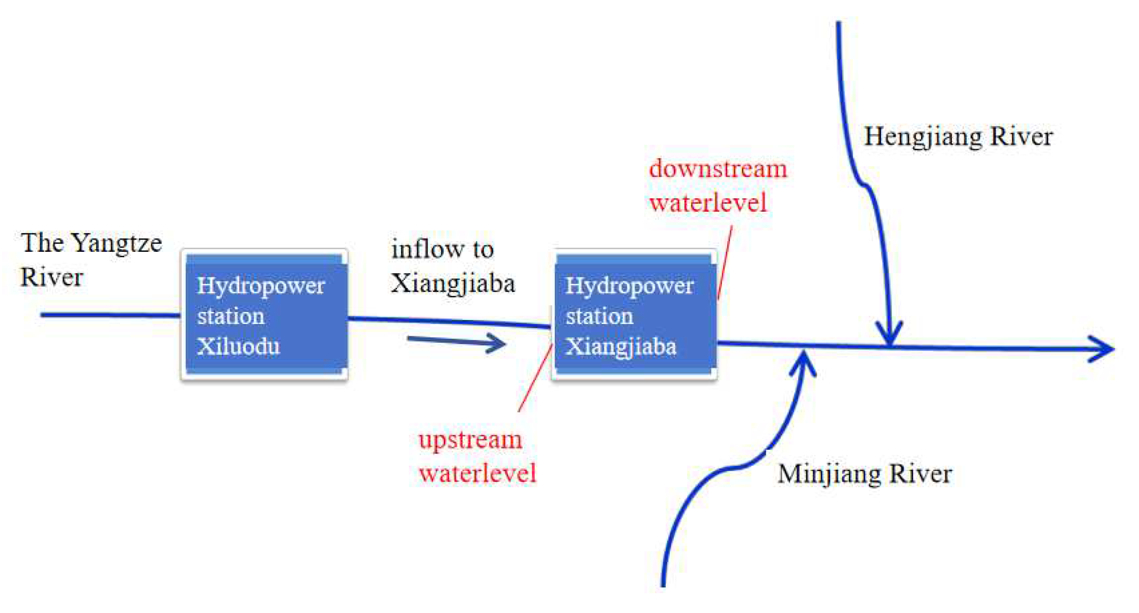
XJB’s geographical location is shown in Figure 1. The dam site of XJB is located at the canyon exit of the lower reaches of Jinsha River[17,18]. The installed capacity of XJB hydropower station is 6million kW, the number of units is 8, the rated output of each unit is 750000 kW, and the maximum capacity of each unit corresponds to the minimum head of 100m. The regulation capacity of the reservoir is 900million m³, the flood control capacity is 903million m³, and the total capacity is 5.163 billion m³. It can be seen from Figure 1 that the upstream water level of XJB hydropower station is vulnerable to the operation of Xiluodu Hydropower Station (XLD), and the downstream is subject to the backwater effect of the confluence of Hengjiang River (HJR) and Minjiang River (MJR). The complex boundary conditions make the prediction of water level by hydrodynamic method or water balance method with large errors[19].

2.2. Data

This study uses the operation data of XJB Hydropower Station from 2015 to 2020 for prediction and analysis. The content and classification of the data are shown in the Table 1.

2.3. Method

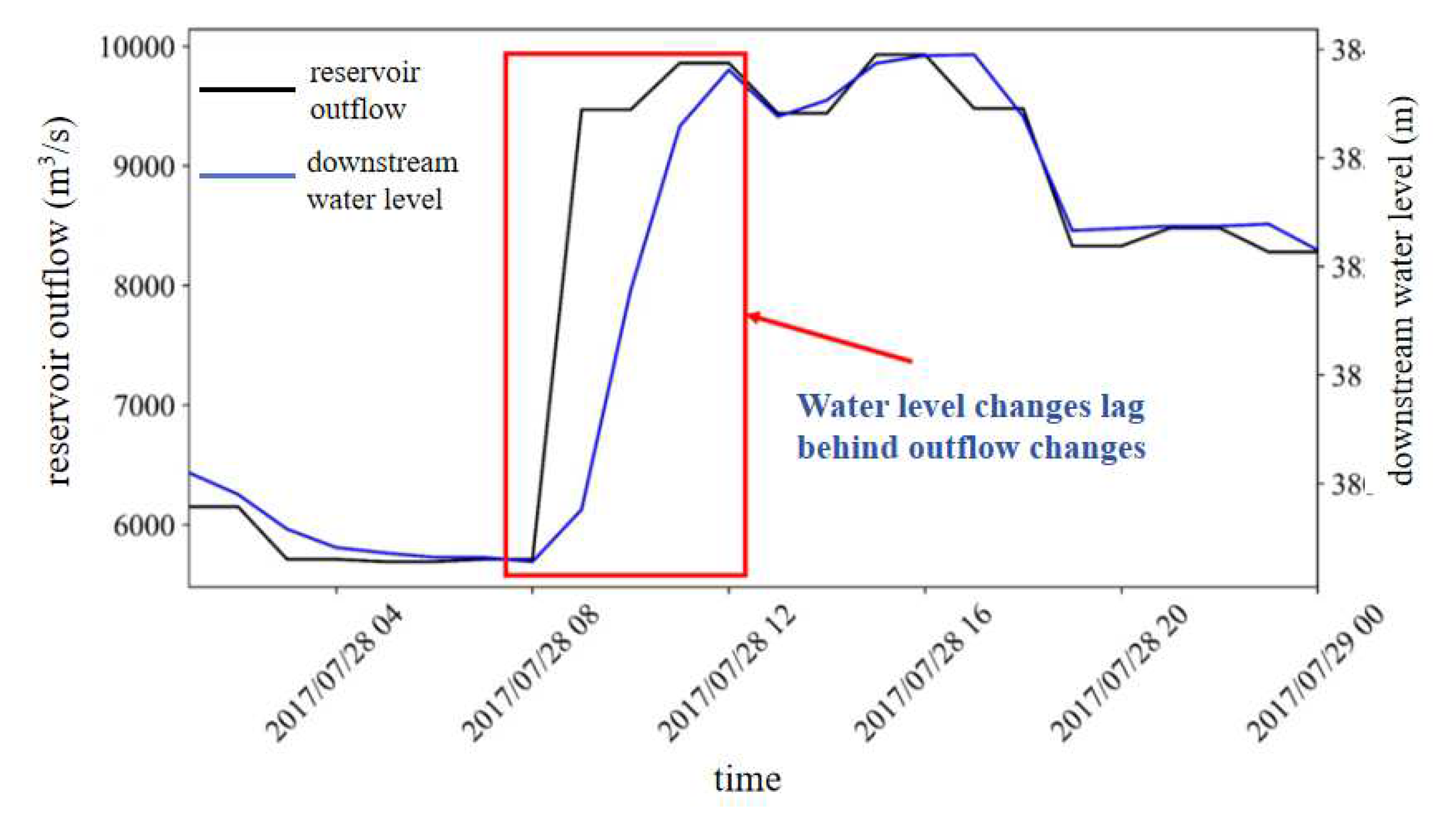
There are many factors affecting the XJB[20]. The most critical factor is the outbound flow of XJB. The change trend of the XJB is consistent with the outbound flow, but there is a lag in time, as shown in Figure 2.

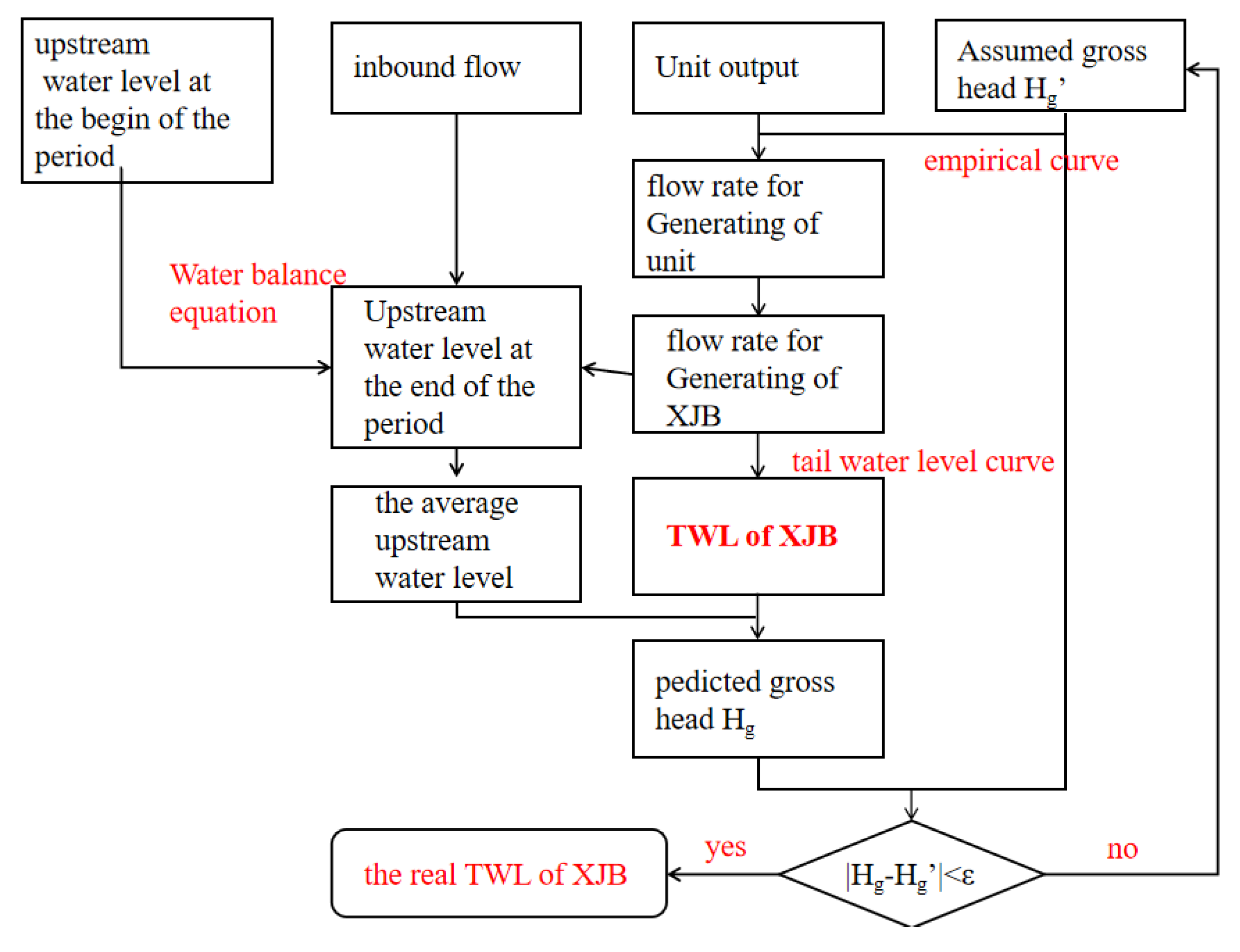
the empirical curve of outbound flow and TWL is usually used to predict the TWL of XJB, which is a characteristic curve based on historical data. The calculation method of outbound flow is to calculate the water balance of XJB reservoir, which delys on the prediction of inbound flow rate and power station output planning in the future. The gross head of the hydropower station is used to query the water consumption rate-gross head empirical curve to obtain the power generation water consumption rate, which is multiplied by the planned output to obtain the power generation flow and outbound flow rate. The calculation process is shown in Figure 3. In this paper, the model constructed by the principle of water balance is called the water balance equation model (WBE model).

However, the factors affecting the water level of XJB Hydropower Station are more complex. The diagram is shown in Figure 3. The water balance method only considers the variables involved in the power station itself, which has two important defects: 1) It fails to consider the operating conditions of the upstream XLD, rainfall between the two hydropower stations, and the impact time lag described above[21]. 2) The Hengjiang river flows in at 1.9km downstream of XJB and the Minjiang River flows in at 28 km downstream of XJB and their backwater effect can not be reflected in the water balance method[22].

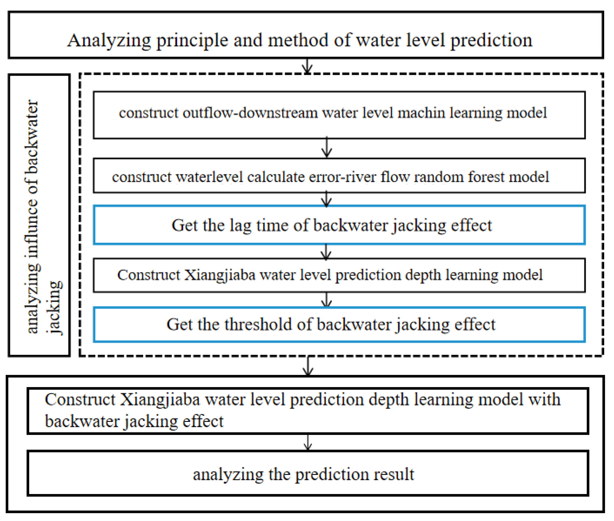
The study will analyze the lag time and threshold of backwater effect using LSTM and machine learning. Based on this, the LSTM prediction model for TWL of XJB considering the impact of backwater effect is constructed.

Firstly, the response relationship between the TWL of XJB and related variables is analyzed and discussed according to the hydrodynamic method and water balance method. Then, the machine learning model for water level prediction in the TWL of XJB is constructed, and the characteristic relationship between the prediction error and the outbound flow of Hengjiang River (HJR) and Minjiang River (MJR) in different periods is analyzed with the help of random forest model, so as to obtain the time lag of backwater effect. Further, a deep learning water level prediction model for the TWL of XJB was established. Different scenarios were divided according to different flow rate of HJR and MJR, and the backwater effect threshold was obtained by observing the prediction results. Finally, a water level prediction model for TWL of XJB considering the impact of backwater effect was constructed. The method roadmap is shown as Figure 4.

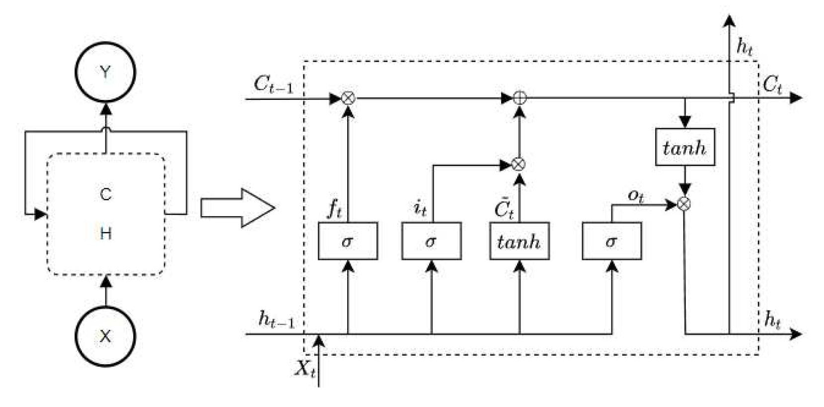
LSTM algorithm is chosen to predict the TWL of XJB due to the response time lag between the multi-variable relations in water level prediction, for it can effectively slow down the gradient disappearance or explosion that may occur in long sequence problems, and perform better than traditional RNNS on longer sequence problems.

LSTM implements the control of information state of memory unit through forget gate and input gate. The forget gate f_t determines which water level influence information of h_t-1 and X_t should be discarded at time t; The input gate it is used to determine how much X_t and h_t-1 water level impact information needs to be passed to C_t at time t in order to update the information stored by C_t-1. LSTM uses the output gate to control the unit state C_t. A_t the current time t, how many water level influence information in h_t-1 and X_t should be output [23,24].

3. Analysis of Backwater Effect

3.1. Analysis Method of Backwater Effect

The lag time analysis is mainly divided into two steps. First, the linear regression model is used to fit the corresponding relationship between the TWL of XJB and the outbound flow, and then the error between the predicted TWL of XJB and the actual TWL is calculated. Further, the corresponding relationship between the TWL prediction error and the flow rate of Hengjiang River (HJR) and Minjiang River (MJR) before different hours is constructed. Taking the flow rate of HJR and MJR in different lag periods as characteristic variables, and the water level prediction error as output variable. The importance of different input factors can be calculated by random forest model, and the flow rate data in which lag period the error mainly comes from can be obtained.

The threshold analysis is based on the results of lag analysis, and establishes a 12 hour prediction model without considering the backwater effect, then we can divide different scenarios according to the different flow rate of HJR and MJR. Calculating the prediction error of water level under different scenarios, and the prediction error of scenarios with flow rate exceeding the backwater effect threshold will be significantly higher than that under the threshold.

3.2. Time Lag Analysis of Backwater Effect

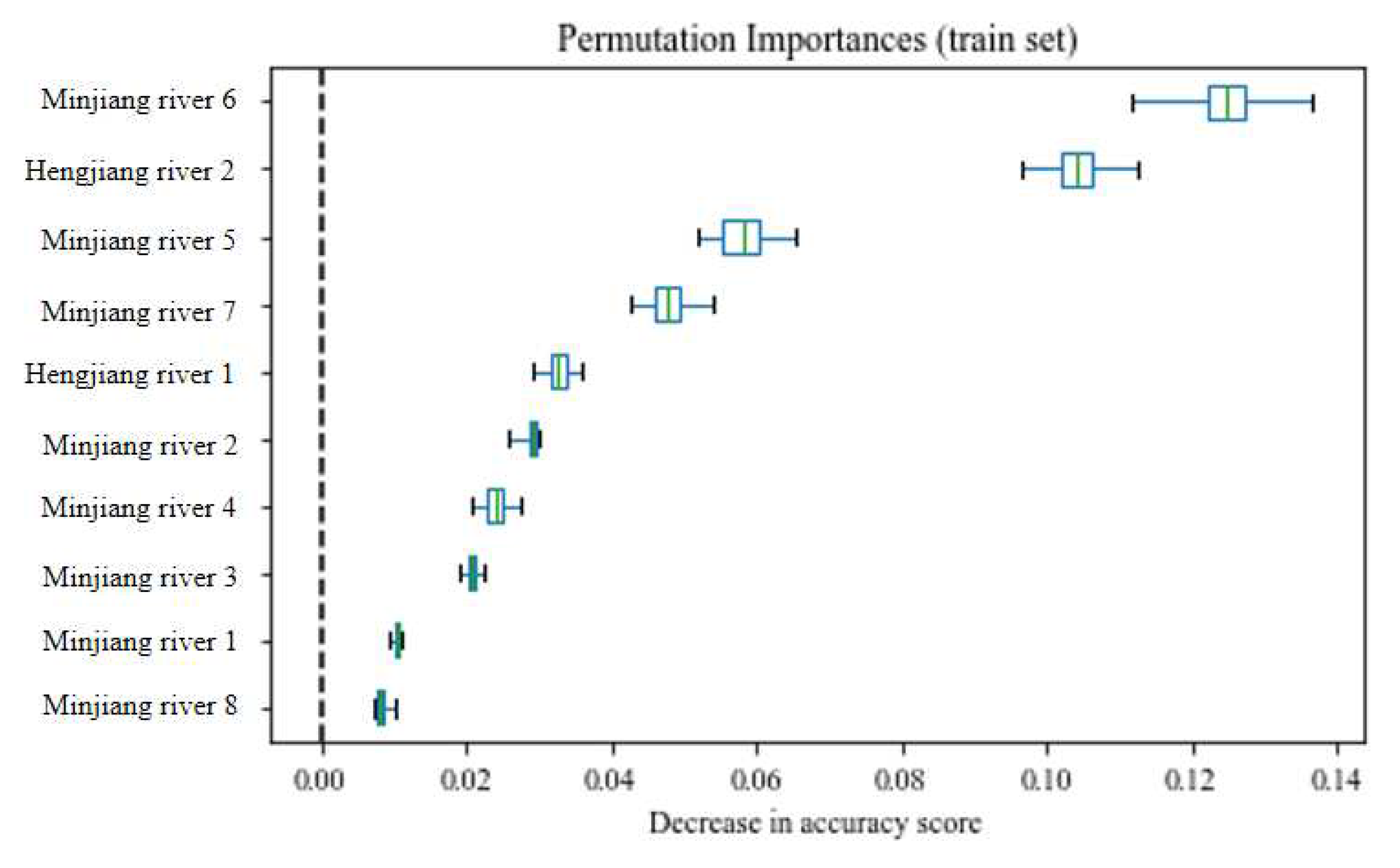
The random forest model analyzes the weight of a feature factor by randomly typing the order of a feature factor in the training set and analyzing its influence on the calculation effect of the output variable. Construct a random forest model with the flow rate of HJR and MJR in different lag periods as the input factor, and the TWL of XJB error calculated by machine learning method as the output. The characteristic weights between the flow rate of HJR and MJR in different lag periods to the water level error can be obtained by the model. The calculation results are shown in Figure 5. The ordinate in the figure shows different input factors. The ‘Minjiang river 6’ represents the flow rate of the HJR six hours ago. Other input factors are similar. The abscissa shows the decline of the model index after randomly disrupting the factor, which can characterize the importance of the disrupted factor to the output variable. In the analysis process, the calculation was repeated for 30 times, and the results were drawn as a box diagram like Figure 6.

It can be seen from the figure that the test set and the training set have the same characteristic importance calculation distribution. The top five factors of the two sets are the same, which are Minjiang river 6, Hengjiang river 2, Minjiang river 5, Minjiang river 7 and Hengjiang river 1. The results show that the lag time of backwater effect of MJR flow rate to TWL of XJB is about 5-7 hours, and that of HJR flow rate to TWL of XJB is about 1-2 hours.

3.3. Threshold Analysis of Backwater Effect

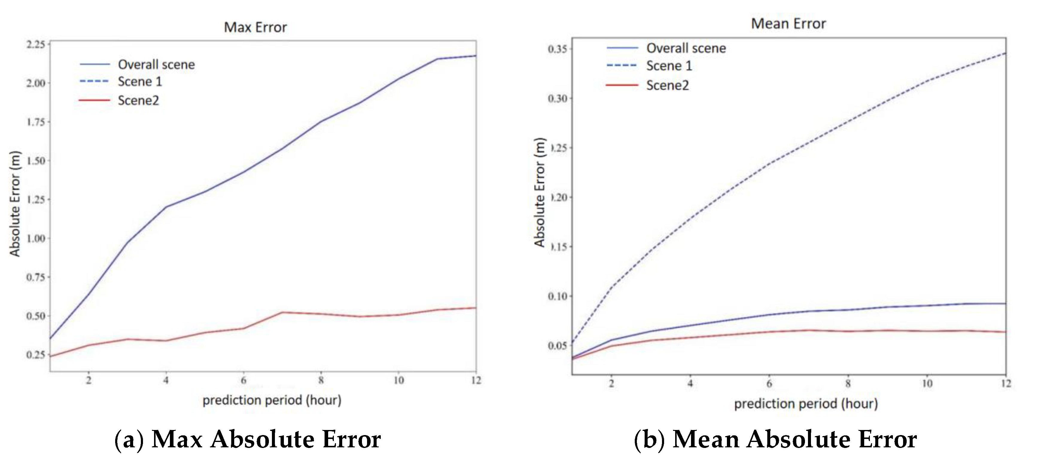
The backwater effect threshold analysis is to predict the TWL of XJB under different scenarios by using a deep learning model without considering backwater effect after dividing the flow scenarios of HJR and MJR. When the flow rate of HJR and MJR in the scenario exceeds the backwater effectt threshold, the prediction error will be much higher than that of the scenario where the flow rate is lower than the backwater effect threshold. Take the data of 2019 for prediction and calculation, and take 700 m³/s as the threshold of the HJR flow rate and 7000 m³/s as the threshold of the MJR flow rate, which are divided into two types of scenarios. Scenario 1: any one of the HJR flow rate and MJR flow rate exceeds the thresholds; Scenario 2: the HJR flow rate and MJR flow rate are both less than the thresholds, and an overall scenario without threshold division. The 12 hour prediction error is shown in the Figure 7:

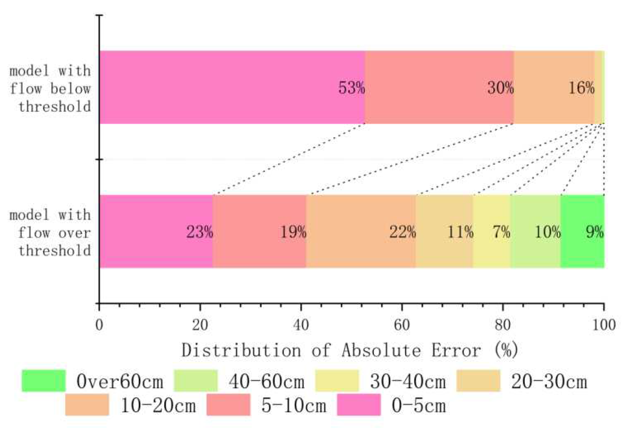
The maximum prediction error of the overall scenario coincides with that of scenario 1, while the average prediction error of scenario 1 is much higher than that of the overall scenario and scenario 2. The error distribution diagram of different scenarios is shown in Figure 8.

From the distribution of errors, in Scenario 1, 18.49% of the errors are above 40 cm, while in Scenario 2, 0.04% of the errors are above 40 cm. Overall, using 700 m³/s as the threshold for HJR flow rate and 7000 m³/s as the threshold for MJR flow rate can significantly distinguish between forecast scenarios. When both flow rate are less than the threshold, the maximum prediction error is 55.02 cm, and the average prediction error is 5.93 cm. In comparison, it can be approximately assumed that this scenario is not affected by the backwater effect.

4. Analysis of Predictive Performance

4.1. Prediction Result of WBE Model

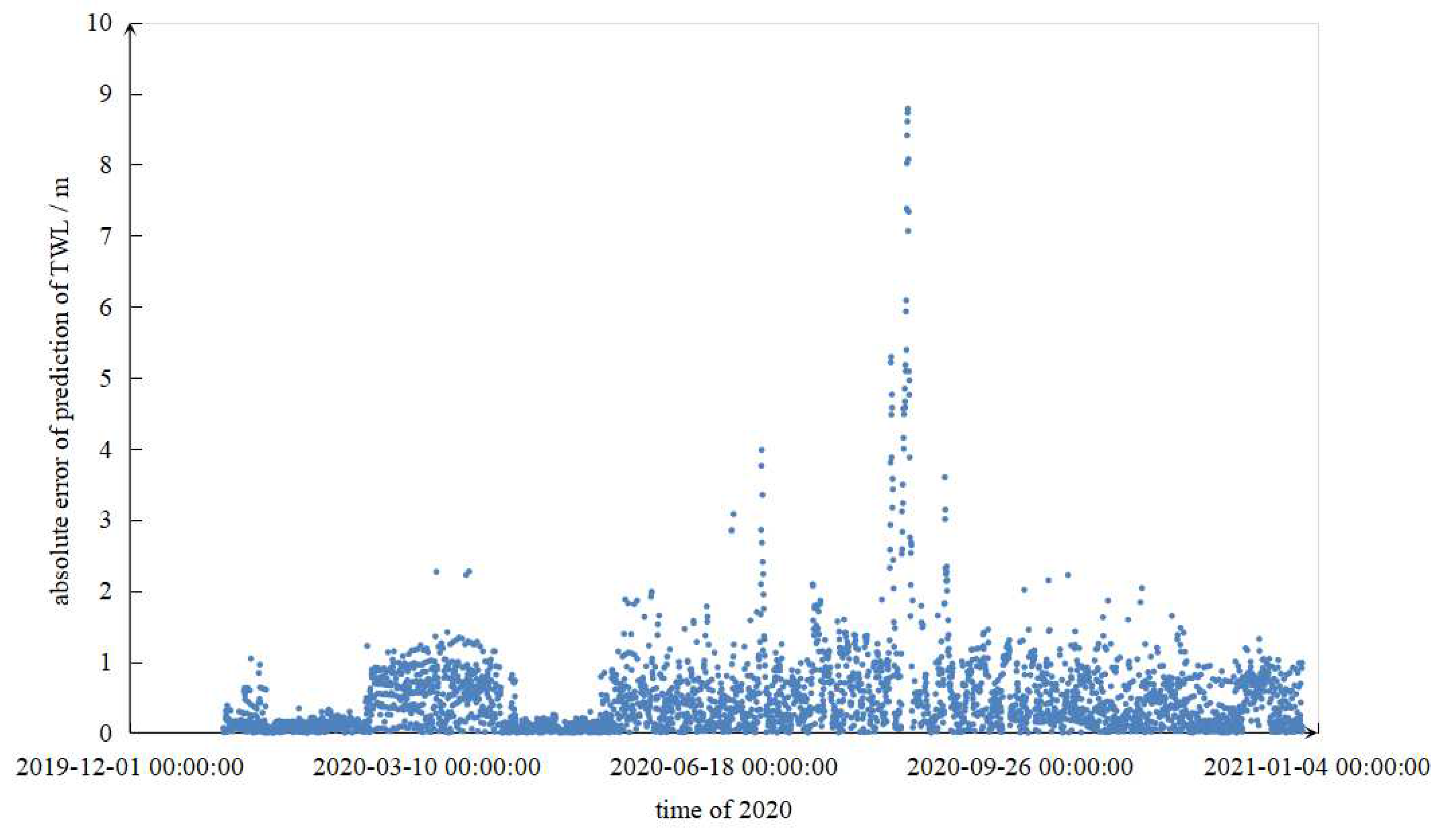
By using the water balance model idea mentioned above, the WBE model is constructed to calculate the water level at the tail of Jiaba in 2020 with a two-hour step length. The absolute error is shown in Figure 9:

The average absolute error of the result is 47.3 cm, the maximum absolute error is 878.3 cm, and the absolute error above 100 cm accounts for about 10%. In the calculation process, it is found that the error of the discharge flow out of XJB is less than 3%, which is highly accurate. Therefore, most of the calculation error of the TWL of XJB comes from the inaccuracy of the TWL empirical curve and the backwater effect of HJR and MJR under XJB dam.

4.2. Prediction Result of LSTM Model

The model in the backwater effect threshold analysis does not consider the impact of rainfall in the stream direction interval, and directly takes the inflow of XJB as the input, which is difficult to be applied in the actual prediction. Therefore, the inflow of XJB is replaced by XLD output, XLD abandoned water and rainfall in the stream direction interval to construct a prediction model that can be applied in practice. The characteristic variables considered in the model include:

Table 2. The content of characteristic variables considered in deep learning models.

period	characteristic variable
History datas	XJB upstream and downstream water levels, Rainfall among XLD and XJB, Pengshan and MJR rainfall, HJR rainfall, HJR flow rate, MJR flow rate, XJB inflow, XJB output, XJB abandon flow
Future datas	Rainfall among XLD and XJB, XLD and XJB output, XLD and Xiangjiaba abandon flow, HJR flow rate, MJR flow rate

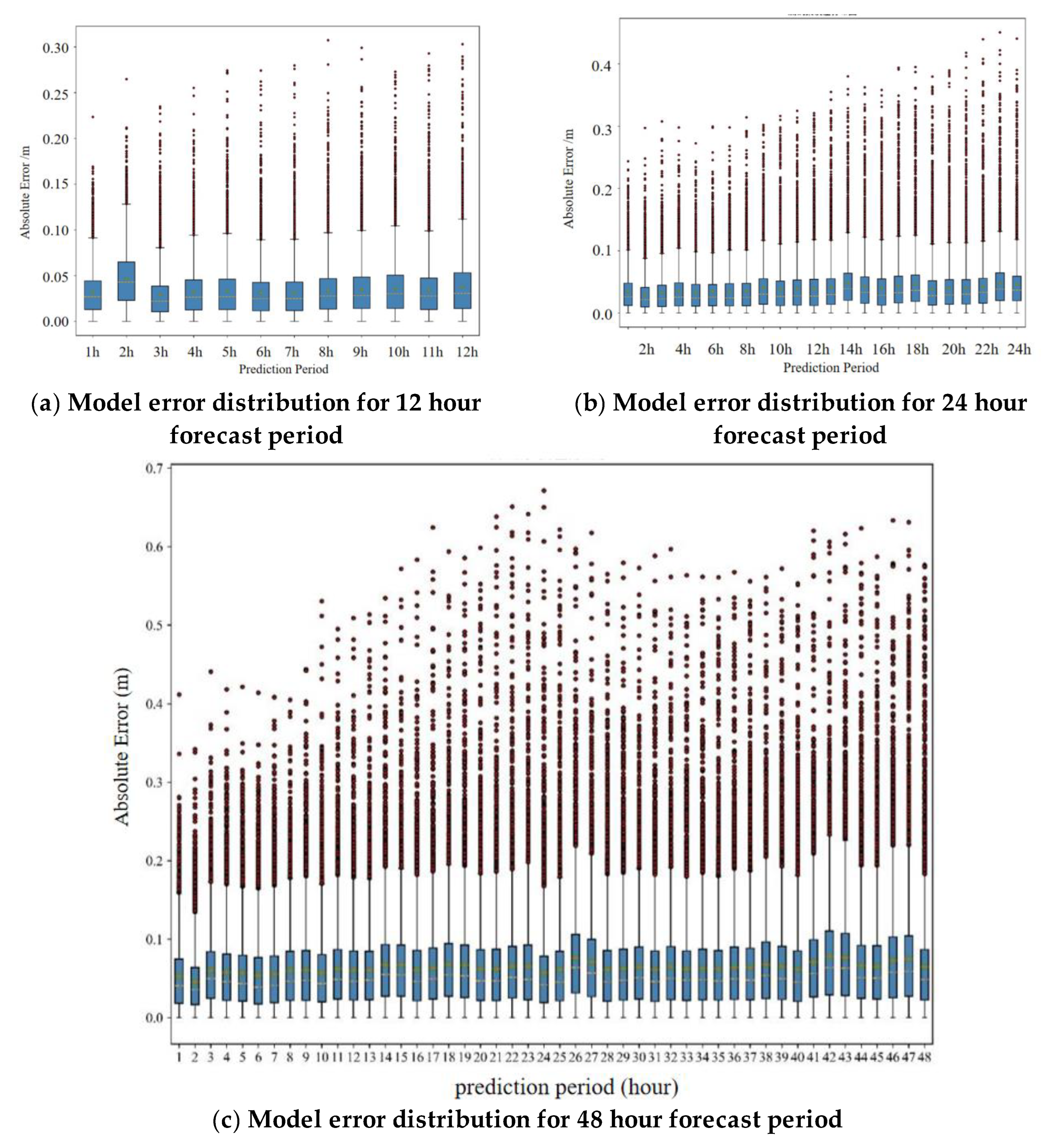
The model used forecast data, but the forecast data itself contains errors, and the impact of the errors on the water level prediction is unknown. The backwater effect of HJR and MJR, and the transformation of rainfall into runoff and inflow have time lag. Therefore, when the forecast period of the model is short, the measured historical flow rate and rainfall data of HJR, MJR and XJB can provide prediction support for the model and make the model more practical. In order to compare the prediction effects of the models with different forecast periods, this paper constructs three prediction models of XJB’s TWL with different forecast periods of 12 hours, 24 hours and 48 hours with step of 1 hour. The error statistics of different forecast periods are shown in the Figure 10.

The error distribution of each model in different forecast periods is basically similar, and get no significant exception. From the comparison between the models, the prediction effect of the 12-hour forecast model is the best on the whole, with an average absolute error of 3.43 cm and a maximum absolute error of 30.74 cm, which are lower than the error of the previous 12 hours forecast of the 24-hour forecast model. The average absolute error is 3.56 cm and the maximum absolute error is 32.47 cm. The average absolute error of the 24-hour forecast model is 3.93 cm and the maximum absolute error is 45.07 cm, which is lower than the average absolute error of 6.03 cm and the maximum absolute error of 67.14 cm in the previous 24 hours of the 48-hour forecast model. Therefore, in the final prediction, a comprehensive forecast from three different models is adopted. These models are the first 12-hour forecast from the 12-hour prediction model, the 13 to 24-hour forecast from the 24-hour prediction model, and the 25 to 48-hour forecast from the 48-hour prediction model.

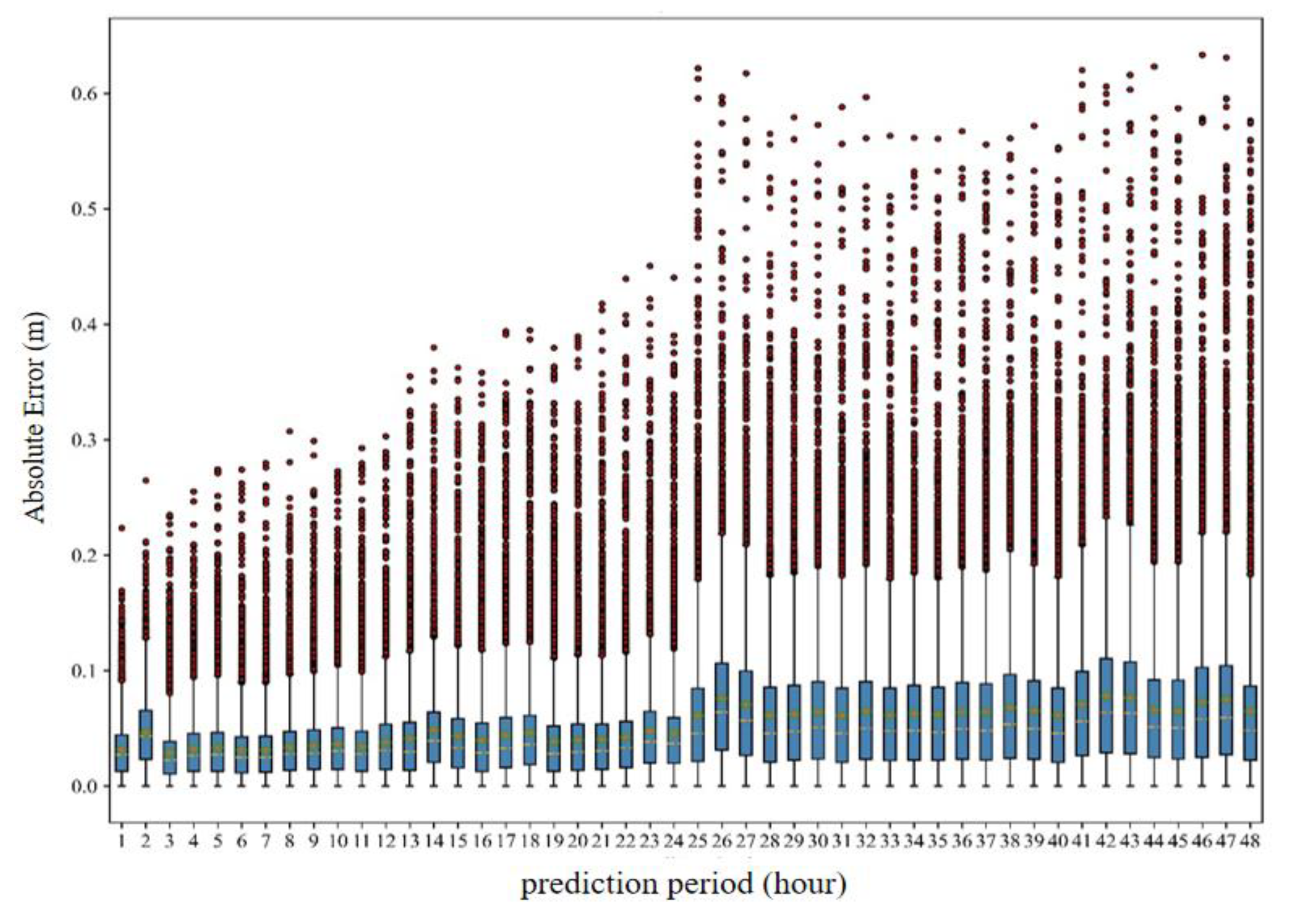
Based on the prediction models of different forecast periods, the overall error distribution within the 48 hour forecast period is shown in the Figure 11.

From the graph, it can be seen that the prediction error in the last 24 hours is significantly higher than that in the first 24 hours, with the average absolute error increasing from 3.87 cm in the first 24 hours to 6.67 cm in the latter 24 hours, and the maximum absolute error increasing from 45.07 cm in the first 24 hours to 63.35 cm. The mean absolute error of the overrall result is 5.27 cm.

4.3. Result Analysis

Compare with the WBE model’s prediction result, the mean absolute error of LSTM model considering the backwater effect is about 11%. The prediction accuracy of LSTM model is much higher than that of WBE model.

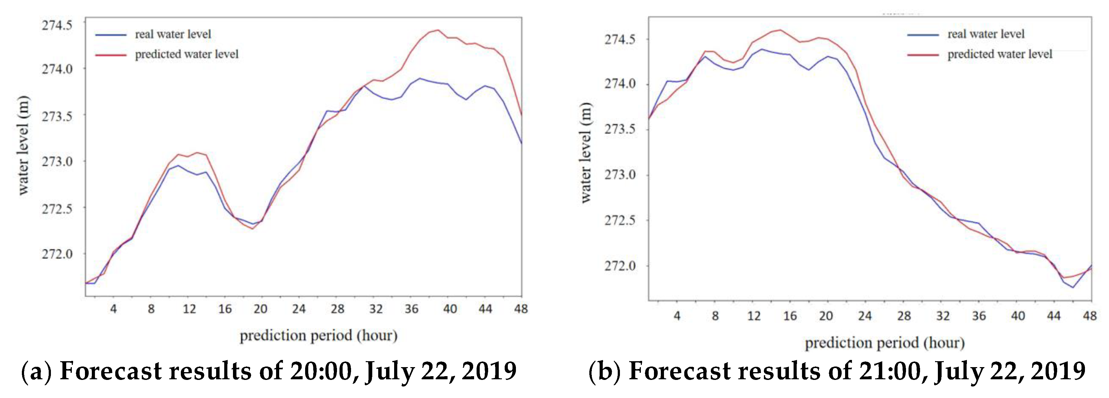
Take the case with error more than 60 cm for analysis, and the comparison between the predicted water level process and the measured water level process is shown in Figure 12 (a). When the prediction start time is delayed by one day, that is, the prediction starts at 21:00 on July 22nd, 2019, the comparison between the predicted water level process and the measured process is shown in Figure 12 (b). It can be seen that the overall error decreases and the maximum water level prediction error decreases. Therefore, in the process of practical application, rolling prediction can be used to reduce the impact of prediction error.

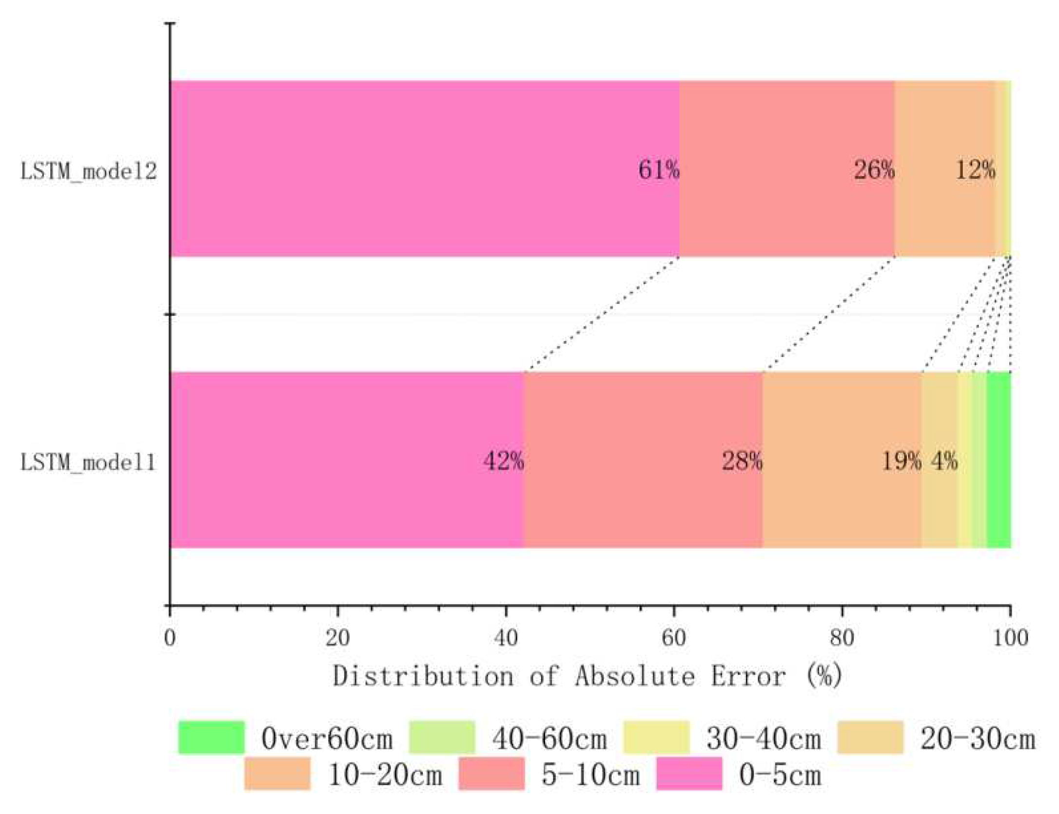
Compare the prediction results of the LSTM prediction model without considering backwater effect constructed in Chapter 3 with the prediction model considering backwater effect constructed in this chapter, and label the model without considering the backwater effect as LSTM_ Model1, another one labeled as LSTM_ Model2. The error distribution of the predicted results between the two is shown in the Figure 13：

The prediction error of the two models is shown in the following table, and the maximum absolute error and mean absolute error have significantly decreased after considering the backwater effect. The mean absolute error was reduced from 7.66 cm to 5.272 cm, and the maximum absolute error was reduced from 217.52 cm to 63.35 cm.

Table 3. Error comparison of whether the model considers the backwater effect.

	mean absolute error	maximum absolute error
LSTM_model1	7.66	217.52
LSTM_model2	5.27	63.35

5. Conclusions

The application of deep learning method is flexible. Thanks to its powerful computing power, we can not only input characteristic variables for direct calculation of water level prediction, but also use it to make many characteristic analysis. This paper analyzed the threshold and lag time of the HJR and MJR’s backwater effect to TWL of XJB with the using of deep learning, and constructed the LSTM prediction model considering the backwater effect. The accuracy of the prediction result is improved by about 90% compared with the water balance algorithm model, and by about 30% compared with the deep learning model without considering the backwater effect. The prediction error is controlled within 63 cm. It is proved that the deep learning method and neural network model have a good application prospect in the field of water resources, and are a reliable alternative to the traditional calculation ideas.

Acknowledgement

This research was funded by the National Key Research and Development Program of China（No.2022YFC3202300）, the National Natural Science Foundation of China (No.42271044，51979114, 42207526), the Fundamental Research Funds for Central Public Welfare Research Institutes (CKSF2021486), the Scientific Research Project of China Three Gorges Corporation (0704106), and the Major science and technology project of the Ministry of Water Resources (SKS-2022128), the Natural Science Foundation of Hubei Province (No.2022CFD164).

References

Ahn J, Na Y, Park W S. Development of Two-Dimensional Inundation Modelling Process using MIKE21 Model[J]. KSCE Journal of Civil Engineering 2019, 23.
Zhu S, Hrnjica B, Ptak M, et al. Forecasting of water level in multiple temperate lakes using machine learning models[J]. Journal of Hydrology 2020, 585, 124819.
Zhongyao L.Simulate the forecast capacity of a complicated water quality model using the long short-term memory approach[J].Journal of Hydrology 2020, 581. [CrossRef]
Choi C, Kim J, Han H, et al. Development of water level prediction models using machine learning in wetlands: A case study of Upo wetland in South Korea[J]. Water 2019, 12, 93. [CrossRef]
Wang D , Qi X , Wen S ,et al. Robust nonlinear control and svm classifier based fault diagnosis for a water level process. ICIC Express Letters 2015, 9, 767–774.
Haijiao D, Wengang C. Prediction Model of River Water Level Based on LS-SVM[C]//International Conference on Intelligent Computation Technology & Automation. IEEE Computer Society 2015. [CrossRef]
Wang H, Song L.Water Level Prediction of Rainwater Pipe Network Using an SVM-Based Machine Learning Method[J]. International Journal of Pattern Recognition and Artificial Intelligence 2019, 34. [CrossRef]
B J Z A , C X W , D C Z A ,et al. Application of cost-sensitive LSTM in water level prediction for nuclear reactor pressurizer - ScienceDirect. Nuclear Engineering and Technology 2020, 52, 1429–1435. [CrossRef]
Wunsch A, Liesch T, Broda S.Groundwater level forecasting with artificial neural networks: a comparison of long short-term memory (LSTM), convolutional neural networks (CNNs), and non-linear autoregressive networks with exogenous input (NARX)[J]. Hydrology and Earth System Sciences 2021, 25. [CrossRef]
Li X, Liu B, Wang Y,et al. The hydrodynamic and environmental characteristics of tributary bay influenced by backwater jacking and intrusion of main reservoir[J]. 2020. [CrossRef]
Shuofeng L , Puwen L , Koyamada K .LSTM Based Hybrid Method for Basin Water Level Prediction by Using Precipitation Data. Journal of Advanced Simulation in Science and Engineering 2021, 8, 40–52. [CrossRef]
Zhang Z, Qin H, Yao L,et al. Downstream Water Level Prediction of Reservoir based on Convolutional Neural Network and Long Short-Term Memory Network[J].Journal of Water Resources Planning and Management, 2021, 147.
Nourani V .Reply to comment on 'Nourani V, Mogaddam AA, Nadiri AO. 2008. An ANN-based model for spatiotemporal groundwater level forecasting. Hydrological Processes 22: 5054–5066'. Hydrological Processes 2010, 24, 370–371. [CrossRef]
Kochhar A, Singh H, Sahoo S,et al.Prediction and forecast of pre-monsoon and post-monsoon groundwater level: using deep learning and statistical modelling[J]. Modeling Earth Systems and Environment, 2022, 8.
Litrico X, Belaud G, Baume J P, et al. Hydraulic modeling of an automatic upstream water-level control gate. 2005, 131, 176–189.
Bazartseren B, Hildebrandt G, Holz K P. Short-term water level prediction using neural networks and neuro-fuzzy approach. Neurocomputing 2003, 55, 439–450. [CrossRef]
Yan H U.Reservoir sediment computation of Xiangjiaba hydropower plant[J]. Yangtze River, 2003.
Wei-Min M A, Ding-Zhen N, Yan-Ming C.Key Technical Schemes for ±800kV UHVDC Project from Xiangjiaba to Shanghai[J].Power System Technology, 2007. [CrossRef]
Qiao, Qi, Wang, et al.Short-term hydro generation scheduling of Xiluodu and Xiangjiaba cascade hydropower stations using improved binary-real coded bee colony optimization algorithm[J].Energy conversion & management, 2015.
Choi C, Kim J, Han H, et al. Development of water level prediction models using machine learning in wetlands: A case study of Upo wetland in South Korea. Water 2019, 12, 93. [CrossRef]
Yunping Y , Mingjin Z , Zhaohua S ,et al. The relationship between water level change and river channel geometry adjustment in the downstream of the Three Gorges Dam. Journal of Geographicl Science 2018, 28, 19. [CrossRef]
Guangjing C, Zhiguo C.Research and Application of Optimized Model for Long-term Daily-operation of the Three Gorges & Gezhouba Cascade Power Stations[C]//International symposium on Three Gorges Project and water resources development and protection of Yangtze River.Vice President, CTGPC;Head of Science & Environmental Department, CTGPC;, 2010.
Wang B, Liu S, Wang B,et al. Multi-step ahead short-term predictions of storm surge level using CNN and LSTM network[J].Acta Oceanologica Sinica, 2021. [CrossRef]
Jung S, Cho H, Kim J, et al. Prediction of water level in a tidal river using a deep-learning based LSTM model. Journal of Korea Water Resources Association 2018, 51, 1207–1216.

Figure 1. Schematic diagram of upstream and downstream of XJB.

Figure 2. XJB outbound flow and tail water level change process chart.

Figure 3. Calculating process of XJB by water balance method.

Figure 4. Flow chart of research ideas.

Figure 5. Schematic diagram of LSTM calculation steps.

Figure 6. Characteristic importance of different input factors.

Figure 7. Max error and mean error of different scenarios.

Figure 8. Destribution of absolute error of models with different flow rate.

Figure 9. Annual distribution of absolute error of XJB’s TWL predicted by WBEmodel.

Figure 10. Model error distribution for different hour forecast period.

Figure 11. Overall predict error.

Figure 12. Case analysis of XJB’s TWL predicion.

Figure 13. Comparison of prediction error whether the model considers the backwater effect.

Table 1. Data type and their time.

Data type	station	Time series	Time step
water level	upstream water level and tail water level of XJB	2015-2020	2 hours, 1 hour,
flow rate	XLD and XJB’s outbound flow rate, inbound flow rate and abandon flow rate, HJR and MJR flow rate	2015-2020	1 hours
output	XLD, XJB plant, branch plant, and each unit output	2015-2020	2 hours, 1 hour,
empirical curve	XLD and XJB’s water level-storage curve, head loss curve, unit flow rate curve, tail water level curve, etc	/	/

Disclaimer/Publisher’s Note: The statements, opinions and data contained in all publications are solely those of the individual author(s) and contributor(s) and not of MDPI and/or the editor(s). MDPI and/or the editor(s) disclaim responsibility for any injury to people or property resulting from any ideas, methods, instructions or products referred to in the content.

© 2023 by the authors. Licensee MDPI, Basel, Switzerland. This article is an open access article distributed under the terms and conditions of the Creative Commons Attribution (CC BY) license (http://creativecommons.org/licenses/by/4.0/).

Copyright: This open access article is published under a Creative Commons CC BY 4.0 license, which permit the free download, distribution, and reuse, provided that the author and preprint are cited in any reuse.

MDPI Initiatives

Important Links

Choose an area of interest and we will send you notifications of new preprints at your preferred frequency.

Disclaimer