Preprint
Article

Morlet Wavelet Neural Network Investigations to Present the Numerical Investigations of the Prediction Differential Model

Altmetrics

Downloads

88

Views

38

Comments

0

A peer-reviewed article of this preprint also exists.

Submitted:

04 October 2023

Posted:

05 October 2023

You are already at the latest version

Alerts
Abstract
In this study, a design of Morlet wavelet neural networks (MWNNs) is presented to solve the prediction differential model (PDM) using the global approximation capability of genetic algorithm (GA) and local quick interior-point algorithm scheme (IPAS), i.e., MWNN-GAIPAS. The famous PDM is known as a variant of functional differential system that works as an opposite of the historical delay differential models. A fitness function is optimized using the mean square error by applying the GA-IPAS for solving the PDM. Three PDM examples have been presented numerically to check the authenticity of the MWNN-GAIPAS. For the perfection of the designed MWNN-GAIPAS, the comparability of the obtained results and exact results is performed. Moreover, the neuron analysis is performed by taking the 3, 10 and 20 number of neurons. The statistical observations have been performed to authenticate the reliability of the MWNN-GAIPAS for solving the PDM.
Keywords: 
Subject: Computer Science and Mathematics  -   Applied Mathematics

1. Introduction

The study of the prediction differential model (PDM) is considered very significant for the researchers due to various applications in climate forecasting, biological systems, stock markets, transport, astrophysics, and engineering, etc. The sense of delay differential model (DDM) that presents a historical system has been applied to design the form of PDM. The idea of DDM introduced by Newton and Leibnitz that has been presented few centuries ago and has widely been applied in many applications of engineering, economical systems, population dynamics, communication and transport networks [1,2,3,4,5]. Many researchers applied different techniques to solve the DDM, e.g., Bildik et al [6] implemented to solve DDM using the optimal perturbation iterative scheme. Rahimkhani et al [7] presented an approach in order to solve the fractional form of DDM. Sabir et al [8] presented a new multi-singular nonlinear system with the delayed factors. Aziz et al [9] used Haar wavelet approach for solving the partial form of DDM. Frazier [10] implemented the wavelet Galerkin method to solve the DDM of the second kind. Tomasiello [11] solved a famous class of the historical DDM by applying the fuzzy transform method. Vaid [12] implemented the trigonometric B-spline approach to solve the second kind of singularly perturbed based DDM. Hashemi et al [13] solved the fractional pantograph delay system by an efficient computational approach. Adel et al [14] discussed the solutions of pantograph singular DDM using the Bernoulli collocation scheme. Erdogan et al [15] worked to solve perturbed singularly DDM using a well-known finite difference approach. The DDM is a second order differential model, which is given as [16]:
{ y ( t ) = f ( t , y ( t ) , y ( t γ 1 ) ) , γ 1 > 0 , c t b , y ( t ) = θ ( t ) , σ t c , 0 γ 1 | c σ | , y ( c ) = w ,
where γ 1 , θ ( t ) indicate the delayed factor and initial conditions. The delayed form y ( t γ 1 ) shows in the above model, which is to subtract in time t, i.e., c t b . σ is a small constant and w is value derivative of y . The prediction form of the DDM is achieved by adding some terms in t, i.e., y ( t + γ ) , with prediction term γ . The literature form of the mathematical PDM is given as [17,18]:
{ y ( t ) = f ( t , y ( t ) , y ( t + γ ) ) , γ 1 > 0 , c t b , y ( t ) = θ ( t ) , σ t c , 0 γ 1 | σ c | , y ( c ) = w ,
The above mathematical PDM shown in equation (2) has been designed recently and never been solved by functioning the universal approximation ability of Morlet wavelet neural network (MWNN) together with the global and local search optimizations of genetic algorithm (GA) and interior-point algorithm scheme (IPAS), i.e., MWNN-GAIPAS. The numerical investigations have been performed by using the MWNN-GAIPAS by taking 3, 10 and 20 numbers of neurons. Recently, the stochastic computing solvers have been used to exploit the corneal shape nonlinear system [19], nonlinear doubly singular model [20], system of Emden–Fowler model [21], nonlinear model SIR based dengue fever [22], functional differential singular systems [23,24], HIV infection based CD4+ T cells [25], Thomas-Fermi system [26], prey-predator models [27], stiff nonlinear models [28], fractional multi-singular differential models [29,30], heat conduction based human head system [31] and singular nonlinear system of third kind [32]. These above performances of the stochastic solvers authenticate the worth in terms of robustness, convergence and precision. Based on the above applications, the authors are inspired to present the solutions of the PDM by using the universal approximation ability of MWNN together with the optimization procedures of GAIPAS. Few noticeable, prominent and salient measures of the current study are summarized as:
  • A layer structure of MWNNs is designed and optimization is performed through integrated neuro-evolution based heuristic with IPAS to solve the PDM numerically.
  • The analysis with 3, 10 and 20 numbers of neurons is presented to interpret the stability and accuracy of the designed approach for solving the PDM.
  • The proposed MWNN-GAIPAS is executed for three different examples based on PDMand comparison is performed with the exact solutions to validate the accurateness of proposed MWNN-GAIPAS.
  • Statistics investigations through different performances of fitness, “root mean square error (R.MSE)”, “variance account for (VAF)”, “Theil’s inequality coefficients (TIC)” and semi inter quartile range (S.I.R) further authenticate the MWNN-GAIPAS for solving all examples of the PDM.
  • The complexity performance of the MWNN-GAIPAS based on 3, 10 and 20 numbers of neurons using different statistical operators is examined for all the examples of the PDM.
  • The proposed MWNN-GAIPAS provides reasonable and accurate results in training span. Furthermore, smooth processes of implementation, constancy, and expendability are other obvious applauses.
The organization of the paper is as follows: Section 2 provides the detail of the design MWNN-GAIPAS. Performance procedures are given in Section 3. Results are provided in Section 4. Conclusions along with upcoming reports of the research are provided in final Section.

2. Methodology: MWNN-GAIPAS

The proposed methodology based on the MWNN-GAIPAS to solve each example of the PDM is separated into two phases.
  • An error-based merit function is presented to construct the MWNNs.
  • For the optimization of the merit function, the hybrid form of GAIPAS is described for the decision variables of MWNNs.

2.1. MWNN Modeling

The ability of the NNs using the MW function is used to present the stable, steady and reliable outcomes in many areas. The PDM mathematical form given in equation (2) is stated with feed forward NNs including the derivatives in input, hidden and output layers as:
y ^ ( t ) = k = 1 s q k v ( w k t + m k ) , y ^ ( n ) = k = 1 s q k v ( n ) ( w k t + m k ) .
In the above network, s represents the neurons, W = [ q , w , m ] is the unknown weight vector, i.e., q = [ q 1 , q 2 , , q s ] , w = [ w 1 , w 2 , , w s ] a n d m = [ m 1 , m 2 , , m s ] . The MWNN is not implemented before to present the numerical solutions of PDM, mathematically given as [33]:
v ( t ) = cos ( 4 3 t ) e ( 1 2 t 2 )
Eq. (3) takes the form as:
y ^ ( t ) = k = 1 s q k cos ( 4 3 ( w k t + m k ) ) e 1 2 ( w k t + m k ) 2 , y ^ ( t ) = k = 1 s q k w k e 1 2 ( w k τ + m k ) 2 ( sin { 4 3 ( w k τ + m k ) } + 4 3 ( w k τ + m k ) cos { 4 3 ( w k τ + m k ) } ) , y ^ ( t ) = i = 1 s q k w k 2 e 1 2 ( w k t + m k ) 2 ( 3.0625 cos { 4 3 ( w k t + m k ) } + 7 2 ( w k t + m k ) sin { 4 3 ( w k t + m k ) } + { 1 + ( w k t + m k ) 2 } cos { 4 3 ( w k t + m k ) } ) ,
A merit function E is defined as:
E = E 1 + E 2 ,
where E 1 and E 2 are the unsupervised error based on differential model and boundary conditions, shown as:
E 1 = 1 N m = 1 N ( y m f ( t m , y m , y ( t m + γ ) ) , 0 t m 1 ,
where N h = 1 , v ^ k = v ( τ k ) , y ^ k = y ( t k ) and t m = m h .
E 2 = 1 2 ( y ^ 0 a 1 ) 2 + 1 2 ( y ^ N w ) 2 .

2.2. Optimization process: GAIPAS

The optimization through MWNN is accomplished to solve all the examples of the PDM using the computing hybrid construction of GA and IPAS, i.e., GAIPAS.
Genetic Algorithm is a reliable global search method, which is applied to unconstrained, nonlinear systems using its important operators called selection, elitism, crossover, and mutation. Recently, GA is used in extensive applications in heart disease diagnosis model [34], economic and environmental multi-objective based optimization of a household level of renewable energy [35], power and heat economic dispatch models [36], nonlinear singular system arising in astrophysics [37], prediction of air blast [38], SITR system based COVID-19 [39], three-point boundary value systems of second kind [40] and monorail vehicle based dynamical system [41]. These recent, potential citations inspired the authors to use the global search GA process to achieve the decision variables of MWNNs for solving the PDM.
Interior-point algorithm scheme is a well-known local search mechanism implemented for the convex optimization systems. IPAS does work to solve the optimization problems of both type constrained and unconstrained. Recently, IPAS is used in image restoration [42], nested-constraint resource allocation problems [43], power system state estimation [44], risk-averse PDE-constrained optimization problems [45] and monotone weighted linear complementarity problems [46].
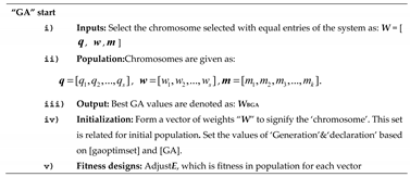
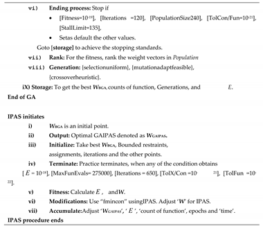
The hybridization is performed to regulate the sluggishness of GA with the IPAS through the optimization procedure. The detail of the hybridization of GAIPAS is provided in the Table 1.
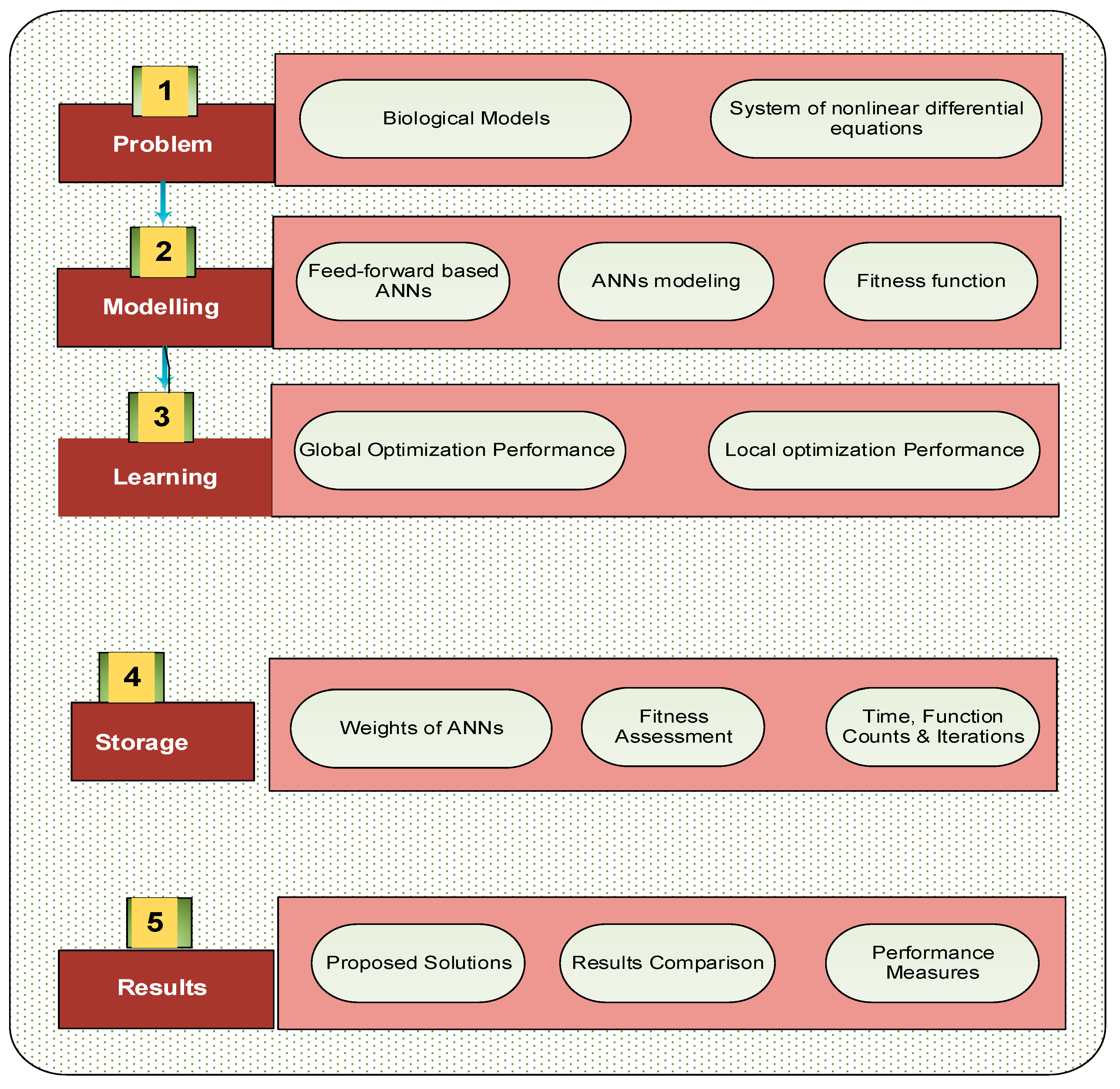
Figure 1. Structure of MWNN-GAIPASfor solving the PDM.
Preprints 86981 g001

3. Statistical performances

The statistical measures are presented based on root mean square error (R.MSE)”, “variance account for (VAF)” and “Theil’s inequality coefficients (TIC)” and S.I.Rtogether with global arrangements of Global R.MSE, VAF and TIC as:
R M S E = 1 s i = 1 s ( y i y ^ i ) 2 ,
{ V A F = ( 1 var ( y i y ^ i ) var ( y i ) ) × 100 , E - VAF = [ | 100 VAF | ] ,
T I C = 1 s i = 1 s ( y i y ^ i ) 2 ( 1 s i = 1 s y i 2 + 1 n i = 1 s y ^ i 2 ) ,
{ S . I   R = 1 2 × ( q 1 q 3 ) , q 1 & q 3 = 1 s t & 3 r d   quartiles .

4. Simulations of the results

The comprehensive form of the solutions based three examples of the PDM are presented in this section.
Example I: Consider
{ 2 y ( t ) y ( t + π ) + y ( t ) = 0 , y ( 0 ) = 1 , y ( 0 ) = 1.
The exact form Eq. (13) is sin t + 1 , while the fitness function is shown as:
E = 1 N i = 1 N ( 2 y ^ i + y ^ i y ^ ( t i + π ) ) 2 + 1 2 ( ( y ^ 0 1 ) 2 + ( y ^ 0 1 ) 2 ) .
ExampleII: Consider the trigonometric PDM based problem is given as:
{ y ( t ) y ( t + 1 ) + y ( t + 1 ) + y ( t ) + cos ( 1 + t ) sin ( 1 + t ) = 0 , y ( 0 ) = 0 , y ( 0 ) = 1.
The exact form of the above model (15) is S i n ( t ) and the merit function is given as:
E = 1 N i = 1 N ( y ^ i y ^ ( t i + 1 ) + y ^ ( t i + 1 ) + y ^ ( t i ) + cos ( 1 + t i ) sin ( 1 + t i ) ) 2 + 1 2 ( ( y ^ 0 ) 2 + ( y ^ i 1 ) 2 ) .
Example III:Consider the PDM based equationis given as:
{ y ^ ( t ) + y ( t + 1 ) y ( t ) 2 t = 0 , y ( 1 ) = 0 , y ( 0 ) = 2.
The exact form of the above model (17) is t 2 3 t + 2 and the merit function is given as:
E = 1 N i = 1 N ( y ^ i y ^ ( t i ) + y ^ ( 1 + t i ) 2 t i ) ) 2 + 1 2 ( ( y ^ 0 2 ) 2 + ( y ^ N ) 2 ) .
The prediction terms are y ( t + 1 ) , y ( t + π ) and y ( t + 1 ) in the above examples. The optimization of each example using the MWNN-GAIPAS for forty independent executions to assess the parameters of the system. The best weight set is accessible to authenticate the proposed outcomes of the PDM are given in equations (19-21), (22-24) and (25-27) for 3, 10 and 20 neurons. The estimated results using 3, 10 and 20 neurons are given as:
y ^ E I ( t ) = 19.387 cos ( 4 3 ( 0.6186 t + 3.6688 ) ) e 0.5 ( 0.6186 t + 3.6688 ) 2 + 5.1798 cos ( 4 3 ( 1.2053 t 4.2393 ) ) e 0.5 ( 1.205 t 4.23 ) 2 + 2.0001 cos ( 4 3 ( 0.3514 t + 0.5519 ) ) e 0.5 ( 0.351 t + 0.55 ) 2 ,
y ^ E II ( t ) = 20 cos ( 1.75 ( 1.1897 t 3.3343 ) ) e 0.5 ( 1.1897 t 3.3343 ) 2 + 20.0 cos ( 1.75 ( 20.000 t + 4.8592 ) ) e 0.5 ( 20.000 t + 4.8592 ) 2 + 2.00 cos ( 1.75 ( 20.000 t + 4.8592 ) ) e 0.5 ( 20.000 t + 4.8592 ) 2 ,
y ^ E III ( t ) = 19.9986 cos ( 4 3 ( 1.8152 t + 3.9123 ) ) e 1 2 ( 1.8152 t + 3.9123 ) 2 16.3478 cos ( 4 3 ( 0.5487 t + 2.0246 ) ) e 1 2 ( 0.5487 t + 2.0246 ) 2 0.18690 cos ( 4 3 ( 1.0269 t + 1.458 ) ) e 1 2 ( 1.0269 t + 1.458 ) 2 ,
y ^ E I ( t ) = 0.3846 cos ( 1.75 ( 0 . 2461 t + 0 . 456 ) ) e 0.5 ( 0 . 2461 t + 0 . 456 ) 2 0.5671 cos ( 1.75 ( 0.0886 t + 2.668 ) ) e 0.5 ( 0.0886 t + 2.668 ) 2 2.1220 cos ( 1.75 ( 0 . 3888 t + 0.6070 ) ) e 0.5 ( 0 . 3888 t + 0.6070 ) 2 + .... 0.6948 cos ( 1.75 ( 0.3344 t 1.6760 ) ) e 0.5 ( 0.3344 t 1.6760 ) 2 ,
y ^ E II ( t ) = 19.98 cos ( 4 3 ( 19 . 996 t 5.153 ) ) e 1 2 ( 19 . 996 t 5.153 ) 2 + 19.9970 cos ( 4 3 ( 3.6362 t 7.2460 ) ) e 1 2 ( 3.6362 t 7.246 ) 2 1.80890 cos ( 4 3 ( 1.3754 t + 2.2409 ) ) e 1 2 ( 1.3754 t + 2.240 ) 2 + .... + 3.09940 cos ( 4 3 ( 7.0618 t + 8.1960 ) ) e 1 2 ( 7.0618 t + 8.196 ) 2 ,
y ^ E III ( t ) = 1.3604 cos ( 4 3 ( 2 . 9655 t 6.807 ) ) e 1 2 ( 2 . 9655 t 6.807 ) 2 + 1.6470 cos ( 4 3 ( 3.027 t + 5.7125 ) ) e 1 2 ( 3.027 t + 5.7125 ) 2 18.224 cos ( 4 3 ( 1.7829 t 4.7960 ) ) e 1 2 ( 1.7829 t 4.7960 ) 2 + + 6.4136 cos ( 4 3 ( 2.9551 t 3.147 ) ) e 1 2 ( 2.9551 t 3.147 ) 2 ,
y ^ E I ( t ) = 0.4821 cos ( 1.75 ( 0.5832 t 0.908 ) ) e 0.5 ( 0.5832 t 0.908 ) 2 1.27390 cos ( 1.75 ( 1.114 t + 0.1298 ) ) e 0.5 ( 1.114 t + 0.1298 ) 2 + 1.11890 cos ( 1.75 ( 1 . 1290 t 0.3187 ) ) e 0.5 ( 1 . 1290 t 0.3187 ) 2 + .... 0.1105 cos ( 1.75 ( 0.7800 t + 1.3431 ) ) e 0.5 ( 0.7800 t + 1.3431 ) 2 ,
y ^ E II ( t ) = 9.24 cos ( 4 3 ( 10.2434 t + 7.2396 ) ) e 0.5 ( 10.2434 t + 7.2396 ) 2 + 19.991 cos ( 4 3 ( 19.991 t + 4.9252 ) ) e 0.5 ( 19.991 t + 4.9252 ) 2 19.992 cos ( 4 3 ( 19.9923 t + 4.908 ) ) e 0.5 ( 19.9923 t + 4.908 ) 2 + .... + 10.897 cos ( 4 3 ( 1.1228 t 6.9925 ) ) e 0.5 ( 1.1228 t 6.9925 ) 2 ,
y ^ E III ( t ) = 1.366 cos ( 1.75 ( 4.1848 t 6.807 ) ) e 0.5 ( 4.1848 t 6.807 ) 2 + 0.4530 cos ( 1.75 ( 0.0045 t + 3.020 ) ) e 0.5 ( 0.0045 t + 3.020 ) 2 1.4459 cos ( 1.75 ( 0.0093 t 4.305 ) ) e 0.5 ( 0.0093 t 4.305 ) 2 + .... + 19.191 cos ( 1.75 ( 1.0855 t + 3.0155 ) ) e 0.5 ( 1.0855 t + 3.015 ) 2 .
The performances of the optimization to solve the model are presented through MWNN-GAIPAS for the trained values set using forty independent executions based 3, 10 and 20 number of neurons. Figure 2 is drawn using the 3, 10 and 20 numbers of neurons based Eqs (19-27) to find the optimal weights.
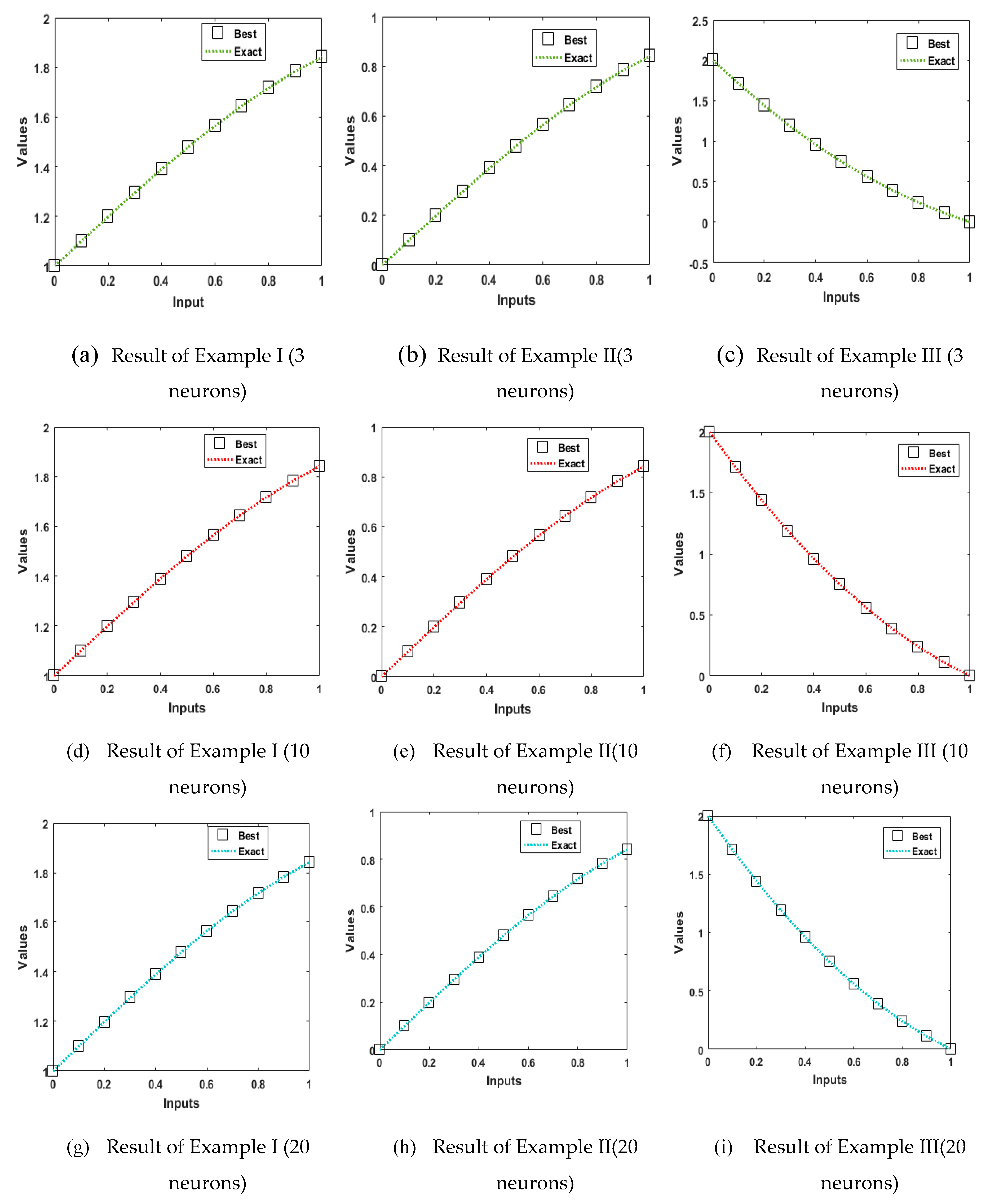
For the comparison, the obtained outcomes have been compared with the exact solutions to solve each example of the PDM using 3, 10 and 20 number of neurons. These comparison plots are drawn in Figure 3 andone can observe that the optimal results are intersected with the exact outcomes for each example of the PDM by considering 3, 10 and 20 number of neurons, which shows the precision of MWNN-GAIPAS.
The performances through statics of the designed MWNN-GAAPAS for each example of PDM using 3, 10 and 20 numbers of neurons is tabulated in Table 2, Table 3 and Table 4, respectively. The Minimum (Min), Median (Med), Mean, S.I.R and standard deviation (SD) value for Examples I, II and III found in good measures for each Example of the PDM. These very small calculated values based on these statistics gages for each example of the PDM based 3, 10 and 20 neurons shows the accurateness of designed MWNN-GAIPAS.
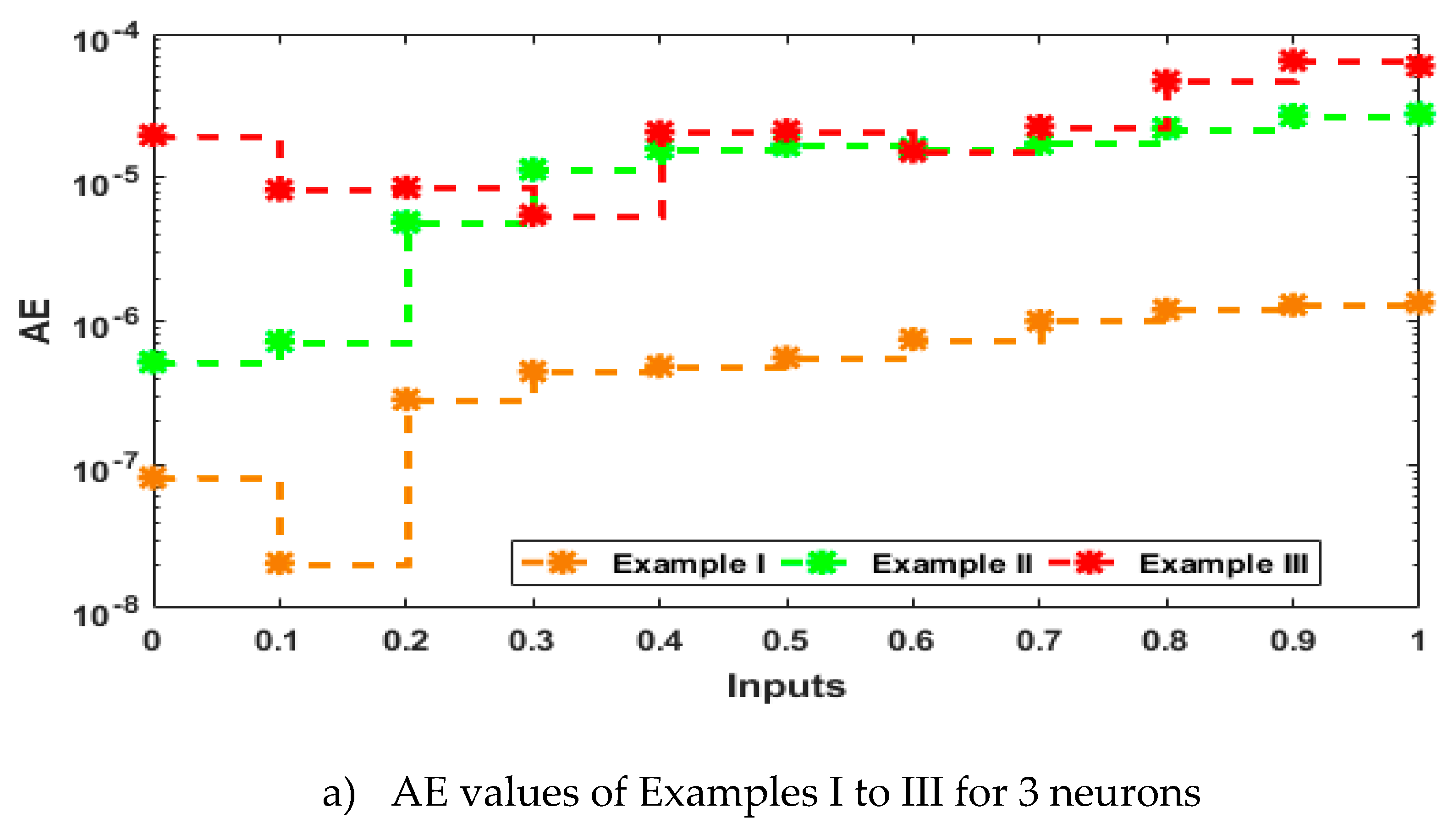
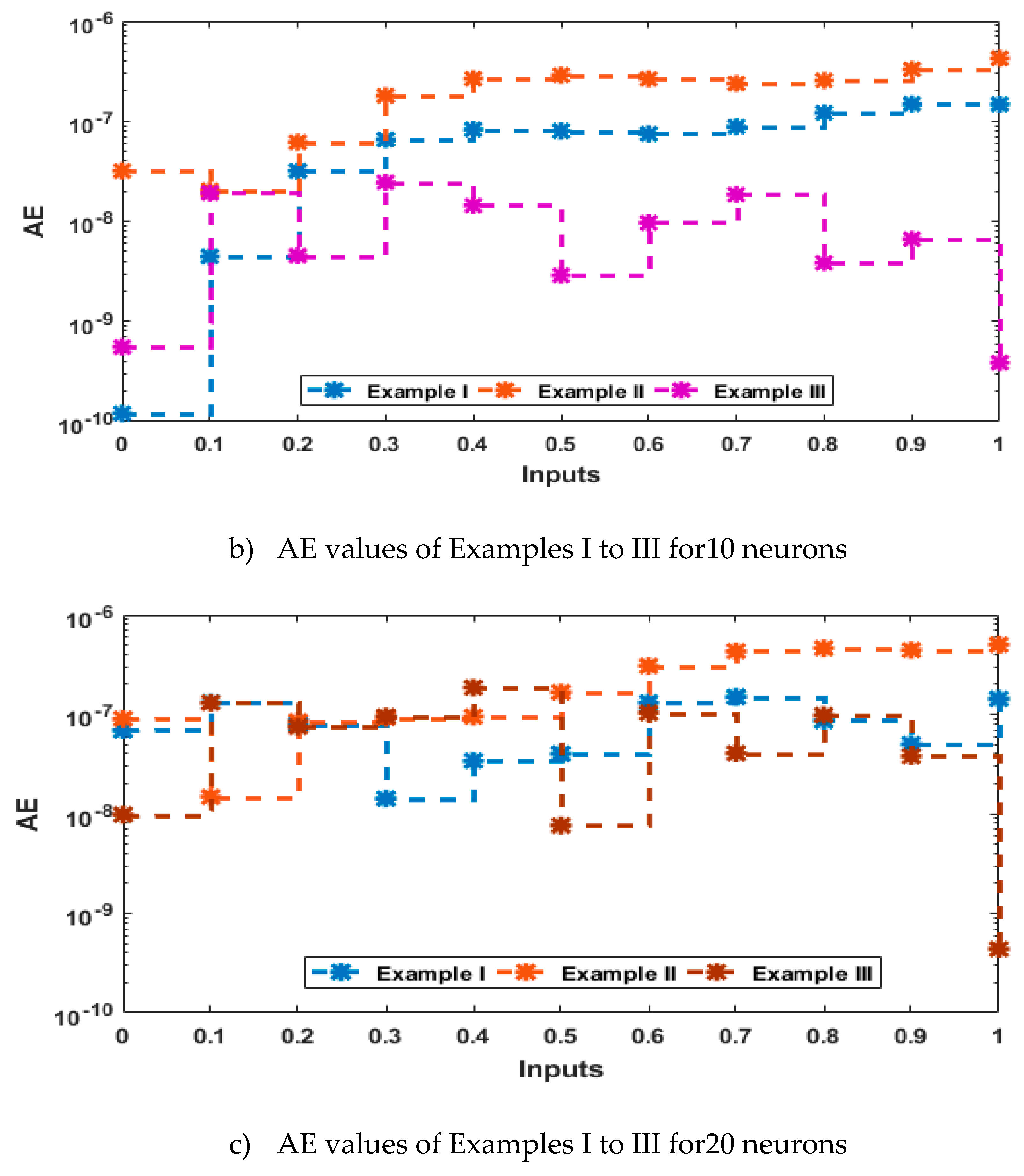
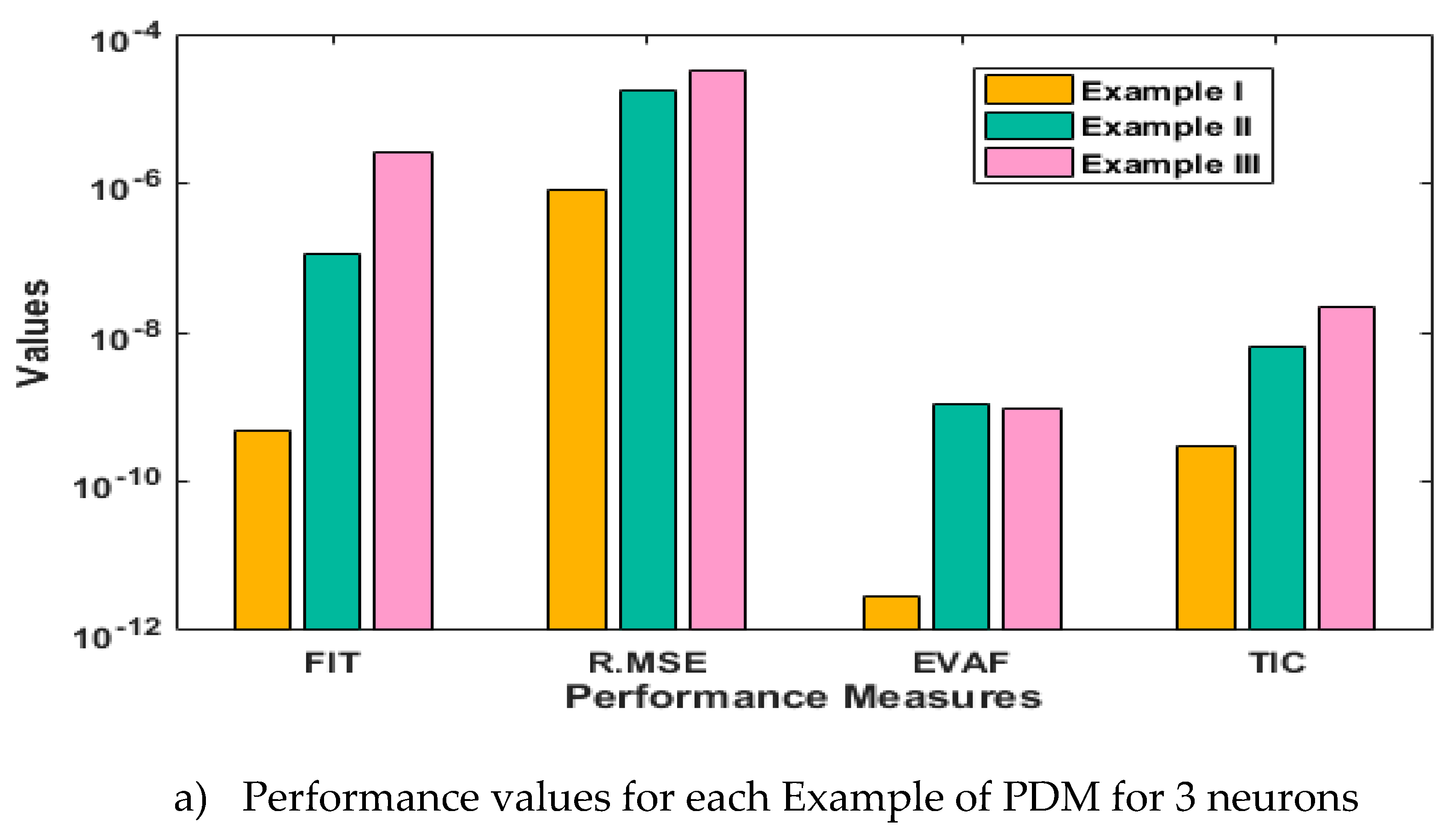
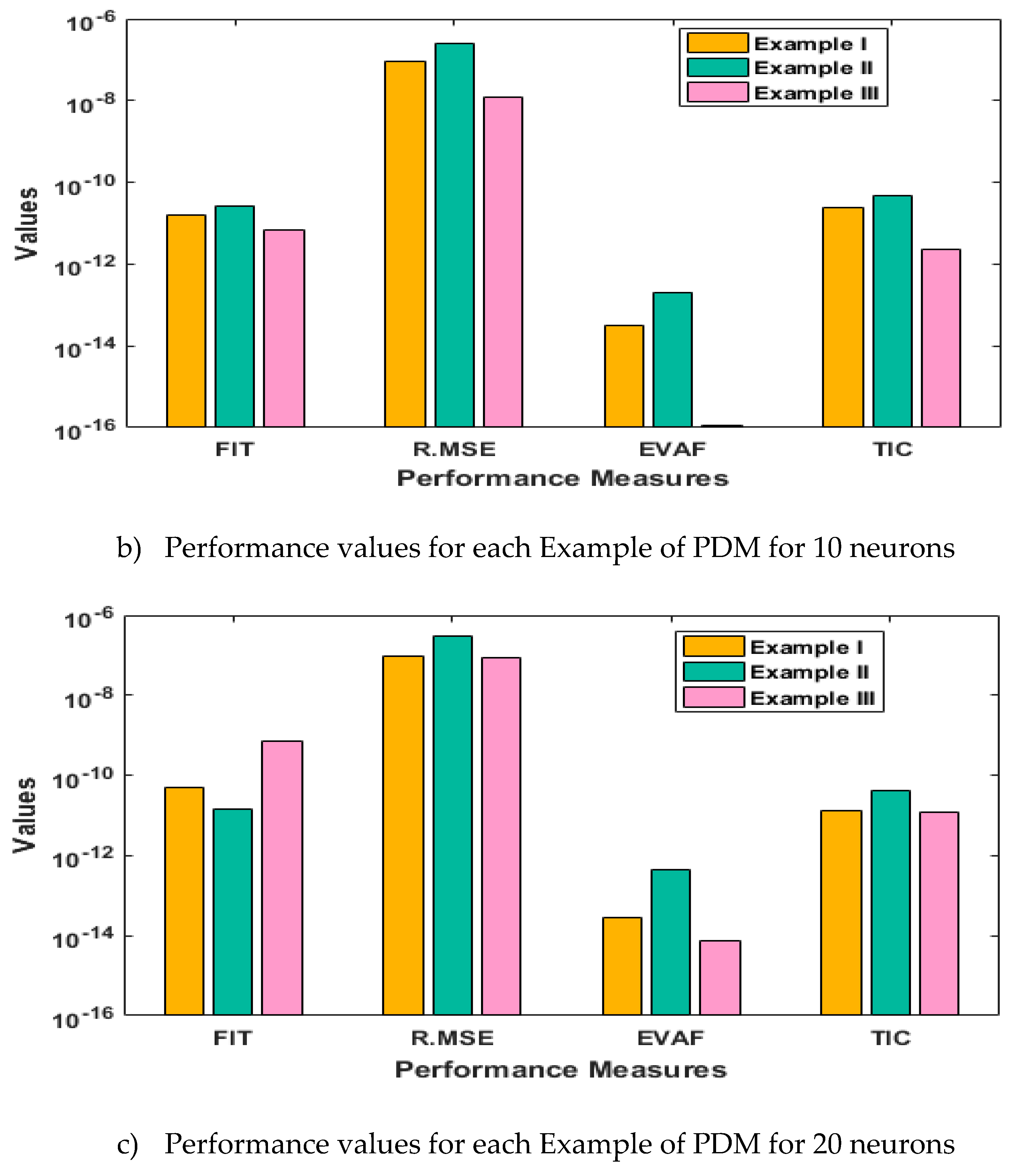
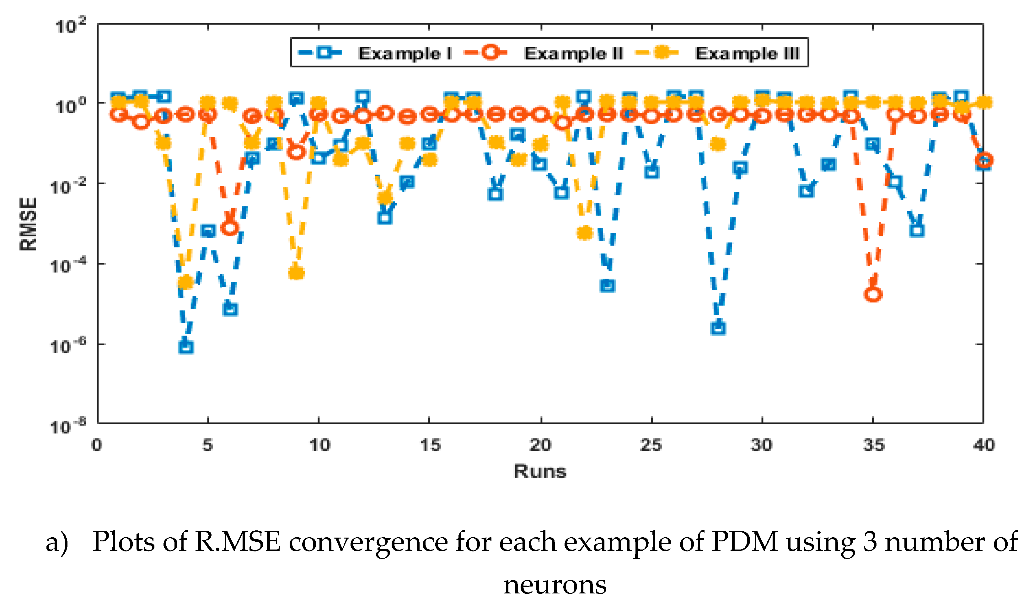
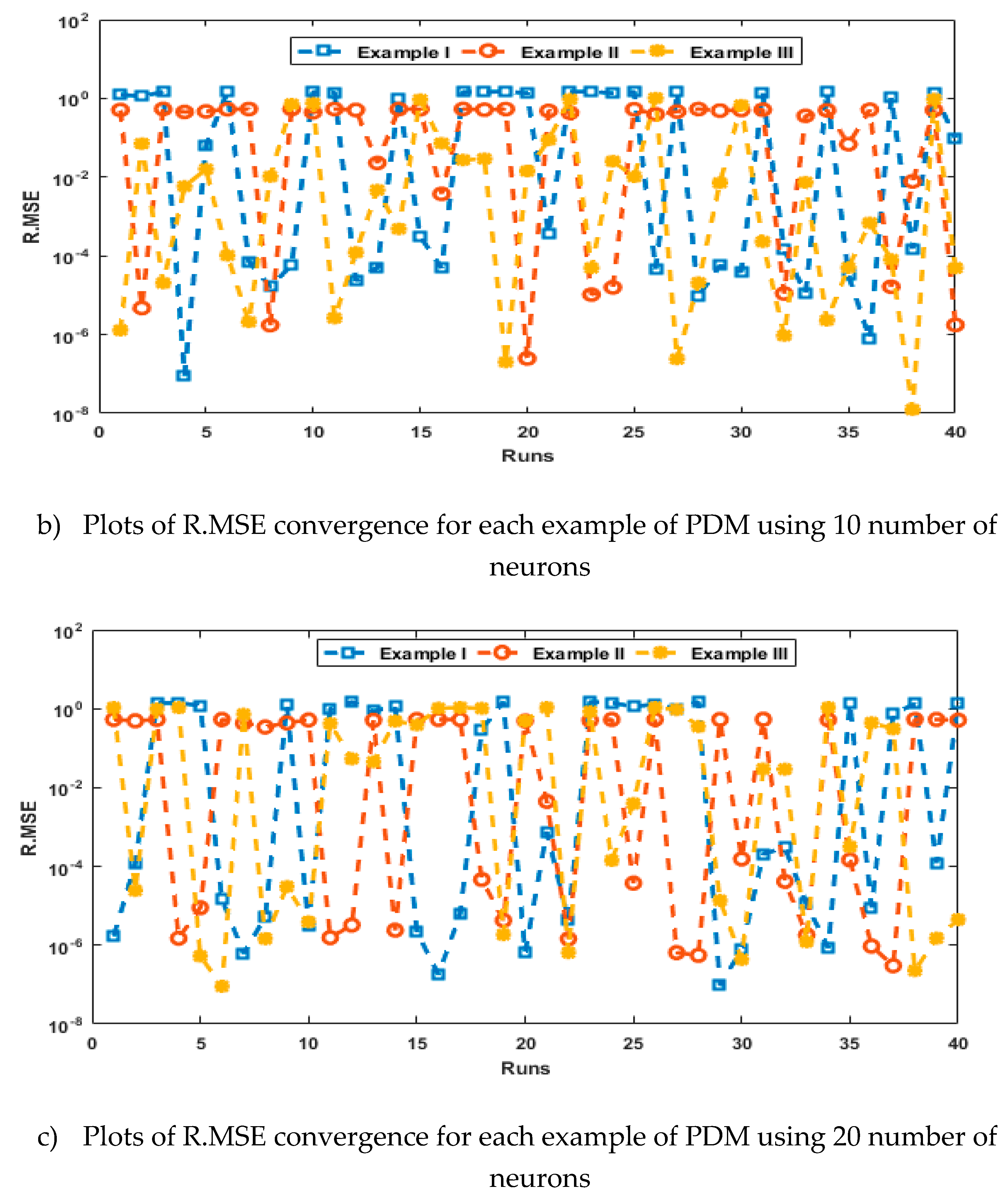
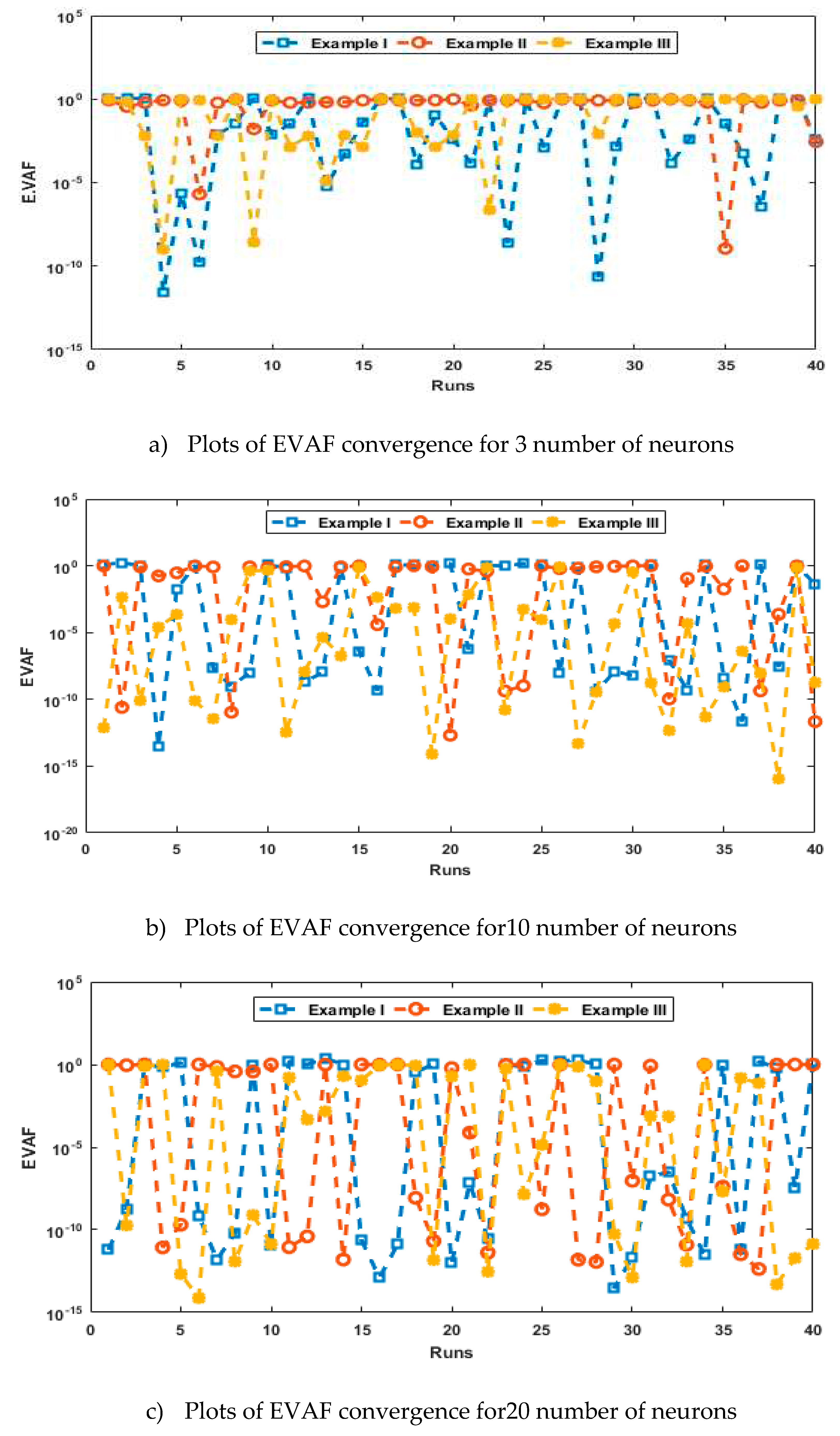
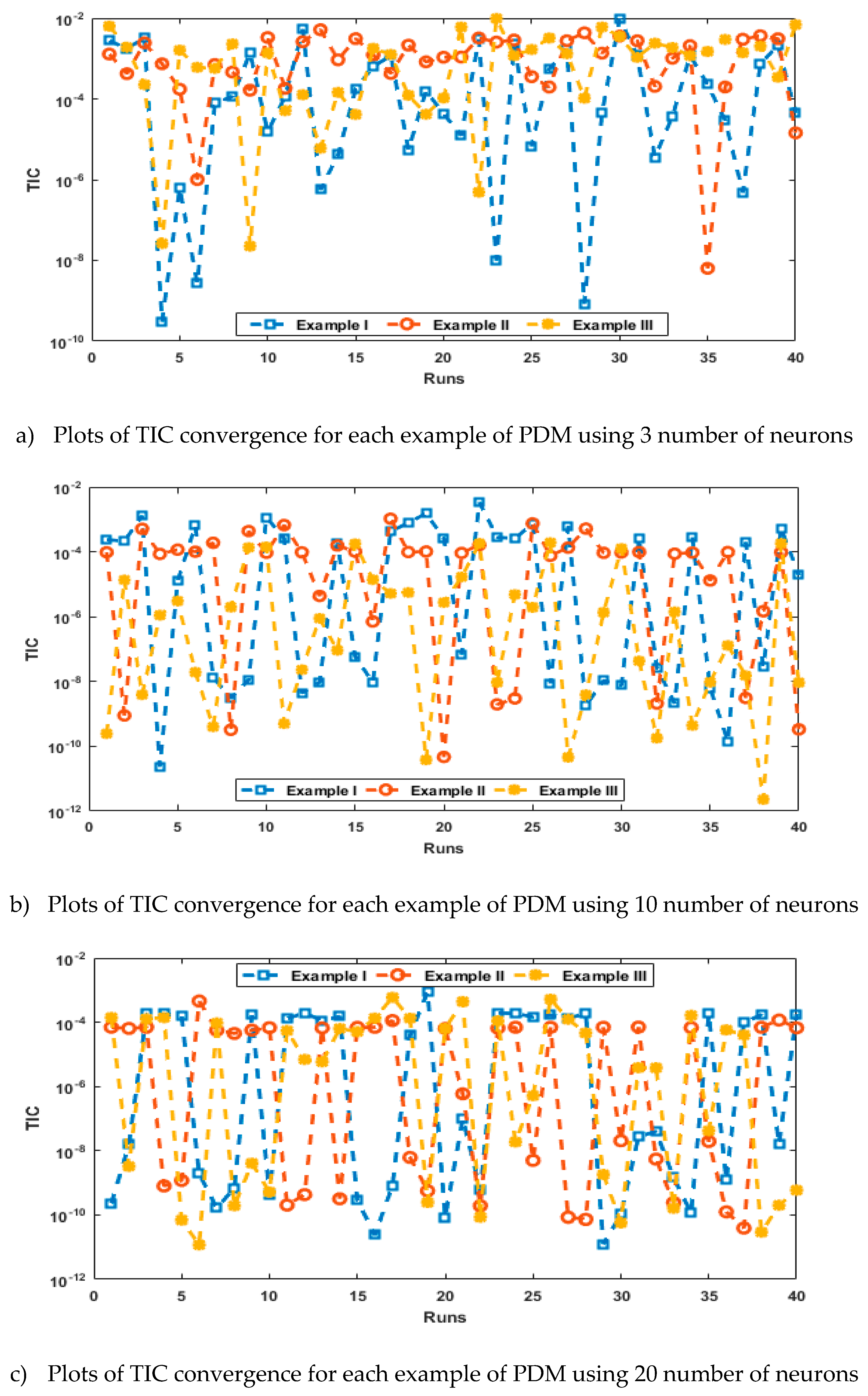
The plots of absolute error (AE) for each example of the PDM for 3, 10 and 20 number of neurons are shown in Figure 4(a), 4(b) and 4(c), respectively. One can observe that the AE values using 3 numbers of neurons for examples 1, 2 and 3 lie 10-7- 10-9, 10-5- 10-6and 10-4 - 10-6.The AE for 10 neurons for examples 1, 2 and 3 lie 10-7- 10-9, 10-6- 10-8 and 10-07- 10-9. For 20 neurons, the AE lies around for examples 1, 2 and 3 lie around 10-07 - 10-09, 10-6- 10-07 and 10-07- 10-10, respectively. It is clear in the AE for each example of the PDM are found in good ranges for considering 3,10 and 20 numbers of neurons. The R.MSE, Fitness (FIT), TIC and EVAF are measured in Figure 5a–c for 3, 10 and 20 number of neurons. Figure 5(a) presentsthat the best FIT for Examples I to IIIis calculated as10-09- 10-10, 10-07- 10-09 and 10-5- 10-6, respectively. Theoptimal R.MSE is found around 10-6 to 10-07, while the R.MSE for other two Examples lie around 10-5 to 10-6.The best EVAF values are found around 10-11 to 10-12, while the R.MSE for other two Examples lie around 10-09 to 10-10. The TIC best values for all the Examples based on 3 neurons are calculated around 10-09 to 10-10. The performance based on 10 neurons is presented in Figure 5(b). The plots in this figure indicate the FIT and EVAF best measures for each example of the PDM lie 10-10 to 10-12, while the R.MSE and TIC best values lie around 10-6 to 10-8 and 10-10 to 10-12, respectively. The performance based on 20 numbers of neurons is presented in Figure 5(c). The plots in this figure indicate that the best values of these statistical operators for example I to III lie around 10-10- 10-12, 10-6- 10-8, 10-12- 10-14 and 10-10- 10-12.These obtained outcomes verify the competent trend for solving PDM based on 3, 10 and 20 numbers of neurons.
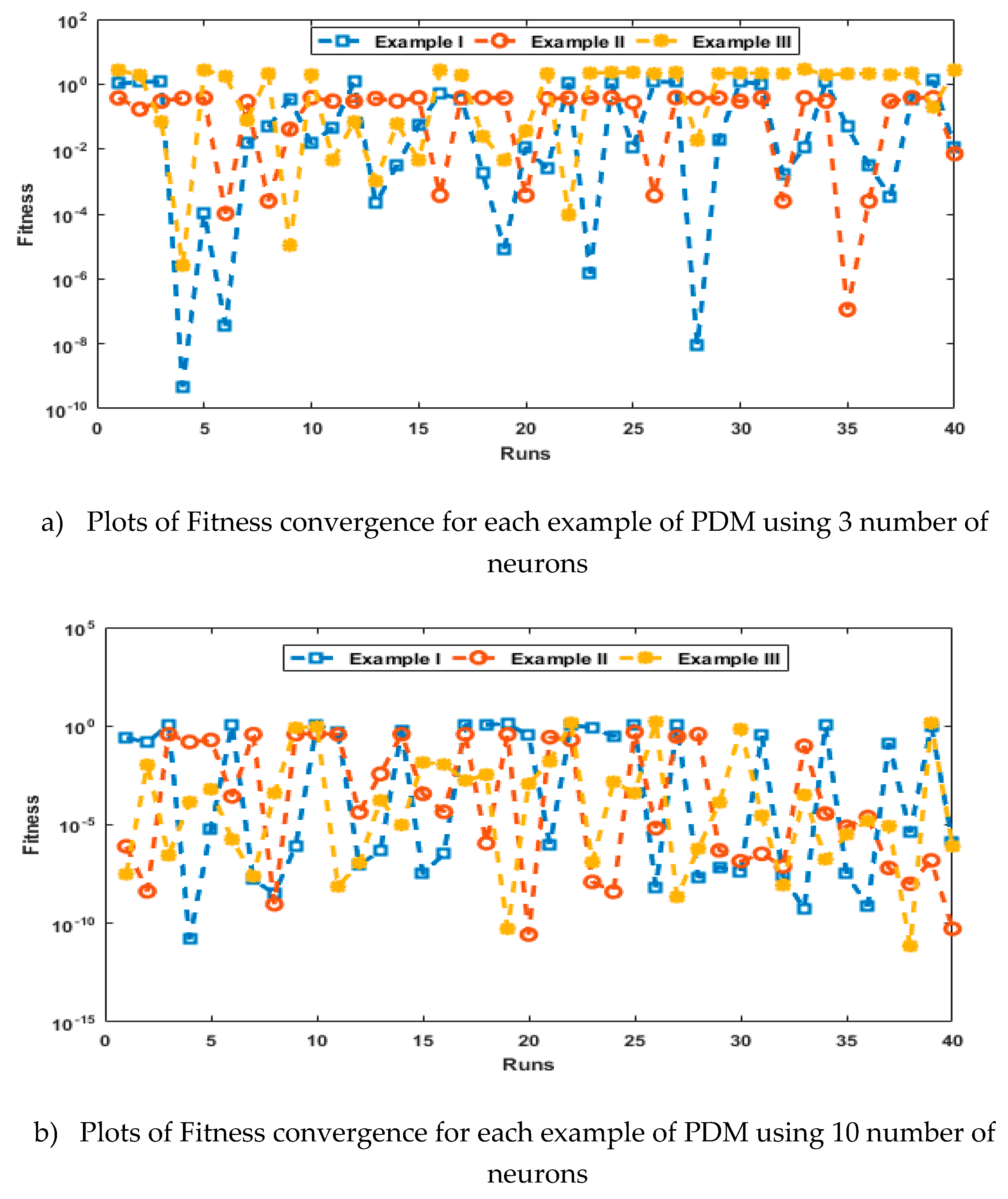
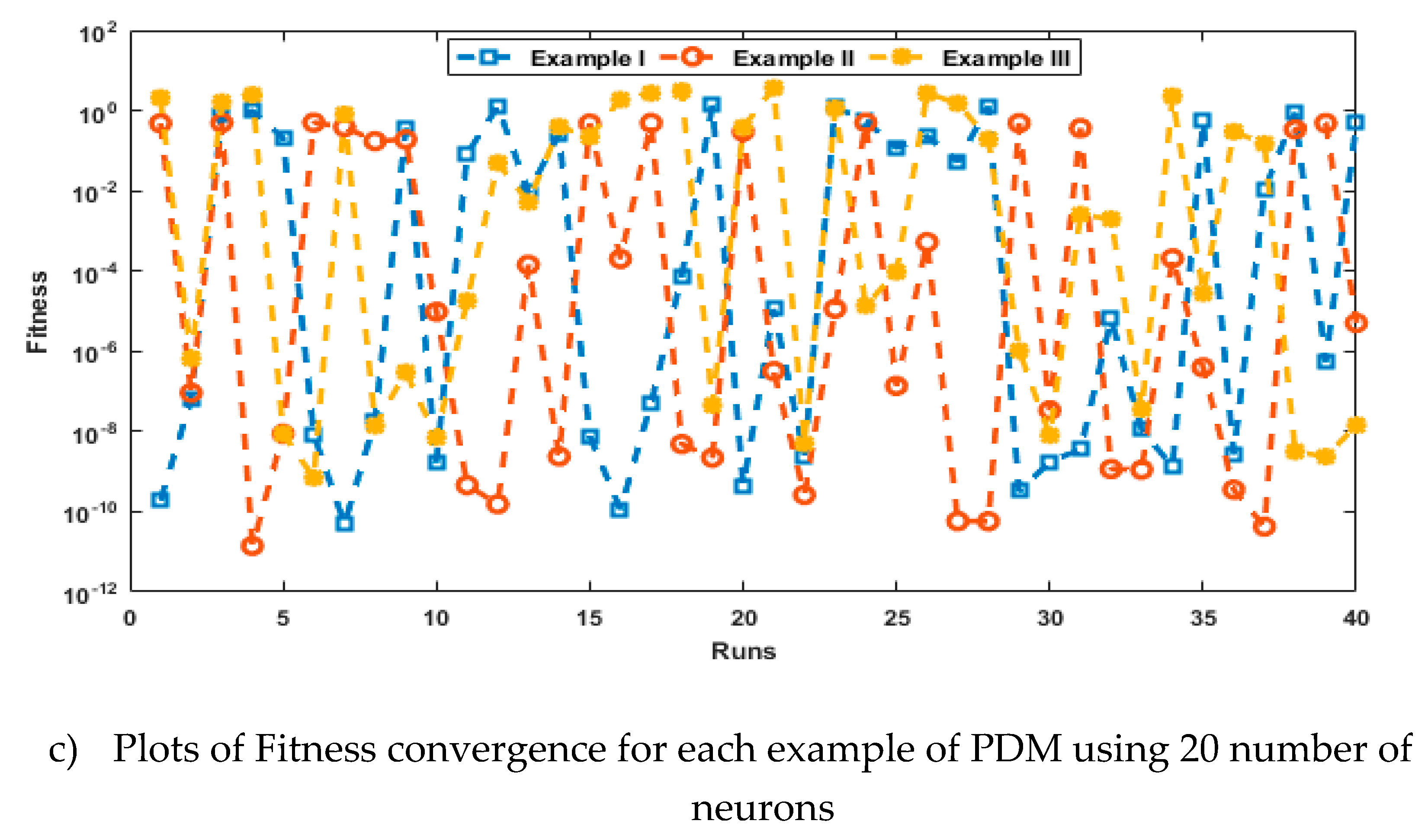
The performances-based statics to solve each example of PDM are drawn in Figure 6, Figure 7, Figure 8 and Figure 9 for 3, 10 and 20 number of neurons. Figure 6 presents the FIT measures for forty trials to present the solutions of each Example of PDM using 3, 10 and 20 numbers of neurons. One can observe that the best runs are found around 10-01to 10-04, 10-02 to 10-8 and 10-02to 10-12 for solving each Example of the PDM using 3, 10 and 20 number of neurons. Figure 7 shows the statistical investigations through R.MSE using MWNN-GAIPAS for each example of the PDM taking 3, 10 and 20 number of neurons. It is seen that the best runs are found around 10-01 to 10-3, 10-02to 10-6 and 10-02to 10-8 for solving each Example of the PDM using 3, 10 and 20 numbers of neurons. Figure 8 shows the statistical investigations through EVAF using MWNN-GAIPAS for each example of the PDM taking 3, 10 and 20 number of neurons. It is seen that the best runs are found around 10-01to 10-5, 10-02to 10-08 and 10-02to 10-15 for solving each Example of the PDM using 3, 10 and 20 numbers of neurons. Figure 9 represents the statistical investigations through TIC using MWNN-GAIPAS for each example of the PDM taking 3, 10 and 20 number of neurons. It is seen that the best runs are found around 10-02to 10-07, 10-04to 10-10 and 10-04to 10-12 for solving each Example of the PDM using 3, 10 and 20 numbers of neurons. It is easy in understanding that by taking three numbers of neurons, the method performs quicker in the comparison of 10 and 20 numbers of neurons, but one can get more reliable solutions by taking a larger neuron.
The statistical performances through MWNN-GAIPAS for each example of PDM for forty independent executions using 3, 10 and 20 numbers of neurons are provided in Table 5, Table 6 and Table 7, respectively. The smaller optimum measures of the statistical operators further validate the exactitude of the MWNN-GAIPAS.

5. Conclusion

The design of Morlet wavelet neural network using the hybridization process of global and local search schemes GA-IPAS are presented to solve the prediction model. This model is a kind of functional differential equation that work as an opposite of the historical delay differential models. The analysis of neurons for 3, 10 and 20 number of neurons is also presented to solve three different examples of the prediction differential model. The overlapping of the obtained results through the proposed methodology with the exact results shows the exactness of each example of the model based on3, 10 and 20 neurons. The AE for examples I to III is found in good measures for 3, 10 and 20 number of neurons. One can access that the proposed MWNN-GAIPAS can be implemented accurately, efficiently and viably for different number of neurons to solve the model. Furthermore, statistical soundings based on forty runs for solving the prediction system in terms of statistical Min, Med, standard deviation, mean and SI. Range operators, which authenticates the accurateness, and trust worthiness of MWNN-GAIPAS that is updated further by the investigations of TIC, EVAF and R.MSE along with their global presentations to solve each example of the prediction differential system. It is also noticed that the small optimum values of these operators further used to justify the accuracy and precision of MWNN-GAIPAS.
In upcoming studies, the MWNN-GAIPAS can be executed to solve the biological systems, fluid dynamic nonlinear equations and higher order singular differential models [47,48,49,50,51].

Funding

This work was supported and funded by the Deanship of Scientific Research at Imam Mohammad Ibn Saud Islamic University (IMSIU) (grant number IMSIU-RP23088).

Conflicts of Interest

The authors declare that they have no conflict of interest.

References

  1. Niculescu, S.I., 2001. Delay effects on stability: a robust control approach (Vol. 269). Springer Science & Business Media.
  2. Zulqurnain Sabir et al., 2021, Design of neuro-swarming heuristic solverfor multi-pantograph singular delay differential equation, Fractals. [CrossRef]
  3. Guirao, J.L. et al. 2020. Design and numerical solutions of a novel third-order nonlinear Emden–Fowler delay differential model. Mathematical Problems in Engineering, 2020.
  4. Sabir, Z. et al, 2021. Solving a novel designed second order nonlinear Lane-Emden delay differential model using the heuristic techniques. Applied Soft Computing, p.107105.
  5. Abdelkawy, M.A. et al., 2020. Numerical investigations of a new singular second-order nonlinear coupled functional Lane–Emden model. Open Physics, 18(1), pp.770-778.
  6. Bildik, N. and Deniz, S., 2017. A new efficient method for solving delay differential equations and a comparison with other methods. The European Physical Journal Plus, 132(1), pp.1-11.
  7. Rahimkhani, P., Ordokhani, Y. and Babolian, E., 2017. A new operational matrix based on Bernoulli wavelets for solving fractional delay differential equations. Numerical Algorithms, 74(1), pp.223-245.
  8. Sabir, Z. et al., 2020. On a new model based on third-order nonlinear multisingular functional differential equations. Mathematical Problems in Engineering, 2020.
  9. Aziz, I. and Amin, R., 2016. Numerical solution of a class of delay differential and delay partial differential equations via Haar wavelet. Applied Mathematical Modelling, 40(23-24), pp.10286-10299.
  10. Frazier, M.W., 1999. Background: Complex Numbers and Linear Algebra. An Introduction to Wavelets through Linear Algebra, pp.7-100.
  11. Tomasiello, S., 2017. An alternative use of fuzzy transform with application to a class of delay differential equations. International Journal of Computer Mathematics, 94(9), pp.1719-1726.
  12. Vaid, M.K. and Arora, G., 2019. Solution of second order singular perturbed delay differential equation using trigonometric B-spline. International Journal of Mathematical, Engineering and Management Sciences, 4(2), pp.349-360.
  13. Hashemi, M.S., Atangana, A. and Hajikhah, S., 2020. Solving fractional pantograph delay equations by an effective computational method. Mathematics and Computers in Simulation, 177, pp.295-305.
  14. Adel, W. and Sabir, Z., 2020. Solving a new design of nonlinear second-order Lane–Emden pantograph delay differential model via Bernoulli collocation method. The European Physical Journal Plus, 135(6), p.427.
  15. Erdogan, F et al., 2020. A finite difference method on layer-adapted mesh for singularly perturbed delay differential equations. Applied Mathematics and Nonlinear Sciences, 5(1), pp.425-436.
  16. Seong, H.Y. and Majid, Z.A., 2017. Solving second order delay differential equations using direct two-point block method. Ain Shams Engineering Journal, 8(1), pp.59-66.
  17. Sabir, Z. et al, 2020,. Design of a novel second order prediction differential model and solved by using Adams and explicit Runge-Kutta numerical methods. Volume 2020 Article ID 9704968 . [CrossRef]
  18. Sabir, Z., et al., 2020. Integrated neuro-evolution heuristic with sequential quadratic programming for second-order prediction differential models. Numerical Methods for Partial Differential Equations.
  19. Umar, M., Amin, F., Wahab, H.A. and Baleanu, D., 2019. Unsupervised constrained neural network modeling of boundary value corneal model for eye surgery. Applied Soft Computing, 85, p.105826.
  20. Raja, M.A.Z. et al, 2019. Numerical solution of doubly singular nonlinear systems using neural networks-based integrated intelligent computing. Neural Computing and Applications, 31(3), pp.793-812.
  21. Sabir, Z., et al, 2020. Intelligence computing approach for solving second order system of Emden–Fowler model. Journal of Intelligent & Fuzzy Systems, pp.1-16.
  22. Umar, M. et al., 2020. A stochastic numerical computing heuristic of SIR nonlinear model based on dengue fever. Results in Physics, 19, p.103585.
  23. Sabir, Z. et al., 2019. Stochastic numerical approach for solving second order nonlinear singular functional differential equation. Applied Mathematics and Computation, 363, p.124605.
  24. Sabir, Z. et al., 2020. Neuro-swarm intelligent computing to solve the second-order singular functional differential model. The European Physical Journal Plus, 135(6), p.474.
  25. Umar, M., et al., 2020. Stochastic numerical technique for solving HIV infection model of CD4+ T cells. The European Physical Journal Plus, 135(6), p.403.
  26. Sabir, Z., et al,. 2018. Neuro-heuristics for nonlinear singular Thomas-Fermi systems. Applied Soft Computing, 65, pp.152-169.
  27. Umar, M., et al., 2019. Intelligent computing for numerical treatment of nonlinear prey–predator models. Applied Soft Computing, 80, pp.506-524.
  28. Raja, M.A.Z et al., 2015. Design of stochastic solvers based on genetic algorithms for solving nonlinear equations. Neural Computing and Applications, 26(1), pp.1-23.
  29. Zulqurnain Sabir et al., Design of neuro-swarming heuristic solverfor multi-pantograph singular delay differential equation, Fractals. [CrossRef]
  30. Sabir, Z. et al., 2020. FMNEICS: fractional Meyer neuro-evolution-based intelligent computing solver for doubly singular multi-fractional order Lane–Emden system. Computational and Applied Mathematics, 39(4), pp.1-18.
  31. Raja, M.A.Z. et al., 2018. A new stochastic computing paradigm for the dynamics of nonlinear singular heat conduction model of the human head. The European Physical Journal Plus, 133(9), p.364.
  32. Sabir, Z. et al., 2020. Design of neuro-swarming-based heuristics to solve the third-order nonlinear multi-singular Emden–Fowler equation. The European Physical Journal Plus, 135(6), p.410.
  33. Sabir, Z. et al., 2020. Novel design of Morlet wavelet neural network for solving second order Lane–Emden equation. Mathematics and Computers in Simulation, 172, pp.1-14.
  34. Reddy, G.T., Reddy, M.P.K., Lakshmanna, K., Rajput, D.S., Kaluri, R. and Srivastava, G., 2020. Hybrid genetic algorithm and a fuzzy logic classifier for heart disease diagnosis. Evolutionary Intelligence, 13(2), pp.185-196.
  35. Mayer, M.J., Szilágyi, A. and Gróf, G., 2020. Environmental and economic multi-objective optimization of a household level hybrid renewable energy system by genetic algorithm. Applied Energy, 269, p.115058.
  36. Zou, D., Li, S., Kong, X., Ouyang, H. and Li, Z., 2019. Solving the combined heat and power economic dispatch problems by an improved genetic algorithm and a new constraint handling strategy. Applied energy, 237, pp.646-670.
  37. Sabir, Z. et al., 2020. Heuristic computing technique for numerical solutions of nonlinear fourth order Emden–Fowler equation. Mathematics and Computers in Simulation, 178, pp.534-548.
  38. Armaghani, D.J., Hasanipanah, M., Mahdiyar, A., Majid, M.Z.A., Amnieh, H.B. and Tahir, M.M., 2018. Airblast prediction through a hybrid genetic algorithm-ANN model. Neural Computing and Applications, 29(9), pp.619-629.
  39. Umar, M. et al., 2020. A Stochastic Intelligent Computing with Neuro-Evolution Heuristics for Nonlinear SITR System of Novel COVID-19 Dynamics. Symmetry, 12(10), p.1628.
  40. Sabir, Z. et al., 2020. Design of stochastic numerical solver for the solution of singular three-point second-order boundary value problems. Neural Computing and Applications, pp.1-17.
  41. Jiang, Y., Wu, P., Zeng, J., Zhang, Y., Zhang, Y. and Wang, S., 2020. Multi-parameter and multi-objective optimisation of articulated monorail vehicle system dynamics using genetic algorithm. Vehicle System Dynamics, 58(1), pp.74-91.
  42. Bertocchi, C., Chouzenoux, E., Corbineau, M.C., Pesquet, J.C. and Prato, M., 2020. Deep unfolding of a proximal interior point method for image restoration. Inverse Problems, 36(3), p.034005.
  43. Wright, S.E. and Lim, S., 2020. Solving nested-constraint resource allocation problems with an interior point method. Operations Research Letters, 48(3), pp.297-303.
  44. Pesteh, S., Moayyed, H. and Miranda, V., 2020. Favorable properties of interior point method and generalized correntropy in power system state estimation. Electric Power Systems Research, 178, p.106035.
  45. Garreis, S., Surowiec, T.M. and Ulbrich, M., 2021. An interior-point approach for solving risk-averse PDE-constrained optimization problems with coherent risk measures. SIAM Journal on Optimization, 31(1), pp.1-29.
  46. Asadi, S., Darvay, Z., Lesaja, G., Mahdavi-Amiri, N. and Potra, F., 2020. A Full-Newton Step Interior-Point Method for Monotone Weighted Linear Complementarity Problems. Journal of Optimization Theory and Applications, 186(3), pp.864-878.
  47. Sanchez, Y.G. et al. 2020. Design of a nonlinear SITR fractal model based on the dynamics of a novel coronavirus (COVID). Fractals, 28, p.2040026.
  48. Guerrero Sánchez, Y. et al., 2020. Analytical and approximate solutions of a novel nervous stomach mathematical model. Discrete Dynamics in Nature and Society, 2020.
  49. Sabir, Z., Sakar, M.G., Yeskindirova, M. and Saldir, O., 2020. Numerical investigations to design a novel model based on the fifth order system of Emden–Fowler equations. Theoretical and Applied Mechanics Letters, 10(5), pp.333-342.
  50. Sajid, T. et al,. 2020. Upshot of radiative rotating Prandtl fluid flow over a slippery surface embedded with variable species diffusivity and multiple convective boundary conditions. Heat Transfer.
  51. Umar, M. et al., 2020. The 3-D flow of Casson nanofluid over a stretched sheet with chemical reactions, velocity slip, thermal radiation and Brownian motion. Thermal Science, 24(5 Part A), pp.2929-2939.
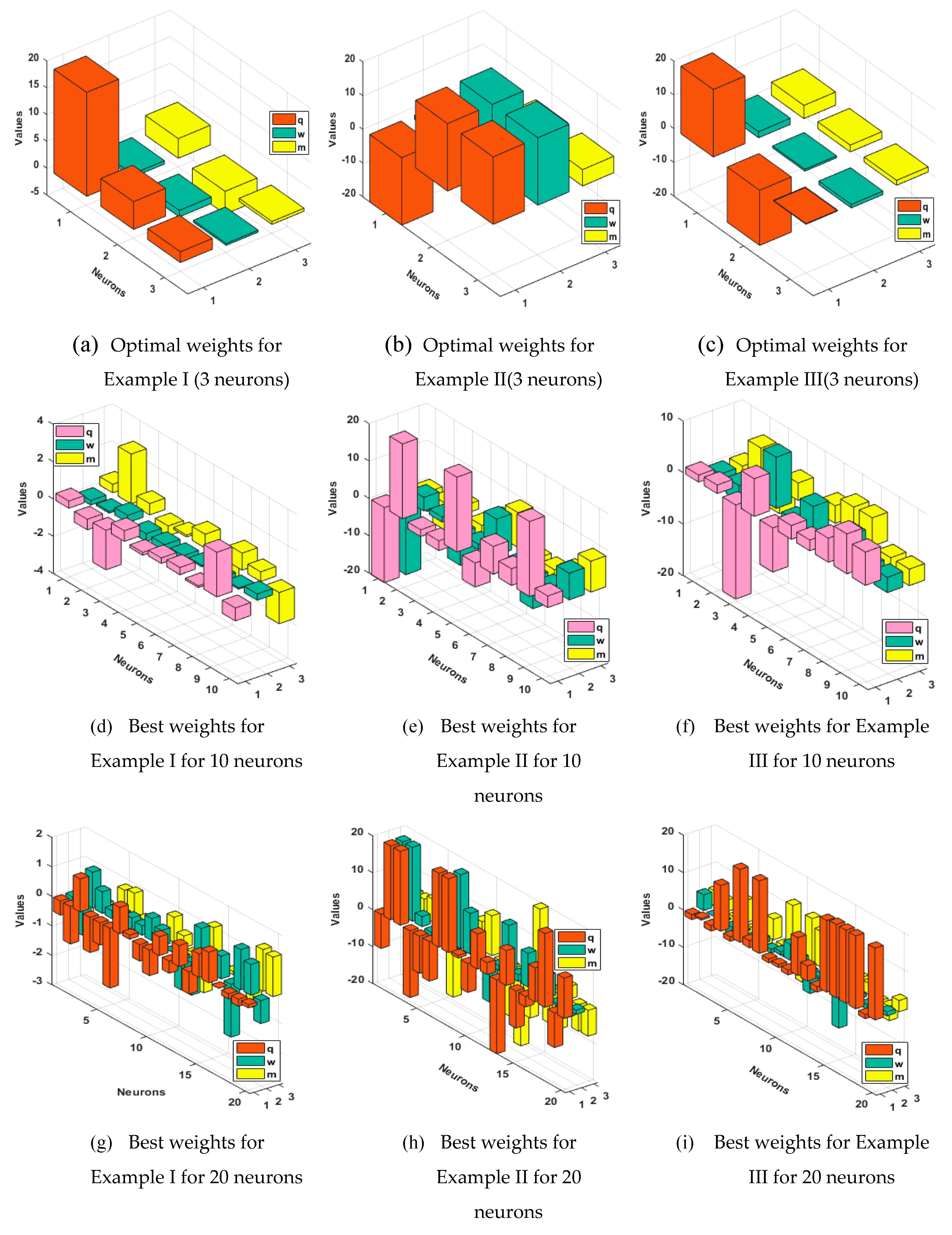
Figure 2. Best weights of MWNN-GAIPAS for each example of the PDM using 3, 10 and 20 number of neurons.
Preprints 86981 g002
Figure 3. Comparison of the best and exact solutions based MWNN-GAIPAS for solving each example of the PDM using 3, 10 and 20 number of neurons.
Preprints 86981 g003
Figure 4. AE for solving each example of PDM using 3, 10 and 20 neurons.
Preprints 86981 g004aPreprints 86981 g004b
Figure 5. Performance values for solving each example of the PDM based 3, 10 and 20 neurons.
Preprints 86981 g005aPreprints 86981 g005b
Figure 6. Statistical investigations-based fitness for example I to III by taking 3, 10 and 20 number of neurons.
Preprints 86981 g006aPreprints 86981 g006b
Figure 7. Statistical investigations of R.MSE for example I to III by taking 3, 10 and 20 number of neurons.
Preprints 86981 g007aPreprints 86981 g007b
Figure 8. Statistical investigations of EVAF for each example by taking 3, 10 and 20 number of neurons.
Preprints 86981 g008
Figure 9. Statistical investigations based TIC operator for example I to III by taking 3, 10 and 20 number of neurons.
Preprints 86981 g009
Table 1. The optimization based MWNN-GAIPAS is given in the pseudo code for solving the PDM.
Preprints 86981 i001
Preprints 86981 i002
Table 2. Statistical measures using MWNN-GAAPAS for each example of PDM using 3 neurons.
Mode y ^ ( t )
0 0.1 0.2 0.3 0.4 0.5 0.6 0.7 0.8 0.9 1
E-I Min 4.14E-9 2.07E-8 2.85E-7 4.46E-7 4.86E-7 5.58E-7 7.48E-7 1.00E-6 1.20E-6 1.30E-6 1.34E-6
Mean 3.75E-1 4.13E-1 4.54E-1 4.98E-1 5.41E-1 5.83E-1 6.22E-1 6.59E-1 6.92E-1 7.23E-1 7.49E-1
SD 4.46E-1 5.1E-1 5.57E-1 6.7E-1 6.53E-1 6.95E-1 7.35E-1 7.72E-1 8.05E-1 8.34E-1 8.60E-1
Med 3.93E-2 2.13E-2 1.21E-2 2.48E-2 4.61E-2 6.65E-2 8.59E-2 1.05E-1 1.23E-1 1.41E-1 1.59E-1
S.IR 4.38E-1 4.84E-1 5.38E-1 5.88E-1 6.35E-1 6.79E-1 7.21E-1 7.60E-1 7.97E-1 8.30E-1 8.59E-1
E-II Min 5.20E-7 7.23E-7 4.89E-6 1.14E-5 1.59E-5 1.68E-5 1.60E-5 1.72E-5 2.20E-5 2.71E-5 2.77E-5
Mean 6.72E-2 1.31E-1 2.03E-1 2.76E-1 3.50E-1 4.22E-1 4.91E-1 5.57E-1 6.18E-1 6.74E-1 7.23E-1
SD 3.19E-2 5.19E-2 7.16E-2 9.52E-2 1.19E-1 1.43E-1 1.66E-1 1.89E-1 2.10E-1 2.29E-1 2.46E-1
Med 7.70E-2 1.57E-1 2.33E-1 3.6E-1 3.89E-1 4.79E-1 5.65E-1 6.44E-1 7.17E-1 7.83E-1 8.41E-1
S.IR 1.55E-2 2.86E-2 1.99E-2 1.31E-2 1.46E-2 2.09E-2 2.71E-2 3.30E-2 3.83E-2 4.31E-2 4.70E-2
E-III Min 1.98E-5 8.21E-6 8.50E-6 5.50E-6 7.92E-6 2.12E-5 1.52E-5 1.19E-5 2.95E-5 5.74E-5 5.59E-5
Mean 1.25E-1 1.08E-1 9.21E-1 7.77E-1 6.43E-1 5.19E-1 4.03E-1 2.95E-1 1.90E-1 1.28E-1 1.50E-1
SD 9.57E-1 8.20E-1 6.93E-1 5.72E-1 4.60E-1 3.60E-1 2.75E-1 2.15E-1 1.98E-1 2.18E-1 1.06E-1
Med 1.91E-1 1.65E-1 1.40E-1 1.17E-1 9.51E-1 7.42E-1 5.37E-1 3.29E-1 1.37E-1 8.53E-2 1.65E-1
S.IR 9.91E-1 8.47E-1 7.10E-1 5.77E-1 4.52E-1 3.39E-1 2.31E-1 1.34E-1 5.59E-2 6.92E-2 7.89E-2
Table 3. The performances through statics of MWNN-GAAPAS for each example of PDM using 10 neurons.
Mode y ^ ( t )
0 0.1 0.2 0.3 0.4 0.5 0.6 0.7 0.8 0.9 1
E-I Min 1.20E-9 4.45E-9 3.18E-8 6.57E-8 8.26E-8 7.97E-8 7.48E-8 8.81E-8 1.21E-7 1.48E-7 1.47E-7
Mean 4.26E-1 4.78E-1 5.34E-1 5.88E-1 6.39E-1 6.88E-1 7.33E-1 7.75E-1 8.14E-1 8.48E-1 8.79E-1
SD 4.46E-1 4.97E-1 5.50E-1 6.02E-1 6.51E-1 6.98E-1 7.42E-1 7.83E-1 8.20E-1 8.54E-1 8.83E-1
Med 2.54E-1 2.99E-1 3.68E-1 4.31E-1 4.80E-1 5.27E-1 5.71E-1 6.13E-1 6.53E-1 6.89E-1 7.22E-1
S.IR 4.66E-1 5.23E-1 5.79E-1 6.33E-1 6.82E-1 7.27E-1 7.68E-1 8.06E-1 8.40E-1 8.77E-1 9.05E-1
E-II Min 1.15E-8 2.04E-8 6.16E-8 1.79E-7 2.65E-7 2.88E-7 2.64E-7 2.38E-7 2.55E-7 3.30E-7 4.24E-7
Mean 4.16E-2 8.85E-2 1.47E-1 2.06E-1 2.63E-1 3.19E-1 3.72E-1 4.23E-1 4.70E-1 5.12E-1 5.48E-1
SD 6.10E-2 7.67E-2 1.03E-1 1.36E-1 1.73E-1 2.10E-1 2.46E-1 2.79E-1 3.11E-1 3.40E-1 3.64E-1
Med 2.32E-3 7.26E-2 1.73E-1 2.69E-1 3.58E-1 4.48E-1 5.15E-1 5.86E-1 6.52E-1 7.12E-1 7.61E-1
S.IR 3.70E-2 7.45E-2 1.11E-1 1.50E-1 1.93E-1 2.36E-1 2.79E-1 3.18E-1 3.53E-1 3.84E-1 4.08E-1
E-III Min 5.56E-9 1.91E-8 4.54E-9 2.45E-8 1.44E-8 2.28E-9 9.65E-9 1.85E-8 3.85E-9 6.66E-9 3.87E-9
Mean 2.30E-1 2.50E-1 2.13E-1 1.80E-1 1.50E-1 1.24E-1 9.84E-2 7.42E-2 5.08E-2 2.80E-2 3.14E-2
SD 5.50E-1 5.48E-1 4.69E-1 3.97E-1 3.28E-1 2.63E-1 2.00E-1 1.40E-1 8.43E-2 4.14E-2 4.69E-2
Med 7.86E-4 7.97E-4 4.52E-4 6.83E-4 1.40E-3 2.06E-3 3.38E-3 4.62E-3 5.79E-3 7.18E-3 8.47E-3
S.IR 9.30E-3 6.24E-3 3.54E-3 4.98E-3 6.69E-3 1.19E-2 1.87E-2 2.58E-2 3.32E-2 2.27E-2 2.45E-2
Table 4. The performances through statics of MWNN-GAAPAS for each example of PDM using 20 neurons.
Mode y ^ ( t )
0 0.1 0.2 0.3 0.4 0.5 0.6 0.7 0.8 0.9 1
E-I Min 4.22E-9 1.67E-8 7.93E-8 1.42E-8 3.39E-8 4.01E-8 1.32E-7 1.50E-7 8.64E-8 5.00E-8 1.43E-7
Mean 3.47E-1 3.89E-1 4.43E-1 4.94E-1 5.44E-1 5.92E-1 6.37E-1 6.79E-1 7.19E-1 7.55E-1 7.87E-1
SD 4.24E-1 4.62E-1 5.07E-1 5.53E-1 5.97E-1 6.41E-1 6.83E-1 7.23E-1 7.61E-1 7.95E-1 8.25E-1
Med 8.71E-4 1.89E-2 4.71E-2 7.45E-2 1.02E-1 1.28E-1 1.54E-1 1.79E-1 2.03E-1 2.26E-1 2.49E-1
S.IR 4.23E-1 4.62E-1 5.14E-1 5.62E-1 6.04E-1 6.48E-1 6.92E-1 7.32E-1 7.69E-1 7.99E-1 8.23E-1
E-II Min 2.31E-9 1.48E-8 8.52E-8 9.16E-8 9.46E-8 1.67E-7 3.06E-7 4.31E-7 4.63E-7 4.43E-7 5.02E-7
Mean 1.15E-2 5.33E-2 1.04E-1 1.54E-1 2.03E-1 2.50E-1 2.95E-1 3.37E-1 3.75E-1 4.10E-1 4.41E-1
SD 2.85E-2 5.47E-2 9.77E-2 1.43E-1 1.88E-1 2.31E-1 2.72E-1 3.11E-1 3.47E-1 3.79E-1 4.08E-1
Med 4.78E-5 6.73E-2 1.50E-1 2.29E-1 3.16E-1 3.89E-1 4.54E-1 5.16E-1 5.72E-1 6.25E-1 6.78E-1
S.IR 9.75E-4 4.99E-2 9.93E-2 1.48E-1 1.95E-1 2.40E-1 2.82E-1 3.22E-1 3.59E-1 3.92E-1 4.21E-1
E-III Min 2.23E-9 6.07E-8 7.51E-8 9.56E-8 1.82E-7 7.64E-9 2.99E-8 4.07E-8 5.42E-8 1.76E-9 4.38E-9
Mean 6.58E-1 5.99E-1 5.08E-1 4.24E-1 3.46E-1 2.74E-1 2.06E-1 1.42E-1 8.09E-2 3.31E-2 4.71E-2
SD 8.23E-1 7.13E-1 6.04E-1 5.02E-1 4.06E-1 3.17E-1 2.35E-1 1.58E-1 8.82E-2 3.78E-2 7.41E-2
Med 2.43E-2 5.77E-2 4.54E-2 3.42E-2 3.23E-2 3.22E-2 3.50E-2 3.96E-2 4.82E-2 1.77E-2 4.90E-3
S.IR 7.97E-1 7.09E-1 6.07E-1 5.11E-1 4.21E-1 3.36E-1 2.47E-1 1.64E-1 7.70E-2 2.73E-2 2.96E-2
Table 5. Performance through Global operators for each example of the PDM using 3 neurons.
Example (G.FIT) (G.TIC) (G.RMSE) (G.EVAF)
Mean SIR Mean SIR Mean Range SIR Mean SIR
I 4.269E-05 2.163E-01 1.963E-05 8.540E-05 1.493E-01 6.500E-01 1.776E-01 5.001E-01
II 7.355E-06 1.762E-01 5.651E-05 3.482E-05 1.493E-01 6.500E-01 4.935E-01 4.950E-01
III 3.869E-03 6.616E-01 6.403E-06 5.848E-05 1.493E-01 6.500E-01 1.116E-03 3.265E-01
Table 6. Performance through Global operators for each example of the PDM using 10 neurons.
Example (G.FIT) (G.TIC) (G.RMSE) (G.EVAF)
Mean SIR Mean SIR Mean Range SIR Mean SIR
I 4.269E-05 2.163E-01 1.963E-05 8.540E-05 1.493E-01 6.500E-01 1.776E-01 5.001E-01
II 7.355E-06 1.762E-01 5.651E-05 3.482E-05 1.493E-01 6.500E-01 4.935E-01 4.950E-01
III 3.869E-03 6.616E-01 6.403E-06 5.848E-05 1.493E-01 6.500E-01 1.116E-03 3.265E-01
Table 7. Performance through Global operators for each example of the PDM using 20 neurons.
Example (G.FIT) (G.TIC) (G.RMSE) (G.EVAF)
Mean SIR Mean SIR Mean Range SIR Mean SIR
I 4.269E-05 2.163E-01 1.963E-05 8.540E-05 1.493E-01 6.500E-01 1.776E-01 5.001E-01
II 7.355E-06 1.762E-01 5.651E-05 3.482E-05 1.493E-01 6.500E-01 4.935E-01 4.950E-01
III 3.869E-03 6.616E-01 6.403E-06 5.848E-05 1.493E-01 6.500E-01 1.116E-03 3.265E-01
Disclaimer/Publisher’s Note: The statements, opinions and data contained in all publications are solely those of the individual author(s) and contributor(s) and not of MDPI and/or the editor(s). MDPI and/or the editor(s) disclaim responsibility for any injury to people or property resulting from any ideas, methods, instructions or products referred to in the content.
Copyright: This open access article is published under a Creative Commons CC BY 4.0 license, which permit the free download, distribution, and reuse, provided that the author and preprint are cited in any reuse.
Prerpints.org logo

Preprints.org is a free preprint server supported by MDPI in Basel, Switzerland.

Subscribe

© 2024 MDPI (Basel, Switzerland) unless otherwise stated