Comparison Different Estimation Method for Reliability Function of Based On Fuzzy Lifetime Data

Preprint

Article

Comparison Different Estimation Method for Reliability Function of Based On Fuzzy Lifetime Data

This version is not peer-reviewed.

Taha Anwar Taha^*,Abbas najm Salman

This version is not peer-reviewed.

Altmetrics

Downloads

212

Views

Comments

Submitted:

10 October 2023

Posted:

11 October 2023

You are already at the latest version

Abstract

In this study, we present different methods of estimating fuzzy reliability of a two-parameter Rayleigh distribution via the maximum likelihood estimator, median first-order statistics estimator, quartile estimator, L-moment estimator, and mixed Thompson-type estimator. The mean-square error MSE as a measurement for comparing the considered methods using simulation through different values for the parameters and unalike sample sizes is used. The results of simulation show that the fuzziness values are better than the real values for all sample sizes, as well as the fuzzy reliability at the estimation of the Maximum

Keywords:

Subject:

Computer Science and Mathematics - Probability and Statistics

1. Introduction

Reliability analysis is of paramount consideration in engineering science. Reliability of a device is the probability that the system will efficiently work for a given time period under specified operating conditions. Reliability or the survival functions have been rated many times as the most efficient and productive function for lifetime data analysis of any system. However, the data and knowledge gathered from the conventional sources are mostly inaccurate and imprecise. So that it becomes very cumbersome to estimate the precise value of the probabilities due to inaccuracy and imprecision of the data,. In order to overcome these data oriented hurdles, the concept of fuzzy reliability has been formulated. Fuzzy approximation of the parameters has been considered as an essential technique for solving the problems arising from imprecise data gathering [1].

The fuzzy reliability concept is potentially much sounder and robust then classical reliability concept as it knocks out the old reliability paradigm which takes all lifetime density parameters precisely. In real world randomness and fuzziness is associated with lifetime of the system. In 1965 L. A. Zadeh [2] introduced the fuzzy set theory. Then the fuzzy set theory has been applied in many branches of mathematical and engineering sciences. The fuzzy set theory has been developed and modified by researches and scientists. The notion of intuitionist fuzzy sets is presented by K.T Atanassov [3] as an extension of the conception of fuzzy sets . The Probability density distributions of a lifetime random variables has crisp parameters. In numerous cases the parameters are not simple to conclude due to uncertainties and imprecision of data. Therefore it is practical to consider the parameters as a fuzzy amount.

Through the several distributions that previously studied, Weibull distribution has been demonstrated useful having monotonic failure rate . CAI et al. [4],[5] contributed a different understanding by presenting the possibility assumption to substitute the probability and binary state premise and probability assumptions. CAI et al. [6] Also studied the system reliability for coherent system depending on the fuzzy hypothesis. Karpisek et al. [7] demonstrated two fuzzy reliability models using fuzzy Weibull distribution. Below Jamkhaneh [8] assessed reliability function of fuzzy exponential distribution. Below Jamkhaneh [9] Also evaluated reliability estimation through fuzzy environments. The parametric quantity in organization is characterized by a trapezoidal fuzzy number [10]. Neither A. Ibrahim, and Hussein A. Mohammed [11] discussed the estimation of fuzzy reliability function for exponential distribution and they achieved the best estimation for the scale parameter be MLE, when 𝑘 =0.3.

In this work, we introduce and estimate the fuzzy reliability for Rayleigh distribution, different estimations using methods, like Maximum likelihood estimator, Median-First Order Statistics estimator, Quartile estimators, L- moment estimators and Mixed Thompson - Type estimators methods.Comparisons among the suggestion estimators are completed via Monte Carlo based on mean squared error criteria.

2. Essential Definitions

In a fuzzy set the addition of traditional set theory is represented wherever elements have a degree of membership.
The sample space Ω is a set of all possible consequences of random trials, however the fuzzy subset Y or Ω is known as a membership function symbolized by 𝜇_Y(𝑥), which produces [0,1] for all (𝑥∈Ω), so that 𝜇_Y(𝑥) is a function into [0,1] such that 𝜇_Y(𝑥) = $\{\begin{matrix} 1 if x \in Y \\ 0 if x \notin Y \end{matrix}$ , [12] .
Fuzzy set takes the following properties ;
The height of a fuzzy set is the maximum of the membership grades of Y, which is denoted by [ℎ (Y)] [12].

$h g t (Y) = {s u p}_{x \in X} μ_{Y} (x)$
Fuzzy set A is normal if ℎ𝑔𝑡 (Y )=1
The support of a set A is the crisp subs of A with non – zero membership grades [13]; supp(Y) = ${x | μ_{Y} (x) > 0}$ and Core(Y) = $\{x | μ_{Y} (x) = 1\}$
Other various notations that correlate to fuzzy sets are given in [3];

▪: Y=Z⇔𝜇_Y ( )= $μ_{Z}$ (𝑥) ∀𝑥
▪: Y⊂Z⇔ $μ_{Y}$ (𝑥) ≤ 𝜇_Z (𝑥) ∀𝑥
▪: $\bar{Y}$ 𝑐𝑜𝑚𝑝𝑙𝑒𝑚𝑒𝑛𝑡 𝑜𝑓 Y⇔ $μ_{\bar{Y}}$ ( )=1− 𝜇_Y (𝑥) ∀𝑥
▪: Y∪Z⇔𝜇_Y∪Z (𝑥) =𝑀𝑎𝑥 [ $μ_{Y}$ ( x ) , $μ_{Z}$ (𝑥)] ∀𝑥
▪: Y∩Z⇔𝜇Y∩Z 𝑥 =Min[ 𝜇_Y( 𝑥 ), 𝜇_Z( 𝑥) ]∀𝑥
▪: Y⨁Z⇔ $μ_{Y ⨁ Z}$ (𝑥) = [ $μ_{Y}$ ( 𝑥 ) + $μ_{Z}$ ( 𝑥 ) – $μ_{Y}$ ( 𝑥 ) $μ_{Z}$ ( 𝑥 ) ] ∀𝑥

In our research we use the fuzzy reliability distribution, so that we give some basic definitions of certain probability measuring of fuzzy events and reliability function. For more details see [13].

The reliability of a unit or component denotes to the probability that which gives acceptable performance for n indicating period under definite operating condition which is denoted by R (t), where

$R (0) = 1$ .
$\lim_{t \to \infty} R (t) = 0 .$
$R (t)$ is decreasing and continuous from right side.
0≤ $R (t)$ ≤1
If t₁<t₂ then R (t₁) ≥ R (t₂)

Let T be continuous random variable such that 𝑇>0, and the reliability function R (𝑡) is

R (t) = \int_{t}^{\infty} f (x) d x = 1 - \int_{0}^{t} f (x) d x = 1 - F (t) - \frac{d R (t)}{d t} = f (t)

The cumulative hazard function is the total number of failures or deaths over an interval of time

H (t) = \int_{0}^{t} h (x) d x = - L n (R (t))

Where hazard function

h (t) = \frac{f (t)}{R (t)}

Furthermore, in that respect is a different cumulative hazard function for each statistical distribution .

There exist relations among R (t), h (t), and f (t) by the definition

h (t) = \frac{f (t)}{1 - F (t)} .

Hence,

h (t) = - \frac{d}{d t} Ln R (t) .

Thus, we are given every one of the three function R (t), h (t) and f (t), others can be derived.

Conferring to previous, one can describe that the fuzzy reliability represents the probability of a device work for purpose in varying degrees of success for the period time intended under operating conditional encountered and it can denote by

\tilde{R}

, Which is a function of a fuzzy set

Y

_𝑖 [14,15].

Let

μ_{\tilde{Y}} (R)

refer the degree of membership R in

\tilde{Y}

T h e n; \tilde{R}

μ_{\tilde{Y}} (R)

.R Where

R = \int_{t}^{\infty} f (t) d t

then

\tilde{R} = μ_{\tilde{Y}} (R) \int_{t}^{\infty} f (t) d t

3. Rayleigh Distribution Function

The Rayleigh distribution is a continuous probability distribution of positive-valued random variables.

A continuous random variable T is said to follow the Rayleigh distribution if its probability density function is defined as

f (t_{i}, α, β) = \{\begin{matrix} \frac{(t_{i} - ξ)}{β^{2}} e x p (- \frac{{{(t}_{i} - ξ)}^{2}}{2 β^{2}}) ξ < t_{i} < \infty \\ 0 \frac{o}{w} \end{matrix}\} Ω = \{(ξ, β); ξ > 0, β > 0\}

(1)

Where , 𝛽 are a location parameter and scale parameter, respectively . [16].

The mean and the variation of Rayleigh distribution are:

M_{t} = E (t) = \sqrt{\frac{π}{2}} β + ξ

(2)

{σ^{2}}_{t} = v a r (t) = (2 - \frac{π}{2}) β^{2}

(3)

E (t^{2}) = 2 β^{2} + \sqrt{2 π} ξ β + ξ^{2}

(4)

The reliability function and hazard function of Rayleigh distribution are:

F (t) = 1 - e x p (- \frac{{{(t}_{i} - ξ)}^{2}}{2 β^{2}})

(5)

R (t) = e x p (- \frac{{{(t}_{i} - ξ)}^{2}}{2 β^{2}})

(6)

h (t) = \frac{(t_{i} - ξ)}{β^{2}}

(7)

We suppose that the values of a fuzzy random variable

\tilde{T}

are fuzzy numbered [13];

\tilde{t}

={ [0,∞) ,

μ_{\tilde{t}}

} and

\tilde{t}

=𝑘 𝑡, 𝑡∈𝑇.

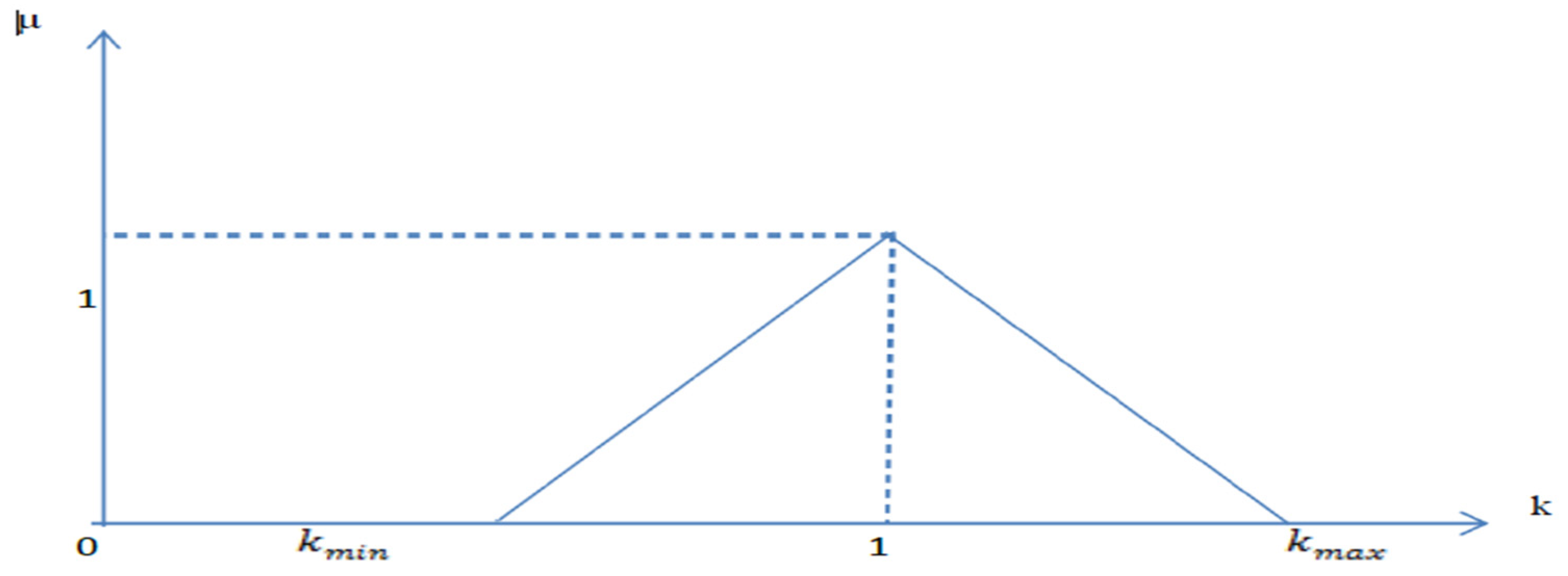
And the vagueness is a real triangular fuzzy number,

\tilde{K}

= {[0, ∞),

μ_{\tilde{K}}

};

μ_{\tilde{K}} (k) = \{\begin{matrix} \frac{k - k_{m i n}}{1 - k_{m i n}} k \in (k_{m i n}, 1) \\ \frac{k - k_{m a x}}{1 - k_{m a x}} k \in (1, k_{m a x}) \\ 0 otherwise \end{matrix}

0 < k_{m i n} \leq 1 \leq k_{m a x}

For a random variable T that follows a crisp Rayleigh distribution { Ray (

β

ξ

)}, the correspondent fuzzy random variable

\tilde{T}

with fuzzy Rayleigh probability distribution {

\tilde{R a y}

(

β

ξ

)}, with the followed features; for all 𝑡∈[0,∞), the fuzzy cumulative distribution function [1];

\tilde{F} (t) = 1 - e x p (- \frac{{{(t}_{i} - ξ)}^{2}}{2 \tilde{K} β^{2}})

(8)

Then for the 𝛼−𝑐𝑢𝑡 fuzzy distribution function where {

α

∈[0,1]}, we have

𝐹_{𝛼} (𝑡) = [𝐹_{1} 𝛼 (t), F_{2} 𝛼 (𝑡)] = {1 - 𝑒 xp - \frac{({t - ξ)}^{2}}{2 (1 - k m a x α + k m a x) β^{2}}, 1 - 𝑒 xp - \frac{{(t - ξ)}^{2}}{2 {(1 - k m i n α + k m i n) β}^{2}}}

(9)

Although the fuzzy reliability function is defined by ;

\tilde{R}

(𝑡) =

e x p (- \frac{{{(t}_{i} - ξ)}^{2}}{2 \tilde{K} β^{2}})

Then ∀𝛼∈ [0, 1) 𝑡ℎ𝑒 𝛼−𝑐𝑢𝑡𝑠 of fuzzy reliability function can be written every bit;

𝑅 𝛼 (𝑡) = [𝑅_{1} 𝛼 (𝑡), 𝑅_{2} 𝛼 (𝑡)] = [𝑒 xp - \frac{{(t - ξ)}^{2}}{2 (1 - k m i n α + k m i n {) β}^{2}}, 𝑒 xp - \frac{({t - ξ)}^{2}}{2 (1 - k m a x α + k m a x) β^{2}}]

(10)

4. Theoretical Part (Method of estimation)

In this section, we deal with six estimation methods for the parameters and the reliability function of two- parameters Rayleigh distribution

4.1. Maximum likelihood

This method is one of the most important methods of estimation that aims to make a possible function at the end of maximum. The method can be described as follows :

Write down the likelihood function L(

t_{i}, ξ, β

), and then find the value ̂ of that maximizes L(

t_{i}, ξ, β

; ). The log -likelihood function based on the random sampling of t₁ ,t₂ ,,,,,,t_n is specified by ;[14]:

L = \prod_{i = 1}^{n} f (t_{i}, ξ, β)

(11)

L = \frac{\prod_{i = 1}^{n} {(t}_{i} - ξ)}{β^{2}} e x p - \frac{{{(t}_{i} - ξ)}^{2}}{2 β^{2}}

(12)

Take the Natural for equation

(12)

logarithm for the previous likelihood function, so we get the following:

Ln L = - 2 n Ln β + \sum_{i = 1}^{n} L n {(t}_{i} - ξ) - \sum_{i = 1}^{n} \frac{{{(t}_{i} - ξ)}^{2}}{2 β^{2}}

(13)

But {\hat{ξ}}_{M L} = m i n {(t}_{i}) = t_{(1)} order statistics

(14)

Partial derivative of equation

(13)

for respect to unknown parameter β is:

\frac{\partial L n L}{\partial β} = \frac{- 2 n}{β} + \sum_{i = 1}^{n} \frac{{{(t}_{i} - ξ)}^{2}}{β^{3}}

(15)

Equate equation

(15)

to zero and we solve this equation:

\frac{- 2 n}{β} + \sum_{i = 1}^{n} \frac{{{(t}_{i} - ξ)}^{2}}{β^{3}} = 0 \frac{- 2 n {\hat{β}}^{2} + \sum_{i = 1}^{n} {{(t}_{i} - \hat{ξ})}^{2}}{{\hat{β}}^{3}} = 0 - 2 n {\hat{β}}^{2} + \sum_{i = 1}^{n} {{(t}_{i} - \hat{ξ})}^{2} = 0 2 n {\hat{β}}^{2} = \sum_{i = 1}^{n} {{(t}_{i} - \hat{ξ})}^{2} {\hat{β}}^{2} = \frac{\sum_{i = 1}^{n} {{(t}_{i} - \hat{ξ})}^{2}}{2 n} ∴ {\hat{β}}_{M L} = \sqrt{\frac{\sum_{i = 1}^{n} {{(t}_{i} - {\hat{ξ}}_{M L})}^{2}}{2 n}}

(16)

Then, according to different values of 𝛼−𝑐𝑢𝑡 estimate fuzzy, reliability function of the two-parameters Rayleigh distribution using Maximum likelihood method will be

{\hat{R}}_{M L} = e x p - \frac{{{(t}_{i} - {\hat{ξ}}_{M L})}^{2}}{2 \tilde{K} {\hat{β}}_{M L}^{2}}

(17)

4.2. Median-First Order Statistics (MD):

In this method, the second moment will be replaced by Me_t = t_me, wherever Me_t is the population median and t_me is the sample median [14]. The median of Rayleigh distribution with two parameters is as follows

0.5 = \int_{0}^{A} f (x) d t

(18)

\frac{1}{β^{2}} \int_{0}^{A} (t_{i} - ξ) e x p [- \frac{{{(t}_{i} - ξ)}^{2}}{2 β^{2}}] d t = \frac{1}{2}

A = ξ + β \sqrt{(2 l n 2)}

The cumulative distribution function of the random variable is

F_{t_{(1)}} t = P r [t_{(1)} < t] = 1 - P r [t_{(1)} > t)] = 1 - P r [t_{(1)} > t, t_{(2)} > t \dots \dots . . t_{(n)} > t] = 1 {- [p r (T > t)]}^{n} = 1 - {[R (t)]}^{n}

So, the cumulative distribution function of the random variable

t_{(1)}

f_{t_{(1)}} (t) = \frac{d F_{t_{(1)}}}{d t} = \frac{n (t - ξ)}{β^{2}} \exp [- \frac{{{(t}_{i} - ξ)}^{2}}{2 β^{2}}]; ξ < t < \infty, β > 0

For, the mathematical expectation of a random variable

t_{(1)}

this

The Median first order statistics method was proposed by Afify [2], to estimate the unknown parameters This method is based on the assumption that

E {[t}_{(1)}] = t_{(1)}

E {[t}_{(1)}] = \int_{ξ}^{\infty} \frac{t n (t - ξ)}{β^{2}} \exp [- \frac{{{(t}_{i} - ξ)}^{2}}{2 β^{2}}] d t = ξ + β \sqrt{\frac{π}{2 n}} {\begin{matrix} = t \end{matrix}}_{(1)} :

The first statistic represents the values of t .

(\hat{ξ}, \hat{β})

is unbiased estimator to

(ξ, β)

respectively then the equationrealized

\hat{ξ} = t_{(1)} - \hat{β} \sqrt{π / 2 n}

(19)

Thus, we have ξ + β \sqrt{(2 l n 2)} = t_{me}

(20)

ξ + β \sqrt{(2 l n 2)} = t_{m e} \to ξ = t_{m e} - β \sqrt{(2 l n 2)}

ξ + β \sqrt{π / 2 n} = t_{(1)} \to ξ = t_{(1)} - \sqrt{π / 2 n} β

t_{m e} - β \sqrt{(2 l n 2)} = t_{(1)} - β \sqrt{π / 2 n} \to t_{m e} - t_{(1)} = β \sqrt{(2 l n 2)} - β \sqrt{π / 2 n}

{\hat{β}}_{M d} = \frac{t_{m e} - t_{(1)}}{\sqrt{(2 l n 2)} - \sqrt{π / 2 n}}

(21)

From equation (20) and (21), we obtain

{\hat{ξ}}_{M d} = t_{m e} - {\hat{β}}_{M d} (\sqrt{(2 l n 2)})

(22)

Then according to different values of 𝛼− the estimate fuzzy reliability function of the two-parameters Rayleigh distribution using Median-First order Statistics Method(MD) will be

{\hat{R}}_{M d} = e x p - \frac{{{(t}_{i} - {\hat{ξ}}_{M d})}^{2}}{2 \tilde{K} {\hat{β}}_{M d}^{2}}

(23)

4.3. Quartile (QM)

Since the previous two methods use the smallest observance t ₍₁₎ X to estimate the location parameter

ξ

and the scale parameter

β

, therefore in the event that the minimum statistics is an outlier the estimation will be invalid. Our method is based on two approaches, the first one uses third and first quartile Q3and Q1, while the second one is based on third quartile and the median Q3and Med [16].

The first and third quartile of two-parameter Rayleigh distribution are:

Q 1 = ξ + β (\sqrt{l n (\frac{16}{9}))}

(24)

Q 3 = ξ + β (\sqrt{l n (16)})

(25)

Now solving (24) and (25) turn over the following estimation:

{\hat{β}}_{Q} = \frac{Q 3 - Q 1}{\sqrt{l n (16)} - \sqrt{l n (4 / 3)}}

(26)

{\hat{ξ}}_{Q} = Q 3 - {\hat{β}}_{Q} \sqrt{l n (16)}

(27)

T he first and third quartile of the sample are specifically ,Q1 , and Q 3

Now we consider the median and the third quartile case, the median can be written as

ξ + β \sqrt{(2 l n 2)} = m e d

(28)

From (24) and (27) we get

{\hat{β}}_{Q M} = \frac{Q 3 - m e d}{\sqrt{l n (16)} - \sqrt{l n (4)}}

(29)

{\hat{ξ}}_{Q M} = m e d - {\hat{β}}_{Q M} (\sqrt{l n (4)})

Then, according to different values of 𝛼−𝑐𝑢𝑡 estimation fuzzy reliability function of the two-parameter Rayleigh distribution using Median-First Order Statistics Method (Q, QM) will be

{\hat{R}}_{Q} = e x p - \frac{{{(t}_{i} - {\hat{ξ}}_{Q})}^{2}}{2 \tilde{K} {\hat{β}}_{Q}^{2}} a n d {\hat{R}}_{Q M} = e x p - \frac{{{(t}_{i} - {\hat{ξ}}_{Q M})}^{2}}{2 {\hat{\tilde{K} β}}_{Q M}^{2}}

(30)

4.4. L-Moments estimates (LM)

The method of Hosking [17] is used for L moments estimation. To write these estimations , let

X_{i : n}

denotes the ith order statistic for a sample of size n. Let

l_{1} = \frac{1}{n} \sum_{i = 1}^{n} X_{i : n} l_{2} = \frac{2}{n (n - 1)} \sum_{i = 1}^{n} {(i - 1) X}_{i : n} - l_{1}

Two first populations L-Moment are

λ_{1} = \sqrt{\frac{π}{2}} β + ξ, λ_{1} = 2 β^{2} + \sqrt{2 π} ξ β + ξ^{2}

. For more details seeGupta [11]

Now to get the LM of unknown parameters

ξ

and

β

we require the equal the sample L-Moment to with the populations L-Moment.

Hence the LM can be obtained from

l_{1} = \sqrt{\frac{π}{2}} β + ξ

(31)

l_{2} = 2 β^{2} + \sqrt{2 π} ξ β + ξ^{2}

(32)

First we obtain LME of

ξ, s a y {\hat{ξ}}_{L M}

as solution of the following non-linear equation

\frac{l_{2}}{l_{1}} = \frac{2 β^{2} + \sqrt{2 π} ξ β + ξ^{2}}{\sqrt{\frac{π}{2}} β + ξ}

(33)

Once

{\hat{ξ}}_{L M}

is obtained the LM of

β

say

{\hat{β}}_{L M}

can be obtain from (31) as

{\hat{β}}_{L M} = \frac{\sqrt{\frac{π}{2}} β + ξ}{l_{1}}

(34)

We can obtain a solution numerical through the equation ( 33 )and (34) non-linear equation by using F solve in Matlab2018 b.

Then, according to different values of 𝛼−𝑐𝑢𝑡 estimate fuzzy reliability function of the two-parameters Rayleigh distribution using L-Moments(LM) is

{\hat{R}}_{L M} = e x p - \frac{{{(t}_{i} - {\hat{ξ}}_{L M})}^{2}}{2 \tilde{K} {\hat{β}}_{L M}^{2}}

(35)

4.5. Mixed Thompson-Type Shrinkage Estimator(MX)

The shrinkage estimation method is the Bayesian approach depending on prior information regarding the value of the specific parameter

θ

from past experiences or previous works .However, in certain situations prior information is usable only from of an initial guess value (natural origin)

θ_{°}

θ

[18]. In such situation, it is natural to start with an estimator

\hat{θ}

(e.g., MLE) of

θ

and modify it by moving it closer to

θ_{°}

.Thompson has suggested the problem of shrink a classical estimator

\hat{θ}

of the parameter

θ

toward prior information (a natural origin)

θ_{°}

by shrinkage estimator

ψ (\hat{θ}) \hat{θ} + (1 - ψ (\hat{θ})) θ_{°}

, 0

\leq ψ (\hat{θ}) \leq 1

, which is more efficient than

\hat{θ}

θ_{°}

is close to

θ

and less efficient than

\hat{θ}

otherwise.

According to Thompson [24]

θ_{°}

is a natural origin andmay arise from any one of number of reasons—e.g., we are estimating

θ

and (a) we believe

θ_{°}

is close to the true value of

θ

, or (b) our fear that

θ_{°}

may be near the true value of

θ

, that means something bad happens if

θ_{°} = θ

, and we donot know about it (that is, something bad happens if

θ_{° \approx} θ

and we do not use

θ_{°})

And,

ψ (\hat{θ})

is so called shrinkage weight factor; 0

\leq ψ (\hat{θ}) \leq 1

which represents the belief of

\hat{θ}

,and (1-

ψ (\hat{θ})

) it represents the belief of

θ_{°}

.Thompson notes that the shrinkage weighting element may be a function of

\hat{θ}

or may be constant and the chosen of the shrinkage weight factor is ad hoc basis.

Also, the shrinkage weight function

ψ (\hat{θ})

can be found by minimizing the mean square error of

\tilde{θ}

M S E ({\tilde{θ}}_{T H}) = E {({\tilde{θ}}_{T H} - θ)}^{2}

(36)

= E {(ψ (\hat{θ}) {\hat{θ}}_{M L} + (1 - ψ (\hat{θ})) θ_{°} - θ)}^{2}

The partial derivative for equation

(36)

w .r. t. to

ψ (\hat{θ})

\frac{\partial M S E (\tilde{θ})}{\partial ψ (\hat{θ})} = 2 ψ (\hat{θ}) E {({\hat{θ}}_{M L} - θ_{°})}^{2} - 2 (1 - ψ (\hat{θ})) {({\hat{θ}}_{M L} - θ_{°})}^{2}

(37)

Equating equation

(38)

to zero and we solve this equation:

\frac{\partial M S E (\tilde{θ})}{\partial ψ (\hat{θ})} = 0

2 ψ (\hat{θ}) M S E ({\hat{θ}}_{M L}) - 2 (1 - ψ (\hat{θ})) {({\hat{θ}}_{M L} - θ_{°})}^{2} = 0

ψ (\hat{θ}) = \frac{{({\hat{θ}}_{M L} - θ_{°})}^{2}}{[M S E ({\hat{θ}}_{M L}) + {({\hat{θ}}_{M L} - θ_{°})}^{2}]}

(38)

Suppose that

θ_{°} = {\hat{θ}}_{L M}

Therefore, the shrinkage estimators of

ξ

and

β

are respectively becomes as below:

{\hat{ξ}}_{M X} = {\hat{ξ}}_{L M}_{°} + \frac{{({\hat{ξ}}_{M L} - {\hat{ξ}}_{L M})}^{3}}{[M S E ({\hat{ξ}}_{M L}) + {({\hat{ξ}}_{M L} - {\hat{ξ}}_{L M})}^{2}]}

(39)

{\hat{β}}_{M X} = {\hat{β}}_{L M}_{°} + \frac{{({\hat{β}}_{M L} - {\hat{β}}_{L M})}^{3}}{[M S E ({\hat{β}}_{M L}) + {({\hat{β}}_{M L} - {\hat{β}}_{L M})}^{2}]}

(40)

Then according to different values of 𝛼−𝑐𝑢𝑡 estimate fuzzy reliability function of the two-parameters Rayleigh distribution using Mixed Thompson-Type Shrinkage (MX)are

{\hat{R}}_{M X} = e x p - \frac{{{(t}_{i} - {\hat{ξ}}_{M X})}^{2}}{2 \tilde{K} {\hat{β}}_{M X}^{2}}

(41)

5. Practical part

5.1. Simulation Study

We carried out a Monte Carlo simulation in order to compare the performance of all the estimators that proposed in the preceding part. The programs are written in Matlab (2017b). The results are based on 1000 simulations runs. Random samples of different sizes by observing that if U is uniform (0, 1), then

t = ξ + β {[- 2 l o g (1 - U)]}^{\frac{1}{2}}

is Rayleigh of (

ξ

, β) are generated. The sample sizes are considered were n=25, 50, 75, 100.

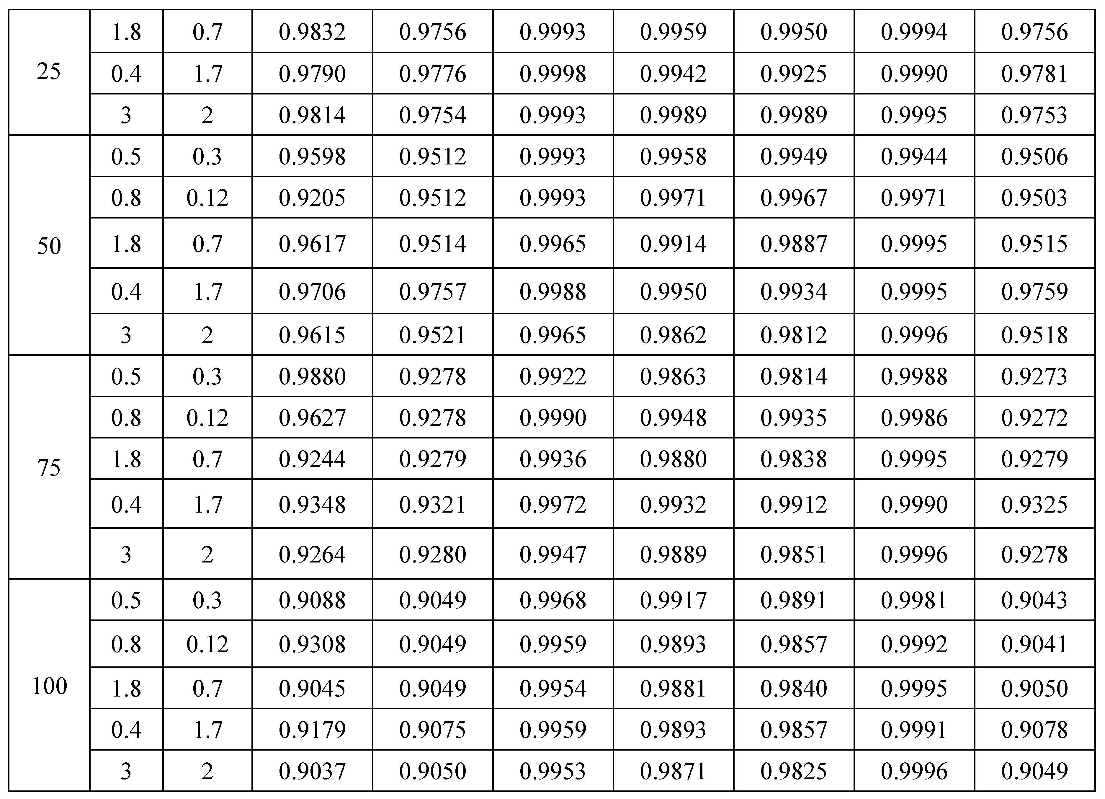
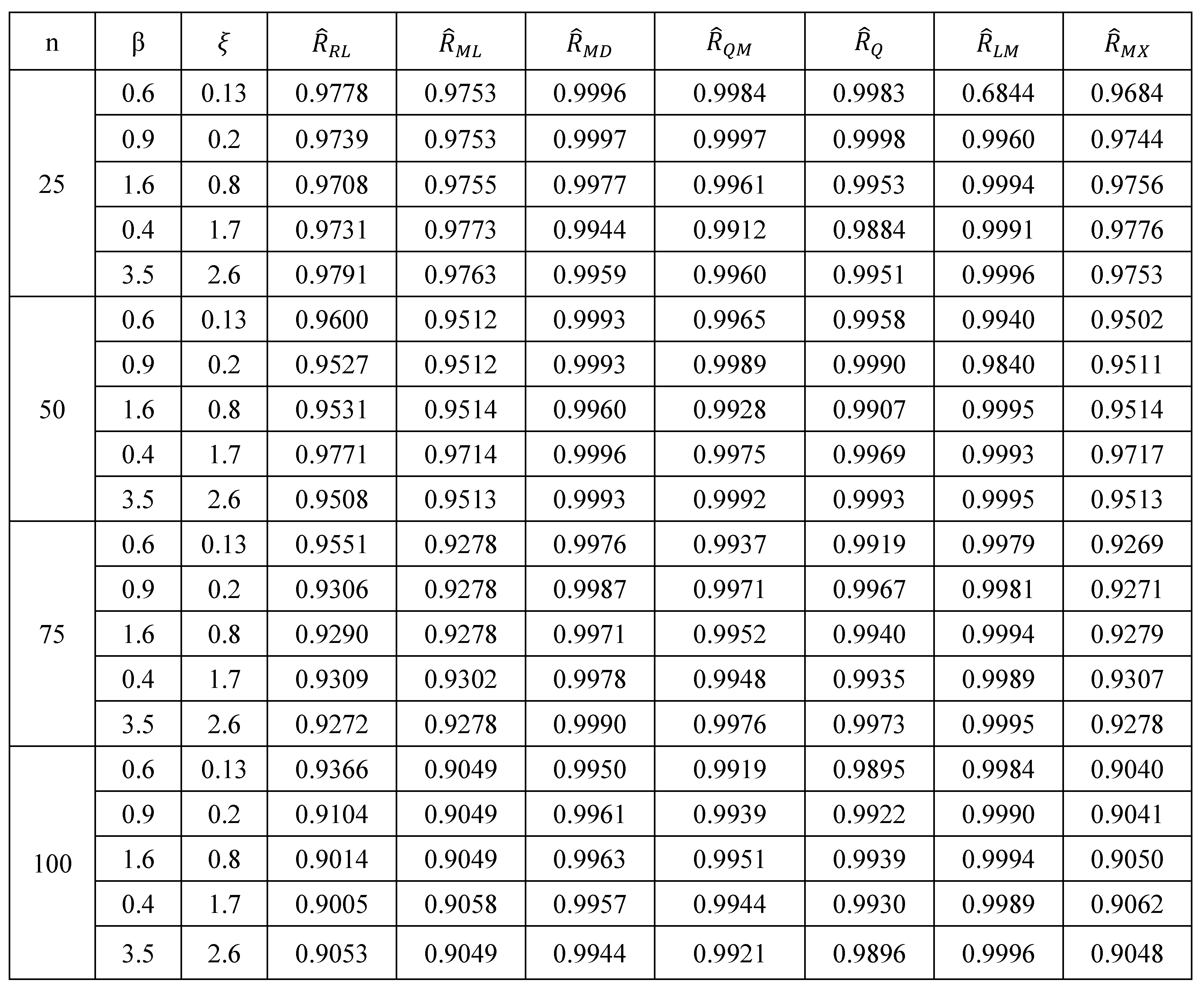
We used 1000 replications to estimate by using the ML, MD,QM Q ,LM and MX methods. The process of simulation strategy is explained the numerical results in the Table 1, Table 2, Table 3, Table 4 and Table 5. And comparison are made among all proposes estimators fuzzy reliability. After that we make the randomized fuzzy values

t_{i}

of the CDF function indicated by the size of the given samples and the default values of initial parameters according to the formula

\tilde{R} (t_{i})

, the values of

t_{i}

and the initial parameters were computed according to the function of the

μ_{\tilde{t_{i}}}

(t) for each fuzzy unit

t_{i}

.Then, extract for each

\tilde{R} (t_{i})

and find expectation of

\tilde{R} (t_{i})

as follows:

\tilde{R} (t) = \hat{E} (\frac{\tilde{R} (t_{i})}{\tilde{x_{i}}}) = \frac{1}{Q} \sum_{h = 1}^{Q} R^{h} (t) w h e r e Q = 1000 a n d h = 1 \dots \dots \dots \dots . Q

F u z z y r a n d o m v a r i a b l e (\tilde{T}) a r e f u z z y n u m b e r e d, \tilde{t} = k t

Statistical measures Mean Squared Error is

m s e (\tilde{R}) = \frac{1}{K} \sum_{h = 1}^{q} {(\tilde{R} - R)}^{2}

5.2. Numerical Analysis

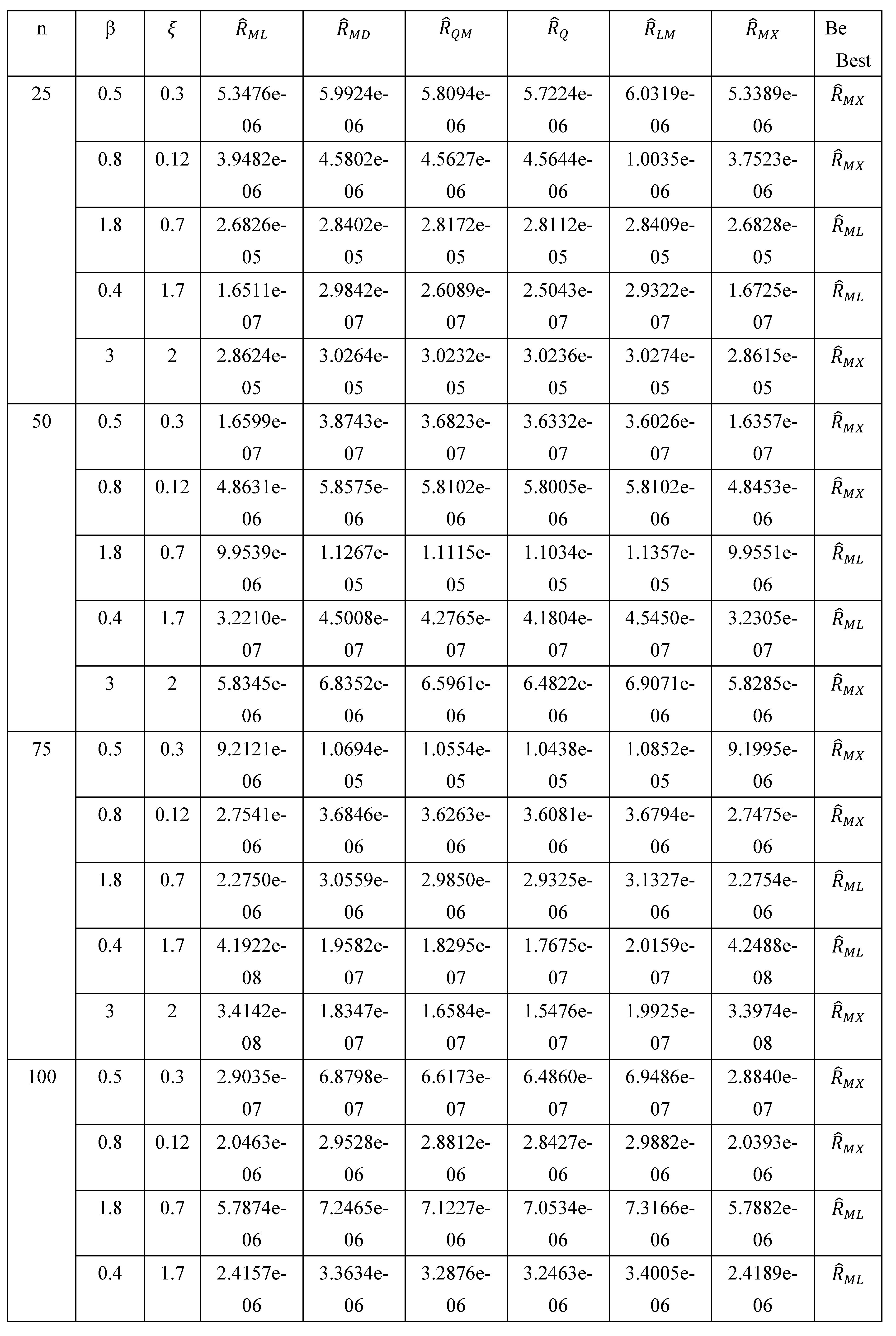
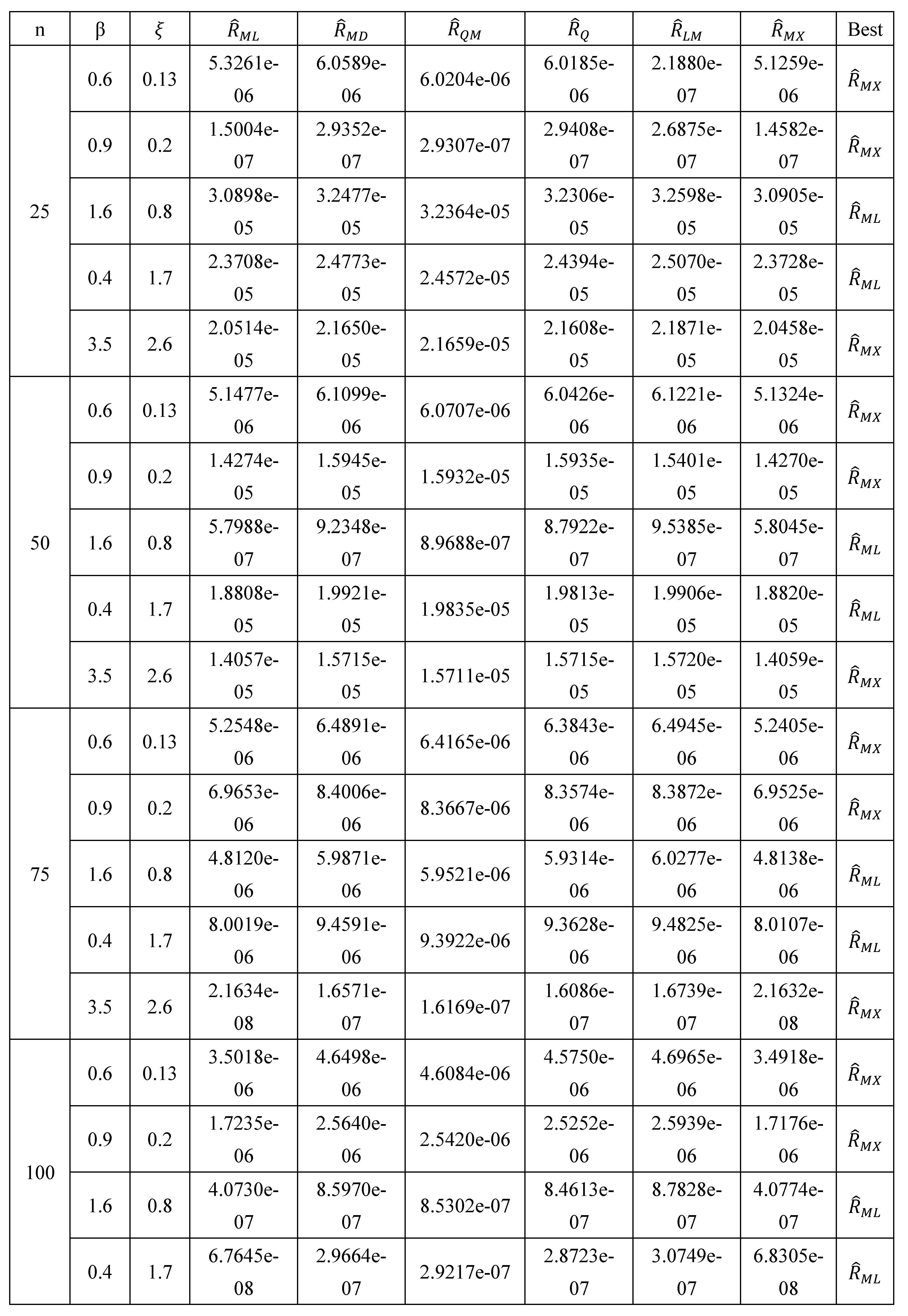
If we use K=0.4 n=25,50,75,100 ,

ξ

=(0.3, 0.12 ,2) and , β=(0.5 ,0.8 ,3) the estimator

{\hat{R}}_{M X}

preforms good and will best than the other estimators in the sense of MSE, and it follows by

{\hat{R}}_{M L}

{\hat{R}}_{M D}

, {\hat{R}}_{Q}

{\hat{R}}_{Q M}

a n d {\hat{R}}_{L M}

for all

ξ

and β.

If we use K=0.4, n=25,50,75,100, $ξ$ =(0.7, 1.7) and , β=(1.8 ,0.4) we can see in the Table (4) , the MSE of estimator ${\hat{R}}_{M L}$ is less than of the MSE of the other estimators , thus it will be the best in the sense of MSE and it follows by the estimators by ${\hat{R}}_{M D}$ , ${\hat{R}}_{Q}$ $, {\hat{R}}_{Q M,}$ $, {\hat{R}}_{L M}$ and ${\hat{R}}_{M X}$ .
If we use K=0.7 ,n=25,50,75,100 , $ξ$ =(0.13, 0. 2 ,2.6) and , β=(0.6 ,0.9 ,3.5) the estimator ${\hat{R}}_{M X}$ preforms good and will best than the other estimators in the sense of MSE, it follows by ${\hat{R}}_{M L}$ , ${\hat{R}}_{M D}$ $, {\hat{R}}_{Q}$ ${\hat{R}}_{Q M}$ $a n d {\hat{R}}_{L M}$ for all $ξ$ and β.
If we use K=0.7 n=25,50,75,100, $ξ$ =(0.8, 1.7) and , β=(1.6 ,0.4) we can see in the Table (5) , the MSE of estimator ${\hat{R}}_{M L}$ is less than of the MSE of the other estimators , thus it will be the best in the sense of MSE and it follows by the estimators by ${\hat{R}}_{M D}$ , ${\hat{R}}_{Q}$ $, {\hat{R}}_{Q M,}$ $, {\hat{R}}_{L M}$ and ${\hat{R}}_{M X}$ .

6. Conclusions

From all Tables, one can be noticed that, the Maximum likelihood Method, and Mixed Thompson Method, perform better than the other methods in the sense of MSE, and we recommend to use this type of estimation. Also , as accomplished, the fuzzy estimator of (R) is better than the conventional estimator subsequently it contains the entire variable under consideration.

References

K. S.. Bohra , S. B. Singh.” Evaluating fuzzy system reliability using intuitionistic fuzzy Rayleigh lifetime distribution”, Mathematics In Engineering, Science and AerospaCE,6(2) 245- 254 ,2015.
L. A. Zadeh.”Fuzzy sets. Information and Control”. 8, 338 -353, 1965.
K. T. Atanassov. “Intuitionistic fuzzy sets”, VII ITKR s Session, Sofia deposed in Central Sci.-Technical Library of Bulg, Acad. of Sci. 1697/84, 1983.
Cai, K. Y., Wen, C. Y., Zhang, M. L.Fuzzy variables as a basis for a theory of fuzzy reliability in the possibility context. Fuzzy Sets and Systems, 42, 145–172 ,1991.
Cai, K. Y., Wen, C. Y., Zhang, M. L. “Fuzzy states as a basis for a theory of fuzzy Reliability”. Micro electron. Reliab, 33, 2253–2263, (1993). [CrossRef]
Cai, K. Y., Wen, C. Y., Zhang, M. L.” Coherent systems in profust reliability theory, In: Onisawa T., Kacprzyk J. (eds) Reliability and Safety Analyses under Fuzziness. Studies in Fuzziness”, vol 4. Physica, Heidelberg. [CrossRef]
Karpisek, Z., Stepanek, P., Jurak, P. “Weibull fuzzy probability distribution for reliability of Concrete structures”. Engineering mechanics, 17(5/6), 363–372, 2010.
Baloui J., E. “An evaluation of the systems reliability using fuzzy lifetime, 2011. Distribution”. Journal of Applied Mathematics, Islamic Azad University of Lahijan, 7(28), 73-80.
Baloui. J., E. “Reliability estimation under the fuzzy environments”. The Journal of Mathematics and Computer Science, 5 (1), 28-39, 2012.
Rezvani, S. “A new method for ranking in perimeters of two generalized trapezoidal fuzzy numbers”. International Journal of Applied Operational Research, 2(3), 85-92.,2012.
Nathier. A. I, Hussein.A..M, “ Parameters and Reliability Estimation for the Fuzzy Exponential” Distribution, American Journal of Mathematics and Statistics, 7(4): 143-151, 2017.
Hsien, C.. W.”Fuzzy reliability estimation using Bayesian approach”, Computers &Industrial Engineering 46(3), 467–493, 2004.
R. Seising “Proposals for Future Developments in Fuzzy Set Technology, Fuzzy Systems”, IEEE International Conference, 2006.
TAHA.A “On Reliability Estimation for the Rayleigh Distribution Based on Monte Carlo Simulation” International Journal of Science and Research (IJSR) ISSN (Online): 2319-7064, 2015.
Mouloud.G, Ahmed. H and Ben Rahmoune. M,” Reliability modeling using Rayleigh distribution: Industrial pump application”. Proceedings of the 19th European Conference on Mathematics for Industry ECMI2016, 13-17th June 2016, Santiago de Compostela, Spain.
Entisar.A. and Nadia. B. “ Quartile Method Estimation of Two- Parameter Exponential Distribution Data with Outliers” International Journal of statistics and probability,5 ( 5),2016.
J.R.M. Hosking. “L-moment: Analysis and estimation of distributions using linear combinations of order statistics”, J. R. Stat. Soc. Ser. B 52 105–124 ,1990. [CrossRef]
Thompson, J.R. ”Some Shrinkage Techniques for Estimating the Mean”. J. Amer. Statist. Assoc., 63, 113-122.,1968.
L. A. Zadeh.”Fuzzy sets. Information and Control”. 8, 338 -353, 1965.
Afify, E. E.”Linear and Nonlinear regression of exponential distribution”. Inter. Statist., online Statistics Journal Cohen, A. C., &Helm, F. R. Estimation in Exponentia Distribution. Technometrics,15, 415-418 ,. 2004.
Gupta, R. D. and Kundu, D. “Generalized exponential distributions: different method of estimation, Journal of Statistical Computation and Simulation”. 69, 315 – 338, 2001b. [CrossRef]
A.N..Salman “Pre-test single and double stage shrunken estimators for the mean of normal distribution with known variance”. Baghdad Journal for Science, 7(4), (1432– 1442),2010.
Castillo, Oscar, Melin, Patricia. “Type-2 Fuzzy Logic: Theory and Applications, Studies in Fuzziness and Soft Computing”. Springer, 2008.
Dalalah. D, Magableh. S “A remote fuzzy multi-criteria diagnosis of sore throat”, Telemed J E Health,(2008).

Table 1. The value β,

ξ

and K

Table 1. The value β,

ξ

and K

Table 2. Estimate fuzzy reliability of Rayleigh distribution is Based on simulations K=0.4.

Table 3. Estimate fuzzy reliability of Rayleigh distribution is based on simulations K=0.7.

Table 4. Mean squared error (MSE) of fuzzy reliability estimates is based on simulations K=0.4.

Table 5. Mean squared error (MSE) of fuzzy reliability estimates is based on simulations K=0.7.

Disclaimer/Publisher’s Note: The statements, opinions and data contained in all publications are solely those of the individual author(s) and contributor(s) and not of MDPI and/or the editor(s). MDPI and/or the editor(s) disclaim responsibility for any injury to people or property resulting from any ideas, methods, instructions or products referred to in the content.

© 2023 by the authors. Licensee MDPI, Basel, Switzerland. This article is an open access article distributed under the terms and conditions of the Creative Commons Attribution (CC BY) license (http://creativecommons.org/licenses/by/4.0/).

Copyright: This open access article is published under a Creative Commons CC BY 4.0 license, which permit the free download, distribution, and reuse, provided that the author and preprint are cited in any reuse.

Alerts

MDPI Initiatives

Important Links

Choose an area of interest and we will send you notifications of new preprints at your preferred frequency.

Disclaimer

Comparison Different Estimation Method for Reliability Function of Based On Fuzzy Lifetime Data

Abstract

Keywords:

Subject:

1. Introduction

2. Essential Definitions

3. Rayleigh Distribution Function

4. Theoretical Part (Method of estimation)

4.1. Maximum likelihood

4.2. Median-First Order Statistics (MD):

4.3. Quartile (QM)

4.4. L-Moments estimates (LM)

4.5. Mixed Thompson-Type Shrinkage Estimator(MX)

5. Practical part

5.1. Simulation Study

5.2. Numerical Analysis

6. Conclusions

References

MDPI Initiatives

Important Links

Subscribe