
Submitted:
16 October 2023
Posted:
17 October 2023
You are already at the latest version
Abstract
This paper is primarily focused on the robust control of an inverted pendulum system based
on the policy iteration in reinforcement learning. First, a mathematical model of the single inverted
pendulum system is established through a force analysis of the pendulum and trolley. Second,
based on the theory of robust optimal control, the robust control of the uncertain linear inverted
pendulum system is transformed into an optimal control problem with an appropriate performance
index. Moreover, for the uncertain linear and nonlinear systems, two reinforcement-learning control
algorithms are proposed using the policy iteration method. Finally, two numerical examples are
provided to validate the reinforcement learning algorithms for the robust control of the inverted
pendulum systems.
Keywords:
robust control
; optimal control
; inverted pendulum system
; reinforcement learning
1. Introduction
In the last decade, there has been an increasing interest in the robust control of the inverted pendulum system (IPS) owing to its high potential in testing a variety of advanced control algorithms. Robust control is widely used in power electronic [1], flight control [2], motion control [3], network control [4], and IPSs [5], in addition to other fields. The research on the robust control of an IPS has provided advantageous results in recent years. An inverted pendulum is an experimental device having insufficient drive, absolute instability, and uncertainty. It has become an excellent benchmark in the field of automatic control over the last few decades as it provides better explanations for model-based nonlinear control techniques and is a typical experimental platform for verifying classical and modern control theories [6].
Although the earliest research on the IPS can be traced back to 1908 [7], there was almost no literature on this subject between 1908 and 1960. Until 1960, a number of tall, slender structures survived the Chilean earthquake, while structures that appeared more stable were severely damaged. Therefore, some scholars conducted more in-depth research to obtain a suitable explanation [8]. The pendulum structure under the effect of earthquakes is modeled as a base and rigid block system, and block overturning is studied by applying a horizontal acceleration, sinusoidal pulses, and seismic-type excitations to the system. It was observed that there is an unexpected scaling effect that makes the large block more stable than the small block among two geometrically similar blocks. Furthermore, tall blocks exhibit greater stability during earthquakes when exposed to horizontal forces. Since then, with the development of modern control theory, various control methods have been applied to different types of IPSs, such as the proportional-integral–derivative control [9,10], cloud model control [11,12], fuzzy control [13,14,15,16], sliding mode control [17,18], and neural network control methods [19,20,21]. These methods provide different ideas for the control of IPSs.
As is known, the IPS is an uncertain system, and the uncertainty of its model is naturally within the scope of consideration. The aim of the robust control of an IPS is to find a controller capable of addressing system uncertainties. When the system is disturbed by uncertainty, robust control laws can stabilize the system. Because it is difficult to directly solve the robust control problem, Lin et al. transformed the robust control problem into an optimal control problem [22,23,24]. However, the pioneering methods for solving optimal control problems mainly include the dynamic programming [25] and maximum principle [26] methods. In the dynamic programming method, solving the Hamilton–Jacobi–Belman (HJB) equation yields the optimal control of the system. However, the HJB equation is a nonlinear partial differential equation, and obtaining its solution has proven to be more difficult than solving the optimal control problem. As for the optimal control problem of a linear system with a quadratic performance index, irrespective of whether it is a continuous system or a discrete system, it finally comes down to solving an algebraic Riccati equation (ARE). However, when the dimension of the state vector or control input vector in the dynamic system is large, the so-called "curse of dimensionality" appears when the dynamic programming method is used to solve the optimal control problem [27]. To overcome this weakness, some scholars have proposed the use of the reinforcement learning (RL) policy to solve the optimal control problem [28,29].
When RL was initially used for system control, it was primarily focused on discrete-time systems or discretized continuous-time systems in research on problems such as the billiard game problem [30], scheduling problem [31,32,33], and robot navigation problem [34]. Furthermore, the application of RL algorithms to continuous-time and continuous-state systems was initially extended by Doya et al. [35]. They used the known system model to learn the optimal control policy. In the context of control engineering, the RL and adaptive dynamic programming link traditional optimal control methods with adaptive control methods [36,37,38]. Vrabie et al. [39] used the RL algorithm to solve the optimal control problem of the continuous time system. In the case of the linear system, the system data is collected, and the solution of the HJB equation is obtained via online policy iteration (PI) using the least squares method. Xu et al. [40,41] proposed an RL algorithm based on linear and nonlinear continuous-time systems to solve the robust tracking problems through online PI. The algorithm takes into consideration the uncertainty in the system’s state and input matrices and improves the method for solving robust tracking.
The use of the RL method to iteratively solve the optimal control problem has attracted extensive attention from scholars and resulted in relatively good results. The IPS demonstrates a positive impact in the validation of advanced control algorithms. Although there is a significant amount of literature on the IPS [9,11,15], to the best of our knowledge, there are almost no research results comprising the use of the RL for solving the control of IPS. In this study, an attempt is made to solve the robust control problem of an uncertain continuous-time IPS using the RL algorithm. The dynamic equations of the nominal system need not be known when using the RL control algorithm, and this study lays a theoretical foundation for the wide application of the RL control algorithm in engineering systems. The main contributions of this study are as follows.
1) The state space model of the IPS is established and a robust optimal control design method for uncertain systems is proposed. By constructing appropriate performance indicators, the optimal control method is used for the first time to design a robust control law for an uncertain IPS, which is an original approach.
2) A PI algorithm in the RL has been designed for realizing the robust optimal control of an IPS. The use of RL algorithms to solve the robust control problem of the IPS does not require that the nominal system matrix be known, and it can also overcome the challenges resulting from the "curse of dimensionality.’’ The first application of the RL for solving the control problem of an IPS has significance for its potential application in practical engineering.
The organization of this paper is as follows. In Section 2, the state-space equation of the IPS and a linearization model are established. The robust control and RL algorithm for linearized the IPS are presented in Section 3 and 4. In Section 5, we establish the nonlinear state-space model of the IPS and propose the corresponding RL algorithm. The RL algorithm is then verified via a simulation in Section 6. Finally, we summarize the work of this paper and potential future research directions.
2. Preliminaries
In this section, we established a physical model of a first-order linear IPS according to Newton’s second law. By selecting appropriate state variables, the state space model with uncertainty is derived.
2.1. Modeling of Inverted Pendulum System
The inverted pendulum experimental device comprises a pendulum and a trolley. Its structure is presented in Figure 1. Moreover, its simplified physical model is presented in Figure 2, which mainly includes the pendulum and trolley. In Figure 2, owing to the interaction between the trolley and pendulum, the trolley is subjected to a force from the pendulum, which acts in the lower left direction. Furthermore, the pendulum is subjected to a force from the trolley, which acts in the upper right direction. In addition, the pendulum and trolley are also subjected to other forces, as shown in Figure 3 and 4, respectively. The trolley is driven by a motor to perform horizontal movements on the guide rail. In Figure 3, the trolley is subjected to the force from the motor and gravity. represents the resistance between the trolley and guide rail. Furthermore, and are the two components of force . In Figure 4, the pendulum is subjected to gravity , and and are the two components of force .
To facilitate subsequent calculations, we define the parameter of the first-order IPS, as shown in Table 1. The time parameter symbol is omitted, which indicates that x represents . According to Newton’s second Law, in the horizontal direction, the trolley satisfies the following equation

Table 1.
IPS parameter symbols.
| Parameter | Unit | Significance |
|---|---|---|
| Mass of the trolley | ||
| Mass of the pendulum | ||
| L | m | Half the length of the pendulum |
| z | Friction coefficient between the trolley and guide rail | |
| x | m | Displacement of the trolley |
| Angle from the upright position | ||
| I | Moment of inertia of pendulum |
We assume that the resistance is proportional to the speed of the trolley. Therefore, , z is the proportional coefficient. Moreover, in the horizontal direction, the pendulum satisfies the following equation
Considering that , and on substituting (2) into (1), we obtain
Next, we analyze the resultant force in the vertical direction of the pendulum, and the following equation can be obtained.
The component force of in the direction perpendicular to the pendulum is
Based on the torque balance, we can obtain the following equation
where I is the moment of inertia of the pendulum. On substituting equations (4) and (5) into Equation (6),
Thus far, equations (3) and (7) constitute the dynamic model of the IPS. Moreover, it can be assumed that the rotation angle of the pendulum is very small, that is, . Therefore, it can be approximated that
Therefore, it follows from equations (3) and (7),
2.2. State Space Model with Uncertainty
In Section 2.1, we established the dynamic model of the IPS as shown in Equation (8). Next, we will derive the state space model of the IPS.
As the rotation angle of the pendulum is very small, it can be approximated that , . It follows from (8) that
The state variables of the system can be defined as
Therefore, the following state space equation can be derived.
where u represents the force from the motor. Using , Equation (10) can be written as
where
However, the accurate model of the IPS is difficult to obtain, and all its parameters have uncertainties. In this paper, the friction coefficient z between the trolley and guide rail is selected as an uncertain parameter. The numerical values of the other parameters in Table 1 are known, where . Therefore, the state space model of the uncertain IPS can be abbreviated as
where
Here we choose as the nominal value and denote the nominal matrix of the system as . Therefore, the nominal system corresponding to the uncertain system (11) is
where
3. Robust Control of Uncertain Linear System
This section mainly presents with robust optimal control methods for the uncertain IPS modeled in the previous section by selecting the appropriate performance index function and solving an ARE to construct the robust control law. When the uncertain parameters of the system change within a certain range, this robust control law can cause the system to become asymptotically stable.
The following lemmas are proposed to prove the main results of this paper.
Lemma 1.
The nominal system (12) corresponding to system (11) is stabilizeable.
Proof.
For the four-dimensional continuous time-invariant system presented in system , the controllability matrix is constructed as
Therefore, we have
Therefore, system (12) is completely controllable, which means that the system can be stabilized. This concludes the proof. □
Lemma 2.
There is an matrix , such that the system matrices and satisfy the following matched condition.
Proof.
where
This concludes the proof. □
Lemma 3.
For any , there exists a positive semidefinite matrix F, such that satisfies
where .
Proof.
According to lemma 2, we can obtain
This concludes the proof. □
For nominal system (12), we construct the following ARE.
where . According to the above three lemmas and ARE (18), we propose the following theorem.
Theorem 1.
Let us suppose that S is a symmetric positive definite solution to ARE (18). Then, for all uncertainties , the feedback control , can make the system (11) asymptotically stable.
(Proof of Theorem 1).
We define the following Lyapunov function.
We set and take the time derivative of the Lyapunov function (19) along the system (11). We can then obtain
According to Lemma 2, we can obtain
On substituting ARE (18) into the above equation, we obtain
because ,
As
we can obtain
Therefore,
According to the Lyapunov stability theorem, the uncertain system (11) is asymptotically stable. Theorem 1 has thus been proved. □
4. RL Algorithm for Robust Optimal Control
In this section, we propose an RL algorithm for solving the robust control problem of an IPS through online PI. According to ARE (18), the following optimal control problem is constructed. For the nominal system,
we find a control u, such that the following performance index reaches a minimum.
where . For any initial time t, the optimal cost can be written as
From Lyapunov function (19), we obtain
where S is the solution to ARE (18). We propose the following RL algorithm for solving a robust controller.
Algorithm 1.RL algorithm for robust control of uncertain linear IPS
- (1)
- is computed.
- (2)
- An initial stabilization control gainis selected.
- (3)
- Policy evaluation:is solved using the equation.
- (4)
- Policy improvement:.
- (5)
- We set, and steps 3 and 4 are repeated until, whereis a small constant.
In Algorithm 1, by providing an initial stabilizing control law, repeated iterations are performed between steps 3 and 4 until convergence. We can then obtain the robust control gain K of system (11).
Remark 1.
Step 3 in Algorithm 1 is the policy evaluation, and step 4 is the policy improvement. Equivalently, the solving of the equation in step 3 is actually solving a least squares problem. In the integral interval, if sufficient data are obtained in the system, the least square method can be used to solve . Although it is also possible to directly solve the ARE (18) to obtain , the state matrix of the system (12) is required to be known. The implementation of Algorithm 1 does not necessitate that the state matrix of the system be known.
Next, we prove the convergence of Algorithm 1. However, it is necessary to prove the following Lemma first.
Lemma 4.
On assuming that the matrix is stable, solving the matrix from step 3 of Algorithm 1 becomes equivalent to solving the following equation.
Proof. We rewrite the equation of step 3 in Algorithm 1 as follows
According to the definition of the derivative, it can be observed that the first term of Equation (23) is the derivative of with respect to time t. We thus obtain
Further re-arranging Equation (24) yields
which means that (22) is established. Next, we reverse the process.
Along the stable system , the time derivative of the Lyapunov function is calculated. We can then obtain
On integrating both sides of the above equation in the interval , we obtain
This concludes the proof.
According to the existing conclusions [42], iterative relations (22) and step 3 of Algorithm 1 converge to the solution of ARE (18).
5. Robust Control of Nonlinear IPS
In this section, we establish a nonlinear state-space model of the IPS and construct an appropriate auxiliary system and a performance index. The problem of the robust control of the IPS is then transformed into the optimal control problem of the auxiliary system. We finally propose the corresponding RL algorithm.
5.1. Nonlinear State-Space Representation of IPS
Based on the uncertain linear inverted pendulum model (11) established in Section 2.1, we consider the following uncertain nonlinear system.
where represents the nonlinear perturbation of the system and can be used to represent various nonlinearity factors in the system. Based on the modeling process in Section 2 and literature [23], it is assumed that
where the parameters I, , L, and W are the same as those in (10). On rewriting system (26), we obtain
where
On substituting the parameter values into system (27), we can obtain
5.2. Robust Control of Nonlinear IPS
To obtain the robust control law for an uncertain nonlinear IPS, we propose the following two lemmas.
Lemma 5.
There exists an uncertain function such that can be decomposed into the following form.
Proof.
where . Proof completed. □
Lemma 6.
There exists an upper bound function such that satisfies
Proof.
This concludes the proof. □
We constructing the optimal control problems for a nominal system.
We determine a controller u such that to minimize the following performance index.
According to the performance index function (30), the cost function corresponding to the admissible control policy is
Taking the time derivative on both sides of function (31) yields the following Bellman equation.
where is the gradient of the cost function with respect to x.
We define the following Hamiltonian function.
On assuming that the minimum exists and is unique, the optimal control function for the given problem is then obtained as
On substituting Equation (34) into Equation (32), the HJB equation that satisfies the optimal function can be obtained as
with the initial condition .
On solving the optimal function from Equation (35), the solution of the optimal control problem can be obtained. The solution of the robust control problem can then be obtained. The following theorem shows that the optimal control is a robust controller for a nonlinear IPS.
Theorem 2.
On considering the nominal system (29) with the performance index (30) and assuming that solution of the HJB Equation (35) exists, the optimal control law (34) can then globally stabilize the IPS (27).
(Proof of Theorem 2).
We select as the Lyapunov function. On considering the performance index function (30), is obviously positive definite, and . Taking the time derivative of along system (27) yields
According to Lemma 5, it follows that
According to HJB Equation (35), we can obtain
From Equation (38), we can obtain
where . According to the Lyapunov stability criterion, the optimal control (34) can make the uncertain nonlinear IPS (27) asymptotically stable for all the allowable uncertainties. Therefore, for a constant , there is a neighborhood of the origin, such that, if the state enters the neighborhood , then when . However, cannot remain outside the domain forever; else, for all , which implies that
Let , then
5.3. RL Algorithm for Nonlinear IPS
For a nonlinear IPS, we consider the optimal control problems (29) and (30). For any admissible control, the cost function corresponding to the optimal control problem can be expressed as
where is an arbitrarily selected constant. We can then obtain the integral reinforcement relation satisfied by the cost function
Based on the integral-based reinforcement relations (40) and the optimal control (34), the RL algorithm for the robust control of the nonlinear IPS is given below.
Algorithm 2.RL algorithm for robust control of uncertain nonlinear IPS
- (1)
- A non-negative functionis selected.
- (2)
- An initial stabilization control lawis selected.
- (3)
- Policy evaluation: thefromis solved.
- (4)
- Policy improvement:.
- (5)
- is set and steps 3 and 4 are repeated until, whereis a small constant.
In Algorithm 2, by providing an initial stabilizing control law, the algorithm iterates repeatedly between steps 3 and 4 until convergence. We can then obtain the robust control gain u of system (27).
Remark 2.
Although it is possible to directly solve the ARE to obtain , the state matrix of the system (12) is required to be known. The implementation of Algorithm 2 does not necessitate that the state matrix of the system be known.
Next, we prove the convergence of Algorithm 2. The following conclusion provides an equivalent form of the integral strengthening relation in step 3.
Lemma 7.
On assuming that is the stabilization control function of the nominal system (29), solving the value function from the equation in step 3 in Algorithm 2 is equivalent to solving the following equation.
Proof.
On dividing both sides of the equation in step 3 by T and taking the limit, we obtain
Based on the definition of the function limit and L’ Hopital’s rule, we obtain
Therefore,
However, along the stable system , taking the time derivative of yields
On integrating both sides of the above equation from t to , we obtain
Then, from (41), we obtain
The above equation is the equation in the third step of Algorithm 2. This concludes the proof. □
According to the conclusion of [39,43], if the stabilizing initial control policy is given, the follow-up control policy calculated using the iterative relation (34) and Equation (41) is also a stabilizing control policy. Furthermore, the iteratively calculated cost function sequence converges to the optimal value function. From Lemma 7, we know that Equation (41) and the equation of step 3 are equivalent. Therefore, the iterative relationship between steps 3 and 4 in Algorithm 2 converges on the optimal control and optimal cost functions. This contradicts the positive definiteness of . Therefore, the system (27) is globally asymptotically stable. This concludes the proof. □
6. Numerical Simulation Results
In this section, two simulation examples are provided to demonstrate the feasibility of the theoretical results for the robust control of the uncertain IPS.
6.1. Example 1
Considering system (11), our objective is to obtain a robust control u such that it is stable. Based on Lemmas 1, 2, and 3, the weighting matrix Q is selected as
We present the initial stability control law
The initial state of the nominal system is selected as . The time step size for the collecting system status and input information is set as 0.01 s. Algorithm 1 converges after six iterations, and the matrix and control gain converge to the following optimal solutions:
and
There are 10 independent numerical samples in the matrix . These 10 numerical samples are collected in each iteration to address with the least squares problem. The evolution of the control signal u is presented in Figure 5. Figure 6 illustrates the iterative convergence process of the S matrix, where represents the element lying at the intersection of the i-th row and the j-th column in the symmetric matrix S, where , .
Using MATLAB to directly solve the ARE (18), we obtain the following optimal feedback gain and the S matrix. To avoid confusion, we use the following notations.
As is apparent, the results obtained using the RL method are only marginally different from those obtained via the direct solution of the ARE. Figure 7 presents the closed-loop trajectory of the system when . It is easy to observe that the system is stable, which means that the controller is valid.
The corresponding partial eigenvalues of the closed-loop uncertain linear system with for different z are listed in Table 2. From Table 2, we can observe that the eigenvalues of the closed-loop system all have negative real parts. Thus, the uncertain linear system (11) with robust control is asymptotically stable for all .
Table 2.
Characteristic root of system (11) when z takes different values.
| z | ||||
|---|---|---|---|---|
| 0.1 | -6.60 | -4.23 | -0.85+0.32i | -0.85-0.32i |
| 0.2 | -6.73 | -4.33 | -0.78+0.43i | -0.78-0.43i |
| 0.3 | -6.86 | -4.41 | -0.71+0.50i | -0.71-0.50i |
| 0.4 | -7.00 | -4.48 | -0.65+0.55i | -0.65-0.55i |
| 0.5 | -7.14 | -4.54 | -0.60+0.59i | -0.60-0.59i |
| 0.6 | -7.28 | -4.59 | -0.55+0.62i | -0.55-0.62i |
| 0.7 | -7.42 | -4.63 | -0.50+0.65i | -0.50-0.65i |
| 0.8 | -7.56 | -4.67 | -0.46+0.67i | -0.46-0.67i |
| 0.9 | -7.70 | -4.70 | -0.42+0.68i | -0.42-0.68i |
| 1.0 | -7.84 | -4.73 | -0.38+0.69i | -0.38-0.69i |
6.2. Example 2
Let us consider the nonlinear IPS (27). According to Lemma 5, the system (27) can be rewritten as
The optimal control problem for the IPS is as follows: for nominal system (29), we find the control function u such that the performance index (30) achieves a minimum.
According to lemma 6, we obtain
then
According to performance index (30), the weight matrix Q is selected as
Based on Algorithm 2, present give the initial control policy
The initial state of the system is selected as . Algorithm 2 converges after six iterations, and the matrix and control gain converge to the following optimal solutions.
and
The evolution of the control signal u is presented in Figure 8. Figure 9 presents the convergence process of the matrix.
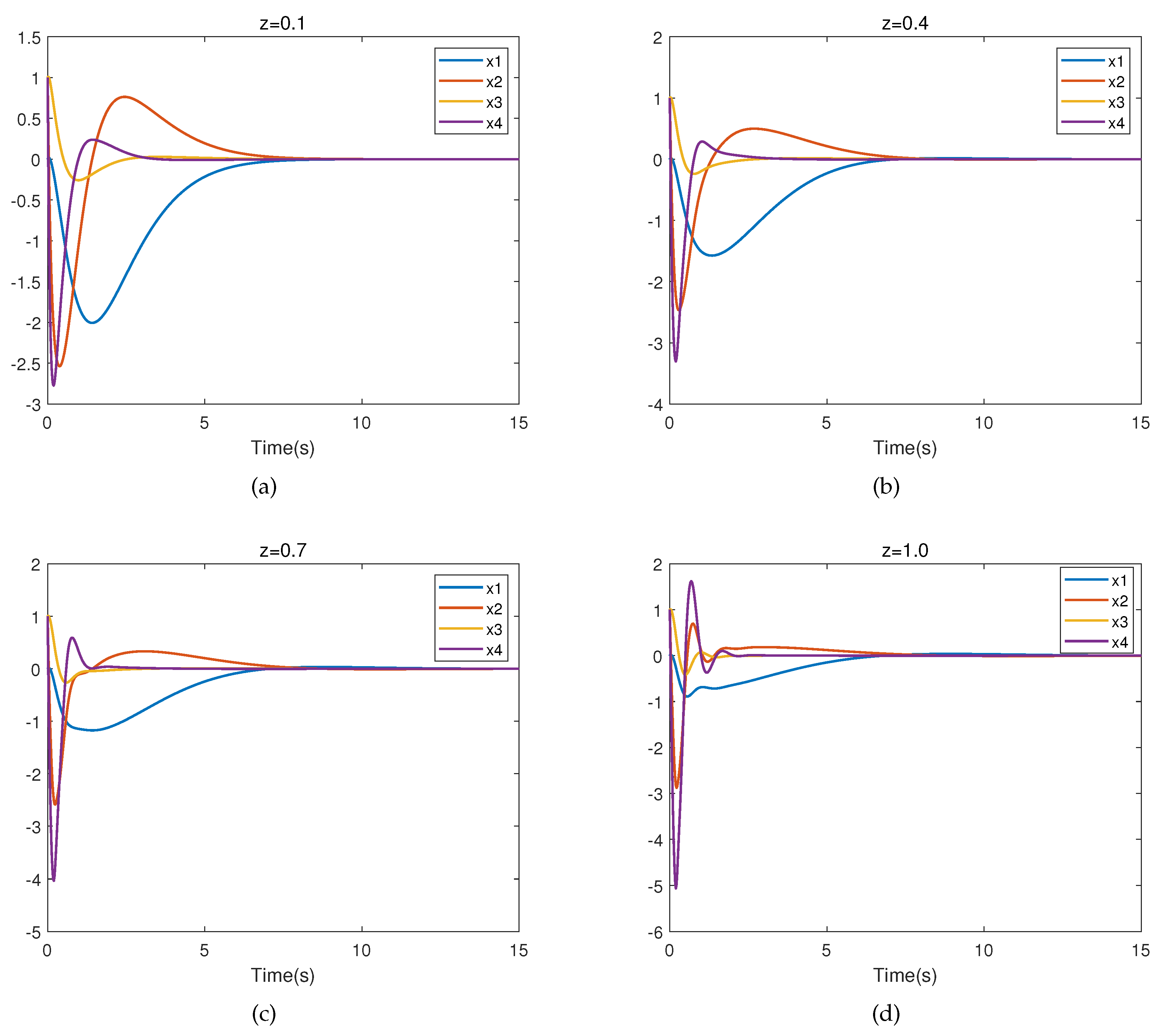
We also selected . Figure 10 presents the trajectory of the closed-loop system for different values of z.
7. Conclusions
In this paper, the robust control problem of the first-order IPS is studied. The linearization and nonlinear state-space representation are established, and an RL algorithm for the robust control of the IPS is proposed. The controller of the uncertain system is obtained using the method of online PI. The results thus obtained show that the error between the controller obtained using the RL algorithm and by directly solving ARE is very small. Moreover, the use of the RL algorithm can effectively circumvent the "curse of dimensionality.’’ Moreover, the algorithm can provide a controller that meets the requirements without the nominal matrix of the system being known. This improves the current state at which the robust control of the IPS relies excessively on the nominal matrix. In future research, we intend to take into consideration that the input matrix of the system also has uncertainty and extend the RL algorithm to more general systems.
Author Contributions
All the authors contributed equally to the development of the research.
Funding
This research was funded by the National Natural Science Foundation of China under Grant No. 61463002.
Acknowledgments
The authors thank to the Journal editors and the reviewers for their helpful suggestions and comments.
Conflicts of Interest
The authors declare no conflict of interest.
References
- Dai L. Strong decoupling in singular systems. Mathematical Systems Theory. 1989,22(1):275–2.
- Pal B, Chaudhuri B. Robust Control in Power Systems. Springer Science & Business Media.
- Liu L, Liu Y J, Tong S, et al. Relative threshold-based event-triggered control for nonlinear constrained systems with application to aircraft wing rock motion. IEEE Transactions on Industrial Informatics. 2022,18(2):911–921.
- Wang Z, She J, Wang F, et al. Further Result on Reducing Disturbance-Compensation Error of Equivalent-Input-Disturbance Approach. IEEE/ASME Transactions on Mechatronics. IEEE/ASME Transactions on Mechatronics (Early Access). [CrossRef]
- Yue D, Han QL, Lam J. Network-based robust H control of systems with uncertainty. Automatica. 2005,41(6):999–1007.
- Grasser F, D’arrigo A, Colombi S, Rufer AC. JOE: a mobile, inverted pendulum. IEEE Transactions on industrial electronics. 2002,49(1):107–114.
- Stephenson A. Memoirs and Proceedings of the Manchester Literary and Philosophical Society 52, 1–10. On a new type of dynamic stability. 1908.
- Housner GW. The behavior of inverted pendulum structures during earthquakes. Bulletin of the seismological society of America. 1963,53(2):403–417.
- Wang JJ. Simulation studies of inverted pendulum based on PID controllers. Simulation Modelling Practice and Theory. 2011,19(1):440–449.
- Prasad LB, Tyagi B, Gupta HO. Optimal Control of Nonlinear Inverted Pendulum System Using PID Controller and LQR: Performance Analysis Without and With Disturbance Input. International Journal of Automation and Computing. 2014,11:661–670.
- Li D, Chen H, Fan J, Shen C. A novel qualitative control method to inverted pendulum systems. IFAC Proceedings Volumes. 1999,32(2):1495–1500.
- Kwon T, Hodgins JK. Momentum-Mapped Inverted Pendulum Models for Controlling Dynamic Human Motions. ACM Transactions on Graphics (TOG). 2017,36(1):1–14.
- Yamakawa T. Stabilization of an inverted pendulum by a high-speed fuzzy logic controller hardware system. Fuzzy sets and Systems. 1989,32(2):161–180.
- Huang CH, Wang WJ, Chiu CH. Design and implementation of fuzzy control on a two-wheel inverted pendulum. IEEE Transactions on Industrial Electronics. 2010,58(7):2988–3001.
- Su X, Xia F, Liu J, Wu L. Event-triggered fuzzy control of nonlinear systems with its application to inverted pendulum systems. Automatica. 2018,94:236–248.
- Nasir ANK, Razak AAA. Opposition-based spiral dynamic algorithm with an application to optimize type-2 fuzzy control for an inverted pendulum system. Expert Systems with Applications. 2022,195:116661.
- Wai RJ, Chang LJ. Adaptive stabilizing and tracking control for a nonlinear inverted-pendulum system via sliding-mode technique. IEEE Transactions on Industrial Electronics. 2006,53(2):674–692.
- Huang J, Guan ZH, Matsuno T, Fukuda T, Sekiyama K. Sliding-mode velocity control of mobile-wheeled inverted-pendulum systems. IEEE Transactions on robotics. 2010,26(4):750–758.
- Jung S, Kim SS. Control experiment of a wheel-driven mobile inverted pendulum using neural network. IEEE Transactions on Control Systems Technology. 2008,16(2):297–303.
- Yang C, Li Z, Li J. Trajectory planning and optimized adaptive control for a class of wheeled inverted pendulum vehicle models. IEEE Transactions on Cybernetics. 2012,43(1):24–36.
- Yang C, Li Z, Cui R, Xu B. Neural network-based motion control of an underactuated wheeled inverted pendulum model. IEEE Transactions on Neural Networks and Learning Systems. 2014,25(11):2004–2016.
- Feng Lin and A. W. Olbrot, "An LQR approach to robust control of linear systems with uncertain parameters," Proceedings of 35th IEEE Conference on Decision and Control, Kobe, Japan, 1996, pp. 4158-4163 vol.4. [CrossRef]
- Lin F, Brandt RD. An optimal control approach to robust control of robot manipulators. IEEE Transactions on robotics and automation. 1998,14(1):69–77.
- Lin F. An optimal control approach to robust control design. International journal of control. 2000,73(3):177–186.
- Bellman R. Dynamic programming. Science. 1966,153(3731):34–37.
- Neustadt LW, Pontrjagin LS, Trirogoff K. The mathematical theory of optimal processes. Interscience, 1962.
- Powell WB. Approximate Dynamic Programming: Solving the curses of dimensionality. 703. John Wiley & Sons, 2007.
- Li H, Liu D. Optimal control for discrete-time affine non-linear systems using general value iteration. IET Control Theory & Applications. 2012,6(18):2725–2736.
- Wei Q, Liu D, Lin H. Value iteration adaptive dynamic programming for optimal control of discrete-time nonlinear systems. IEEE Transactions on cybernetics. 2015,46(3):840–853.
- Tesauro G. TD-Gammon, a self-teaching backgammon program, achieves master-level play. Neural computation. 1994,6(2):215–219.
- Crites R, Barto A. Improving elevator performance using reinforcement learning. Advances in neural information processing systems. 1995,8.
- Zhang W, Dietterich T. High-performance job-shop scheduling with a time-delay TD (λ) network. Advances in neural information processing systems. 1995,8.
- Singh S, Bertsekas D. Reinforcement learning for dynamic channel allocation in cellular telephone systems. Advances in neural information processing systems. 1996,9.
- Maja J M. Reward Functions for Accelerated Learning. In: Cohen WW, Hirsh H. , eds. Machine learning proceedings 1994, 1 ed., Morgan Kaufmann, 1994,181–189.
- Doya K. Reinforcement learning in continuous time and space. Neural computation. 2000,12(1):219–245.
- Krstic M, Kokotovic PV, Kanellakopoulos I. Nonlinear and adaptive control design. John Wiley & Sons, Inc., 1995.
- Ioannou P, Fidan B. Adaptive Control Tutorial, vol. 11 of Advances in Design and Control. SIAM, Philadelphia, Pa, USA,. 2006.
- Åström KJ, Wittenmark B. Adaptive control. Courier Corporation, 2013.
- Vrabie D, Pastravanu O, Abu-Khalaf M, Lewis FL. Adaptive optimal control for continuous-time linear systems based on policy iteration. Automatica. 2009,45(2):477–484.
- Xu D, Wang Q, Li Y. Adaptive optimal control approach to robust tracking of uncertain linear systems based on policy iteration. Measurement and Control. 2021, 54(5-6): 668-680.
- Xu D, Wang Q, Li Y. Optimal guaranteed cost tracking of uncertain nonlinear systems using adaptive dynamic programming with concurrent learning. International Journal of Control, Automation and Systems. 2020,18(5):1116–1127.
- Kleinman D. On an iterative technique for Riccati equation computations. IEEE Transactions on Automatic Control. 1968,13(1):114–115.
- Abu-Khalaf M, Lewis FL. Nearly optimal control laws for nonlinear systems with saturating actuators using a neural network HJB approach. Automatica. 2005,41(5):779–791.
Figure 1.
Inverted pendulum system diagram.
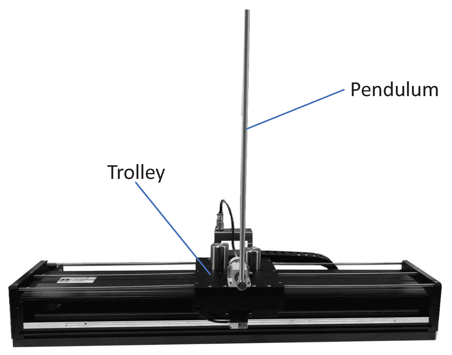
Figure 2.
First-order inverted pendulum physical model.
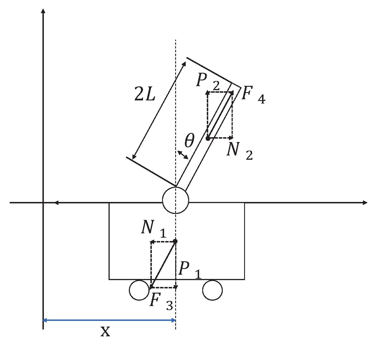
Figure 3.
Force analysis of the trolley.
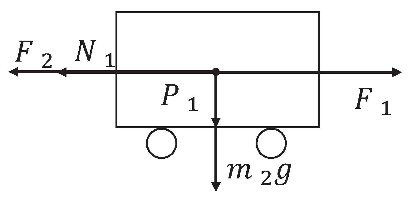
Figure 4.
Force analysis of the pendulum.
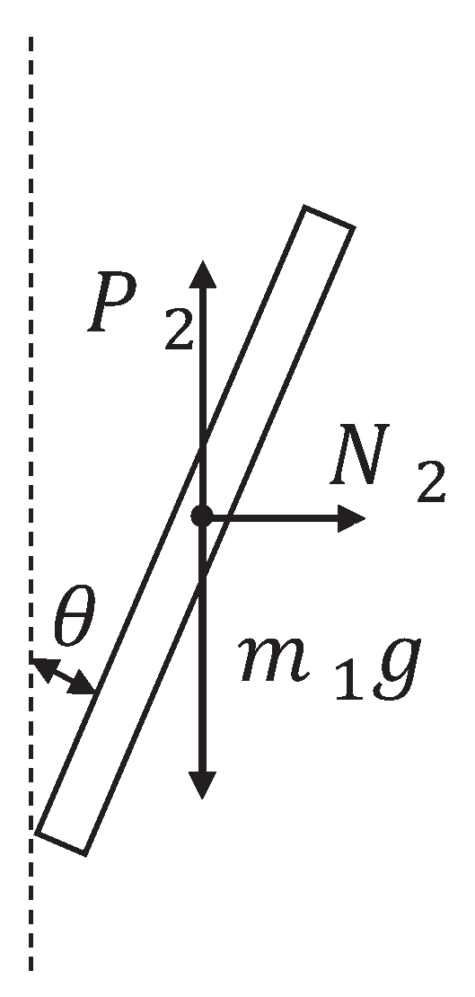
Figure 5.
Control signal u of the linearized system.
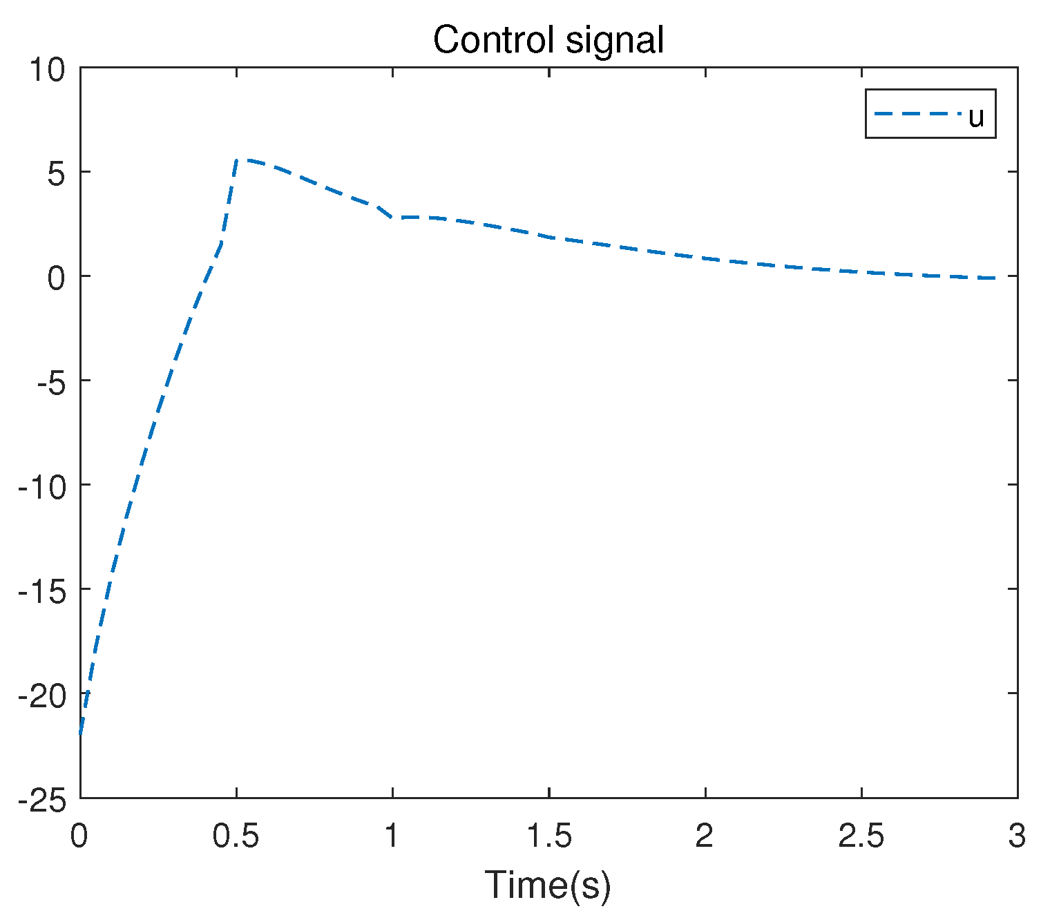
Figure 6.
S-matrix iterative process of the linearized system.
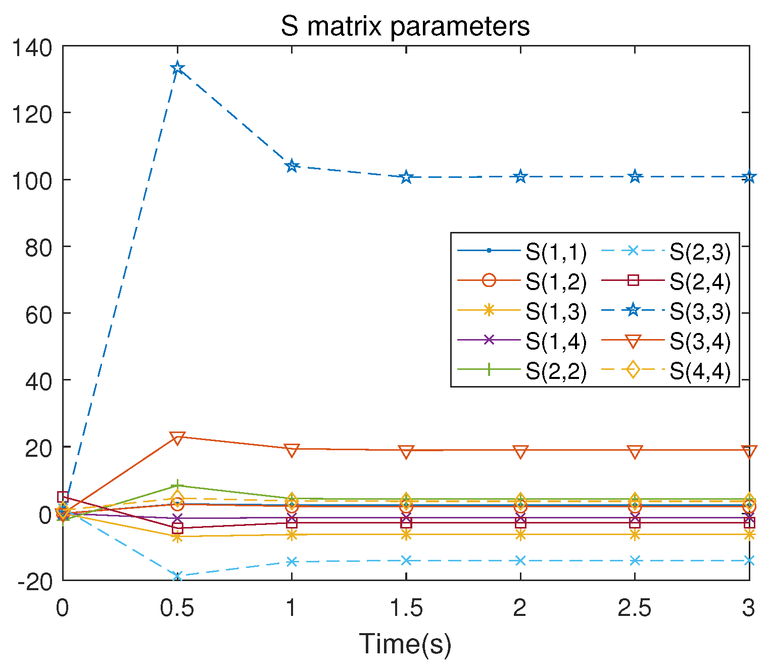
Figure 7.
Trajectory of closed-loop linearized system.
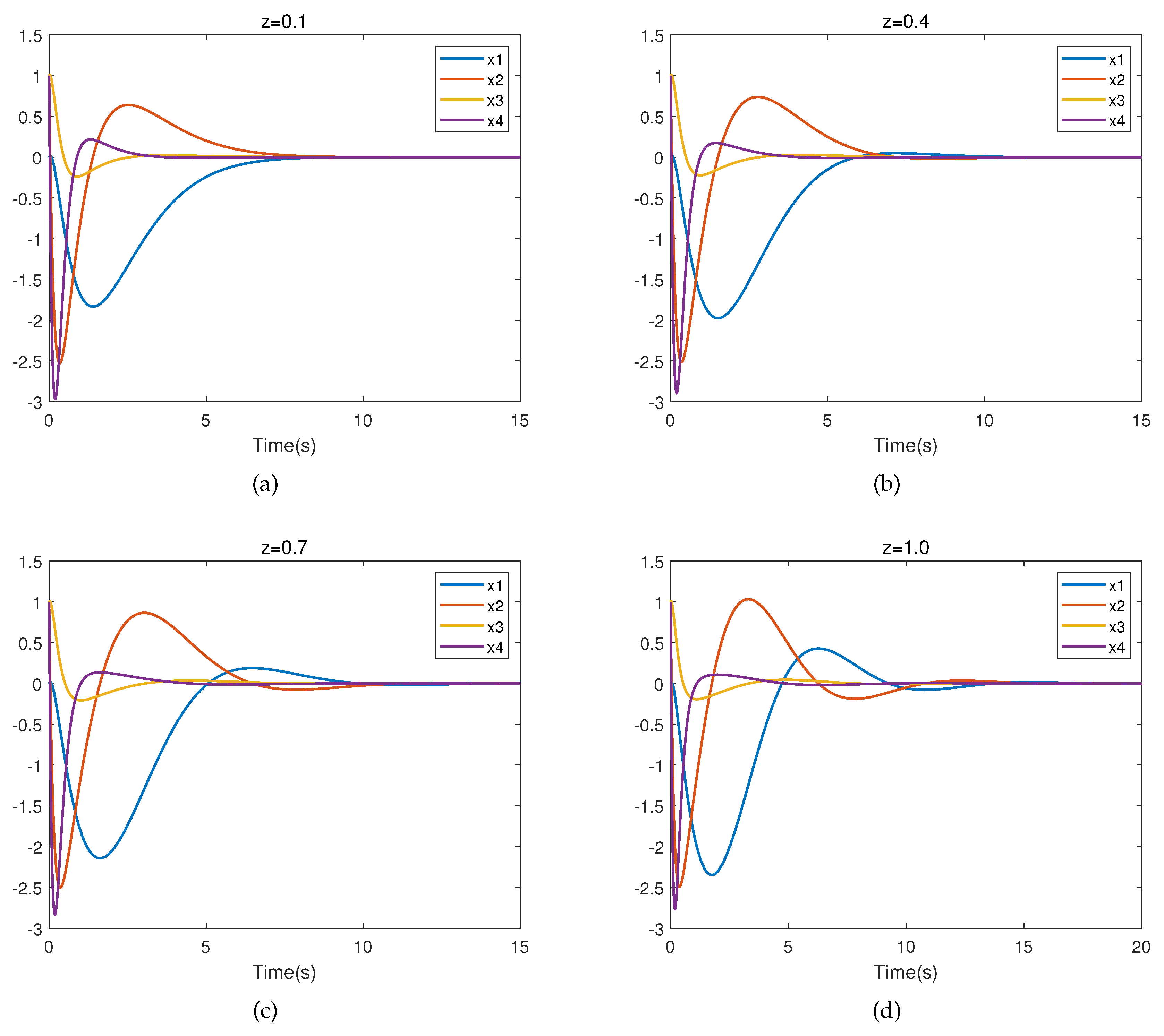
Figure 8.
Control signal u of the nonlinear system.
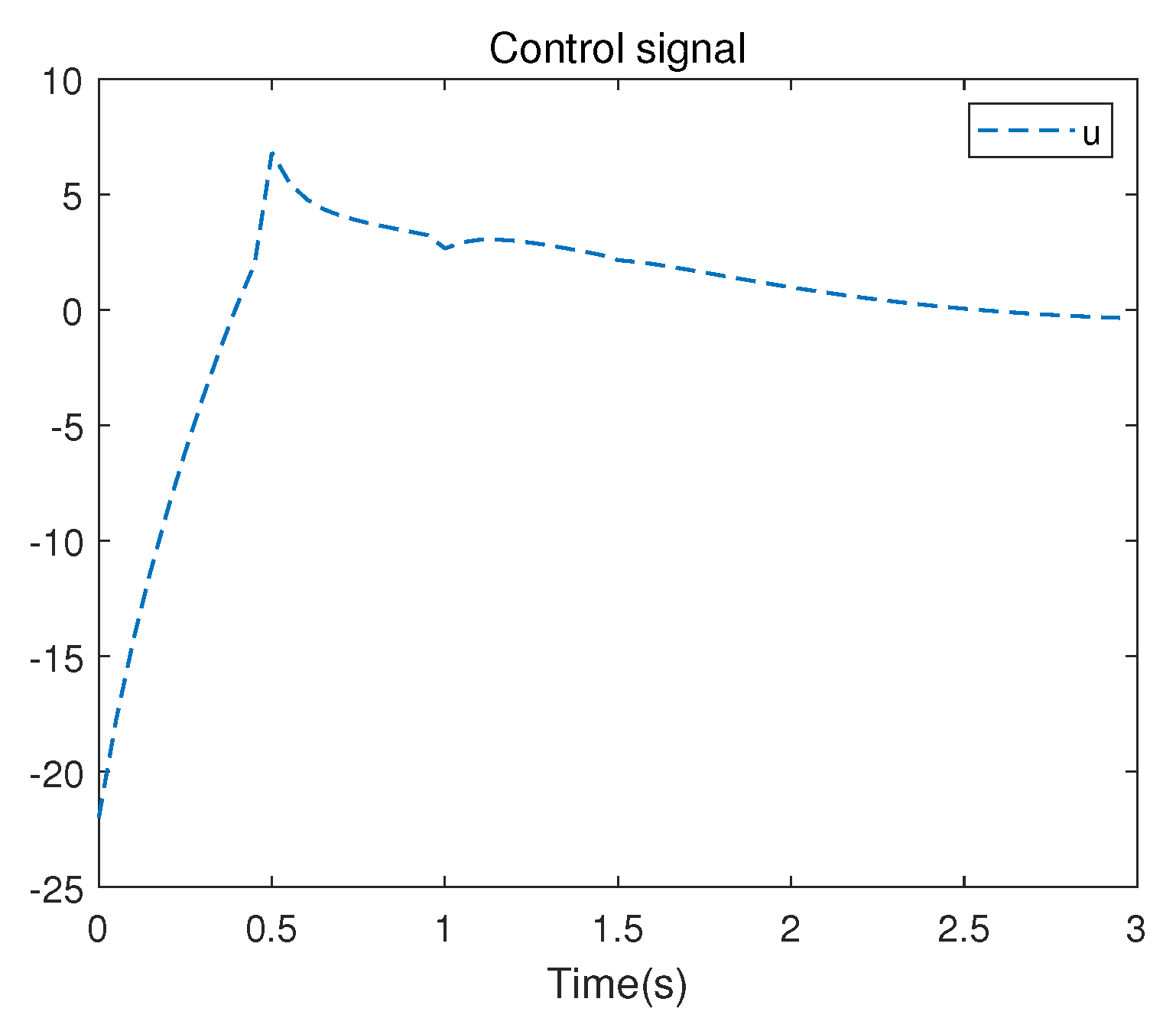
Figure 9.
S-matrix iterative process of the nonlinear system.
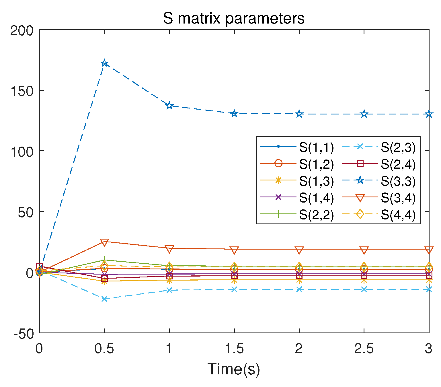
Figure 10.
Trajectory of closed-loop nonlinear system.
Disclaimer/Publisher’s Note: The statements, opinions and data contained in all publications are solely those of the individual author(s) and contributor(s) and not of MDPI and/or the editor(s). MDPI and/or the editor(s) disclaim responsibility for any injury to people or property resulting from any ideas, methods, instructions or products referred to in the content. |
© 2023 by the authors. Licensee MDPI, Basel, Switzerland. This article is an open access article distributed under the terms and conditions of the Creative Commons Attribution (CC BY) license (http://creativecommons.org/licenses/by/4.0/).
Copyright: This open access article is published under a Creative Commons CC BY 4.0 license, which permit the free download, distribution, and reuse, provided that the author and preprint are cited in any reuse.


