About Space Harmonics Effects on Performances of Linear Induction Motors: Modelization and Characterization

This article presents the impact analysis of space harmonics (SH) presence on a single-sided three-phase linear induction motor, along with a comprehensive parametric investigation. The presence of SH often reduces the LIM performances. The electromagnetic phenomena are governed by Maxwell's equations associated with equivalent circuit modelling. The chosen mathematical model uses 2D formulation with magnetic vector potential A. The model implementation is performed with finite element method on Gmsh-GetDP free platform. The electromagnetic thrust is calculated in current excitation case by a numerical model (FEM) with and without term generating SH in order to highlight the effect of SH. The adaptation to voltage supply operation is obtained by equivalent electric circuits (EEC), through calculation of the operational impedance. The main objective of the study consists in a comparative exploration of SH presence using two numerical models (single and multi-harmonics), and an assessment of parameters effect on space harmonic presence and various machine characteristics such as thrust, efficiency, and power factor. The motor’s characteristics (ie: thrust, efficiency and power factor) strongly depend on parameters such as the pole pair number and conductivity. Improving the operation and maximizing the performances of such a machine for a given specification requires the use of optimization algorithms.

Keywords:

Subject: Engineering - Electrical and Electronic Engineering

1. Introduction

Linear motors have been used in rail transport and in many industrial applications. Compared to other types, the single-sided linear induction motor can be used because of its simplicity and low construction cost, they are widespread and meet the industry’s requirements. It is therefore not at all surprising that it is still the subject of much research aiming to improve its modeling and optimizing its design. Despite its manufacture and implementation simplicity, the modeling and calculation of different quantities of the linear induction motor are not easy tasks. This is mainly due to the magnetic field which contains a continuous spectrum of space harmonics [1], and the non-linear character of materials. The requirement for precision, within the design process requires the use of accurate numerical methods [2,3,4].

In the design of a linear three-phase induction motor, we are generally confronted to the choice issue of the physical and geometrical parameters [5]. It is therefore essential to go through electromagnetic modeling, using field theory to develop equations that governs the linear induction motor [6,7].

In a classical rotating induction motor, one tries to produce a magnetic field owning only one space harmonic. In contrast with this, the condition cannot be obtained in a linear induction motor (LIM) which presents a continuous spectrum of space harmonics [1,8]. Space harmonics (SH) generally have a negative effect on the machine, reducing speed, efficiency and power factor and increasing losses, and machine heating. Research works on this question evoke often the SH problem without studying the problem itself [5,6]. Few works deal with this problem; rare references have tried to treat and reduce the effects of space harmonics by designing specific windings, modifying the geometry of the machine [9,10], position of the slots, frequency and complex phasors of the currents [8]. On the other hand, this issue has been well studied in the case of rotating machines [11,12,13].

A numerical program using finite element method can be used to model the electromagnetic behavior of the machine [14]. Assumptions can be made to consider a “perfect” sinusoidal travelling wave in the air-gap such in rotating induction machine by introducing the slip on the conductivity of the secondary. This is so-called single space harmonic model. However, due to the non-periodic geometry of the stator armature, the air-gap flux density is not periodic. Considering the exact formulation of eddy currents in the secondary by introduction the convective term

v \times B

considers fully the non-periodic behavior of the device and lead to more accurate results. Free Finite element software platform Gmsh-GetDP [15] is used to perform electromagnetic simulation. Connection to equivalent electrical circuit allows to deal with operation at imposed voltage supply that gives classical performances according to the speed of the secondary [16].

First, the thrust according to the speed generated by the LIM in real case taking in account the term responsible of SH presence is compared to the ideal case. Effect study of different parameters such as the pair pole number

(p)

and the conductivity

(σ)

on the (SH) presence are done in order to show those reducing and those accentuating the effect. The LIM thrust, power factor and efficiency are then studied according to the important parameters.

2. Linear Induction Motor Modeling

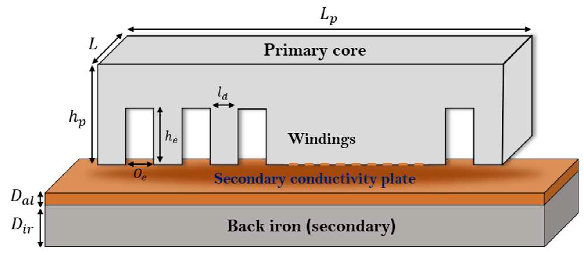
A schematic representation (Figure 1) illustrate a linear induction motor of

N_{e}

primary slots wounded to obtain

p

pole pairs winding. The secondary often composed by aluminum conductive and back-iron plates, which takes the place of the rotor in rotating induction machines.

A kind of characteristic speed

v_{s}

is defined as follows:

v_{s} = L f / p

where:

L

is the characteristic length attached to the LIM, which represents the total armature length.

f

is the supply frequency.

The primary moves at a speed v and a relative speed (

v_{r} = v / v_{s}

) is introduced. The product

L f

represents in a way, the synchronous speed

v_{s}

of a periodic motor with period. The quantities and the results bellow are studied and given according to the relative speed

v_{r}

The simplified model considers single space harmonic of the magnetic vector potential

(A)

assumed sinusoidal. The slip

s

is introduced as for rotating induction machines. Two-dimensional time harmonic formulation using magnetic vector potential is adopted for field calculation.

Model 1: single-harmonic

This model considers that the air-gap flux density is periodic and owns one space harmonic, neglecting the effect of all space harmonics. Equation (1) is to be solved by FEM, where the conductivity of the secondary is multiplied by the slip

s = 1 - v_{r}

as for induction machines:

\nabla . (\frac{1}{μ} \nabla A_{z}) = - J_{s} + σ j s ω A_{z}

(1)

b.: Model 2: multi-harmonic

In this model, air-gap flux density harmonics are considered as they are created by the stator winding. A Lagrangian formulation allows to express field equations line a frame of references linked to the stator armature. Due to the smooth geometry of the secondary, no diffraction occurs and therefore all the physical quantities have the same time frequency [17,18]. The eddy currents in the secondary (conductive plate) are due to movement (

v \times B)

and transformation

(\frac{d}{d t})

term. In 2D time harmonic formulation, yields:

\nabla . (\frac{1}{μ} \nabla A_{z}) = - J_{s} + σ (j ω A_{z} + v_{x} \frac{\partial A_{z}}{\partial x})

(2)

where

J_{s}

is the current density in the slots due to the stator currents.

3. 2d Finite Element Modelling

Two-dimensional finite element modeling is used to solve the two formulations models 1 and 2 which governs the electromagnetic phenomenon given by magnetic vector potential

A

. Free software Gmsh-GetDP is chosen to implement the two formulations issued from Model 1 and Model 2. The interesting idea is that the two models can be written in the same formulation by setting the parameters to:

Model 1:

v = 0

and

σ = s . σ_{O}

Model 2:

v = v_{x}

and

σ = σ_{O}

This is highlighted in the following screenshot of the formulation part of the code.

In the Model 1, the filed equation is quit standard Poisson’s equation usually solved in electrical machines. The stiffness matrix is symmetrical definite positive. The storage of the matrix needs the upper non-zero terms and the diagonal. The resolution of the final system is easy and fast. Many resolution methods can be used. The case of Model 2, is quite different. Due to the convective term

v . \nabla A

, the stiffness matrix generated with the formulation is not symmetrical. The storage of the whole matrix is needed. Therefore, the resolution time (CPU) is much higher than for Model 1. Especially for high values that lead to high values of magnetic Reynolds number

R_{m} = μ σ v_{x} L_{O}

that leads to numerical perturbations if the characteristic length

L_{0}

is too high. The mesh size must be adapted and refined so that these numerical perturbations vanishes.

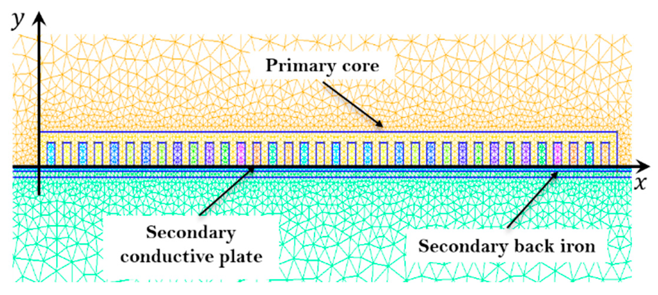
The triangular elements fit to any two-dimensional geometric configuration, which allows a simple discretization of the device. The mesh generated by the finite element program with the Gmsh software uses a triangular linear element mesh that is refined in the regions that need accuracy and wide in the other regions as shown in Figure 2.

The problem is solved using GetDP software to perform the implementation of the models.

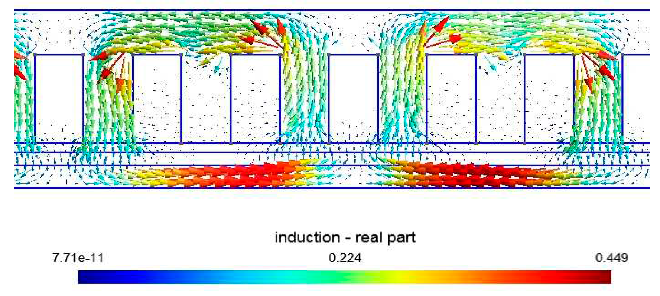
Figure 3 shows the representation of the magnetic flux density vector

B

derived from the calculated magnetic potential vector

A

(Eq. 3) in a part of the motor in each node of the mesh. It can be seen that the magnetic circuit channels the flux lines.

The data (Table 1) of each region for both, geometrical (dimensions) and physical (permeability

μ

and conductivity

σ

) properties of the studied device are introduced.

3.1. Current Density Source Calculation

To calculate the magnetic field and eddy current distribution in each region, the primary current density in the slots of a two-pole single-layer three phase winding is defined by a connection matrix

C_{0}

that links the phase currents and the stator slots. The expression given below is related to one pole pair and can be duplicated

p

times for a

p

poles pairs winding to obtained the whole connection matrix

C

C_{0} = [\begin{matrix} 1 & 0 & 0 \\ 0 & 1 & 0 \\ 0 & 0 & - 1 \end{matrix} \begin{matrix} - 1 & 0 & 0 \\ 0 & - 1 & 0 \\ 0 & 0 & 1 \end{matrix}]

(3)

when the single-layer winding machine is supplied by sinusoidal three phase currents, the ampere-turns

(N I)

in the slots can be calculated by:

{(N I)}_{k} = N_{t} C [\begin{matrix} I_{a} \\ I_{b} \\ I_{c} \end{matrix}]; k = 1 . . N_{e}

(4)

where

N_{t}

is the number of turns per slot and

I_{a}, I_{b}, I_{c}

denotes the phase currents.

The stator current density

J_{s} (x, y)

in the slots and used in (1) and (2), is defined as the sum of slot current densities due to the ampere-turns in the slots.

4. Connection with Equivalent Electric Circuit

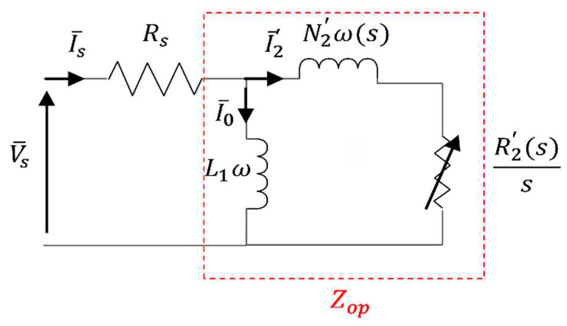
In this paper, a simplified equivalent electric circuit (EEC) is considered to evaluate the performances of the machines under a voltage supply [19,20]. Neglecting the iron losses and assuming the first harmonic hypothesis, the used EEC is shown on Figure 4.

where

-: R_s is the stator resistance which can be determined by classical analytical formula,
-: L₁ is the primary inductance (i.e., the magnetizing inductance),
-: N’₂(s) is the leakage inductance expressed in the secondary frame which depends on the slip,
-: R’₂(s) is the equivalent resistance expressed in the secondary frame which depends on the slip.

Finally,

Z_{o p}

is the equivalent operational impedance of the machine in the hypothesis of mono-harmonic model. Such model can be used in connection with single harmonic model (Model 1). In case of Model 2, no need to go in details for

Z_{o p}

. The most important thing is to determine the operational impedance and evaluate the stator current with the circuit model.

4.1. Voltage Supply And Electric Parameters Identification

The approach adopted for the calculation of the EEC parameters uses both FEM and analytical method presented in this paper [21]. When the machine is supplied with a three-phase voltage

{\bar{V}}_{s}^{a b c}

given by:

{\bar{V}}_{s}^{a b c} = V_{m}^{a b c} [1 e^{- j \frac{2 π}{3}} e^{j \frac{2 π}{3}}]

(5)

where

V_{m}^{a b c}

is the amplitude of the three-phase voltage.

The calculation of the operational impedance is performed as follows:

-: Calculate the phases fluxes ${\bar{φ}}^{a b c}$ by using magnetic vector potential in the slots and winding matrix.
-: Calculate the emfs: $\{{\bar{E}}^{a b c}\} = j ω_{s} \{{\bar{φ}}^{a b c}\}$
-: Calculate the impedances with ${\bar{Z}}_{o p}^{a b c} = \frac{\{{\bar{E}}^{a b c}\}}{{\bar{I}}^{a b c}}$

This method has been widely used for the modelling of rotating induction machines even for single harmonic model or multiharmonic model [22]. The operational impedances for the three phases are equal due to the balance of the phases in conventional induction machines. The calculation can be performed one of the stator phases. However, in case of linear induction the imbalance of the phases requires to perform the calculations on the three phases. Indeed, the phases are not balanced, as well as the impedances and the stator currents that are shown below [23].

4.2. The Phase Currents

The stator phase currents

{\bar{I}}^{a b c}

for each value of the speed v can then be determined as follow:

{\bar{I}}_{s}^{a b c} = \frac{{\bar{V}}_{s}^{a b c}}{{\bar{Z}}_{o p}^{a b c} + {\bar{R}}_{s}^{a b c}}

(6)

The calculation of the stator currents with (6), allows to perform field calculation given by (1) and (2) for model 1 and model 2 respectively. This is the final right computation of field distribution in the machine for the considered speed at fixed voltage [24].

At this step, performances of the machine can be calculated either by field equation (force) or input power (input voltage and currents)

4.3. Force calculation

In the two-dimensional hypothesis, the magnetic potential vector

A

has a single component

A_{z}

oriented along the transverse axis

(O_{Z})

, and its value depends only on the

x

and

y

coordinates. The magnetic flux density is given by the gradient of

A

as follow

B = \nabla A_{z} = \frac{\partial A_{z}}{\partial y} e_{x} - \frac{\partial A_{z}}{\partial x} e_{y}

(7)

where

e_{x}

and

e_{y}

denote the unit vector in the cartesian references.

The tangential component

B_{x}

of magnetic flux density creates normal forces in the linear induction motor, whereas, the normal component

B_{y}

generates the motor thrust. In a 2D approximation, the global Lorenz force

F

is written as follows.

F = L_{z} \iint_{S}^{} J_{v} \times B d s

(8)

where

L_{z}

is the length of the machine in

z

-direction. In the case of time harmonic formulation, the complex representation of electromagnetic quantities is used. The average values of tangential and normal components of the force (

F_{x}

and

F_{y}

) are given by the following formulas (9.a and 9.b)

F_{x} = L_{z} R \iint_{S}^{} J_{z} B_{y}^{*} d s

(9.a)

F_{y} = - L_{z} R \iint_{S}^{} J_{z} B_{x}^{*} d s

(9.b)

R

denotes: "real part of"

4.4. Power Factor And Efficiency

The knowledge of the input power from circuit equation and the calculation of the losses in the stator

P_{j s}

winding and secondary

P_{j r}

makes it possible to evaluate the efficiency

η

and the power factor

P_{f}

by:

η = \frac{F_{x} . v_{x}}{F_{x} . v_{x} + P_{j s} + P_{j r}} = \frac{R ({\bar{V}}_{s}^{a b c} * {}^{t}{{\bar{(I}}_{s}^{a b c})}^{*}) - P_{j s} - P_{j r}}{R ({\bar{V}}_{s}^{a b c} * {}^{t}{{\bar{(I}}_{s}^{a b c})}^{*})}

(10)

P_{f} = \frac{R ({\bar{V}}_{s}^{a b c} * {}^{t}{{\bar{(I}}_{s}^{a b c})}^{*})}{|{\bar{V}}_{s}^{a b c} * {}^{t}{{\bar{(I}}_{s}^{a b c})}^{*}|}

(11)

5. Results and Discussion

The LIM, with characteristics given in Table 1, is modeled by the FEM. First, the force-speed characteristic calculated with the two models are presented compared and discussed. In a second step, a parametric study is performed to highlight the effect of some parameters on output performances.

5.1. Illustration of Space Harmonics Effect

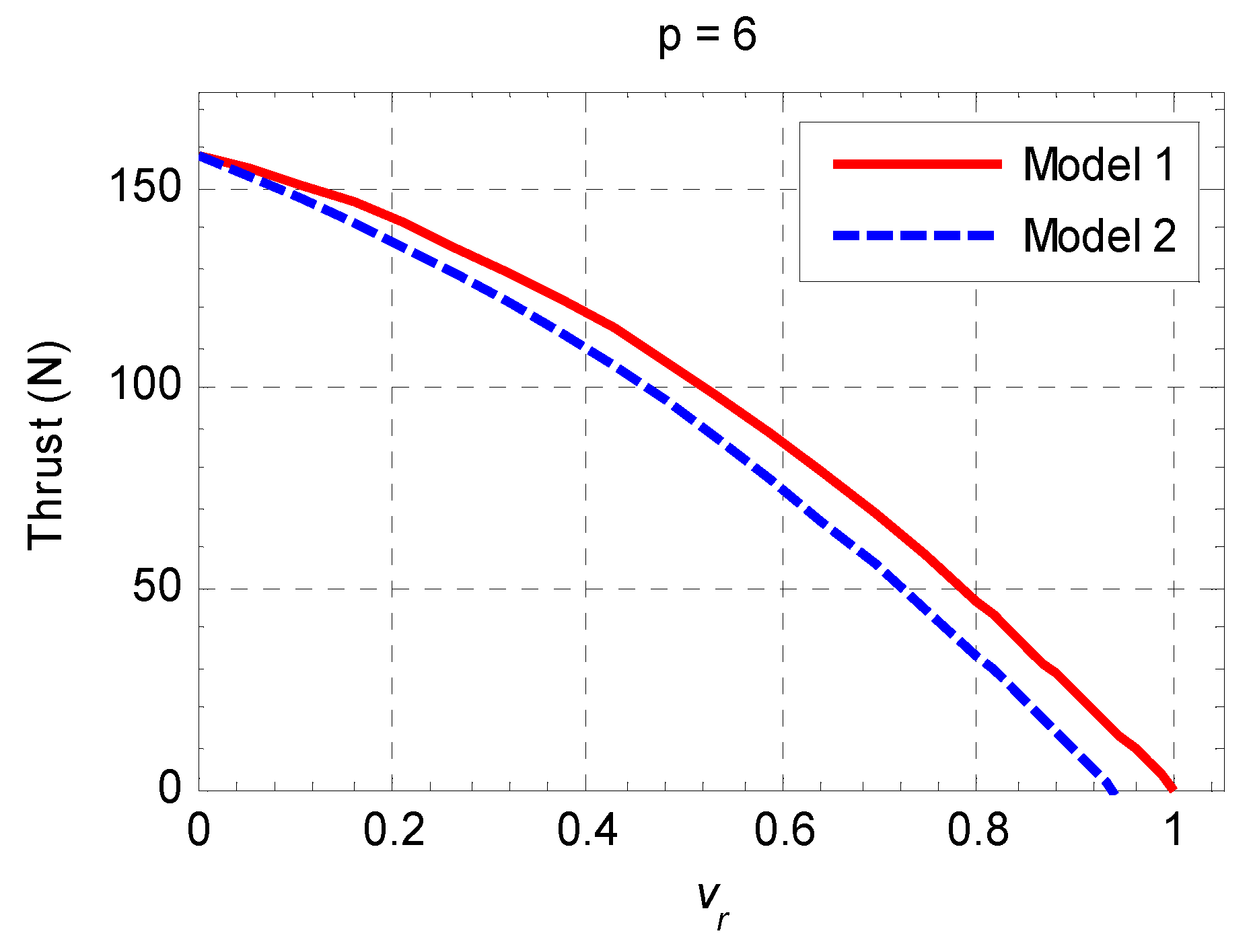
Figure 5 illustrates the difference between force-speed curves obtained by respectively the single-harmonic and multi-harmonic models in case of 12 pole winding (

p = 6)

. The force decreases with the relative speed

v_{r}

and drops to zero at synchronous speed (

v_{r} = 1)

. In case of model 2, the force is lower due to SH presence effect and the force vanishes to zero at a speed bellow synchronous speed

v_{r} = 1

. This behavior is coherent since the model 1 considers one harmonic and uses the slip parameter whereas multiharmonic model accounts for the presence of all space harmonics. Some of them create a negative force so that the total force is zero below synchronous speed. For this model, we talk about synchronous speed of the fundamental wave, but in practice, there are an infinity of waves travelling at different speeds in the two directions.

5.2. Impact Of Pole Number

In the following, all the results are presented according to the relative speed

v_{r} = L f / p

which means that for different pole numbers, the reference speed changes with the inverse of pole number.

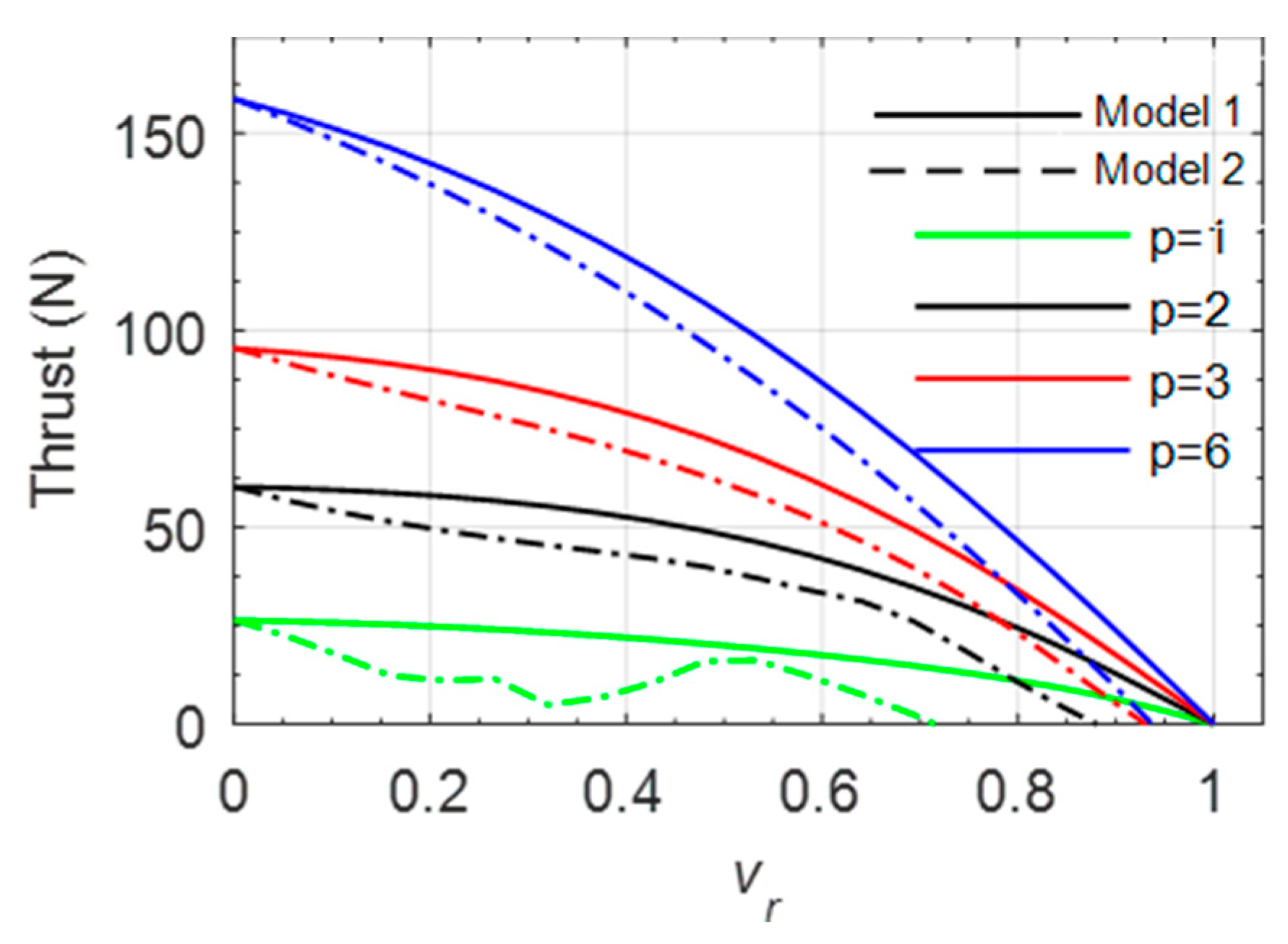
The case presented on Figure 5 is optimist because it considers 6 pole pairs. The end-effects are supposed to be low and negligible. If the number of poles decreases, end-effect increase and the distortion of the air-gap flux density is important. Figure 6 presents the Force-speed characteristics for the same machine with different pole numbers obtained with the two models. The geometry of the stator is conserved. The winding changes, and the number of slots per pole and per phase changes from

q = 1

for

p = 6

q = 6

for 2-pole winding.

The force curves shown on Figure 6, decrease with the velocity form maximal force at standstill and vanishes to zero close to synchronous speed. The force obtained by model 1 is always higher than that obtained by model 2 because model 1 is optimist and do not consider harmonics. In addition, one can see that for

p = 1

the force speed characteristic has a very disturbed shape and very low values compared to the previsions of model 1.

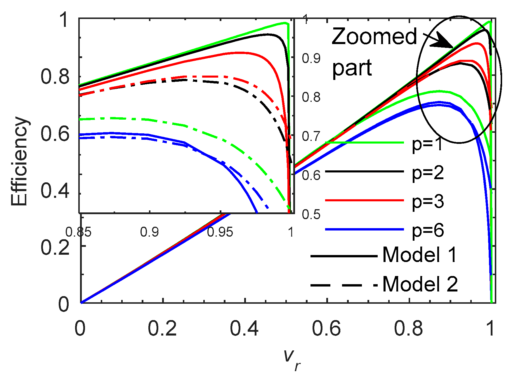
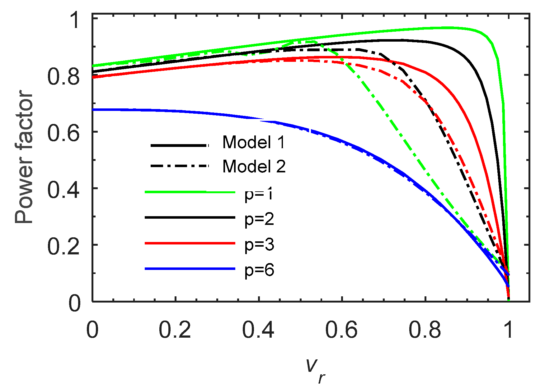
The consequence of the assumptions made by model 1 is that the performances are better in terms of force but also in terms of efficiency and power factor (Figure 7 and Figure 8). One can see that the shape of these curves is similar to those of induction machine and the behavior is correct. Power factor is low for high pole numbers as well as efficiency. Such results are to be taken with too much cautions because of the strong assumptions. Full model that considers space harmonics is required.

However, it can be seen that for high pole numbers (

p = 6

), the results given by the two models are quite similar. This means that if the pole number is too high, the end-effects become negligible and air-gap flux density presents a pseudo-sinusoidal shape. In this case, a single harmonic model could be sufficient to evaluate the machine performances.

Without SH presence (Model 1), the efficiency decreases with the pair poles number (Figure 7), whereas with SH presence (Model 2), the efficiency has a maximum value for

p = 3

and the lowest one for

p = 1

and

p = 6

(Figure 7).

Except for

p = 6

, where it decreases continuously, the power factor (Figure 8) increases with relative speed

v_{r}

, reaching a maximum and dropping at synchronous speed to 0.04 in the case without SH presence and to 0.1 in the case with SH presence. In the Model 1, the power factor has the maximum for

p = 1

and decrease according to the pole pairs number p, whereas in the Model 2, as for the efficiency, the maximum is obtained for

p = 3

working velocity near the synchronous speed.

5.3. Effect of Electrical Conductivity

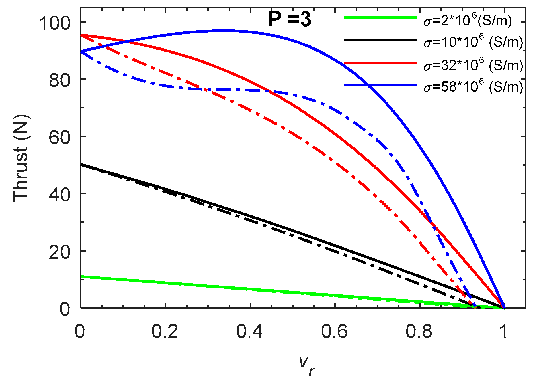
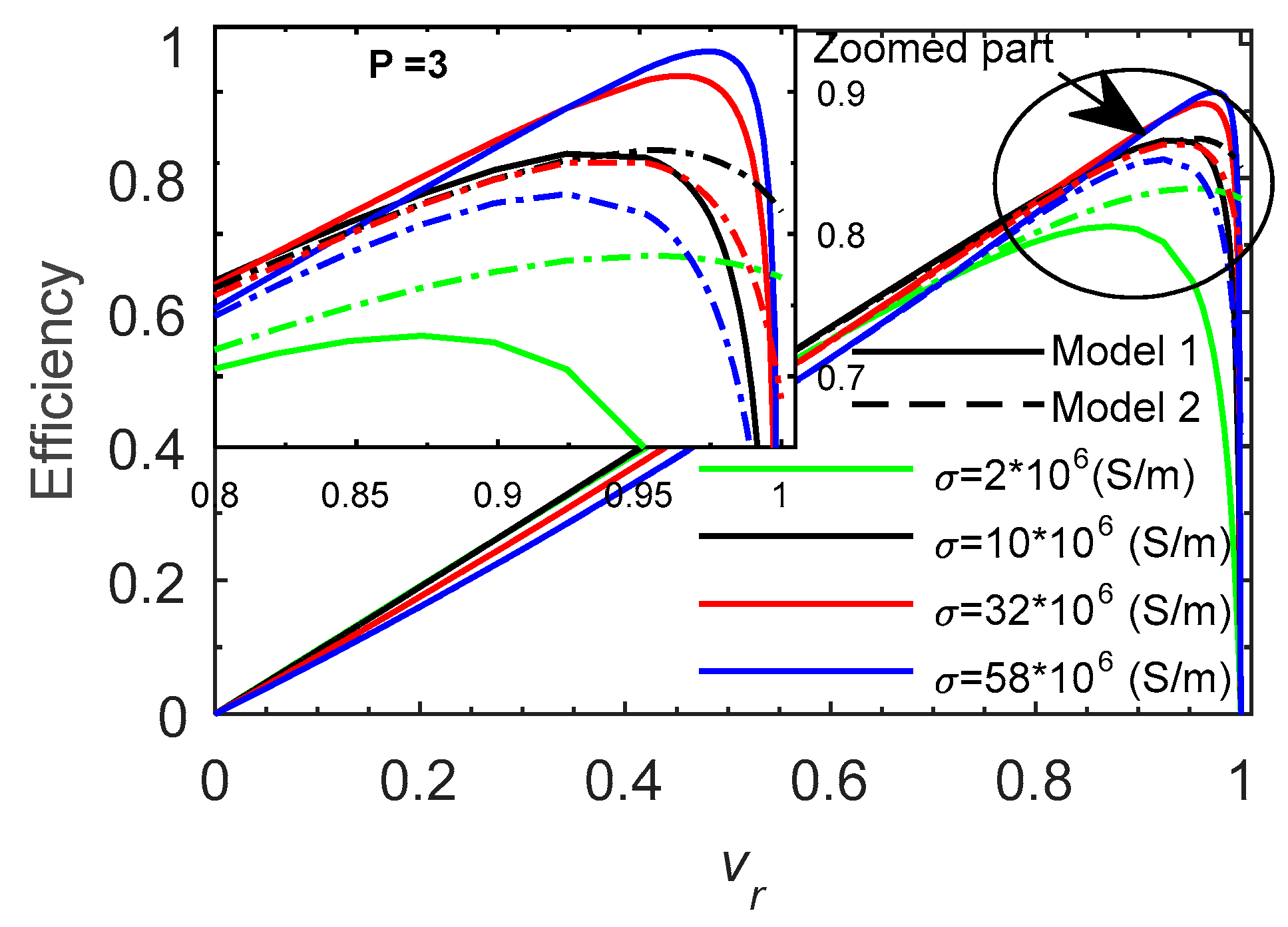
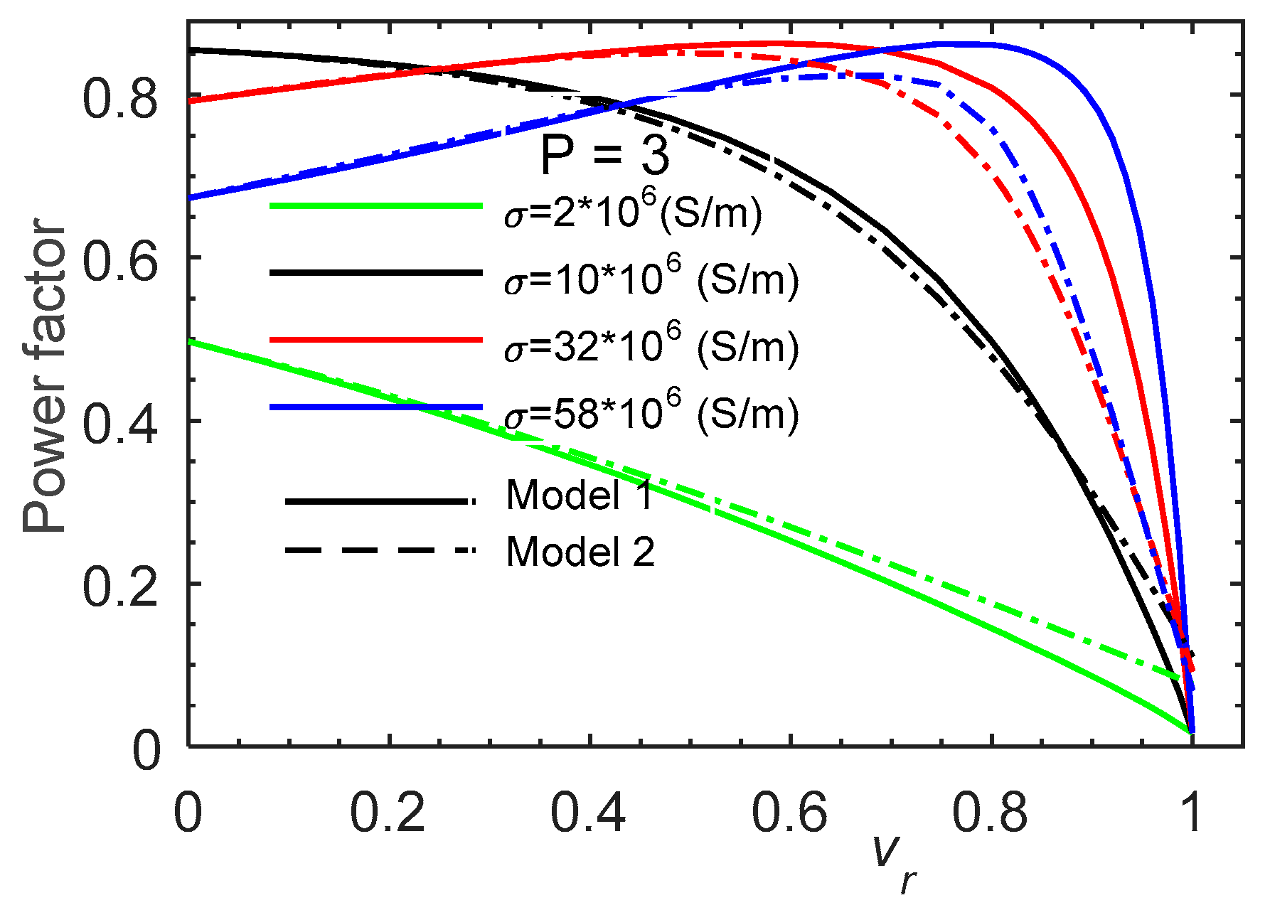
The electrical conductivity is also one property that affects the features of the LIM as shown in Figure 9, Figure 10 and Figure 11. The obtained curves have classical shapes with a maximal value that depends on the relative speed. The thrust (Figure 9) increases with the conductivity (iron, steel, aluminum and copper) and presents an optimal value such for rotating induction machines. It can be expected that for lower conductivities, the maximum values are reached for negative speeds that are not represented in these figures.

It is also seen that Model 2 gives shape of Force-speed curves below those given by model 1. The efficiency and the power factor (Figure 10 and Figure 11) have not linear behavior, the SH presence reduce generally them but this is not always the case.

At start-up and at low speed, the efficiency decreases with the conductivity in both models (1 and 2), while the power factor varies in a non-linear manner. The power factor lowest value is obtained for the lowest conductivity for iron

(2 * 10^{6} S / m)

, the maximum is obtained with steel

(10 * 10^{6} S / m)

and decreases with the other conductivities respectively Aluminum and Copper.

At work velocity

{(v}_{r} = 0.8 t o 1

), conversely at low speed, according to the conductivity, the efficiency increases in model 1 and the power factor increase in models 1 and 2 with good value for copper. While the efficiency in model 2 presents a good value for steel

(10 * 10^{6} S / m)

and Aluminum

(32 * 10^{6} S / m)

and decrease for copper and iron.

The general behavior of the external performances of the model are conform to the physical phenomena observed in induction machines. This model is fast and can easily be used in future design processes.

6. Conclusion

Single-harmonic and a multi-harmonics models are developed in Matlab and Gmsh-GetDP environment enabled a study of SH effects of a three-phase single sided linear induction motor. The electromagnetic thrust is calculated by FEM (model 1 and 2). The parameters’ behavior on the different characteristics of the machine are analyzed and discussed.

The multi-harmonic model shows that the space harmonics are not taken into a count the single-harmonic sinusoidal model, leading to significant errors.

The thrust increases with the pole pairs number, with the conductivity.

Space harmonics presence effect is related to the displacement speed

v_{r}

; it is absent or very weak at low speeds and significant near the synchronizing speed, thus cancelling the thrust before the synchronous speed and increase machine slip (s).

Space harmonics reduce the power factor and the efficiency witch have a complex nonlinear correlation with the pole pairs number, they increase with the electrical conductivity.

Increasing the pole pairs number

(p = 1 t o 6)

rise the speed, reduce the harmonics presence and makes the LIM behaving as an induction machine.

At work velocity

{(v}_{r} = 0.8 t o 1

), the machine presents a good power factor for aluminum and copper materials and a good efficiency for aluminum materials.

The machine parameters such as secondary conductivity and number of pairs poles phase play an important role in the performance of linear induction machines. Because of the complex nonlinear correlation between the machine parameters and the machine performance like speed, power factor and efficiency, it is difficult to choose directly the optimal parameters. Thus, to enhance the machine performances to obtain an optimal operation of such a machine for a given specification, it is necessary to use optimization techniques.

Author Contributions

Conceptualization A.B. (Aissa Bensehila) and A.B. (Athmane Bouzidi); methodology A.B. (Athmane Bouzidi) and N.T.; validation, A.B. (Aissa Bensehila) and A.B. (Athmane Bouzidi), writing—original draft preparation, A.B.(Aissa Bensehila) and A.B.(Athmane Bouzidi); writing—review and editing, N.T., A.B.(Athmane Bouzidi); supervision, N.T. and A.B.(Athmane Bouzidi); project administration, N.T. and. All authors have read and agreed to the published version of the manuscript.

Funding

This research received no external funding.

Conflicts of Interest

The authors declare no conflict of interest.

References

Palka, R.; Woronowicz, K. Linear Induction Motors in Transportation Systems. Energies 2021, 14, 2549. [Google Scholar] [CrossRef]
Woronowicz, K.; Safaee, A. A Novel Linear Induction Motor Equivalent-Circuit with Optimized End Effect Model. Can. J. Electr. Comput. Eng. 2014, 37, 34–41. [Google Scholar] [CrossRef]
Sari, M.; Ouazir, Y.; Mezani, S. New 2D Quasi-Analytical Computation of Eddy Currents in Axisymmetrical Problems: Application to Tubular Linear Induction Motor. IEEE Trans. Magn. 2023, 59, 1179–1183. [Google Scholar] [CrossRef]
Wu, S.; Lu, Q. Eddy Current Analysis and Optimization Design of the Secondary of the Linear Induction Motor with an Approximation and Prediction Method. IEEE Trans. Magn. 2021, 58, 1–5. [Google Scholar] [CrossRef]
Shiri, A.; Tessarolo, A. Normal Force Elimination in Single-Sided Linear Induction Motor Using Design Parameters. IEEE Trans. Transp. Electrification 2022, 8, 109–119. [Google Scholar] [CrossRef]
Lee, B. J.; Koo, D. H.; Cho, Y. H. Investigation of Linear Induction Motor According to Secondary Conductor Structure. IEEE Trans. Magn. 2009, 45, 2839–2842. [Google Scholar] [CrossRef]
Xing, F.; Kwon, B.-I. Design of a Rotary-Linear Motor with Unipolar SPM and Voice Coil Structure. IEEE Access 2020, 8, 150291–150300. [Google Scholar] [CrossRef]
Laporte, B.; Takorabet, N.; Vinsard, G. An Approach to Optimize Winding Design in Linear Induction Motors. IEEE Trans. Magn. 1997, 33, 1844–1847. [Google Scholar] [CrossRef]
Gieras, J. F.; Mews, J.; Splawski, P. Analytical Calculation of Electrodynamic Levitation Forces in a Special-Purpose Linear Induction Motor. IEEE Trans. Ind. Appl. 2011, 48, 106–116. [Google Scholar] [CrossRef]
Lv, G.; Zeng, D.; Zhou, T. Analysis of Secondary Losses and Efficiency in Linear Induction Motors with Composite Secondary Based on Space Harmonic Method. IEEE Trans. Energy Conv. 2017, 32, 1583–1591. [Google Scholar] [CrossRef]
Neto, L. M.; Camacho, J. R.; Salerno, C. H.; et al. Analysis of a Three-Phase Induction Machine Including Time and Space Harmonic Effects: The A, B, C Reference Frame. IEEE Trans. Energy Conv. 1999, 14, 80–85. [Google Scholar] [CrossRef]
Kindl, V.; Cermak, R.; Ferkova, Z.; et al. Review of Time and Space Harmonics in Multi-Phase Induction Machine. Energies 2020, 13, 496. [Google Scholar] [CrossRef]
Pereira, L. A.; Nicol, G.; Pereira, L. F. A.; et al. Effects of High-Order Space Harmonics on the Operation of Five-Phase Induction Machines Under Unbalance. ISA Trans. 2022, 131, 672–692. [Google Scholar] [CrossRef]
Bazghaleh, A. Z.; Choolabi, E. F. A New Approach for Non-Linear Time-Harmonic FEM-Based Analysis of Single-Sided Linear Induction Motor Incorporated with a New Accurate Method of Force Calculation. IEEE Trans. Magn. 2021, 57, 1. [Google Scholar] [CrossRef]
Dular, P.; Geuzaine, C. GetDP Reference Manual: The Documentation for GetDP, a General Environment for the Treatment of Discrete Problems, Jul. 20, 2019. [Online]. Available: http://getdp.info.
Gomes, D. R.; Chabu, I. E. A Novel Analytical Equivalent Circuit for Single-Sided Linear Induction Motors Considering Secondary Leakage Reactance. Energies 2023, 16, 1261. [Google Scholar] [CrossRef]
Lv, G.; Liu, Z.; Sun, S. Analysis of Torques in Single-Side Linear Induction Motor with Transverse Asymmetry for Linear Metro. IEEE Trans. Energy Conv. 2016, 31, 165–173. [Google Scholar] [CrossRef]
Takorabet, N. Computation of Force Density Inside the Channel of an Electromagnetic Pump by Hermite Projection. IEEE Trans. Magn. 2006, 42, 430–433. [Google Scholar] [CrossRef]
Lu, Q.; Li, L.; Zhan, J.; et al. Design Optimization and Performance Investigation of Novel Linear Induction Motors with Two Kinds of Secondaries. IEEE Trans. Ind. Appl. 2019, 55, 5830–5842. [Google Scholar] [CrossRef]
Xu, W.; Sun, G.; Wen, G.; et al. Equivalent Circuit Derivation and Performance Analysis of a Single-Sided Linear Induction Motor Based on the Winding Function Theory. IEEE Trans. Veh. Technol. 2012, 61, 1515–1525. [Google Scholar] [CrossRef]
Xu, W.; Hu, D.; Lei, G.; et al. System-Level Efficiency Optimization of a Linear Induction Motor Drive System. CES Trans. Electr. Mach. Syst. 2019, 3, 285–291. [Google Scholar] [CrossRef]
Boughrara, K.; Takorabet, N.; Ibtiouen, R.; Touhami, O.; Dubas, F. Analytical Analysis of Cage Rotor Induction Motors in Healthy, Defective, and Broken Bars Conditions. IEEE Trans. Magn. 2014, 51, 1–17. [Google Scholar] [CrossRef]
Lv, G.; Zhou, T.; Zeng, D. Influence of the Ladder-Slit Secondary on Reducing the Edge Effect and Transverse Forces in the Linear Induction Motor. IEEE Trans. Ind. Electron. 2018, 65, 7516–7525. [Google Scholar] [CrossRef]
Lee, B. J.; Koo, D. H.; Cho, Y. H. Investigation of Linear Induction Motor According to Secondary Conductor Structure. IEEE Trans. Magn. 2009, 45, 2839–2842. [Google Scholar] [CrossRef]

Figure 1. Generic design of LIM.

Figure 2. 2D mesh of linear induction motor of 36 slots.

Figure 3. Distribution of magnetic induction field 2D.

Figure 4. Condensed equivalent diagram of a linear induction.

Figure 5. Force-Speed characteristics.

Figure 6. Force-Speed characteristics for different pole numbers.

Figure 7. The efficiency according to

v_{r}

for different pole number.

Figure 7. The efficiency according to

v_{r}

for different pole number.

Figure 8. Power factor according to

v_{r}

for different pole numbers.

Figure 8. Power factor according to

v_{r}

for different pole numbers.

Figure 9. Thrust speed characteristic for different conductivity values.

Figure 10. The efficiency versus

v_{r}

for different conductivity values.

Figure 10. The efficiency versus

v_{r}

for different conductivity values.

Figure 11. Power factor versus

v_{r}

for different conductivity values

Figure 11. Power factor versus

v_{r}

for different conductivity values

Table 1. Design parameters of the Lim.

Designation	Symbol	Value
Inductor length	$L_{p}$	$730 m m$
Rail thickness	$D_{a l}$	$3 m m$
Air-gap length	$g$	$2 m m$
Relative permeability of the Back iron	$μ_{r}$	$4416 H / m$
Relative permeability of the primary armatures	$μ_{a r}$	$4416 H / m$
Number of turns	$n_{s}$	$100$
Number of phases	$m$	$3$
Number of pole pairs	$P$	$6$
Electric conductivity of plate (Aluminum)	$σ$	$32,3 . 10^{6} S / m$
Number of slots	$N e$	$36$
Frequency	$f$	$50 H z$
Phase current	$I_{a b c}$	$1 A$
Phase voltage	$V_{a b c}$	$230 V$
Thickness of back iron	$D_{i r}$	$5 m m$
Width of slot	$L_{d}$	10 $m m$

Disclaimer/Publisher’s Note: The statements, opinions and data contained in all publications are solely those of the individual author(s) and contributor(s) and not of MDPI and/or the editor(s). MDPI and/or the editor(s) disclaim responsibility for any injury to people or property resulting from any ideas, methods, instructions or products referred to in the content.

© 2023 by the authors. Licensee MDPI, Basel, Switzerland. This article is an open access article distributed under the terms and conditions of the Creative Commons Attribution (CC BY) license (http://creativecommons.org/licenses/by/4.0/).

Copyright: This open access article is published under a Creative Commons CC BY 4.0 license, which permit the free download, distribution, and reuse, provided that the author and preprint are cited in any reuse.

MDPI Initiatives

Important Links

Choose an area of interest and we will send you notifications of new preprints at your preferred frequency.

Disclaimer

About Space Harmonics Effects on Performances of Linear Induction Motors: Modelization and Characterization

Abstract

1. Introduction

2. Linear Induction Motor Modeling

3. 2d Finite Element Modelling

3.1. Current Density Source Calculation

4. Connection with Equivalent Electric Circuit

4.1. Voltage Supply And Electric Parameters Identification

4.2. The Phase Currents

4.3. Force calculation

4.4. Power Factor And Efficiency

5. Results and Discussion

5.1. Illustration of Space Harmonics Effect

5.2. Impact Of Pole Number

5.3. Effect of Electrical Conductivity

6. Conclusion

Author Contributions

Funding

Conflicts of Interest

References

MDPI Initiatives

Important Links

Subscribe