Generator of Fuzzy Implications

Preprint

Article

Generator of Fuzzy Implications

Altmetrics

Downloads

103

Views

Comments

A peer-reviewed article of this preprint also exists.

This version is not peer-reviewed

Submitted:

30 October 2023

Posted:

31 October 2023

You are already at the latest version

Alerts

Abstract

In this research paper an algorithm for the derivation of methods based on theorems and axioms of fuzzy logic is presented, analyzed and applied. This new proposed procedure generates fuzzy methods and evaluates the value of fuzzy propositions through fuzzy implication. The new implications of the family should satisfy a number of axioms. Also, we denote the conditions in order to satisfy the maximum number of axioms. Moreover, authors state and prove theorems focusing on fuzzy implication, observing the rule: the fuzzy function of fuzzy implication is strong and that lead to fuzzy negation. In addition, the optimal number of repetitions is calculated according to the expected truth value. The formulas produced are verified through the use of temperature and humidity values over a certain period of time and in a certain geographical area in Greece. The basic steps of the methodology are the fuzzification of the data given using four membership degree functions and the application of the membership degrees of temperature and humidity values on a new type of fuzzy implication. Finally, we observed that the isosceles trapezium gave the best results and the type of fuzzy implication can be effectively applied.

Keywords:

Subject: Computer Science and Mathematics - Applied Mathematics

1. Introduction

The degree of truth of a proposition is expressed by fuzzy logic. Classical logic theory for 2500 years (Aristotelian logic) dealt with values 0 (false) or 1 (true). The two-valued classical logic was followed by the new theory of fuzzy logic which brought a revolution stating that apart from the values 0 and 1 there is an infinite number of values in the interval [0,1] that express the value of a proposal. Fuzzy logic seeks the truth of propositions and in fact their degree of truth [1]. Thus, in fuzzy logic authors not only encounter the concepts of cold and hot, but also intermediate states such as lukewarm or moderately hot with various temperatures. Fuzzy logic creates verbal variables such as: very good, good, average, bad with each category constituting a fuzzy set. It is obvious that fuzziness contains special knowledge that is required in the assessment of a situation. People perceive the world better using shades of gray as contrast to black (1) – white (0). Fuzzy logic operates in an environment of ambiguity and uncertainty to produce results that make sense to humans. Today the theory of fuzziness finds huge application in the sectors of computing and artificial intelligence.

In this paper, authors proposed a new type of fuzzy implication using a set of axioms and operations of fuzzy logic (fuzzy negations, probor and t-conorm). In order to apply the new family of fuzzy implications created, authors used temperature and humidity data. For the fuzzification of all temperature and humidity values, four membership degree functions were constructed. The calculation of membership degrees of 122 temperature and humidity values using two triangular membership degree functions and two trapezoidal membership functions (isosceles and scalene triangular, isosceles and random trapezium) is based on a new type of calculation of fuzzy implication. After these stages, authors made extensive tests so as to find that value of m of fuzzy implication that the above formula will get the value greater or equal to 0,9 and the optimal value equal to 1.

The aim of this research was to obtain, the number of repetitions needed so as the new fuzzy implication will take the optimal value 1 or a value greater than 0.9 in each membership degree function (isosceles trapezium, random trapezium, isosceles triangle, scalene triangle). Also, basic purpose of this paper was to calculate for each membership degree function the precise number of temperature and humidity pairs, where the fuzzy implication has taken the chosen values.

1.1. Literature Review-Related Work

Fuzzy implications are useful in a wide range of applications. In literature, there are many families and classes of fuzzy implications obtained from binary operations on the unit interval [0, 1], i.e., from basic fuzzy logic connectives, such as t-norms, t-conorms and negations. Moreover investigations into complex fuzzy logic operators have focused on conjunction, disjunction and negation operators.

Makariadis et al., [2] presented the form of an implication using fuzzy negations constructed with the help of conic sections. The relation was applied to real temperature and humidity data of E.M.Y having full application. Pagouropoulos et al., [3] presented a method for detecting the most suitable fuzzy implication among others under consideration, which incorporates an algorithm for the separation of two extreme cases. According to the truth values of the corresponding fuzzy propositions the optimal implication is one of these two extremes. Pagouropoulos et al., [4] constructed a method for detecting the most suitable fuzzy implication among others under consideration by evaluating the metric distance between each implication and the ideal implication for a given data application. The ideal implication I is defined and used as a reference in order to measure the suitability of fuzzy implications. The method incorporates an algorithm which results in two extreme cases of fuzzy implications regarding their suitability for inference making; Botzoris et al., [5] proposed a method of evaluation of the different fuzzy implications using available statistical data. The choice of the appropriate implication is based on the deviation of the truth value of the fuzzy implication from the real values, as described by the statistical data. Rapti and Papadopoulos, [6] introduced a new construction method of a fuzzy implication from n increasing functions g_i: [0, 1] → [0, ∞), (g(0) = 0) (i = 1, 2,:::, n, n ∈ N) and n+1 fuzzy negations N_i (i = 1, 2,:::, n + 1, n ∈ N). This method allows authors to use at least two fuzzy negations Ni and one increasing function g in order to generate a new fuzzy implication. Bedregal et al., [7] showed a way of S-implication using two S-implication. The resulting implication S is satisfactory. The new implication is applied to the soundness property and some properties of the known S-implication. Balasubramaniam [8] investigated conditions under which natural negation is transformed so that implication becomes equal to strong negation. Sufficient conditions are also presented for fuzzy disjunctions to become t-conorms. Jayaram and Mesiar [9] showed that various fuzzy implications are transformable and gave methods of creating special implications from the givens. Wang et al., [10] develop a fast method for intuitive fuzzy clustering analysis. Examples are also given to illustrate and verify their results. Shi et al., [11] showed that a fuzzy implication defined as a two-position function on the interval [0,1] authors obtain an extension of the classical binary implication. This paper aimed to highlight the interaction of the eight fuzzy axioms. Fernandez-Peralta et al., [12] present the family of fuzzy implications in which the central idea is the existence of completion of a binary function defined on a certain subregion of [0,1]. Fernandez-Sanchez et al., [13] complement and generalize some fuzzy implication constructions based on two arbitrary pairs, obtaining new fuzzy implication. Thus they give a general method for constructing fuzzy implications. Madrid and Cornelis, [14] in this paper refute the thought of Fodor and Yager that the class of integration measures proposed by Kitainik coincides with that of integration measures based on contrastively fuzzy implications. Pinheiro et al., [15] formulated various distinctive, techniques for generating fuzzy implication functions. Zhao and Lu [16] presented a new fuzzy implications construction method which compared to others has many advantages. These satisfy the conditions for the resolution of the distribution equations which involving fuzzy implications constructed by Drygas and Krol. Massanet et al., [17] presented fuzzy polynomial implications given by a polynomial of two variables. Souliotis and Papadopoulos [18] constructed a new method of generating fuzzy implications based on a given fuzzy negation. So they made rules aimed at regulation and decision making adjusting mathematics to common human logic. Krol [19] dealt with some functions fuzzy implication within the laws of propositional calculus where they lead to new fuzzy implications. Souliotis and Papadopoulos [20] discovered simple mathematical and computational procedures strong fuzzy implications with the help of geometric concepts such as ellipticity and hyperbola.

Investigating the international literature it was found that there is no similar methodology-proposed work. The innovation of this paper is that there is no family that defines the value of m and changing values of m to create a new family of fuzzy implication.

1.2. Paper outline

This work is structured as follows: In section 1, a brief description of the theory of fuzzy logic is presented and the basic points of this methodology are mentioned (the aim, the purpose and the significance of this paper). In addition, in the same section 1, an extensive and thorough reference is made to works related to the fuzzy implications by exploring the international literature. A general description of the theoretical background and framework of fuzzy logic and fuzzy implications is included in section 2. Moreover, in section 2 are analyzed in detail theorems and proofs of the new proposed family of fuzzy implications. Also in the same section 2, the extensive description and application of the new proposed family of fuzzy implications takes place (all the steps of the proposed methodology). In Section 3, authors analyzed the results, which are generated by the application of the proposed methodology and by conducting several tests. In section 4, authors mention the most important points of the methodology. Also discuss and summarize the results and the findings of them. Finally, the conclusions of the overall work and the future research directions are summarized in the last section 5.

2. Theory - New Fuzzy Implication Methods

2.1. Theoretical framework of fuzzy implication

Generalizing classical logic [21], in order to determine whether the fuzzy propositions are strongly true, authors are led to evaluate the implication of fuzzy propositions [22,23,24,25].

Definition 1:

Researchers define fuzzy implication as a function:

f : [0, 1] \times [0, 1] \to [0, 1]

For the definition of a fuzzy logic implication, a set of axioms has been proposed in the literature, that every function has to fulfill, in order to be considered as a fuzzy implication function [26,27,28,29]. So it must satisfy the maximum of the following axioms, these are [30,31,32]:

If $ω_{1} \leq ω_{2} t h e n f (ω_{1}, y) \geq f (ω_{2}, y)$ (decreasing as to the first variable)
If $ω_{1} \leq ω_{2} t h e n f (x, ω_{1}) \leq f (x, ω_{2})$ (increasing as to the second variable)
$f (0, ω_{1}) = 1$
$f (1, ω_{1}) = a$
$f (ω_{1}, ω_{1}) = 1$
$f (ω_{1}, f (ω_{2}, x)) = f (ω_{2}, f (ω_{1}, x))$
If $f (ω_{1}, ω_{2}) = 1 t h e n ω_{1} \leq ω_{2}$
$f (ω_{1}, ω_{2}) = f (n (ω_{2}), n (ω_{1}))$
The function f is continuous

A fuzzy implication must satisfy as many as possible of the above axioms ideally.

A fuzzy negation n [1] is a generalization of the classical supplement.

Definition 2:

The negation n in fuzzy logic is a function n: [0,1]→[0,1] which meets the following condition [33,34]:

i: $n (0) = 1 a n d n (1) = 0$
ii: $n (n (x)) = (n \circ n) (x) = x, \forall x \in [0, 1]$
iii: The n is a genuinely decreasing function.

Such a function is

n (x) = 1 - x

, which satisfies the above properties. The negation

n (x) = 1 - x

is a strong negation. For a negation to be strong, it must meet all three conditions above, while if it satisfies the first and third conditions, it is simply a negation. The inconsistency of proposal is appears by its degree of truth. The lower the degree of truth, the more inconsistent the proposal. Thus an expression is inconsistent if and only if its negation is strong.

Definition 3:

The “or” or t-conorm (denoted by ∨) in fuzzy logic is a depiction [0,1]×[0,1]→[0,1], this will be denoted by x∨y. To be or should meet the following properties:

i: $x \lor y = y \lor x, \forall x, y \in [0, 1]$ (commutativity property)
ii: $x \lor (y \lor z) = (x \lor y) \lor z, \forall x, y, z \in [0, 1]$ (associative property)
iii: $x \lor 0 = x, \forall x \in [0, 1]$ (border condition)
iv: if $\{\begin{matrix} x \leq y \\ ω \leq φ \end{matrix}\} \Rightarrow x \lor ω \leq y \lor φ, \forall x, y, ω, φ \in [0, 1]$ (monotonicity)

Such or satisfying all the above properties is the probor x∨y=x+y-xy.

2.2. The new proposed family of fuzzy implication

In this section, authors analyzed the theorems and proofs of the new proposed family of fuzzy implications.

The following theorems are presented:

Theorem 1.

f : [0, 1] \times [0, 1] \to [0, 1]

is a function of the form

f (x, y) = n (x) V {\hat{y}}^{m}

where

n (x) = 1 - x,

[35,36,37], the function probor

x V y = x + y - x y

[21],[28],[30],[34] has been selected for the application of t-conorm and m is representing the number of probor repetitions, then

f (x, y) = 1 - \sum_{κ = 0}^{m} {(- 1)}^{κ} (\binom{m}{κ}) x y^{κ} = 1 - x (1 - y)^{m}

(2)

Proof of Theorem 1.

▪: For m=2 authors have:

$y V y = {\hat{y}}^{2} = y + y - y \cdot y = 2 y - y^{2}$

(3)

▪: For m=3 researchers have:

$y V y V y = {\hat{y}}^{3} = 2 y - y^{2} + y - (2 y - y^{2}) \cdot y = 3 y - 3 y^{2} + y^{3}$

(4)

▪: For m=4 authors have:

$y V y V y V y = {\hat{y}}^{4} = 3 y - 3 y^{2} + y^{3} + y - (3 y - 3 y^{2} + y^{3}) \cdot y = 4 y - 6 y^{2} + 4 y^{3} - y^{4}$

(5)

▪: For m=5 researchers have

yVyVyVyVy=ŷ⁵=4y−6y²+4y³−y⁴+y−(4y−6y²+4y³−y⁴)·y=5y−10y²+10y³−5y⁴+y⁵

(6)

▪: For m=6 authors have:

yVyVyVyVyVy=ŷ⁶=5y-10y²+10y³-5y⁴+y⁵+y-(5y-10y²+10y³-5y⁴+y⁵)·y =6y-15y²+20y³-15y⁴+6y⁵-y⁶

(7)

S o g e n e r a l i z i n g, {\hat{y}}^{m} = (\binom{m}{1}) y - (\binom{m}{2}) y^{2} + (\binom{m}{3}) y^{3} - (\binom{m}{4}) y^{4} + (\binom{m}{5}) y^{5} - . . . (\binom{m}{m}) y^{m}

(8)

If m is even then (–),

If m is odd then (+)

▪ n(x)Vy=(1-x)Vy=1-x+y-(1-x)·y=1-x+y-y+x·y=1-x+x·y

(9)

▪ n(x)Vŷ²=n(x)VyVy=(1-x)V(2y-y²)=1-x+2y-y²-(1-x)·(2y-y²)=1-x+2x·y-x·y²

(10)

▪ n(x)Vŷ³=n(x)VyVyVy=(1-x)V(3y-3y²+y³)=1-x+3x·y-3x·y²+x·y³

(11)

n (x) V ŷ 4 = n (x) V y V y V y V y = (1 - x) V (4 y - 6 y 2 + 4 y 3 - y 4) = 1 - x + 4 x \cdot y - 6 x \cdot y 2 + 4 x \cdot y 3 - x \cdot y 4 = 1 - x + (\binom{4}{1}) x y - (\binom{4}{2}) x y^{2} + (\binom{4}{3}) x y^{3} - (\binom{4}{4}) x y^{4}

(12)

n (x) V {\hat{y}}^{5} = n (x) V y V y V y V y V y = 1 - x + (\binom{5}{1}) x y - (\binom{5}{2}) x y^{2} + (\binom{5}{3}) x y^{3} - (\binom{5}{4}) x y^{4} + (\binom{5}{5}) x y^{5}

(13)

Therefore for the fuzzy implication authors have the formula that follows from the theorem (1):

n (x) V {\hat{y}}^{m} = 1 - \sum_{κ = 0}^{m} (- 1)^{κ} (\binom{m}{κ}) x y^{κ} n (x) V {\hat{y}}^{m} = 1 - x + (\binom{m}{1}) x y - (\binom{m}{2}) x y^{2} + (\binom{m}{3}) x y^{3} - (\binom{m}{4}) {x y}^{4} + (\binom{m}{5}) {x y}^{5} - . . . (\binom{m}{m}) {x y}^{m} = 1 - (\binom{m}{0}) x y^{0} + (\binom{m}{1}) x y - (\binom{m}{2}) x y^{2} + (\binom{m}{3}) x y^{3} - (\binom{m}{4}) {x y}^{4} + (\binom{m}{5}) {x y}^{5} - . . . (\binom{m}{m}) {x y}^{m} = 1 - [(\binom{m}{0}) x y^{0} - (\binom{m}{1}) x y + (\binom{m}{2}) x y^{2} - (\binom{m}{3}) x y^{3} + (\binom{m}{4}) x y^{4} - \dots (\binom{m}{m}) x y^{m}]

= 1 - \sum_{κ = 0}^{m} {(- 1)}^{κ} (\binom{m}{κ}) x y^{κ}

(14)

Two cases are distinguished depending on the fact that n can be even or odd.

Using the binomial Newton the relationship obtained is:

n (x) V {\hat{y}}^{m} = 1 - \sum_{κ = 0}^{m} (- 1)^{κ} (\binom{m}{κ}) x y^{κ} = 1 - x \sum_{κ = 0}^{m} (- 1)^{κ} (\binom{m}{κ}) y^{κ}

= 1 - x [(- 1)^{0} (\binom{m}{0}) y^{0} + (- 1)^{1} (\binom{m}{1}) y^{1} + (- 1)^{2} (\binom{m}{2}) y^{2} + \dots + (- 1)^{m} (\binom{m}{m}) y^{m}]

= 1 - x [(\binom{m}{0}) 1^{0} y^{0} - (\binom{m}{1}) 1^{m - 1} y^{1} + (\binom{m}{2}) 1^{m - 2} y^{2} + \dots + (- 1)^{m} (\binom{m}{m}) {1^{0} y}^{m}]

(15)

and from the binomial Newton the following formula is obtained.

n (x) V {\hat{y}}^{m} = 1 - x (1 - y)^{m}

(16)

Relations (14) and (16) are proven analytically by the method of induction.

Next researchers prove the formula (14):

We show the relationship inductively by setting where m equals to 1 we have:

In the 1st member we have n(x)Vy=(1-x)Vy=1-x+y-(1-x)y=1-x+y-y+xy=1-x+xy

In the 2nd member we have

1 - \sum_{κ = 0}^{1} (- 1)^{κ} (\binom{1}{κ}) x y^{κ} = 1 - [{(- 1)}^{0} (\binom{1}{0}) x y^{0} + {(- 1)}^{1} (\binom{1}{1}) x y^{1}] = 1 - (\binom{1}{0}) x + (\binom{1}{1}) x y = 1 - \frac{1!}{0! (1 - 0)!} x + \frac{1!}{1! (1 - 1)!} x = 1 - x + x y s o i t a p p l i e s .

Next, authors assume that it holds for m that is,

n (x) V {\hat{y}}^{m} = 1 - \sum_{κ = 0}^{m} (- 1)^{κ} (\binom{m}{κ}) x y^{κ}

Authors will show that it holds for m+1 namely,

n (x) V {\hat{y}}^{m + 1} = 1 - \sum_{κ = 0}^{m + 1} (- 1)^{κ} (\binom{m + 1}{κ}) x y^{κ}

So the next formula is obtained,

(n (x) V {\hat{y}}^{m}) V y = 1 - \sum_{κ = 0}^{m + 1} (- 1)^{κ} (\binom{m + 1}{κ}) x y^{κ}

(17)

\Leftrightarrow (1 - \sum_{κ = 0}^{m} (- 1)^{κ} (\binom{m}{κ}) x y^{κ}) V y = 1 - \sum_{κ = 0}^{m + 1} (- 1)^{κ} (\binom{m + 1}{κ}) x y^{κ} \Leftrightarrow 1 - \sum_{κ = 0}^{m} (- 1)^{κ} (\binom{m}{κ}) x y^{κ} + y - y (1 - \sum_{κ = 0}^{m} (- 1)^{κ} (\binom{m}{κ}) x y^{κ}) = 1 - \sum_{κ = 0}^{m + 1} (- 1)^{κ} (\binom{m + 1}{κ}) x y^{κ} \Leftrightarrow - \sum_{κ = 0}^{m} (- 1)^{κ} (\binom{m}{κ}) x y^{κ} + y \sum_{κ = 0}^{m} (- 1)^{κ} (\binom{m}{κ}) x y^{κ} \Leftrightarrow = - \sum_{κ = 0}^{m + 1} (- 1)^{κ} (\binom{m + 1}{κ}) x y^{κ} \Leftrightarrow - \sum_{κ = 0}^{m} (- 1)^{κ} (\binom{m}{κ}) x y^{κ} - \sum_{κ = 0}^{m} (- 1)^{κ + 1} (\binom{m}{κ}) x y^{κ + 1} = - \sum_{κ = 0}^{m + 1} (- 1)^{κ} (\binom{m + 1}{κ}) x y^{κ} \Leftrightarrow \sum_{κ = 0}^{m} (- 1)^{κ} (\binom{m}{κ}) y^{κ} + \sum_{κ = 0}^{m} (- 1)^{κ + 1} (\binom{m}{κ}) y^{κ + 1} = \sum_{κ = 0}^{m + 1} (- 1)^{κ} (\binom{m + 1}{κ}) y^{κ} \Leftrightarrow [(- 1)^{0} (\binom{m}{0}) y^{0} + (- 1)^{1} (\binom{m}{1}) y^{1} + (- 1)^{2} (\binom{m}{2}) y^{2} + (- 1)^{3} (\binom{m}{3}) y^{3} + (- 1)^{4} (\binom{m}{4}) y^{4} + . . . + (- 1)^{m} (\binom{m}{m}) y^{m}] + [(- 1)^{1} (\binom{m}{1}) y^{1} + (- 1)^{2} (\binom{m}{2}) y^{2} + (- 1)^{3} (\binom{m}{3}) y^{3} + (- 1)^{4} (\binom{m}{4}) y^{4} + . . . + (- 1)^{m + 1} (\binom{m}{m}) y^{m + 1}] = [(- 1)^{0} (\binom{m + 1}{0}) y^{0} + (- 1)^{1} (\binom{m + 1}{1}) y^{1} + (- 1)^{2} (\binom{m + 1}{2}) y^{2} + (- 1)^{3} (\binom{m + 1}{3}) y^{3} + (- 1)^{4} (\binom{m + 1}{4}) y^{4} + . . . + (- 1)^{m} (\binom{m + 1}{m}) y^{m} + (- 1)^{m + 1} (\binom{m + 1}{m + 1}) y^{m + 1}]

Simplifying the representation we have,

\Leftrightarrow - (\binom{m}{1}) y - y = (- 1) (\binom{m + 1}{1}) y \Leftrightarrow [- \frac{m!}{1! (m - 1)!} - 1] y = (- 1) \frac{(m + 1)!}{1! (m + 1 - 1)!} y

By subsequently, we are lead to

\Leftrightarrow m + 1 = m + 1,

(18)

which therefore also applies to the original.

Next authors prove the formula (16):

The relationship is proven inductively by setting where m=1 authors have:

In the 1st part we have n(x)Vy=(1-x)Vy=1-x+y-(1-x)y=1-x+y-y+xy=1-x+xy

In the 2nd part we have 1-x(1-y)=1-x+xy so it applies.

Next, we assume that it holds for m concequently,

n (x) V {\hat{y}}^{m} = 1 - x (1 - y)^{m}

We will show that it holds for m+1 therefore,

n (x) V {\hat{y}}^{m + 1} = 1 - x (1 - y)^{m + 1} (n (x) V {\hat{y}}^{m}) V y = 1 - x (1 - y)^{m + 1} (1 - x (1 - y)^{m}) V y = 1 - x (1 - y)^{m + 1} 1 - x (1 - y)^{m} + y - (1 - x (1 - y)^{m}) y = 1 - x (1 - y)^{m + 1} - x (1 - y)^{m} + y - y + x y (1 - y)^{m} = - x (1 - y)^{m + 1} - x (1 - y)^{m} + x y (1 - y)^{m} = - x (1 - y)^{m + 1} - x (1 - y)^{m} (1 - y) = - x (1 - y)^{m + 1} - x (1 - y)^{m + 1} = - x (1 - y)^{m + 1},

which therefore also applies to the original.

In relation (16) authors observe that when

m \to \infty

the result we obtain is 1 for the same value of variable x and 0 ≤ y ≤ 1. Thus, an inequality relation is needed for appropriate values of m depending on the desired truth value of the fuzzy implication.

For the above theorem, it will be checked below which of the 9 axioms fuzzy implication are fulfilled (1):

i: The concept of monotonicity is studied with respect to the first variable, consequently with respect to x, we consider 0<x₁< x₂ so -x₁>-x₂⇔ 1-x₁>1-x₂ that is n(x₁)>n(x₂) that is n(x₁)Vŷ^m>n(x₂)Vŷ^m therefore f(x₁,y)> f(x₂,y) so the function decreasing
ii: Researchers find the monotonicity with respect to the second variable, therefore with respect to y, authors consider 0<y₁< y₂ so ${\hat{y}}_{⊥}^{m}$ < ${\hat{y}}_{2}^{m}$ therefore n(x)V ${\hat{y}}_{⊥}^{m}$ < n(x)V ${\hat{y}}_{2}^{m}$ so f(x,y₁)< f(x,y₂) so the function increasing, because inductively we have :

▪ yVy =ŷ²= y+y-y·y = 2y-y²

(yVy)΄ = 2-2y = 2(1-y) ≥0namely

{\hat{y}}^{2}

▪ yVyVy=ŷ³= 2y-y²+y-(2y-y²)·y = 3y-3y²+y³

(yVyVy)΄= 3-6y+3y² = 3( 1-y)² ≥0namely

{\hat{y}}^{3}

▪ yVyVyVy=ŷ⁴= 4y-6y²+4y³-y⁴

(yVyVyVy)΄= 4-12y+12y²-4y³ = 4(1-y³)-12y(1-y) = 4(1-y)³≥0 namely ŷ⁴

▪ (yVyV…y)΄=(ŷ^m)΄ = m(1-y)^m-1≥ 0 namely ŷ^m

We assume that (ŷ^m⁻¹)΄=(m-1)(1-y)^m-2. In order to show that (ŷ^m)΄=(m)(1-y)^m-1 :

(ŷ^m)΄=(ŷ^m⁻¹Vy)΄

=(ŷ^m⁻¹+y-ŷ^m⁻¹·y)΄

=(m-1)·(1-y)^m-2+1-[(ŷ^m⁻¹)΄·y+ŷ^m⁻¹·(y)΄]

=(m-1)·(1-y)^m-2+1-(m-1)·(1-y)^m-2·y-ŷ^m⁻¹

=(m-1)·(1-y)^m-2·(1-y)+1-ŷ^m⁻¹

=(m-1)·(1-y)^m-1+1-ŷ^m⁻¹

=(m-1)·(1-y)^m-1+(1-y)^m-1

=(1-y)^m-1·(m-1+1)=m(1-y)^m-1.

iii: It has to be proven f(0,ω₁)=1 that.

Actually f(0,ω₁)=n(0)V

{\hat{ω_{1}}}^{m}

=1 for n(0)=1 meaning that falsehood implies anything

(dominion of falsehood).

iv: It has to be proven f(1,ω2)=ω2 that.

Actually, f(1,ω₂)=n(1)V

{\hat{ω_{2}}}^{m} = {\hat{ω_{2}}}^{m}

this applies to m=1 and it does f(1,ω₂)=ω₂

meaning that truth does not implies anything (truth neutrality)

v: Must f(ω₁,ω₁)=1 that is n(ω₁)V ${\hat{ω_{1}}}^{m}$ =1 that is $\{\begin{matrix} n (ω_{1}) = 1 t h e r e f o r e ω_{1} = 0 \\ o r \\ {\hat{ω_{1}}}^{m} = 1 t h e r e f o r e ω_{1} = 1 \end{matrix}$ consequently f(0,0)=1 and f(1,1)=1

vi: Must to prove that f(x,f(y,z))=f(y,f(x,z))

that is n(x)V

f^{m} (y, z)

=n(y)V

f^{m} (x, z)

therefore

\{\begin{matrix} n (x) = n (y) \Rightarrow x = y s o t h e o r i g i n a l a p p l i e s \\ o r \\ f^{m} (y, z) = f^{m} (x, z) \Rightarrow {(n (y) V {\hat{z}}^{m})}^{m} = {(n (x) V {\hat{z}}^{m})}^{m} \\ \Rightarrow n (y) V {\hat{z}}^{m} = n (x) V {\hat{z}}^{m} \\ \Rightarrow x = y s o t h e o r i g i n a l a p p l i e s \end{matrix}

vii: If f(x,y)=1 then x≤y

therefore f(x,y)=1 consequently n(x)Vŷ^m=1

therefore

\{\begin{matrix} n (x) = 1 \Rightarrow x = 0 s o x \leq y \\ o r \\ {\hat{y}}^{m} = 1 \Rightarrow y = 1 s o x \leq y w h i c h a p p l i e s \end{matrix}

viii: Must f(x,y)=f(n(y),n(x))

so f(x,y)=n(x)Vŷ^m

f(n(y),n(x))=n(n(y))V(

{\hat{n (x))}}^{m}

= yV(

{\hat{n (x))}}^{m}

so they are equal only for m=1

ix: Since f producible in both variables means f continuous.

Theorem 2.

f : [0, 1] \times [0, 1] \to [0, 1]

is a function of the form

f (x, y) = 1 - x (1 - y)^{m} w h e r e f (x, y) \geq 0,9, t h e n

(19)

m \geq \frac{- \ln (10 x)}{\ln (1 - y)}, w h e n x > 0.1 a n d 0 < y < 1

(20)

Proof of Theorem 2.

1 - x (1 - y)^{m} \geq 0,9 \Rightarrow \frac{0, 1}{x} \geq (1 - y)^{m}

\ln \frac{0, 1}{x} \geq m \ln (1 - y) \Rightarrow m \geq \frac{\ln 0, 1 - \ln x}{\ln (1 - y)}

m \geq \frac{- (\ln 10 + \ln x)}{\ln (1 - y)} \Rightarrow m \geq \frac{- \ln (10 x)}{\ln (1 - y)}

(21)

Theorem 3:

f : [0, 1] \times [0, 1] \to [0, 1]

is a function of the form

n (x) V {\hat{y}}^{m} = N ((n (n (x))) {(n (y))}^{m}) = N (x, y)

(22)

Proof of Theorem 3.

n (x) V {\hat{y}}^{m} = 1 - x {(1 - y)}^{m} = 1 - (1 - 1 + x) {(1 - y)}^{m} = 1 - [1 - (1 - x)] {(1 - y)}^{m} = 1 - [1 - n (x)] {(1 - y)}^{m}

(23)

= 1 - n (n (x)) \cdot {(n (y))}^{m} = N ((n (n (x))) {(n (y))}^{m})

(23)

With

N (x, y) = n (x) V {\hat{y}}^{m}

taken as a generalized negation and it will be shown that it satisfies some of the fundamental conditions in order to be a generalized negation:

Actually

i . N (0,0) = N ((n (n (0))) {(n (0))}^{m}) = N (n (1) \cdot 1^{m}) = N (0 \cdot 1) = N (0) = 1

(24)

and also

N (1,0) = N ((n (n (1))) {(n (0))}^{m}) = N (n (0) \cdot 1^{m}) = N (1 \cdot 1) = N (1) = 1

i i . N (N (x, 0), 0) = N (n (n (N (x, 0))) \cdot {(n (0))}^{m}) = N (n (n (N (x, 0)))) = N (N (x, 0)) = N (n (n (x)) \cdot {(n (0))}^{m}) = N (n (n (x))) = N (x)

(25)

that is N(N(x))=x

iii . We want N (x, y) = 1 - x {(1 - y)}^{m} N (x, y) = - {(1 - y)}^{m} < 0

to be decreasing

authors produce in terms of x

N(x, y) = −(1 − y)^m < 0

For the above theorem, it will be checked below which of the 9 axioms fuzzy implication are fulfilled

n (x) V {\hat{y}}^{m} = N ((n (n (x))) {(n (y))}^{m}) = N (x, y)

i: The concept of monotonicity is studied with respect to the first variable, therefore with respect to x, $Ν_{x}^{΄} (x, y) = - {(1 - y)}^{m}$ consequently decreasing
ii: Researchers find the monotonicity with respect to the second variable, therefore with respect to y, $Ν_{y}^{΄} (x, y) = - x m {(1 - y)}^{m - 1} {(1 - y)}^{΄} = x m {(1 - y)}^{m - 1}$ consequently increasing
iii: It has to be proven N(0,ω₁)=1 that.

Actually, N(0,ω₁) = N(n(n(0))·(n(ω₁))^m) = N(n(1)·(n(ω₁))^m) = N(0·(n(ω₁))^m) = N(0) = 1 therefore apply meaning that falsehood implies anything (dominion of falsehood)

iv: It just has to be proven N(1,ω₂)=ω₂. Actually, N(1,ω₂) = N(n(n(1))·(n(ω₂))^m) = N(n(0)·(n(ω₂))^m) = N(1·(n(ω₂))^m) = N(n(ω₂))^m) this applies to m=1 and it does N(1,ω₂)=ω₂ meaning that truth does not imply anything (truth neutrality).
v: Must Ν(ω₁,ω₁)=1 namely, N(ω₁,ω₁) = N(n(n(ω₁))·(n(ω₁))^m) = N(ω₁·(n(ω₁))^m) for the 5th property to hold α must be 0 or 1, namely

N(0·(n(0))^m) = N(0·1^m)=N(0)=1

N(1·(n(1))^m)=N(1·0^m)=N(0)=1

vi: Authors also want to show that N(ω₁, N(ω₂,x))=N(ω₂, N(ω₁,x))

1-ω₁(1-N(ω₂,x))^m=1-ω₂(1-N(ω₁,x))^m

ω₁(1-Ν(ω₂,x))^m=ω₂(1-N(ω₁,x))^m

ω₁[1-(1-ω₂(1-x)^m)]^m=ω₂[1-(1-ω₁(1-x)^m)]^m

ω₁[1-1+ω₂(1-x)^m)]^m=ω₂[1-1+ω₁(1-x)^m)]^m

ω₁[ω₂(1-x)^m]^m=ω₂[ω₁(1-x)^m]^m

ω₁ω₂^m=ω₂ω₁^m

\frac{{ω_{2}}^{m}}{ω_{2}} = \frac{{ω_{1}}^{m}}{ω_{1}}

ω₂^m-1=ω₁^m-1

{(\frac{ω_{2}}{ω_{1}})}^{m - 1} = 1

so for the 6th property to hold it must m-1=0

\Rightarrow

m=1 or

\frac{ω_{2}}{ω_{1}} = 1

\Rightarrow

ω₁=ω₂

vii: If N(x,y)=1 then x≤y therefore N(x,y)=1 $\Rightarrow$ 1-x(1-y)^m=1

therefore

\{\begin{matrix} x = 0 s o 1 - y \neq 0 \Rightarrow y \neq 1 s o x \leq y \\ o r \\ 1 - y = 0 \Rightarrow y = 1 s o x \leq y w h i c h a p p l i e s \end{matrix}

viii: N(ω₁,ω₂)=N(n(ω₂),n(ω₁))

1-ω₁(1-ω₂)^m=1-n(ω₂)(1-n(ω₁))^m

ω₁(1-ω₂)^m=n(ω₂)(1-n(ω₁))^m

ω₁(1-ω₂)^m=(1-ω₂)(1-(1-ω₁))^m

\frac{{(1 - ω_{2})}^{m}}{1 - ω_{2}} = \frac{{ω_{1}}^{m}}{ω_{1}} {(\frac{1 - ω_{2}}{ω_{1}})}^{m - 1} = 1

(1-ω₂)^m-1 =ω₁^m-1

Must

\{\begin{matrix} \frac{1 - ω_{2}}{ω_{1}} = 1 ⟺ ω_{1} = 1 - ω_{2} ⟺ ω_{1} + ω_{2} = 1 \\ o r \\ m - 1 = 0 n a m e l y m = 1 a n d \frac{1 - ω_{2}}{ω_{1}} \neq 0 t h a t i s ω_{1} + ω_{2} \neq 1 w h i c h a p p l i e s \end{matrix}

ix: Since Ν producible in both variables means Ν is continuous.

2.3. Description and application of the new proposed family of fuzzy implications

In order to apply the fuzzy implications created, we considered temperature measurements with the corresponding humidity values [38]. The data taken refer to the city of Kavala in Greece and for four months of August, September, October, November of the year 2021 and same time 11:50 daily [39] with a total of 122 observations. Variable x represents the humidity values and variable y represents the temperature values. The values of humidity are between 29% and 94%, while the values of temperature are between 7°C and 36°C. For the fuzzification of all values, a conversion has been made of all values by constructing different fuzzy numbers.

Authors calculate the degree of membership using four membership degree functions (isosceles and scalene triangular and isosceles and random trapezium), which applied in the new type of fuzzy implication for various values of m. Four different models are created, which are presented in the pictures-graphs below:

The following images were extracted from the fuzzy environment of the Matlab program.

The steps of the methodology are described in summary:

1^st Step:

Fuzzification of 122 temperature and humidity values using four membership degree functions (2 triangular and 2 trapezoidal);

2^nd Step:

Application of the membership degrees (truth value) of temperature and humidity values based on a new type calculation of fuzzy implication (16);

3^rd Step:

Extensive tests in each membership degree function so as to find that value of m that the above formula will get the value over to 0,9 and the optimal value equal to 1.

The purpose of the above steps is to arrive at finding that membership degree function that gives the best results.

First of all, authors used in the Matlab program the following commands that read from excel the 122 temperature and humidity values respectively.

Temperature = xlsread (‘temperature.xls’,1,‘A1:A122’) (Command 1)

Humidity = xlsread (‘humidity.xls’,1,‘A1:A122’) (Command 2)

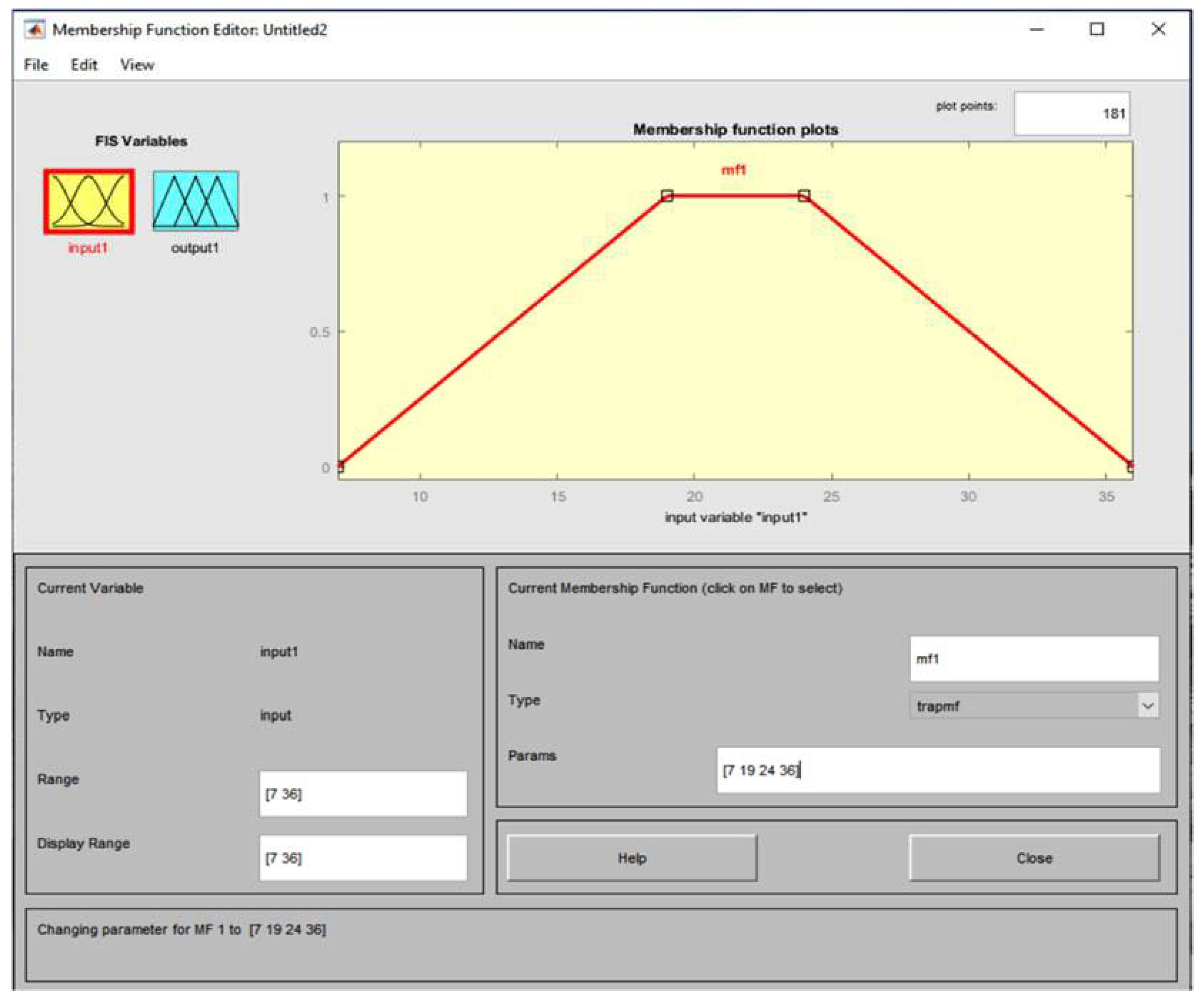
I.: First Case - Isosceles trapezium (trapezium membership function)

In the first case, authors use graphs in the form of an isosceles trapezium in a rectangular system of axes with abscissa temperatures or humidities and ordinates the corresponding fuzzy numbers [0,1]. The vertices of the isosceles trapezoids for temperatures are [7,19,24,36] with graph ordinates [0,1]. While for humidities they have abscissas [0.29, 0.59, 0.64, 0.94] with graph ordinates [0,1].

Specifically, authors type the fuzzy command to open the membership function environment. The following command 3 outputs the degrees of membership by fuzzing the temperature values ranging from [7,36] based on the vertices of the isosceles trapezium [7,19,24,36] (see Figure 1).

ISOSCELESTRAPEZIUMtemperature = trapmf (temperature, [7 19 24 36]) (Command 3)

Therefore, temperature values greater than 7 and close to this value will have a membership degree of approximately 0.1, 0.2, temperature values of 18 and 25 a membership degree of approximately 0.9, temperature values from 19 to 24 a membership degree of 1, and finally temperature values less than value 36 and close to this value will have a membership degree of about 0.1, 0.2. Temperature values 7 and 36 have a membership degree of 0.

The command 4 below outputs the membership degrees by fuzzing the humidity values ranging from [0.29, 0.94] based on the vertices of the isosceles trapezium [0.29, 0.59, 0.64, 0.94] (see Figure 2).

ISOSCELESTRAPEZIUMhumidity = trapmf(humidity, [0.29 0.59 0.64 0.94]) (Command 4)

Therefore, humidity values greater than 0.29 (29%) and close to this value will have a membership degree of about 0.1, 0.2, humidity values of 0.57, 0.58 and 0.65, 0.66 a membership degree of about 0.9, temperature values from 0.59 to 0.64 a membership degree of 1, and finally humidity values smaller than the value 0.94 and close to this value will have a degree of membership of approximately 0.1, 0.2. Humidity values of 0.29 and 0.94 have a membership degree of 0.

II.: Second Case - Random trapezium (trapezoidal membership function)

In the 2nd case authors construct a random trapezium graph in a rectangular system of axes with abscissas of temperature peaks [7,22,23,36] while ordinates the fuzzy corresponding numbers [0,1] and for humidity [0.29, 0.60, 0.61, 0.94] by placing the large base on the abscissa axis.

Command 5 outputs the membership degrees by fuzzing the temperature values based on the vertices of the random trapezium [7,22,23,36] (see Figure 3).

Command 6 outputs the membership degrees by fuzzing the humidity values based on the vertices of the random trapezium [0.29, 0.60, 0.61, 0.94] (see Figure 4).

RANDOMTRAPEZIUMtemperature = trapmf (thermokrasia, [7 22 23 36]) (Command 5)

RANDOMTRAPEZIUMhumidity = trapmf (humidity, [0.29 0.60 0.61 0.94]) (Command 6)

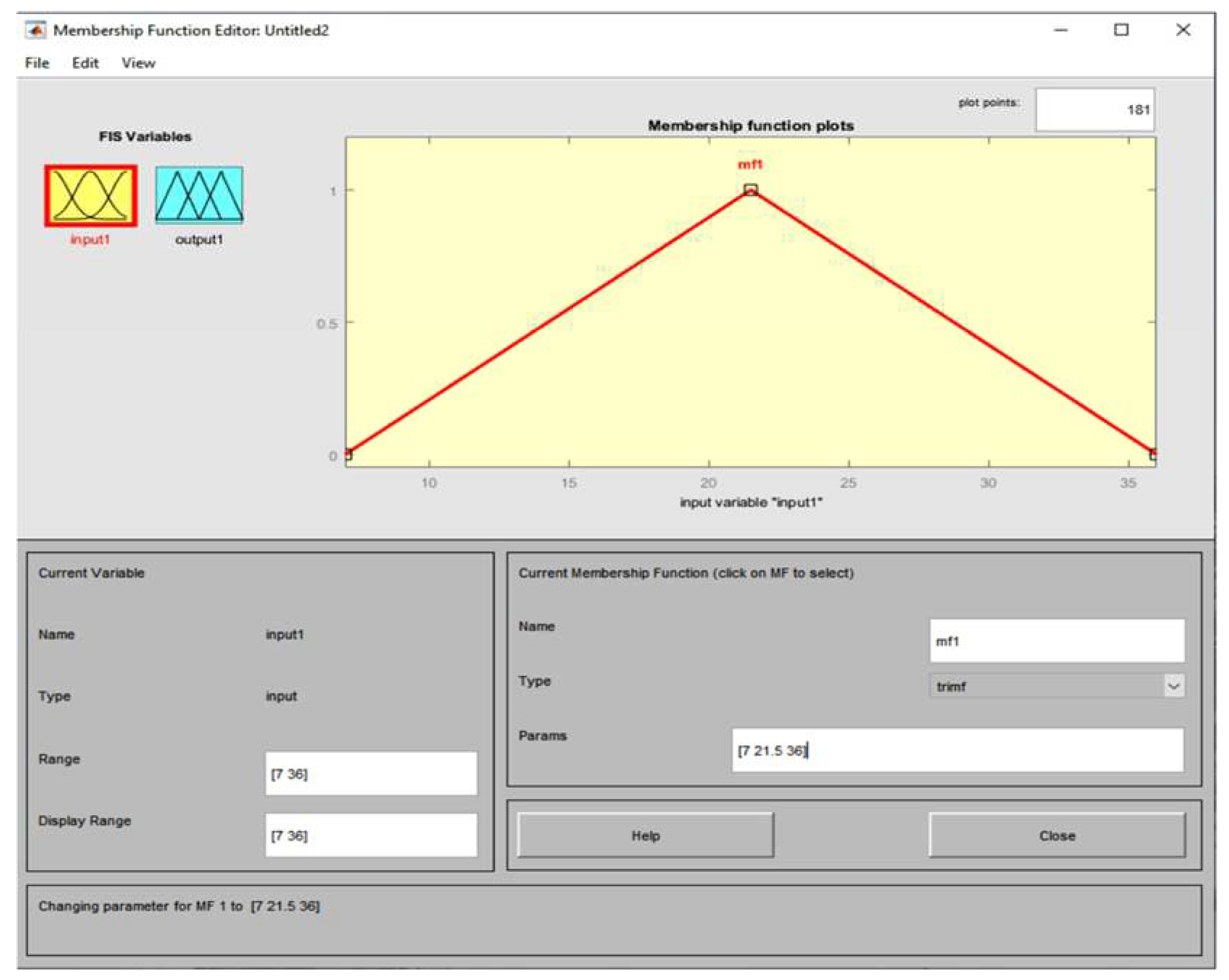
III.: Third Case - Isosceles triangle (triangular membership function)

In the 3rd case we construct an isosceles triangle graph with abscissas of vertices [7, 21.5, 36] having the base on the axis of the abscissas and ordinate of the vertex of the isosceles equal to 1. Similar for isosceles triangle humidities with vertices having abscissa [0.29,0,615,0.94] with maximum ordinate 1 and base on abscissa axis.

Command 7 outputs the membership degrees by fuzzing the temperature values based on the vertices of the isosceles triangle [7, 21.5, 36] (see Figure 5).

Command 8 outputs the membership degrees by fuzzing the humidity values based on the vertices of the isosceles triangle [0.29, 0,615, 0.94] (see Figure 6).

ISOSCELESTRIANGLEtemperature=trimf (temperature, [7, 21.5, 36]) (Command 7)

ISOSCELESTRIANGLEhumidity=trimf (humidity, [0.29 0.615 0.94]) (Command 8)

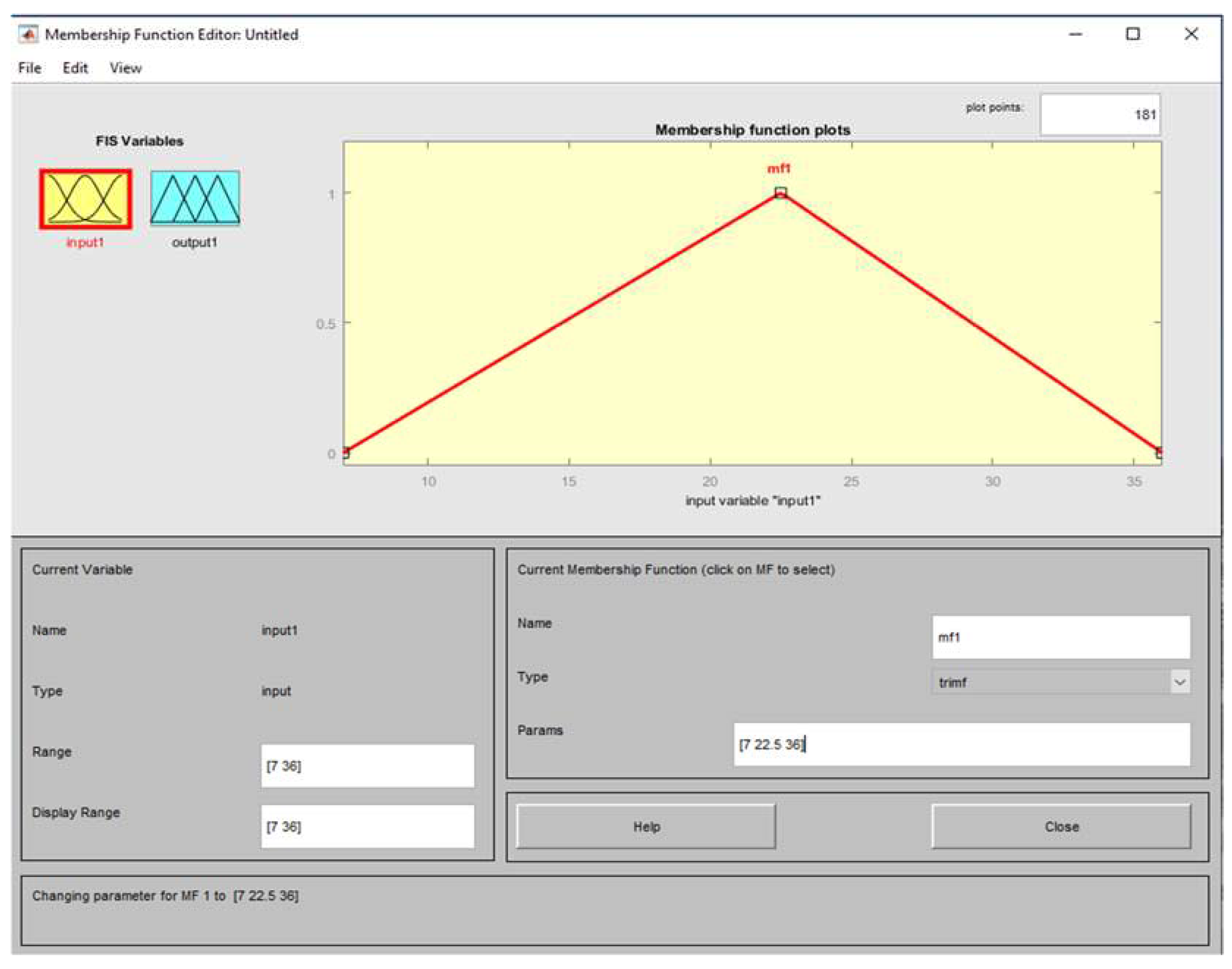
IV.: Fourth Case - Scalene triangle (triangular membership function)

Finally in the 4th case I construct a scalene triangle graph with vertex abscissas [7,22.5,36] temperature graph and [0.29,0.605,0.94] for the humidity graph having ordinate values from [0,1].

Command 9 outputs membership degrees by fuzzing the temperature values based on the vertices of the scalene triangle [7, 22.5, 36] (see Figure 7).

Command 10 outputs membership degrees by fuzzing humidity values based on the vertices of the scalene triangle [0.29, 0,605, 0.94] (see Figure 8).

SCALENETRIANGLEtemperature=trimf(temperature,[7 22.5 36]) (Command 9)

SCALENETRIANGLEhumidity=trimf(humidity,[0.29,0.605,0.94]) (Command 10)

3. Results

Based on the steps in the previous section, we can make the following observations.

For the cases where the degree of membership of temperature = 0, y=0 and the results of the implications remain stable for each m value. Even for the temperatures values of 20°C-24°C with a small deviation we have an almost optimal estimate (the membership degree of temperature is near or equal to 1), while for the values above 24°C the estimates are different with small deviations.

Firstly authors observe that in the isosceles trapezium (first model) the new fuzzy implication takes the value greater or equal to 0.9 with 19 repetitions of the value of m. Also researchers find out that in the isosceles trapezium the new fuzzy implication takes the value equal to 1 with 239 repetitions of the value of m (see Table 1).

Moreover authors observe that in the isosceles triangle (third model) the new fuzzy implication takes the value over to 0.9 with 22 repetitions of the value of m. In this model we find out that in the isosceles triangle the new fuzzy implication takes the value equal to 1 with 289 repetitions of the value of m (see Table 2).

In the first model in a value of m needs fewer repetitions so as to the new fuzzy implication takes the value greater or equal to 0.9 or optimal value equal to 1 in contrast with third model which needs in the value of m needs more repetitions.

In the above Table 3 it is clearly visible that in the case I of the isosceles trapezium in the 19th repetition 74 temperature-humidity pairs of the results of the corollaries in the total of 122 values received the value 1.

In the above Table 4 it is clearly visible that in the case II of the random trapezium in the 20th repetition only 60 temperature-humidity pairs of the results of the corollaries in the total of 122 values received the value 1.

In the above Table 5 it is clearly visible that in the case III of the isosceles triangle in the 22th repetition 66 temperature-humidity pairs of the results of the corollaries in the total of 122 values received the value 1.

In the above Table 6 it is clearly visible that in the case IV of the scalene triangle in the 22th repetition only 60 temperature-humidity pairs of the results of the corollaries in the total of 122 values received the value 1.

At the random trapezium, isosceles and scalene triangle fewer pairs of temperature and humidity values received the value 1 with a worse result giving both the random trapezium (with 20 repetitions) and the scalene triangle (with 21 repetitions) (see Table 4, Table 5 and Table 6). Also the random trapezium and scalene triangle gave the most pairs (61) of temperature–humidity results implication in the total of 122 values that received a value over to 0.9 but not the value equal to 1 (see Table 4 and Table 6).

It therefore follows that the isosceles trapezium gave the best results (more pairs of temperature and humidity values that received the value equal to 1) in relation to the other cases and in shorter times (in a shorter repetitions, 19 repetitions).

Moreover, the isosceles trapezium compared to the rest of the models brought the desired optimal values in faster time repetitions and specifically the 120 temperature-humidity pairs of the results of the implications received the value 1 in the 239th repetition (out of the total of 122 values) (see Table 3). The other models needed more repetitions to achieve the same result (120 pairs of temperature and humidity values), with the third model (case III) needing the most (289) repetitions.

Only one pair of temperature and humidity values (from the total 122 pairs) failed to receive value greater or equal than 0,9 at all four membership degree functions.

4. Discussion

In this paper, authors proposed a new type of fuzzy implication using axioms and theorems of fuzzy logic, which proved to be very reliable and useful for the science of mathematics and Soft Computing. Secondly, authors fuzzified 122 temperature and humidity values using four membership degree functions so as to find the degree of membership of the 122 values for each membership degree function. In third stage the membership degrees of temperature and humidity values applied on the new type of fuzzy implication (16). In this formula variable x represents the degree of membership of humidity values and variable y represents the degree of membership of temperature values. After that, authors made extensive tests in each membership degree function so as to find that value of m that the above formula will get the value greater or equal to 0,9 and the optimal value equal to 1.

Aim of this procedure was to find the precise number of repetitions needed so as to the new fuzzy implication takes the value over to 0.9 and the value equal to 1 or differently in how repetitions the value of m will get that value so that the fuzzy implication takes the optimal value 1 or the value greater or equal to 0.9 in each case (isosceles trapezium, random trapezium, isosceles triangle, scalene triangle).

Moreover, the significance, evaluation and usefulness of this methodology was to find in each membership degree function (from the calculated value of the m or the calculated number of repetitions from the previous step) the number of temperature and humidity pairs where the fuzzy implication takes the optimal value 1 or the value greater or equal to 0.9.

The proposed methodology gives us a way to determine the most suitable fuzzy implication, according to the value of m and according to the data available. So we can specify both the implication formula and also its application mode.

Some of the most important results of the paper that have value are the following:

Authors find that the triangles graphs are a better fit because they don’t have many temperature and humidity values that correspond to the fuzzy number 1 in contrast with the trapezoidal graphs where they have many temperature and humidity values that correspond to the fuzzy number 1. The polygonal graphs for all cases (triangular and trapezoidal) are convex, consequently does not present significant variations in the values of the estimates.

In all membership degree functions after a small number of repetitions which is equal with the value of m, the new type of fuzzy implication (16) takes the value over to 0.9. On the contrary, in all membership degree functions after a large number of repetitions the new type of fuzzy implication (16) takes the value equal to 1. In the isosceles trapezium the fuzzy implication takes the optimal value with fewer repetitions m while in the isosceles triangle needs more repetitions m.

The both trapezoidal membership functions gave better results than the two triangular membership functions. The isosceles trapezium gave the best results (the fewer repetitions and the smallest value of m) while the isosceles triangle gave the worst results (most repetitions and higher values of m).

Also the isosceles trapezium gave the best results (more pairs (74) of temperature and humidity values that received the value equal to 1) in relation to the other three membership degree functions and smaller number of repetitions (19 repetitions). Moreover, the isosceles trapezium compared to the rest of the three membership degree functions brought the desired optimal values in faster time repetitions and specifically the 120 pairs of temperature and humidity values received the value 1 in the 239th repetition. To sum up, in all extensive testing the isosceles trapezium is the most reliable choice for the application of the new type of fuzzy implication.

5. Conclusions and Future Work

In this paper authors have created a model which derives a new type of fuzzy implication based on the operation of t-conorm. The new type is generated by some basic criteria which have been detailed in this paper. During the application process of the methodology, the temperature values were used with the corresponding humidity values, which were clarified using empirically and experimentally four different membership degree functions. After extensive testing we concluded that the new type of fuzzy implication can be effectively applied for values over to 0.9, as it produced very good results in a small number of iterations. Finally from the extracted results, researchers consider that the isosceles trapezium gives the best results of fuzzy implication with respect to the other three membership degree functions used. In particular the isosceles trapezium gave good results both for the value of m=19 and m=239.

As future work, authors propose another new type of fuzzy implication using other axioms and theorems of fuzzy logic, other t-conorm and negations, or fuzzy logic combined with other methods and techniques of Soft Computing (ANFIS). Also, authors can expand the application of the proposed fuzzy implication to other problems, for example geological problems using data from earthquakes such as the intensity and focal depth or the distance or time interval from one earthquake to another. Finally, the new fuzzy implication can find applications in engineering, architecture, environment, mathematics, computing and any science that uses many variables to solve complex problems and deals with decision-making problems.

Author Contributions

Conceptualization, A.K. and B.P.; methodology, A.D., G.S. and A.K.; software, A.D.; validation, A.K. and B.P.; formal analysis, A.D. and A.K, ; investigation, A.D., G.S. and A.K.; resources, A.D. and G.S.; data curation, A.D.; writing—original draft preparation, A.D.; writing—review and editing, A.D. and A.K.; visualization, A.D.; supervision, A.K.; project administration, A.K. and B.P.; All authors have read and agreed to the published version of the manuscript.

Funding

This research received no external funding.

Data Availability Statement

Data supporting reported results are available in a publicly accessible repository that does not issue DOIs and they can be found to the above link: https://freemeteo.gr/mobile/kairos/kavala/istoriko/imerisio-istoriko/?gid=735861&station=5222&date=2021-08-01&language=greek&country=greece&fbclid=IwAR3Ph3AbGLWjGn39AWnLMqarYsgjypBRAtAG9gtcEITSWAVkDwEz4Hffn7M (Retrieved: 4/5/2023)

Acknowledgments

The authors are very thankful to the Editor and referees for their valuable comments and suggestions for improving the paper.

Conflicts of Interest

The authors declare no conflict of interest.

References

Ruan, D.; Kerre, E.E. Fuzzy implication operators and generalized fuzzy method of cases. Fuzzy Sets and Systems 1993, 54, 1, 23–37. ISSN 01650114. [CrossRef]
Makariadis, S.; Souliotis, G.; Papadopoulos, B. Parametric fuzzy implications produced via fuzzy negations with a case study in environmental variables. Symmetry 2021, 13, 3, 509–529. MDPI AG. [CrossRef]
Pagouropoulos, P.; Tzimopoulos, C.D.; Papadopoulos, B.K. A method for the detection of the most suitable fuzzy implication for data applications. In Communications in Computer and Information Science, Proceedings of the 18th International Conference on Engineering Applications of Neural Networks (EANN), Athens, Greece, 25-27 August 2017; Iliadis L., Likas A., Jayne C., Boracchi G. Eds.; Springer Verlag: Volume 744, pp. 242-255. ISBN 978-331965171-2. ISSN 18650929. [CrossRef]
Pagouropoulos, P.; Tzimopoulos, C.D.; Papadopoulos, B.K. A method for the detection of the most suitable fuzzy implication for data applications. Evolving Systems 2020, 11, 3, 467-477. Springer. ISSN 18686478. [CrossRef]
Botzoris, G.N.; Papadopoulos, K. Papadopoulos, B.K. A method for the evaluation and selection of an appropriate fuzzy implication by using statistical data. Fuzzy Economic Review 2015, 20, 2, 19-29. Int. Association for Fuzzy-Set Management and Economy. ISSN 11360593. [CrossRef]
Rapti, M.N.; Papadopoulos, B.K. A method of generating fuzzy implications from n increasing functions and n + 1 negations. Mathematics 2020, 8, 6, art. no. 886, 1-15. MDPI AG. ISSN 22277390. [CrossRef]
Bedregal, B.C.; Dimuro, G.P.; Santiago, R.H.N.; Reiser, R.H.S. On interval fuzzy S-implications. Information Sciences 2010, 180, 8, 1373-1389. ISSN 00200255. [CrossRef]
Balasubramaniam, J. Contrapositive symmetrisation of fuzzy implications-Revisited. Fuzzy Sets and Systems 2006, 157, 17, 2291 – 2310, Elsevier. ISSN 01650114. [CrossRef]
Jayaram, B.; Mesiar, R. On special fuzzy implications. Fuzzy Sets and Systems 2009, 160, 14, 2063-2085 Elsevier. [CrossRef]
Wang, Z.; Xu, Z.; Liu, S.; Yao, Z. Direct clustering analysis based on intuitionistic fuzzy implication. Applied Soft Computing Journal 2014, 23, 1–8 Elsevier. ISSN 15684946. [CrossRef]
Shi, Y.; Van Gasse, B.; Ruan, D.; and Kerre, E.E. On Dependencies and Independencies of Fuzzy Implication Axioms. Fuzzy Sets and Systems 2010, 161, 10, 1388-1405. ISSN 01650114. [CrossRef]
Fernandez-Peralta, R.; Massanet, S.; Mesiarová-Zemánková, A.; Mir, A. A general framework for the characterization of (S, N)-implications with a non-continuous negation based on completions of t-conorms. Fuzzy Sets and Systems 2022, 441, 1–32, Elsevier. ISSN 01650114. [CrossRef]
Fernández-Sánchez, J.; Kolesárová, A.; Mesiar, R., Quesada-Molina, J.J.; Úbeda-Flores, M. A generalization of a copula-based construction of fuzzy implications. Fuzzy Sets and Systems 2023, 456, 197-207, Elsevier. ISSN 01650114. [CrossRef]
Madrid, N.; Cornelis, C. Kitainik axioms do not characterize the class of inclusion measures based on contrapositive fuzzy implications. Fuzzy Sets and Systems 2023, 456, 208–214, Elsevier. ISSN 01650114. [CrossRef]
Pinheiro, J.; Santos, H.; Dimuro, G.P.; Bedregal, B.; Santiago, R.H.N.; Fernandez, J.; Bustince, H. On Fuzzy Implications Derived from General Overlap Functions and Their Relation to Other Classes. Axloms 2023, 12, 1, art. no. 17, pp: 1-24, MDPI. ISSN 20751680. [CrossRef]
Zhao, B.; Lu, J. On the distributivity for the ordinal sums of implications over t-norms and t-conorms. International Journal of Approximate Reasoning 2023, 152, 284-296, Elsevier. ISSN 0888613X. [CrossRef]
Massanet, S.; Mir, A.; Riera, J.V.; Ruiz-Aguilera, R. Fuzzy implication functions with a specific expression: The polynomial case. Fuzzy Sets and Systems 2022, 451, 176–195, Elsevier. ISSN 01650114. [CrossRef]
Souliotis, G.; Papadopoulos, B. Fuzzy Implications Generating from Fuzzy Negations. In Lecture Notes in Computer Science (including subseries Lecture Notes in Artificial Intelligence and Lecture Notes in Bioinformatics), Proceedings of 27th International Conference on Artificial Neural Networks (ICANN 2018), Part 1, Artificial Neural Networks and Machine Learning, Rhodes, Greece, 4–7 October 2018; Kurkova V., Hammer B., Manolopoulos Y., Iliadis L., Maglogiannis I. Eds.; Springer-Verlag: Volume 11139 LNCS, p.p. 736-744. ISBN 978-303001417-9. ISSN 03029743. [CrossRef]
Król, A. Generating of fuzzy implications. In 8th Conference of the European Society for Fuzzy Logic and Technology (EUSFLAT 2013) - Advances in Intelligent Systems, Proceedings of the 8th Conference of the European Society for Fuzzy Logic and Technology (EUSFLAT 2013), Milan, Italy, 11-13 September 2013; Pasi, G., Montero, J., Guicci, D. Eds.; Atlantis Press: Volume 32, pp. 758-763. ISBN 978-162993219-4. [CrossRef]
Souliotis, G.; Papadopoulos, B. An algorithm for producing fuzzy negations via conical sections. Algorithms 2019, 12, 5, MDPI AG: art. no. 89. ISSN 19994893. [CrossRef]
Yang, E. Fixpointed Idempotent Uninorm (Based) Logics. Mathematics 2019, 7, 1, MDPI AG : art. no. 107, Publisher: MDPI AG. ISSN 22277390. [CrossRef]
Massanet, S.; Torrens, J.; Shi, Y.; Van Gasse, B.; Kerre, E.E.; Qin, F.; Baczyński, M.; Deschrijver, G.; Bedregal, B.; Beliakov, G.; Bustince, H.; Fernández, J.; Pradera, A.; Reiser, R.; Hliněná, D.; Kalina, M.; Král’, P.; Drewniak, J.; Sobera, J.; Baczyński, M.; Jayaram, B. Advances in Fuzzy Implication Functions, (Book Series: Studies in Fuzziness and soft Computing STUDFUZZ, volume 300 Series editor Kacprzyk J.) 1st ed.; Baczynski, M.; Beliakov, G.; Sola, H.B.; Pradera, A. Eds.; Springer Berlin, Heidelberg Germany, 2013; VII, p. 209, Hardcover ISBN: 978-3-642-35676-6, e-book ISBN: 978-3-642-35677-3, ISSN: 1434-9922, E-ISSN: 1860-0808. [CrossRef]
Baczynski, M.; Jayaram, B. Fuzzy Implications, (Book Series: Studies in Fuzziness and Soft Computing STUDFUZZ volume 231, Series editor Kacprzyk J.), 1st ed.; Springer-Verlag Berlin Heidelberg, Germany, 2008; XVIII, p. 310, Hardcover ISBN: 978-3-540-69080-1, e-book ISBN: 978-3-540-69082-5, ISSN: 1434-9922, E-ISSN: 1860-0808. [CrossRef]
Metcalfe, G.; Montagna, F. Substructural Fuzzy Logics. Journal of Symbolic Logic 2007, 72, 3, 834–864. ISSN 00224812. [CrossRef]
Ruiz-Aguilera, D., Torrens, J. Residual implications and co-implications from idempotent uninorms. Kybernetika, 2004, 40, 1, 21–38. ISSN 0023-5954.
Grammatikopoulos, D.S.; Papadopoulos, B.K. A Method of Generating Fuzzy Implications with Specific Properties. Symmetry 2020,12, 1, MDPI AG: art. no. 155. ISSN 20738994. [CrossRef]
Massanet, S.; Torrens, J. The law of importation versus the exchange principle on fuzzy implications. Fuzzy Sets and Systems 2011, 168, 1, 47-69. ISSN 01650114. [CrossRef]
Mayor, G. “Sugeno’s negations and t-norms”. Mathware and Soft Computing 1994, 1, 1, 93–98. ISSN 1134-5632.
Smets, P.; and Magrez, P. Implications in fuzzy logic. International Journal of Approximate Reasoning 1987 1, 4, 327-347, Elsevier Science Publishing. ISSN 0888613X. [CrossRef]
Cintula, P. Weakly Implicative (Fuzzy) Logics I: Basic properties. Archive for Mathematical Logic 2006, 45, 6, 673-704. [CrossRef]
Klir, G.J.; and Yuan, Bo. Fuzzy Sets and Fuzzy Logic: Theory and Applications, 1st Ed.; Prentice Hall Press, UpperSaddle River, New Jersey, United States, 1995; pp. 5747. ISBN 10 0131011715.
Trillas, E.; Mas, M.; Monserrat, M.; Torrens, J. On the representation of fuzzy rules. International Journal of Approximate Reasoning 2008, 48, 2, 583–597. ISSN 0888613X. [CrossRef]
Botzoris, G.; Papadopoulos, B. Fuzzy Sets: Applications in Design-Management of Engineer Projects, 1st ed.; Sofia : Greece, Xanthi, 2015; p.p. 424, ISBN-13: 9789606706868 (Book in Greek).
Dombi, J.; Jónás, T. On a strong negation-based representation of modalities. Fuzzy Sets and Systems 2021. 407, 142–160. ISSN 0165-0114. [CrossRef]
Asiain, M.J.; Bustince, H.R.; Mesiar, R.; Kolesárová, A.; Takác, Z. Negations with respect to admissible orders in the interval-valued fuzzy set theory. IEEE Transactions on Fuzzy Systems 2018, 26, 2, 556-568. 1; ISSN 10636706. [CrossRef]
Bustince, H.; Burillo, P.; Soria, F. Automorphisms, negations and implication operators. Fuzzy Sets and Systems 2003, 134, 2, 209-229. ISSN 01650114. [CrossRef]
Drygas, P. Some remarks about idempotent uninorms on complete lattice. In Advances in Intelligent Systems and Computing, Proceedings of the 10th Conference of the European Society for Fuzzy Logic and Technology, Warsaw, Poland 11-15 September 2017; In Advances in Fuzzy Logic and Technology 2017, Proceedings of the EUSFLAT 2017 and 16th International Workshop on Intuitionistic Fuzzy Sets and Generalized Nets (IWIFSGN 2017), Warsaw, Poland 13-15 September 2017; Kacprzyk, J., Szmidt, E., Zadrozny, S., Atanassov, K.T, Krawczak, M., Eds.; Springer: Cham, Switzerland, volume 641, p.p. 648-657. ISBN 978-331966829-1. ISSN 21945357. [CrossRef]
Baczynski, M.; Jayaram, B.; Massanet S.; Torrens, J. Fuzzy Implications: Past, Present, and Future. In Springer Handbook of Computational Intelligence Part of the Springer Handbooks book series (SHB), 1st ed.; Kacprzyk, J., Pedrycz, W., Eds.; Springer: Berlin/Heidelberg, Germany, 2015; pp.183-202. ISBNonline: 978-366243505-2, ISBNprint:978-366243504-5. [CrossRef]
https://freemeteo.gr/mobile/kairos/kavala/istoriko/imerisio-istoriko/?gid=735861&station=5222&date=2021-08-01&language=greek&country=greece&fbclid=IwAR3Ph3AbGLWjGn39AWnLMqarYsgjypBRAtAG9gtcEITSWAVkDwEz4Hffn7M Retrieved: 4/5/2023.

Figure 1. The procedure of the fuzzification of the temperature values ranging from [7,36] based on the vertices of the isosceles trapezium [7,19,24,36].

Figure 2. The procedure of the fuzzification of the humidity values ranging from [0.29, 0.94] based on the vertices of the isosceles trapezium [0.29, 0.59, 0.64, 0.94].

Figure 3. The procedure of the fuzzification of the temperature values ranging from [7,36] based on the vertices of the random trapezium [7,22,23,36].

Figure 4. The procedure of the fuzzification of the humidity values ranging from [0.29, 0.94] based on the vertices of the random trapezium [0.29, 0.60, 0.61, 0.94].

Figure 5. The procedure of the fuzzification of the temperature values ranging from [7, 36] based on the vertices of the isosceles triangle [7, 21.5, 36].

Figure 6. The procedure of the fuzzification of the humidity values ranging from [0.29, 0.94] based on the vertices of the isosceles triangle [0.29, 0.615, 0.94].

Figure 7. The procedure of the fuzzification of the temperature values ranging from [7, 36] based on the vertices of the scalene triangle [7,22.5,36]

Figure 8. The procedure of the fuzzification of the humidity values ranging from [0.29, 0.94] based on the vertices of the scalene triangle [0.29, 0,605, 0.94]

Table 1. Values of fuzzy implication (1) for case I and case II.

	Case I¹	Case II²
n(x)Vŷ^m	Case I¹	Case II²
≥0.9	19	20
=1	239	259

¹ Case I: Isosceles trapezium ² Case II: Random trapezium

Table 2. Values of fuzzy implication (1) for case III and case IV.

	Case I³	Case II⁴
n(x)Vŷ^m	Case I³	Case II⁴
≥0.9	22	21
=1	289	269

³ Case III: Isosceles triangle ⁴ Case IV: Scalene triangle

Table 3. The number of temperature-humidity pairs where the new fuzzy implication takes the value ≥0.9 and the optimal value =1 in case I - isosceles trapezium.

	Case I with 19 repetitions	Case I with 239 repetitions
n(x)Vŷ^m	Case I with 19 repetitions	Case I with 239 repetitions
≥0.9	47	1
=1	74	120

Table 4. The number of temperature-humidity pairs where the new fuzzy implication takes the value ≥0.9 and the optimal value =1 in case II - random trapezium.

	Case II with 20 repetitions	Case II with 259 repetitions
n(x)Vŷ^m	Case II with 20 repetitions	Case II with 259 repetitions
≥0.9	61	1
=1	60	120

Table 5. The number of temperature-humidity pairs where the new fuzzy implication takes the value ≥0.9 and the optimal value =1 in case III - isosceles triangle.

	Case III with 22 repetitions	Case III with 289 repetitions
n(x)Vŷ^m	Case III with 22 repetitions	Case III with 289 repetitions
≥0.9	55	1
=1	66	120

Table 6. The number of temperature-humidity pairs where the new fuzzy implication takes the value ≥0.9 and the optimal value =1 in case IV - scalene triangle.

	Case IV with 21 repetitions	Case IV with 269 repetitions
n(x)Vŷ^m	Case IV with 21 repetitions	Case IV with 269 repetitions
≥0.9	61	1
=1	60	120

Disclaimer/Publisher’s Note: The statements, opinions and data contained in all publications are solely those of the individual author(s) and contributor(s) and not of MDPI and/or the editor(s). MDPI and/or the editor(s) disclaim responsibility for any injury to people or property resulting from any ideas, methods, instructions or products referred to in the content.

© 2024 by the authors. Licensee MDPI, Basel, Switzerland. This article is an open access article distributed under the terms and conditions of the Creative Commons Attribution (CC BY) license (https://creativecommons.org/licenses/by/4.0/).

Copyright: This open access article is published under a Creative Commons CC BY 4.0 license, which permit the free download, distribution, and reuse, provided that the author and preprint are cited in any reuse.

MDPI Initiatives

Important Links

Choose an area of interest and we will send you notifications of new preprints at your preferred frequency.

Disclaimer

Generator of Fuzzy Implications

Abstract

1. Introduction

1.1. Literature Review-Related Work

1.2. Paper outline

2. Theory - New Fuzzy Implication Methods

2.1. Theoretical framework of fuzzy implication

2.2. The new proposed family of fuzzy implication

2.3. Description and application of the new proposed family of fuzzy implications

3. Results

4. Discussion

5. Conclusions and Future Work

Author Contributions

Funding

Data Availability Statement

Acknowledgments

Conflicts of Interest

References

MDPI Initiatives

Important Links

Subscribe