Arctic sea ice prediction holds significant importance for facilitating Arctic route planning, optimizing fisheries management, and advancing the field of sea ice dynamics research. While various deep learning models have been developed for sea ice prediction, they predominantly operate at the seasonal or sub-seasonal scale, often focusing on localized areas, and few cater to full-region daily scale prediction. This study introduces the use of spatiotemporal sequence data prediction models, namely, the convolutional LSTM (ConvLSTM) and predictive recurrent neural network (PredRNN), for the prediction of sea ice concentration (SIC). Our analysis reveals that, when solely utilizing SIC historical data as the input, the ConvLSTM model outperforms the PredRNN model in SIC prediction. To enhance the model's capacity to capture spatiotemporal relationships between multiple variables, we expanded the range of input data types to form the ConvLSTM-multi and PredRNN-multi models. Experimental findings demonstrate that the ConvLSTM-multi model excels in assimilating the influence of reanalysis data on sea ice within the sea ice edge region, thus exhibiting superior performance in predicting daily Arctic SIC over the subsequent 10 days. Furthermore, sensitivity tests on various model parameters highlight the substantial impact of sea surface temperature and prediction date on the accuracy of daily sea ice prediction. Additionally, meteorological and oceanographic parameters primarily affect the prediction accuracy of the thin ice region at the edge of the sea ice.

Keywords:

Subject: Environmental and Earth Sciences - Oceanography

1. Introduction

Global warming has accelerated the rate of melting of the Arctic sea ice [1]. During 1970-2010, Arctic sea ice area decreased by an average of 4% per decade [2]. The rate of sea ice area decline increased dramatically into the 21st century [3,4,5]. The extent of the Arctic sea ice reached its smallest value in the recorded history of satellite data in 2012, at about 3.34 million

{km}^{2}

, while the second lowest value occurred in 2020, at about 3.74 million

{km}^{2}

[6]. The reduced extent of the sea ice presents new opportunities for a number of industries, including Arctic shipping, tourism, fisheries, and oil and gas exploration [7]. Predicting seasonal and daily scale changes in Arctic sea ice is of great practical significance for the safe operation of Arctic shipping lanes and the development and utilization of Arctic resources.

Physical interactions between the atmosphere, ocean, and sea ice are the basis for predicting sea ice. Several studies have already been conducted to predict Arctic sea ice on different spatial and temporal scales and to explore the predictability in different seasons. Blanchart et al. [8] used the outputs of the Community Climate System Model, version 3 (CCSM3) to assess the mechanisms of sea ice persistence, and comparisons with actual observations demonstrated that the model can be used for seasonal to annual predictions of sea ice. Krikken et al. [9] used 15 climate models of CMIP5 to analyze the natural variability in Arctic sea ice from an energy balance perspective and found a strong correlation between the energy balance and the reappearance of sea ice anomalies from the sea ice melting season to the growing season. Guemas et al. [10] reviewed potential sources of Arctic sea ice predictability from months to years, including the persistence and advection of sea ice anomalies, interactions with the oceanic atmosphere, and changes in the radiative forcing. Mohammadi et al. [11] determined the potential predictability of Arctic winter sea ice using a sea ice–ocean coupling model, noting high predictability of sea ice concentration (SIC) and sea ice edge position over a 10-day period. Cruz et al.[12] investigated sea-ice predictability from seasonal to annual scales using a variety of climate models, emphasizing the importance of the reoccurring effects of sea ice anomalies, and observed that anomalies in SIC in the Barents Sea are highly negatively correlated with local sea surface temperature anomalies. Onarheim et al.[13] showed that ocean heat transport (OHT) variability plays an important role in winter sea ice variability in the Barents Sea, and that the use of the OHT can lead to predictions two years in advance. These studies provide knowledge on the predictability of sea ice associated with a wide range of physical processes, while emphasizing the importance of selecting predictors that are relevant to the target location and time scale.

The main approaches to Arctic sea ice prediction are numerical simulations, statistical predictions and deep learning. Numerical simulation methods are based on physical links between temperature changes, humidity transport, wind field models, cloud cover and ocean heat fluxes. Major climate simulation centers around the world have released some atmospheric and oceanic simulation data. Their adoption of climate models relies on real-time inputs of observational conditions in the data assimilation process. At the same time, due to the limitations of a single climate model and the large differences in the results of different models, it is necessary to determine the assigned weights of each climate model based on its contribution to the simulation of the current climate mean, and then take a weighted average to improve the accuracy of sea ice prediction. In practice, this treatment does not eliminate the effect of model bias on sea ice prediction. In addition, many processes in the dynamic model of sea ice need parameterization, and the current model lacks modeling of rheology, ice thickness distribution, wave–ice interaction, landing ice, melting water and size distribution of floating ice[14]. Statistical methods are used to predict the state of sea ice according to historical data. With the thinning of sea ice, the average state of sea ice has changed significantly. In addition, most statistical models are linear models, which cannot learn the nonlinear relationship between variables in the Arctic climate system. Because the nonlinear feedback mechanism plays an important role in the coupling system of Arctic atmosphere, ocean and sea ice, it is necessary to predict Arctic sea ice using a nonlinear model. Deep learning technology has a strong nonlinear learning ability. Chi et al. and Choi et al. input the monthly average SIC data of the National Snow and Ice Data Center (NSIDC) into the multilayer perceptron (MLP) and the long and short-term memory (LSTM) models to predict the monthly average of SIC, and found that the results are better than the traditional autoregressive (AR) model[15,16]. Kim et al.[17] used the integrated data of a regional climate model (RCM) as input variables, and used the deep neural network (DNN) method to deal with the nonlinear relationship between SIC and climate variables. As a result, they predicted the SIC in the Kara Sea and Barents Sea in the next 10-20 years. Fritzner et al.[18] compared the prediction accuracy of a high-resolution dynamic assimilation model, K-NN model and FCN model for the next 7 days, and pointed out that the FCN model can provide similar prediction results to the dynamic assimilation model. Kim et al.[19] input eight predictors into the CNN model to predict the monthly average SIC in the next month, and the results were better than that of the RF model. Andersson et al.[20] put forward a model of a probabilistic sea ice prediction system. The model used climate simulation and observation data as the input data to predict the monthly average SIC in the next six months. The results showed that the IceNet model has a high accuracy in predicting the sea ice range, and it is superior to the SEAS5 dynamic model in predicting extreme sea ice events in summer. Liu et al.[21] used the convolutional LSTM (ConvLSTM) model to predict SIC in the Barents Sea over the next six weeks. They added ERA-Interim reanalysis data to the training dataset, and used the covariance between different variables and the spatiotemporal correlation to complete the prediction of regional SIC. The results were better than the linear regression model. At present, the deep learning method is mainly used to predict the sub-seasonal scale of regional sea ice. Because the daily short-term forecast of SIC is very important for maritime shipping decision-making, it is urgent to attain the accurate daily short-term forecast of SIC.

The ConvLSTM and predictive recurrent neural network (PredRNN) models exhibit the capacity to capture spatiotemporal correlations among diverse input parameters, enabling them to theoretically predict spatiotemporal sequence data. This study introduces these models into the realm of the high-precision daily scale short-term prediction of Arctic sea ice. Initially, we compare the predictive performance of the ConvLSTM and PredRNN models when only SIC is utilized as the input. Subsequently, we enhance the input data by incorporating meteorological parameters that influence both SIC and the sea boundary, leading to the formation of ConvLSTM-multi and PredRNN-multi models. Through an investigation of the spatiotemporal correlations between SIC and meteorological parameters, we observe a substantial enhancement in the model's predictive capability for the sea ice edge region. Furthermore, this paper conducts a quantitative analysis to discern the model's sensitivity to the input meteorological parameters, pinpointing the key meteorological variables that affect the prediction accuracy of SIC.

2. Data and methods

2.1. Data

We used SIC data from the NSIDC and reanalysis data from ERA5, provided by the European Centre for Medium-Range Weather Forecasts (ECMWF), as the training set, spanning the period from 1988 to 2021. The NSIDC SIC dataset is derived from observations made by the scanning multichannel microwave radiometer (SMMR) carried by the Nimbus-7 satellite, the special sensor microwave imager (SSM/I) sensors carried by the National Defense Meteorological Satellite Program (DMSP)-F8, -F11 and -F13 satellites and the special sensor microwave imager/sounder (SSMIS) sensors carried by DMSP-F17. Among the NSIDC datasets, we utilized the NASA Bootstrap algorithm-derived dataset for our research. The product is provided in the form of a daily average, with polar stereo projection (45°W, 70°N), spatial resolution of 25km×25km and grid number of 448×304. The values within this dataset range from 0, signifying the absence of ice in the grid, to 100, indicating complete sea ice coverage. The primary sources of error in these data arise from thin ice (ranging from 30% to 50%) and surface melting (ranging from 10% to 30%) [22]. The Arctic Ocean covered by this dataset predominantly encompasses the Sea of Okholtsk, Bering Sea, Chukehi Sea, Beaufort Sea, Canadian Archipelago, Hudson Bay, Baffin Bay, Greenland Sea, Norwegian Sea, Barents Sea, Kara Sea, Laptev Sea, East Siberian Sea and Central Arctic Sea. The distribution of sea areas is illustrated in Figure 1. The NSIDC takes SIC=15% as the sea ice boundary threshold, and the region with SIC≥15% is considered as the sea ice area.

The ERA5 dataset is a global meteorological dataset in which the ECMWF combines meteorological model data with observation data from all over the world, with a spatial resolution of

0.25 ° \times 0.25 °

[23]. Table 1 details the specific parameters within the ERA5 dataset utilized as inputs for our model, include sea surface temperature (SST), 2m temperature (T2M), skin temperature (SKT), surface solar radiation downwards (SSRD), mean sea level pressure (MSL), 10m u-component of wind (U10) and 10m v-component of wind (V10). The hourly value of ERA5 data is converted into a daily average, resampled into a grid consistent with SIC data, and the value is normalized to [0,1].

SIC, ERA5 15 days in advance, land mask, cosine and sine values of dates are fused together to form a series of 10 consecutive days as training samples. The dataset is divided into training dataset (1988-2018), verification dataset (2019) and test dataset (2020-2021). The Arctic sea ice area in September 2020 was the second lowest level in the recorded history of satellite data (greater only than in September 2012)[24], which serves as a fitting evaluation point for assessing the model's predictive performance under extreme conditions. All three datasets were partitioned into 10-day sequences to achieve a random input of 10 days of historical data to predict the SIC for the next 10 days. To analyze to what extent and how the atmospheric conditions and oceanic variables affected the accuracy of the model predictions, the models were trained using the mode of inputting both single and multiple predictors (Table 1).

In addition, the sixth phase of the Coupled Model Intercomparison Project (CMIP6) "selected models" nominated by the Sea-Ice Model Intercomparison Project (SIMIP) community[25] were used. SIMIP aims to compare and evaluate the performance of different sea-ice models, collect different simulation results and establish a standardized database, identify model strengths and weaknesses and uncertainties, improve the accuracy of sea ice models, and lay the foundation for future sea-ice prediction studies. The “selected models” in Table A 1 provide the best estimates of the future evolution of Arctic sea ice, and the daily average SIC provided by three CO2 emission scenarios, SSP126, SSP245, and SSP585, were chosen for comparison with the deep learning model.

2.2. Model

SIC data should be predicted using the spatiotemporal sequence prediction model. The spatiotemporal sequence is a dynamic system in which historical observations with arbitrary length J evolve over time, and observations at each moment can be represented on an M×N grid. Thus, the observation at any time can be represented by a tensor

X \in ℝ^{J \times M \times N}

, where J denotes the domain of the observed features. If we record observations periodically, we will obtain a sequence of tensors, while observations over period of T are denoted as

X_{i n} = \{X_{1}, \dots, X_{T}\}

. The model is designed to predict the sequence

{\hat{X}}_{out} = \{{\hat{X}}_{T + 1}, \dots, {\hat{X}}_{T + K}\}

for the next K time steps, given

X_{i n}

. For the training pairs

{\{(X_{in}^{n}, X_{out}^{n})\}}_{n}

formed by all SIC data, a set of parameters

θ^{'}

is found by using random gradient descent to ensure that the log-likelihood of the generated target sequence

X_{o u t}

is the maximum when the input data

X_{i n}

are provided:

θ' = \underset{θ}{\arg \max} \sum_{(X_{in}^{n}, X_{out}^{n})} \log P (X_{out}^{n} ∣ X_{in}^{n}; θ)

(1)

In this study, we present the ConvLSTM model [26] and PredRNN model [27], which are commonly employed for spatiotemporal sequence data prediction, to realize the prediction of SIC. The ConvLSTM model replaces matrix multiplication with convolution operations within the LSTM gating structure unit. This alteration allows it to simultaneously capture both temporal and spatial features in the data, effectively transforming the traditional encoding–decoding structure into an encoding–forecasting structure. The gating formula for the ConvLSTM unit is:

\begin{matrix} g_{t} = \tanh (W_{x g} * X_{t} + W_{h g} * H_{t - 1} + b_{g}) \\ i_{t} = σ (W_{x i} * X_{t} + W_{h i} * H_{t - 1} + W_{c i} ⊙ C_{t - 1} + b_{i}) \\ f_{t} = σ (W_{x f} * X_{t} + W_{h f} * H_{t - 1} + W_{c f} ⊙ C_{t - 1} + b_{f}) \\ C_{t} = f_{t} ⊙ C_{t - 1} + i_{t} ⊙ g_{t} \\ o_{t} = σ (W_{x o} * X_{t} + W_{h o} * H_{t - 1} + W_{c o} ⊙ C_{t} + b_{o}) \\ H_{t} = o_{t} ⊙ \tanh (C_{t}) \end{matrix}

(2)

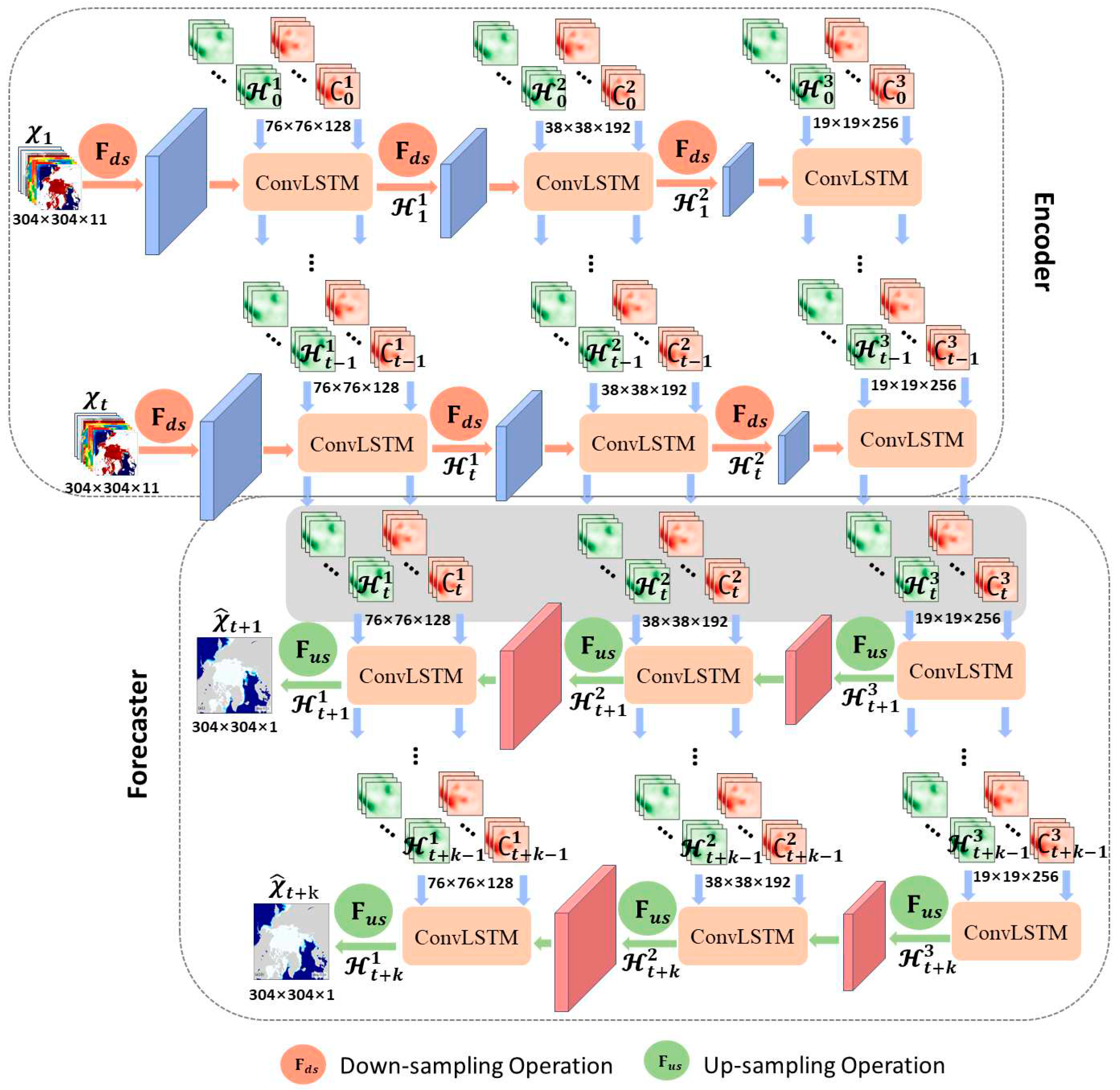
where

i_{t}

is the input gate;

f_{t}

is the forgetting gate;

∁_{t}

is the unit storage state;

o_{t}

is the output gate;

H_{t}

is the hidden state;

W

is the weight matrix, with the subscript describing the correspondence between the weight matrix and the state of each gate;

χ

is the input;

b

is the bias; ∗ is the convolution operation;

⊙

is the Hadamard product;

σ

is the sigmoid activation function;

\tan h

is the hyperbolic tangent activation function; and the subscript

t

denotes the time step. Figure 2 illustrates the ConvLSTM network framework, which consists of a three-layer stack of ConvLSTM units employed in the encoding–forecasting framework. In this framework, the encoder incorporates a down-sampling operation, while the forecaster utilizes an up-sampling operation before each layer of input at each time step. The training data input follows the traditional sequence-to-sequence approach [28]. Historical observations are input into the encoder during the training phase, and the state layers generated at each layer of the encoder (the shaded region in Figure 2) are transmitted to the forecaster. The loss function is determined by comparing predicted values to actual values, and model parameters are adjusted through backpropagation until Equation 1 is satisfied.

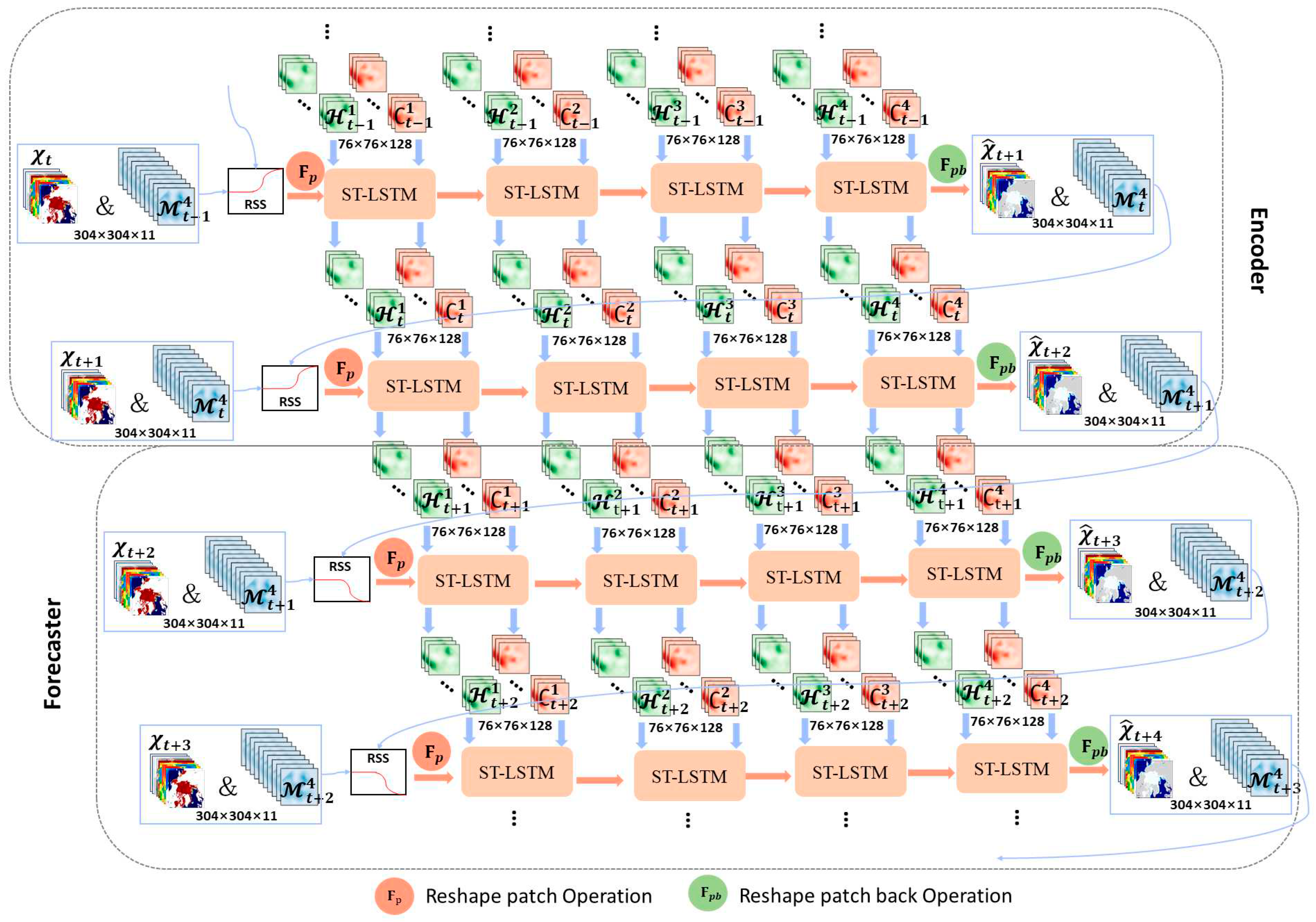
The PredRNN exhibits three distinctions from the ConvLSTM framework: (1) It introduces a spatiotemporal memory-state circulation method, depicted by the blue arrows in Figure 3, which enhances the lower layer's capability to learn top-layer features from the previous time step; (2) The unit responsible for the spatiotemporal memory stream employs a dual-stream memory transition mechanism involving

∁_{t}

and

Μ_{t}

. This results in memory states that cannot be decoupled spontaneously. To address this, a convolutional layer is added to the

∁_{t}

and

Μ_{t}

increments at each time step, and the spatial distances between them are extended using a novel decoupling loss function. This approach trains different memory states to focus on long-term and short-term spatiotemporal changes. (3) The model training approach incorporates the reverse scheduled sampling (RSS) [29] method for data input. This technique forces the model to randomly conceal true observations in the encoder to learn long-term dynamics, with the probability of concealing true observations decreasing with the number of iterations. This ensures that the model has the same likelihood of inputting true observations during both the training and prediction phases. In (1), the network is enabled to learn the complex nonlinear variations in short-term motions. However, the state layer transfer path stretching across time brings the problem of gradient vanishing, making it challenging to capture long-term dependencies. Therefore, a dual-stream memory transition mechanism is introduced to achieve a short-term recursion depth and long-term consistency by combining the original memory unit

∁_{t}

and the new memory unit

Μ_{t}

to form a unit named ST-LSTM, which is calculated as follows:

\begin{array}{l} g_{t} = t a n h (W_{x g} * χ_{t} + W_{h g} * H_{t - 1}^{l} + b_{g}) \\ i_{t} = σ (W_{x i} * χ_{t} + W_{h i} * H_{t - 1}^{l} + b_{i}) \\ f_{t} = σ (W_{x f} * χ_{t} + W_{h f} * H_{t - 1}^{l} + b_{f}) \\ C_{t}^{l} = f_{t} ⊙ C_{t - 1}^{l} + i_{t} ⊙ g_{t} \\ g_{t}^{'} = t a n h (W_{x g}^{'} * χ_{t} + W_{m g} * M_{t}^{l - 1} + b_{g}^{'}) \\ i_{t}^{'} = σ (W_{x i}^{'} * χ_{t} + W_{m i} * M_{t}^{l - 1} + b_{i}^{'}) \\ f_{t}^{'} = σ (W_{x f}^{'} * χ_{t} + W_{m f} * M_{t}^{l - 1} + b_{t}^{'}) \\ M_{t}^{l} = f_{t}^{'} ⊙ M_{t}^{l - 1} + i_{t}^{'} ⊙ g_{t}^{'} \\ o_{t} = σ (W_{x o} * χ_{t} + W_{h o} * H_{t - 1}^{l} + W_{c o} * C_{t}^{l} + W_{m o} * M_{t}^{l} + b_{o}) \\ H_{t}^{l} = o_{t} ⊙ t a n h (W_{1 \times 1} * [C_{t}^{l}, M_{t}^{l}]) \end{array}

(3)

The PredRNN network framework comprises four layers of interconnected ST-LSTM units. As illustrated in Figure 3, the input data undergo reverse scheduled sampling (RSS), progressively increasing the likelihood of true observations being incorporated in the encoder, while inversely decreasing in the forecaster. The state unit

H_{t}^{l}

and memory unit

M_{t}^{l}

circulate along the orange arrows in the diagram. Subsequently, the memory unit

M_{t}^{l}

flows directly along the blue arrows, transitioning from the uppermost layer of the preceding time step to the lower layer of the subsequent time step, thereby establishing the circulation of short-term memory states.

2.3. Evaluation metrics

Mean absolute error (MAE) (Equation 4), root mean square error (RMSE) (Equation 5), normalized root mean square error (nRMSE) (Equation 6), anomalous correlation coefficient (ACC) (Equation 7), Nash–Sutcliffe efficiency (NSE) (Equation 8), and structure similarity index measure (SSIM) (Equation 9) are used to assess the model's performance in predicting SIC. MAE and RMSE are used to measure the absolute difference between the model's predictions and observed values, with lower values indicating superior predictive capability. nRMSE is computed by dividing RMSE by the standard deviation of observed values, thereby offering a more precise depiction of the residuals in the sea-ice edge region within the model's predictions. It is expressed as a percentage, with lower values signifying reduced residuals. ACC serves as an indicator of the fidelity of predicted anomalies and the degree to which predicted values align with the actual data, producing values within the range of +1 to -1. A value closer to +1 denotes greater consistency between predicted and observed values. NSE is employed to gauge the precision of the model's output values within the range of

- \infty

to 1. Values approaching 1 signify a more accurate model. SSIM quantifies the structural resemblance between predicted and observed values, with values approaching 1 indicating a higher structural similarity.

M A E = \frac{|X_{o b s, i} - X_{m o d e l, i}|}{n}

(4)

R M S E = \sqrt{\frac{\sum_{i = 1}^{n} {(X_{o b s ​, i} - X_{m o d e l, i})}^{2}}{n}}

(5)

n R M S E = \sqrt{\frac{\sum_{i = 1}^{n} {(X_{o b s ​, i} - X_{m o d e l, i})}^{2}}{\sum_{i = 1}^{n} {(X_{o b s ​, i} - \bar{X_{o b s}})}^{2}}}

(6)

A C C = \frac{\sum_{i = 1}^{n} (X_{m o d e l, i} - \bar{X_{m o d e l}}) (X_{o b s, i} - \bar{X_{o b s}})}{\sqrt{{\sum_{i = 1}^{n} (X_{m o d e l, i} - \bar{X_{m o d e l}})}^{2} {\sum_{i = 1}^{n} (X_{o b s, i} - \bar{X_{o b s}})}^{2}}}

(7)

N S E = 1 - \frac{\sum_{i = 1}^{n} {(X_{o b s, i} - X_{m o d e l, i})}^{2}}{\sum_{i = 1}^{n} {(X_{o b s, i} - \bar{X_{o b s}})}^{2}}

(8)

S S I M (o b s, m o d e l) = \frac{(2 μ_{o b s} μ_{m o d e l} + C_{1}) (2 σ_{o b s m o d e l} + C_{2})}{(μ_{o b s}^{2} + μ_{m o d e l}^{2} + C_{1}) (σ_{o b s}^{2} + σ_{m o d e l}^{2} + C_{2})}

(9)

Model prediction errors primarily manifest at the sea ice edge, an area of significance for Arctic shipping and navigation. Therefore, it is imperative to validate the prediction accuracy of the sea-ice edge position. Melsom et al. [30] proposed employing three metrics, namely, the mean ice edge displacement (

D_{AVG}^{IE}

), the integrated ice edge error (IIEE) average displacement (

D_{AVG}^{IIEE}

), and the IIEE bias (

Δ^{IIEE}

), to assess the accuracy of the model's sea-ice edge prediction.

D_{AVG}^{IE}

measures the shortest Euclidean distance between the actual observed sea-ice edge grid cell points and the model's sea-ice edge grid cell points (Equation 10). Here,

N_{o}

N_{m}

denote the number of grids for observed and predicted values, while

d_{o}^{n}

d_{m}^{n}

represent the distance displacements between the observed and predicted values corresponding to the nth grid of the edge.

D_{AVG}^{IIEE}

defines the integral displacement between the observed and predicted ice edges (Equations 11-12). Error estimation by integration reduces the effect of small-sized localized ice features (e.g., polygonal openings) on the total displacement[31].

Δ^{IIEE}

quantifies the disparity between observed and predicted ice (Equation 13), with a positive deviation indicating that the predicted ice exceeds the observed value, and vice versa.

In these equations,

c_{m}, c_{o}

and

c_{e}

represent the predicted values at grid points, the observed values at grid points, and the constant values defining the sea ice boundaries, respectively.

L_{O}

L_{M}

are the observed and predicted ice edge lengths.

A^{I I E E}

encompasses the total number of grid cells in the over-predicted and under-predicted ice regions, with

α^{I I E E}

representing the difference between them.

γ_{A V G}

determines the robustness of sea-ice edge error measurement results, with larger values indicating greater sensitivity to the formulation of the sea-ice edge displacement error (Equation 14).

D_{AVG}^{IE} = \frac{1}{2} [\frac{1}{N_{O}} \sum_{n = 1}^{N_{O}} d_{o}^{n} + \frac{1}{N_{M}} \sum_{n = 1}^{N_{M}} d_{m}^{n}]

(10)

\begin{array}{l} A^{IIEE} = A^{+} + A^{-}, A^{+} = \sum_{A} a^{+}, a^{+} = \{\begin{cases} a, c_{m} > c_{e} \land c_{o} < c_{e} \\ 0 \end{cases} \\ α^{IIEE} = A^{+} - A^{-}, A^{-} = \sum_{A} a^{-}, a^{-} = \{\begin{cases} a, c_{o} > c_{e} \land c_{m} < c_{e} \\ 0 \end{cases} \end{array}

(11)

D_{AVG}^{IIEE} = \frac{2}{L_{O} + L_{M}} A^{IIEE}

(12)

Δ^{IIEE} = \frac{2}{L_{O} + L_{M}} α^{IIEE}

(13)

r_{AVG} = \frac{D_{AVG}^{IE}}{D_{AVG}^{IIEE}}

(14)

3. Results and discussion

3.1. Daily scale predictions of sea ice concentration

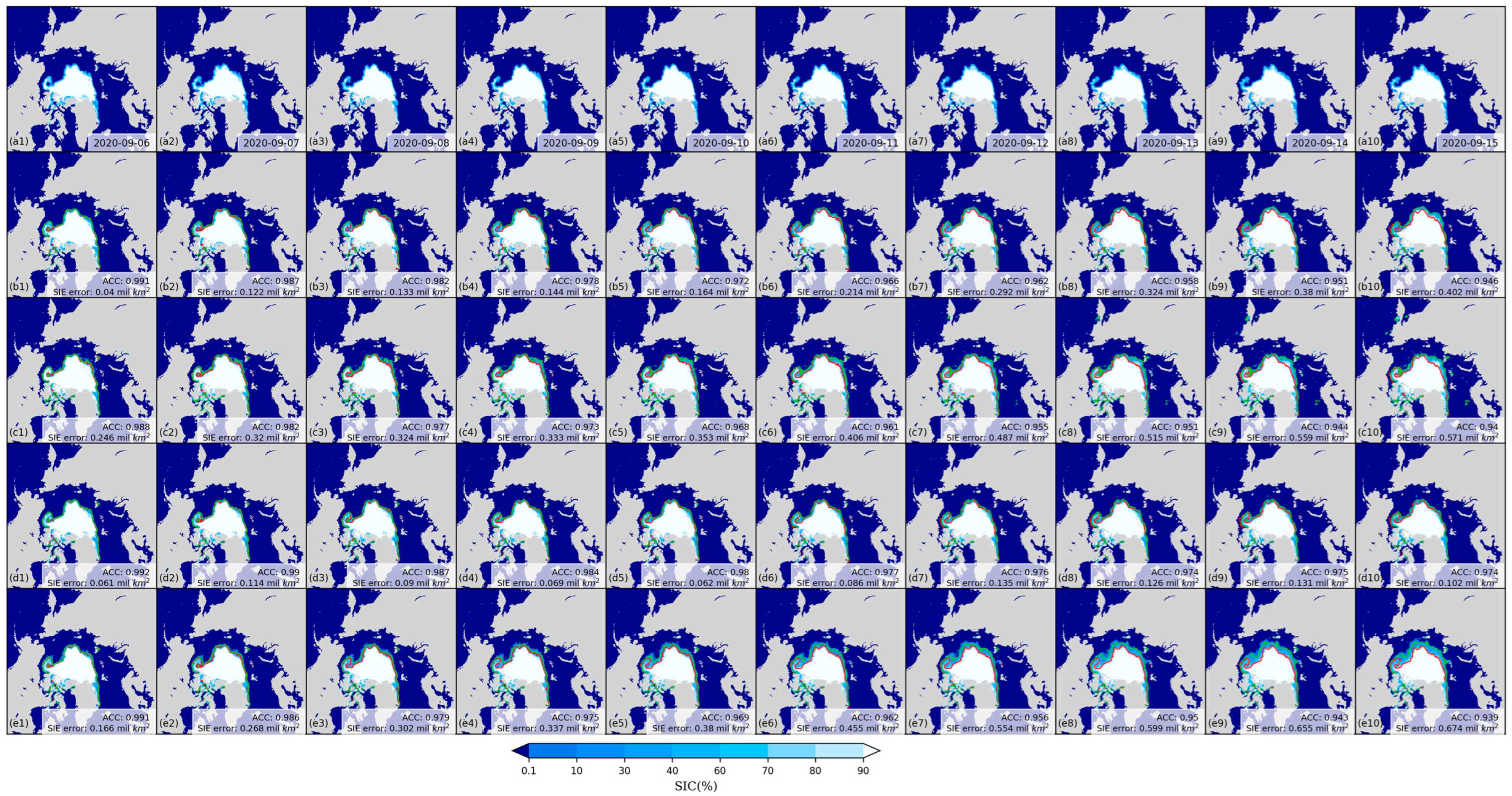
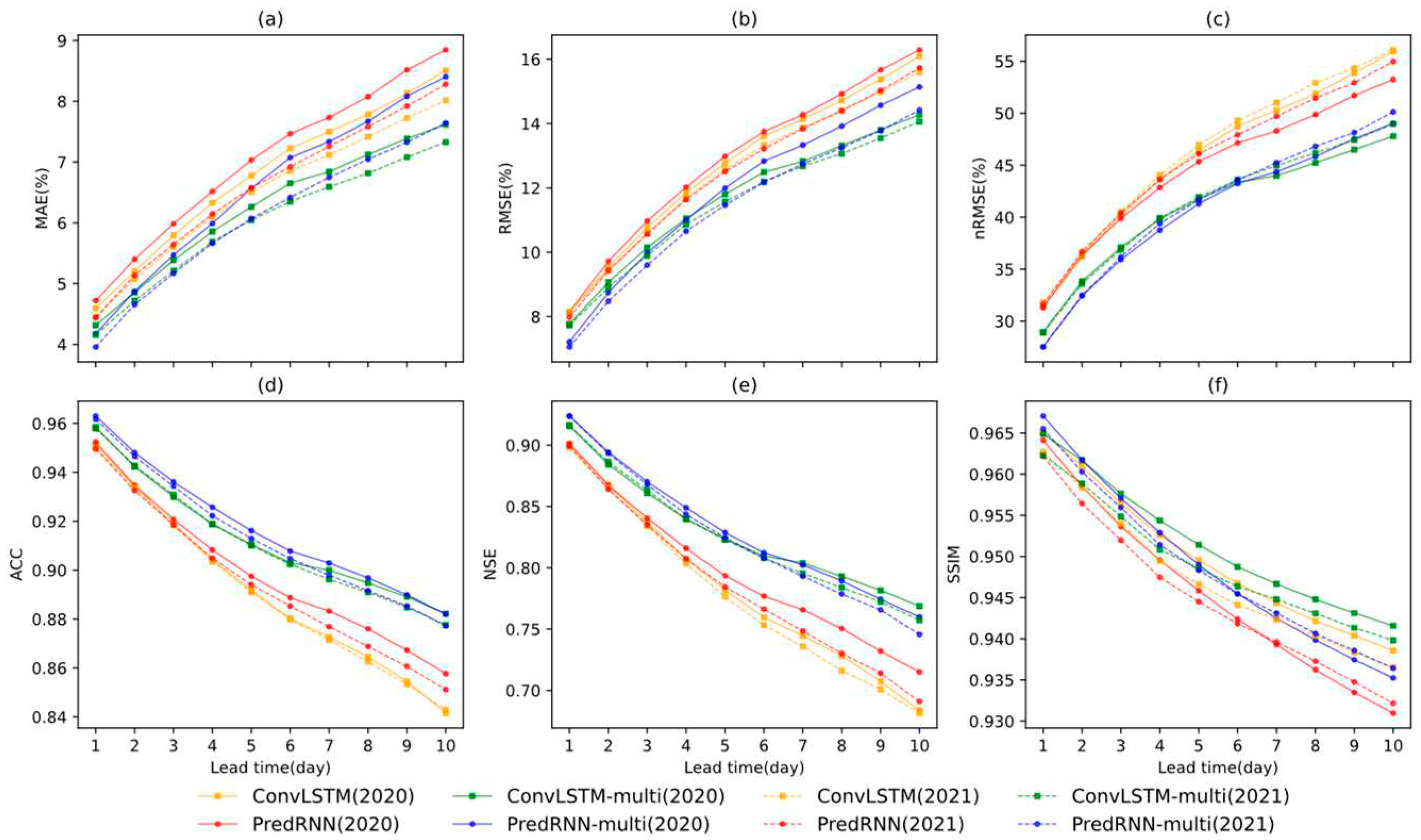
Figure 4 depicts the distribution of average prediction accuracy metrics (MAE, RMSE, nRMSE, ACC, NSE, and SSIM) values for the ConvLSTM, PredRNN, ConvLSTM-multi, and PredRNN-multi models for the years 2020 and 2021. As shown in Figures 4a and 4b, the daily average prediction accuracy of SIC in 2020 and 2021 follows the order of ConvLSTM-multi, PredRNN-multi, ConvLSTM, and PredRNN, from high to low, for MAE and RMSE. The metrics nRMSE, ACC, and NSE exhibit sensitivity to the prediction accuracy of the sea ice edge region. As evidenced by Figure 4c, d, and e, the prediction accuracy of the multi-predictor models ConvLSTM-multi and PredRNN-multi in the thin ice region significantly outperforms that of the single predictor models. PredRNN-multi demonstrates superior prediction accuracy in the initial six days, but it is subsequently surpassed by ConvLSTM-multi. Figure 4f illustrates that the ConvLSTM model outperforms the PredRNN model in terms of the SSIM between predicted values and observed values. Notably, the ConvLSTM-multi model excels, capturing the shape changes in Arctic sea ice coverage for 2020 and 2021. Figure A 2 shows the SIC distribution of observed and predicted values from September 6 to September 15, 2020, for ConvLSTM, PredRNN, ConvLSTM-multi, and PredRNN-multi models. It is evident that the sea ice edge's shape in the ConvLSTM-multi model aligns most closely with the observed values.

Overall, the prediction accuracy of the four models significantly surpasses the average prediction accuracy of the CMIP6 model in three prospective climate scenarios (Table 2). On the 10th day, the prediction accuracy of the four models reaches its weakest values (MAE: 8.45%, RMSE: 15.96%, nRMSE: 48%, ACC: 0.88, NSE: 0.76), which is superior to the ensemble prediction accuracy of the best model (SSP126 in 2020: MAE: 19.67%, RMSE: 29.13%, nRMSE: 69%, ACC: 0.76, NSE: 0.53).

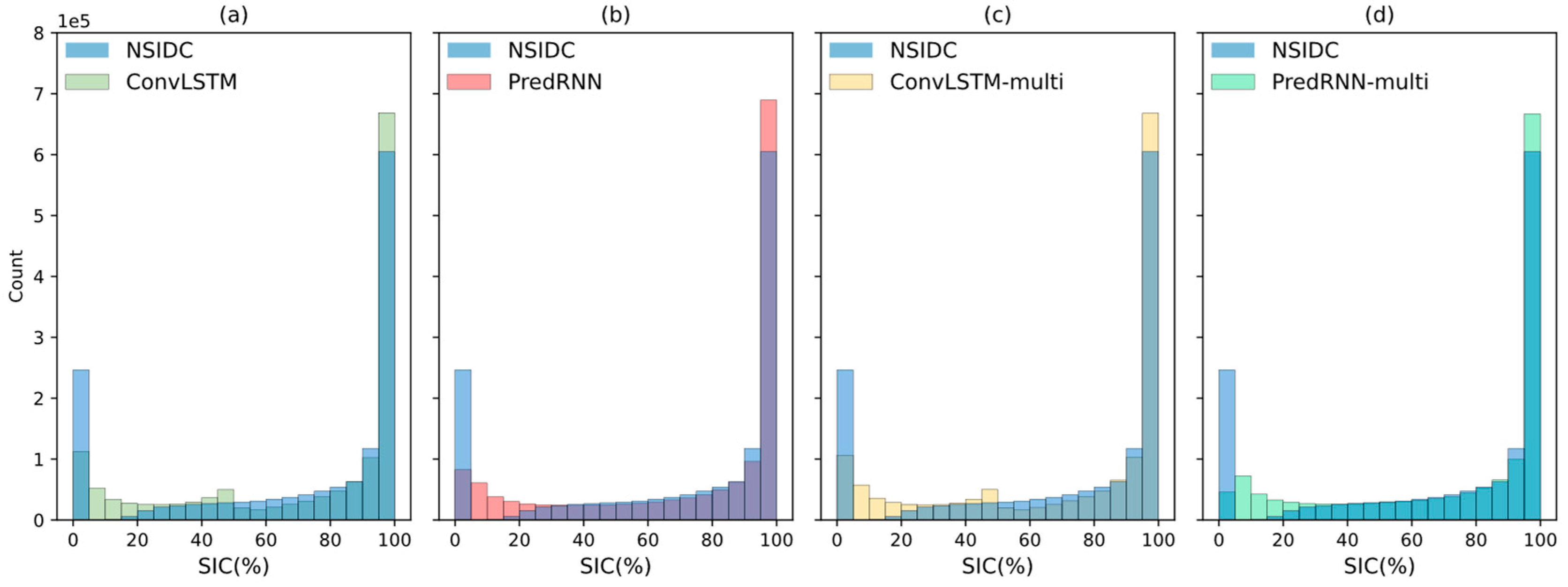
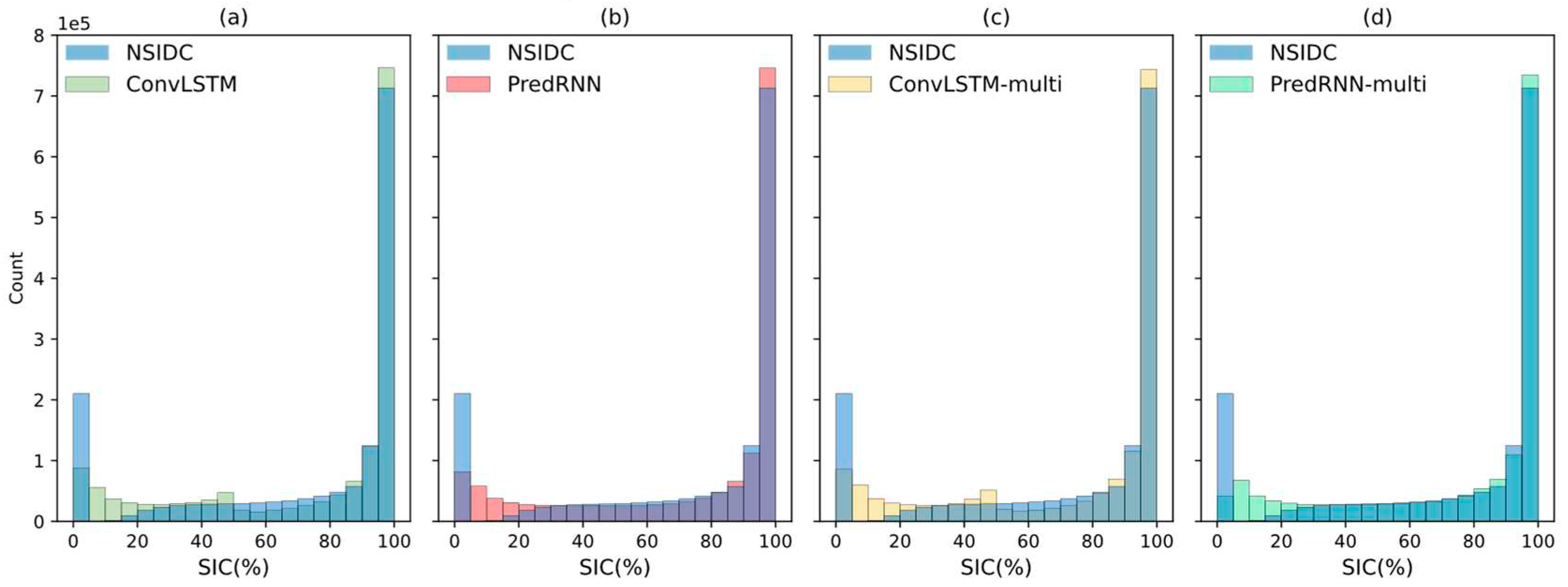
Figure 5 and Figure 6 display comparative histograms illustrating the distribution of SIC intervals, observed from NSIDC data, and those predicted by four distinct models during the melting season spanning from June to September in the years 2020 and 2021. Since NSIDC assigns all regions with less than 15% SIC to 0, the number of grids with 0 in the predicted SIC values of the four models is obviously less than that of NSIDC SIC. The comparison results show that the number of grids predicted by ConvLSTM and ConvLSTM-multi models is high in 40%~50% and low in 50%~80%. The predicted values of PredRNN and PredRNN-multi models exhibit a remarkable level of agreement with NSIDC SIC in 30%~90%; The predicted values of the four models are low in 90%~95% and high in 95%~100%. The difference between the predicted grid number and the observed grid number of the PredRNN-multi model in 80%~100% is smaller than that of the PredRNN model. The interval distribution of SIC predicted by the PredRNN-multi model is most consistent with the distribution of NSIDC SIC in the melting season.

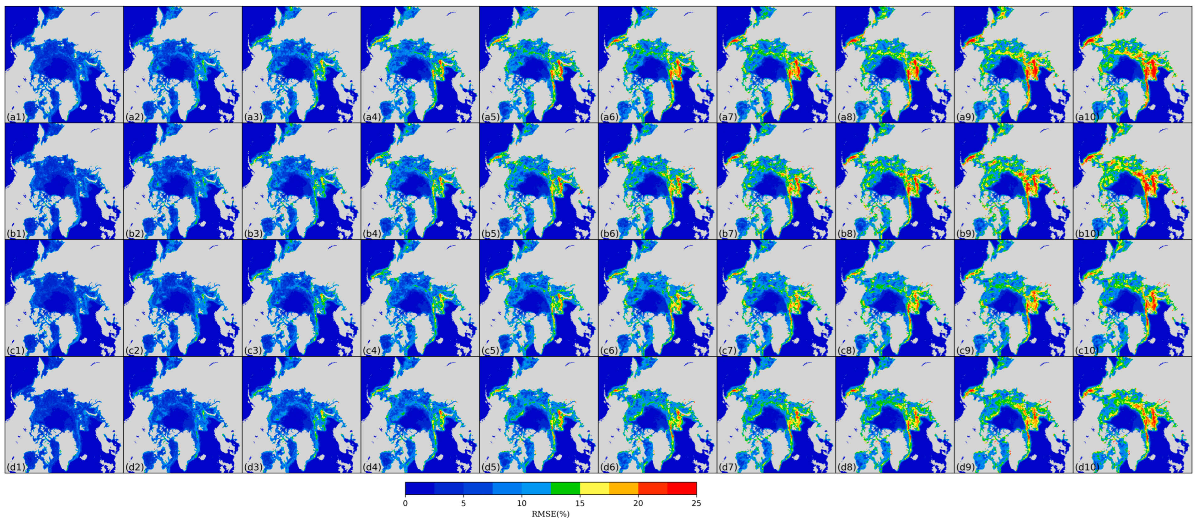
The RMSE of the daily scale SIC predicted values of the four models in 2020–2021 changes with the prediction time, as shown in Figure 7. The prediction error is concentrated within the one-year ice region, with minimal error observed in the multi-year ice region. Specifically, RMSE values initially rise in the Kara Sea and Barents Sea, followed by a gradual increase in the Laptev Sea and East Siberian Sea. The ConvLSTM-multi model demonstrates superior performance, displaying the slowest increase in RMSE with respect to the number of prediction days, particularly in the Kara Sea and Barents Sea. The inflow of warm salt water from the Atlantic Ocean[32,33] and positive solar radiation accumulated in summer[34] caused the sea ice in Kara Sea and Barents Sea to shrink, and the SIC to change rapidly, so the model prediction error of these two sea areas was large. There is annual sea ice drift from the Laptev Sea and East Siberian Sea to Fram Strait[35,36], which causes the sea ice along the line to change rapidly, and correspondingly increases the prediction error of the model along the line.

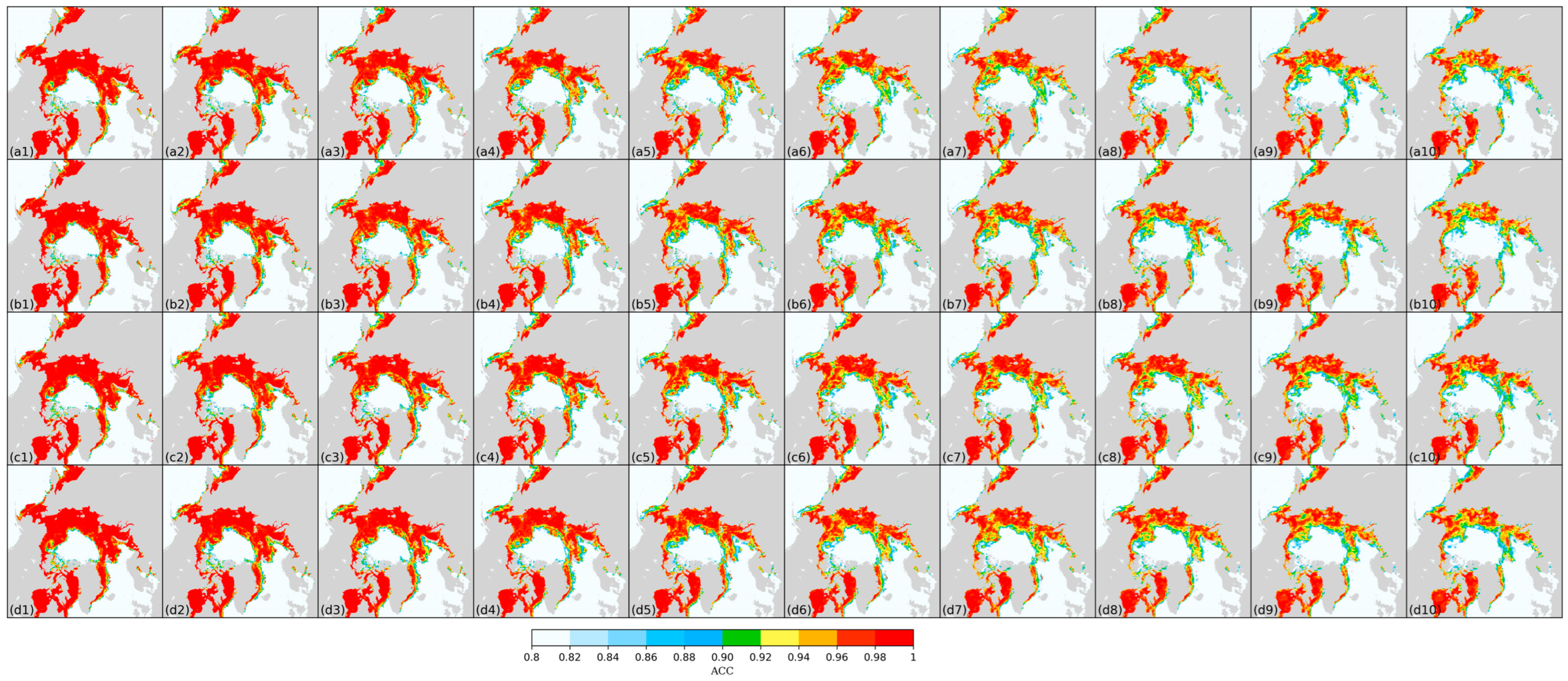
The ACC spatial distribution of the daily scale SIC predicted values of the four models in 2020 -2021 changes with the prediction time, as shown in Figure 8. The ACC of the one-year ice region is high, which shows that the anomalies predicted by the model are in good agreement with those observed in practice, and the model demonstrates its efficacy in accurately capturing the dynamic transition from sea ice melting to regrowth within the one-year ice region. SIC in the perennial ice area remains stable throughout the year, and the prediction error is small, so the ACC value is low. With the increase in forecast days, the consistency between the forecast anomaly and the observation anomaly in a year's ice area decreases. The ConvLSTM-multi model exhibits the highest performance, and the ACC of its prediction results decreases the slowest with the number of prediction days.

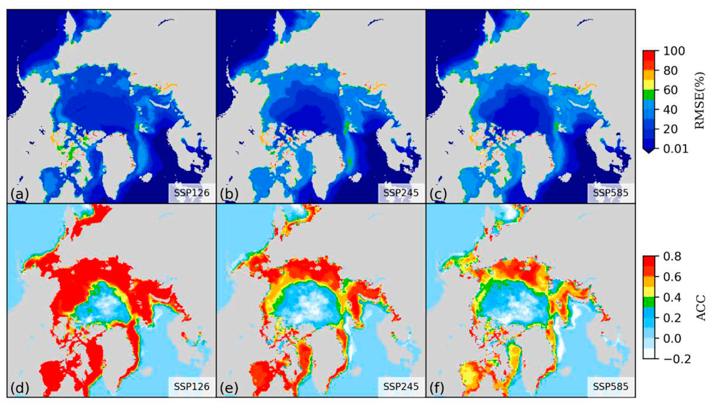
Figure A1 shows the RMSE and ACC of the "selected models" in CMIP6 for three future CO2 emission scenarios (SSP126, SSP245, and SSP585), with the RMSE of the predicted values in the SSP126 scenario being the best, and the RMSE of the predicted values for the one-year ice ranging from 20% to 50%, while the RMSE of the predicted values of the four models in the 10th day of the one-year ice ranges from 12.5% to 25%, indicating that the deep learning models can better predict the process of sea ice from melting to regrowth in the one-year ice. The ACC of the predicted values in the SSP126 scenario is optimal and is mainly distributed between 0.7 and 0.8 in the one-year ice, whereas the ACC of the predicted values of the four models on day 10 in the one-year ice region is mainly distributed between 0.9 and 1, which indicates that the deep learning models are more capable of predicting the anomalies that need to be captured.

3.2. Sea ice edge prediction accuracy

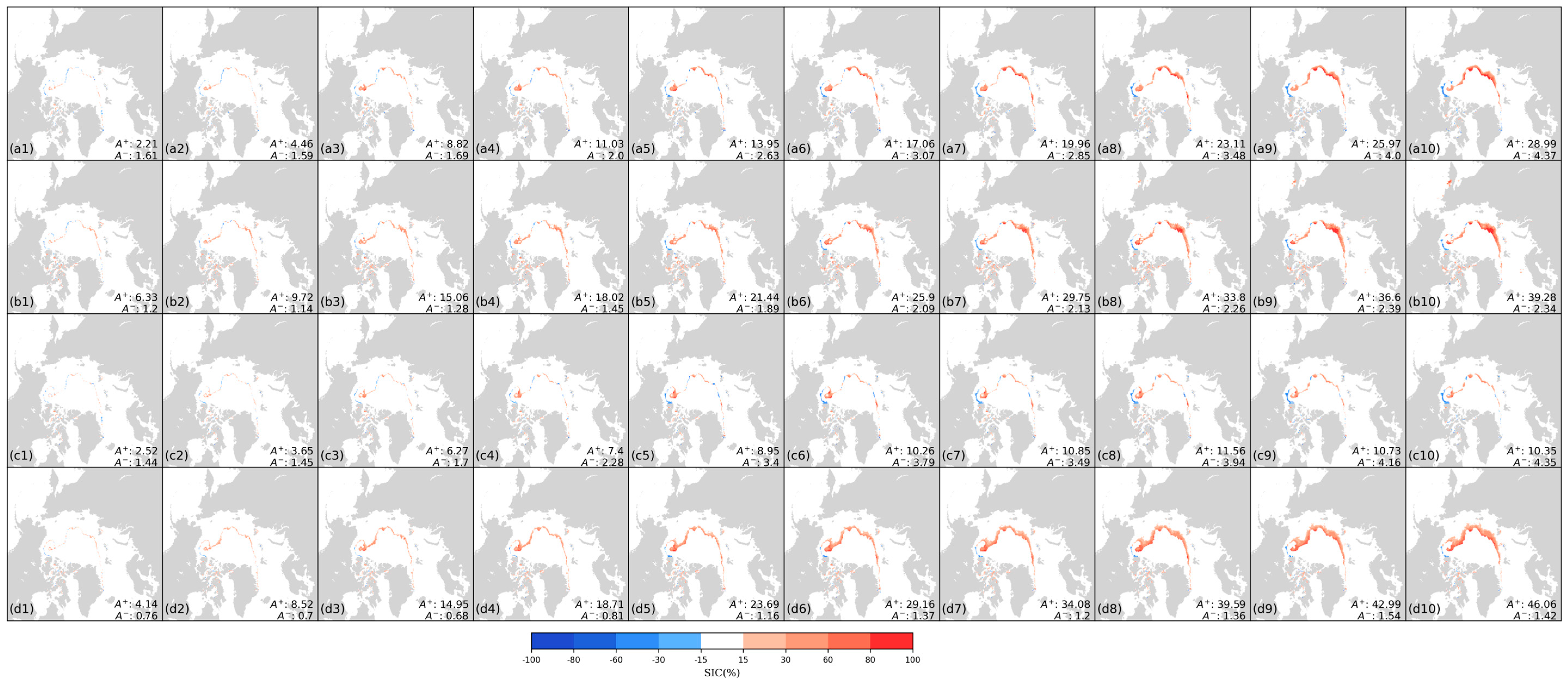
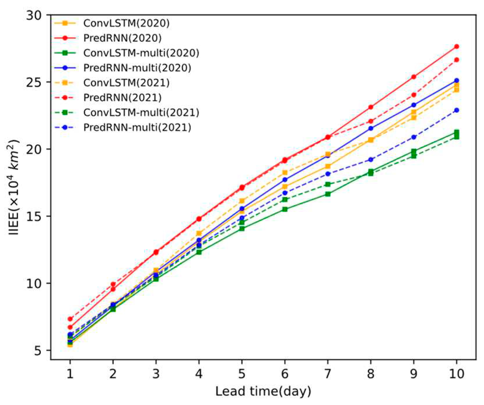
Figure 9 shows how the IIEE values of the four models change with the prediction time, and the IIEE values of the ConvLSTM-multi model increase the slowest with the prediction time. By contrasting the predictive outcomes of the ConvLSTM model with those of the ConvLSTM model supplemented with reanalysis data in the training dataset, it becomes evident that the inclusion of reanalysis data effectively enhances predictive accuracy for the sea ice edge region and mitigates the decline in accuracy as the prediction time lengthens. Similarly, the incorporation of reanalysis data in the PredRNN model also bolsters predictive accuracy for the sea ice edge region. In the extreme year (2020), the PredRNN-multi model yields higher IIEE values in predictions compared to the ConvLSTM model, while in the standard year (2021), it delivers lower values. This implies that the PredRNN-multi model falls short of matching the predictive capabilities of the ConvLSTM-multi model in thin ice region forecasting. Figure A3 provides a visual representation of the spatial distribution of IIEE for the four SIC prediction models for the period September 6-15, 2020, using SIC=15% as the threshold for distinguishing over-predicted ice regions (

A^{+}

) and under-predicted ice regions (

A^{-}

). The visual analysis corroborates that the ConvLSTM-multi model consistently demonstrates superior performance by exhibiting the least pronounced increase in IIEE values as the prediction time extends.

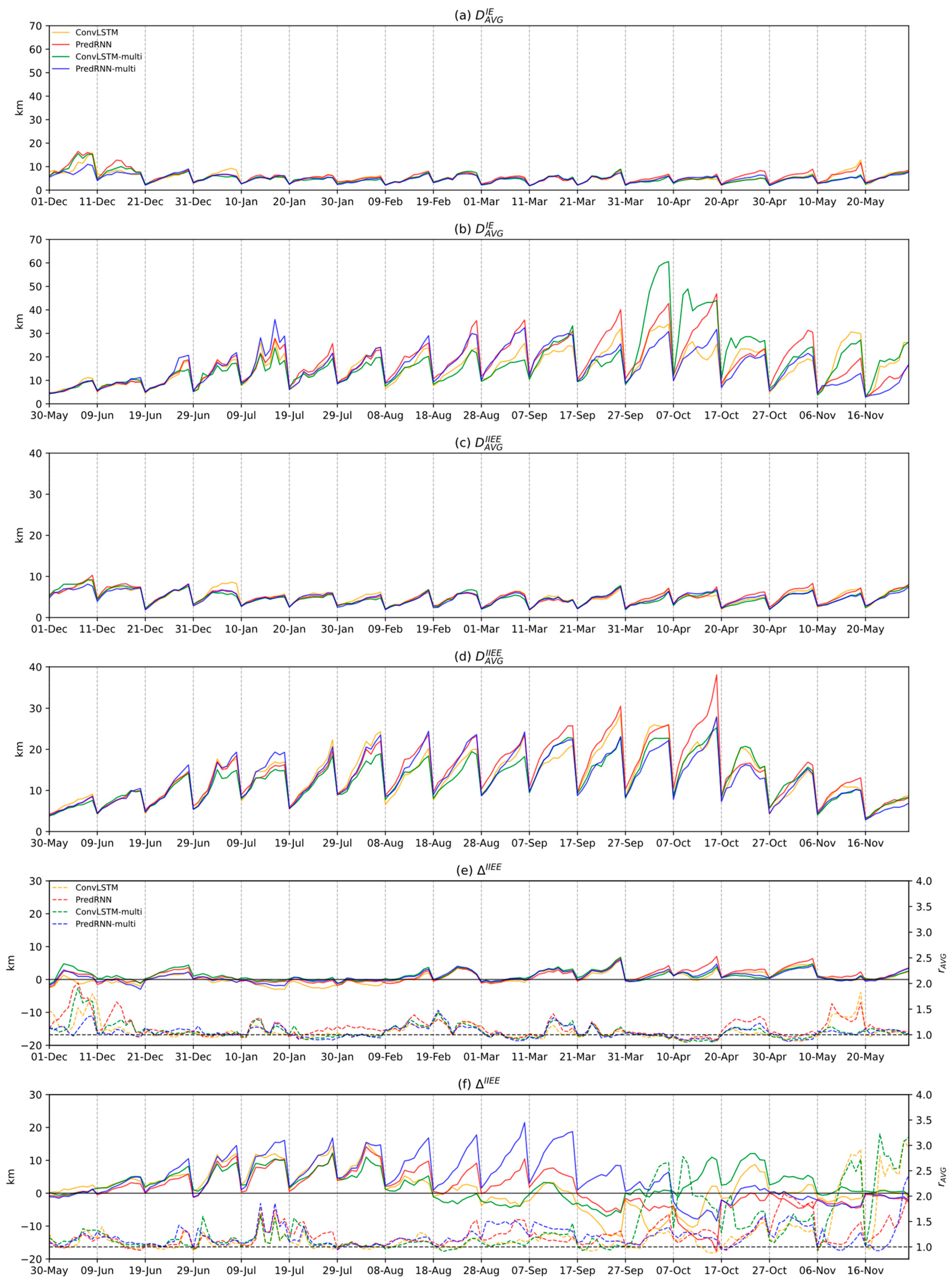
Figure 10 shows the distribution of

D_{AVG}^{IE}

D_{AVG}^{IIEE}

and

Δ^{IIEE}

across four model predictions during the winter–spring (freezing) and summer–autumn (melting) periods.

D_{AVG}^{IE}

is the point-to-point displacement between the predicted and observed ice edge, representing the upper limit of the sea-ice edge position displacements.

D_{AVG}^{IIEE}

represents the integral area displacement between the predicted and observed ice edge, delineating the lower limit of the sea-ice edge position displacement.

Δ^{IIEE}

quantifies the deviation in the predicted total ice content from the observed total ice content, and

γ_{A V G}

reflects the sensitivity of the actual error in the predicted ice-edge position concerning the applied displacement error measure. In the comparison of results from Figure 10 a, c, and e, it is evident that the deviation between the sea ice edge predicted by the four models during winter–spring and the observed values is minimal, exhibiting a gradual increase with the extension of the prediction time. Conversely, when contrasted with the outcomes from Figure 10b, d, and f, it becomes apparent that the deviation in the sea ice edge predicted by the four models during summer–autumn increases approximately three times faster than during winter–spring, and the trajectory of each index displays marked divergence. This discrepancy is primarily attributed to the more substantial changes in the sea ice edge area during summer–autumn, rendering predictions inherently more challenging. Analysis of the results from Figure 10 f reveals that the ConvLSTM model demonstrates a greater ability to anticipate the reduction in total sea ice content during the melting season compared to the PredRNN model. However, it exhibits inadequate learning capacity during the early stages of sea ice freezing (October–November). Referring to the sea ice edge displacement results presented in Table 3, the ConvLSTM-multi model exhibits superior performance during summer–autumn, while the PredRNN-multi model excels during spring–winter. Moreover, the mean values of

D_{AVG}^{IE}

D_{AVG}^{IIEE}

, and

| Δ^{IIEE} |

for the four models during both winter–spring and summer–autumn in 2021 surpass those of the CMIP6 models within the "selected models". The accuracy of the four models in predicting the sea ice edge's location is notably superior during winter–spring when compared to summer–autumn, as well as in contrast to the CMIP6 model.

3.3. Parameter Sensitivity Analysis

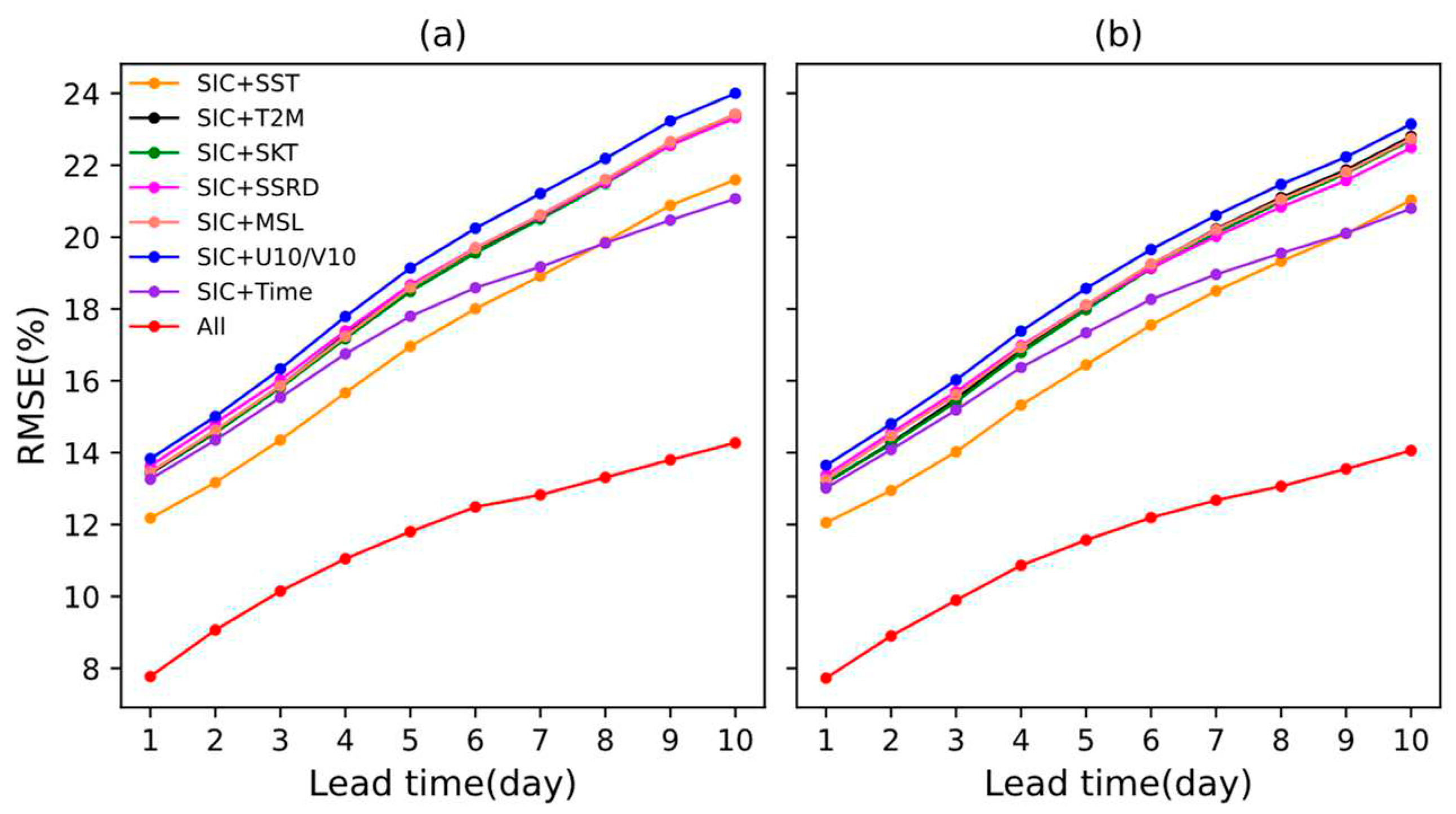
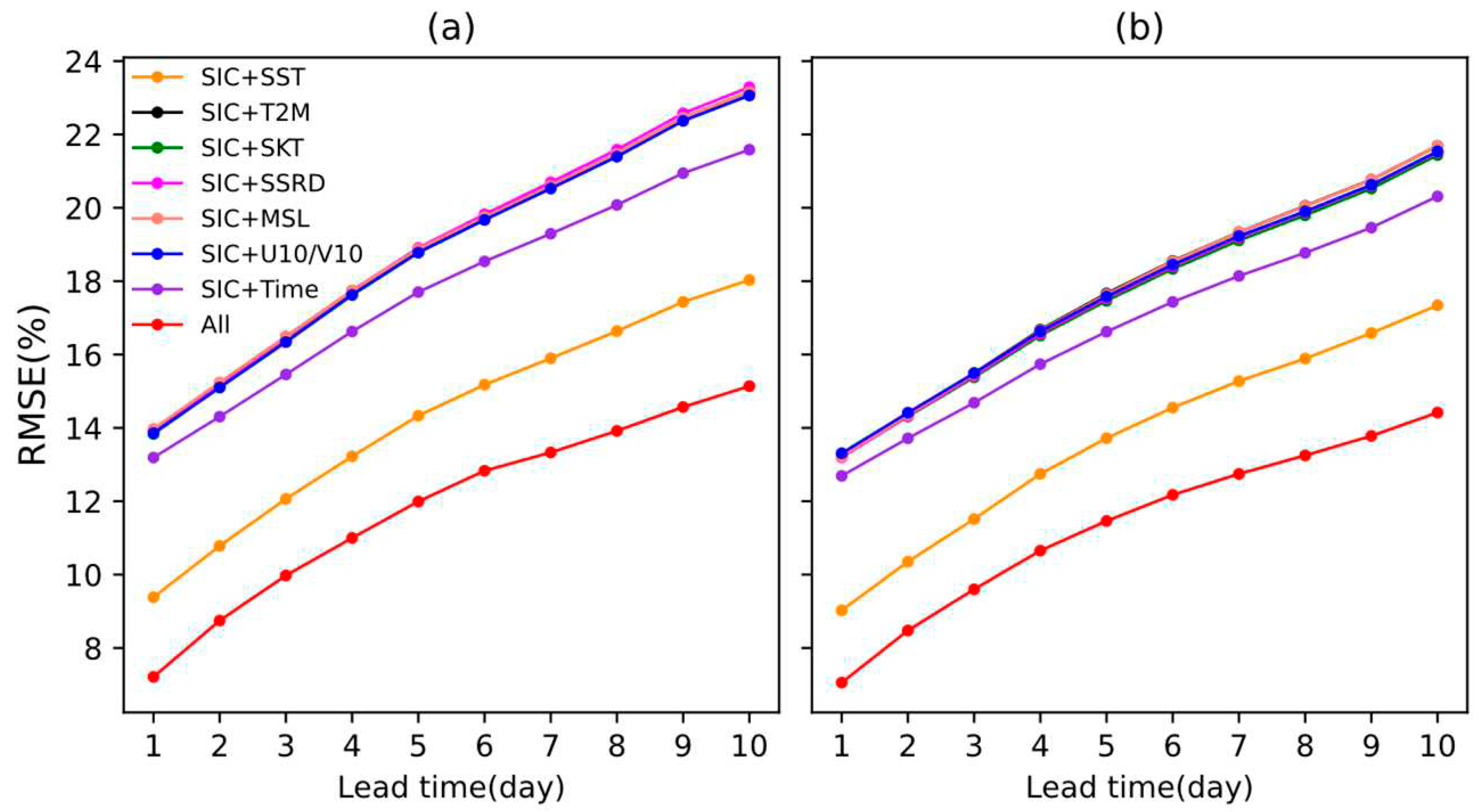
Examining the sensitivity of model prediction results to input parameters contributes to enhancing the selection of model input variables and improving prediction accuracy and efficiency. To assess the influence of specific parameters, the target parameters and SIC are retained, while all other parameters are replaced with noise. The RMSE is then for the model's predicted values. Comparative analysis of the RMSE values generated by different parameter types offers insights into the significance of each parameter's impact on the model's predictions. Smaller RMSE values indicate a stronger influence of the parameter on the model's predictive accuracy. Figure 11 and Figure 12 depict the RMSE distributions of prediction results for various input parameters in the ConvLSTM-multi and PredRNN-multi models. SST exhibits the most pronounced influence on model accuracy, followed by date. Notably, the PredRNN-multi model displays heightened sensitivity to SST in comparison to the ConvLSTM-multi model, while the ConvLSTM-multi model exhibits greater sensitivity to date than the PredRNN-multi model. Additionally, the ConvLSTM-multi model demonstrates a slight but noticeable sensitivity to parameters like T2M, SKT, SSRD, and MSL, with slightly more sensitivity to these parameters than to the U10/V10. In contrast, the PredRNN-multi model shows consistent sensitivity to T2M, SKT, SSRD, MSL, and U10/V10.

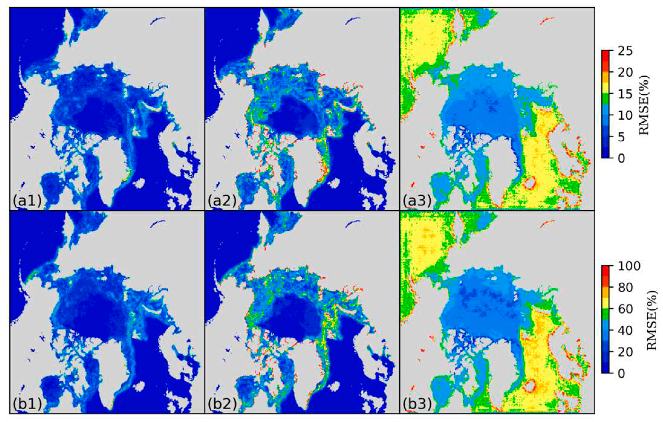
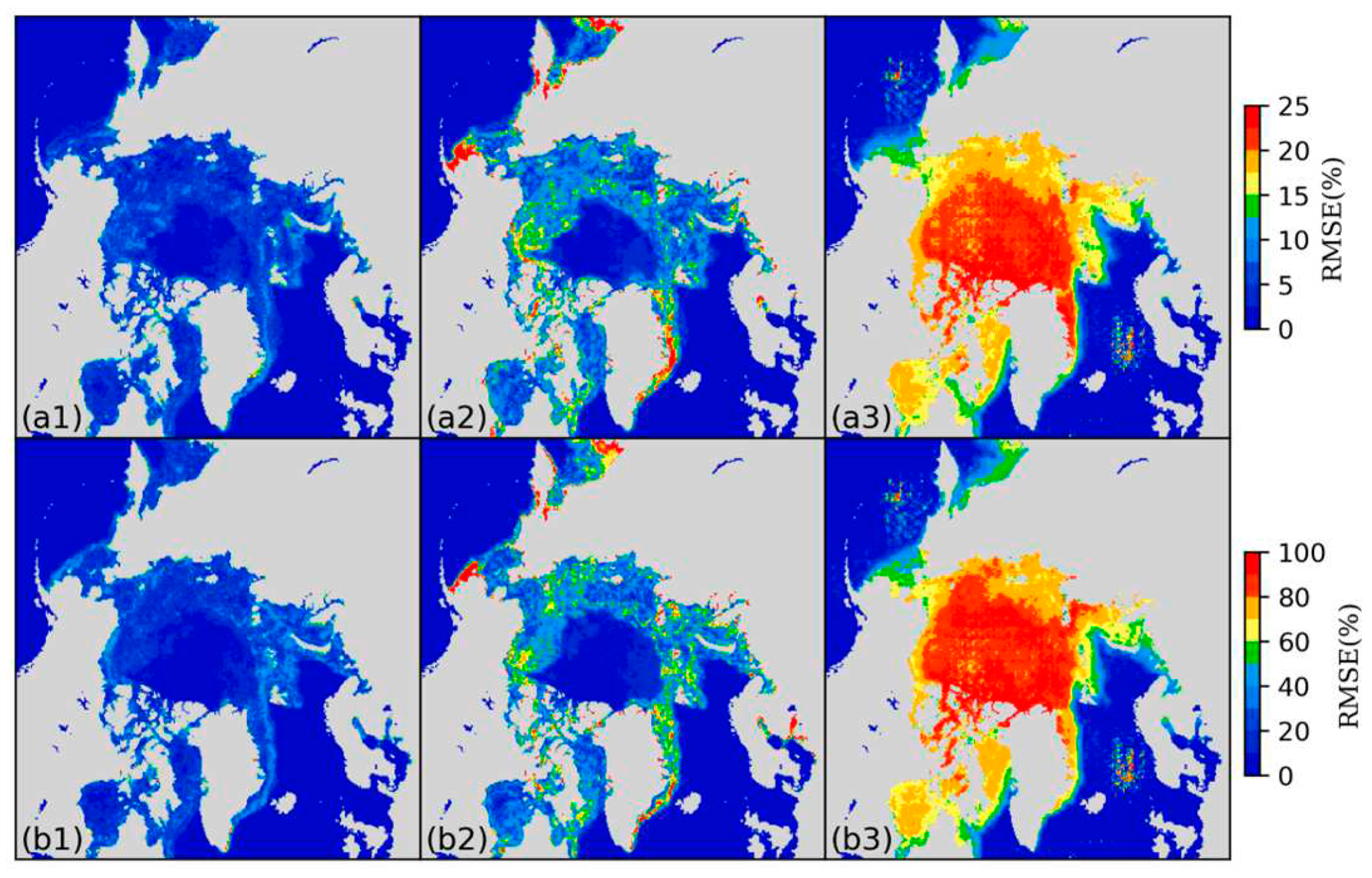
Comparison of RMSE distributions for the first-day SIC predictions reveals insights into the influence of input parameters on model predictions. This assessment is conducted under three scenarios: when no noise is introduced into the two models, when reanalysis data are treated as noise, and when SIC is considered as noise, Figure 13 and Figure 14 illustrate the outcomes. When meteorological data are treated as noise, both the ConvLSTM-multi and PredRNN-multi models exhibit challenges in accurately predicting the extent of thin ice near the sea ice edge. Notably, the PredRNN-multi model is more affected, aligning with the prior observation that this model displays heightened sensitivity to SST. On the other hand, the response of these models differs when input SIC are noisy. In the case of the ConvLSTM-multi model, the ice-free region's characteristics exert a more significant impact than those of the sea ice region. This outcome is attributed to the model's capacity to learn from the SIC, subsequently isolating the ice-free regions. In contrast, the PredRNN-multi model is primarily influenced by the sea ice region, with minimal impact observed in the ice-free region. This phenomenon arises from the model's ability to glean predictive insights from the distribution of sea ice within the SIC.

3.4. Prediction ability of the model under extreme conditions

Since the commencement of SIC data recording by the NSIDC, the Arctic's sea ice area in September reached historic lows in 2012 and 2020. To ensure the continuity and adequacy of the model's training data, the data from 2020 and 2021 are reserved for testing to evaluate the model's predictive performance in both extreme and normal years. In Figure 4a and 4b, the prediction accuracy of the four models for 2020 is behind that for 2021, with the ConvLSTM-multi model exhibiting superior predictive capabilities for the abrupt changes in September 2020's sea ice area. Figure 5 and Figure 6reveal a decrease in the grid count for high-value SIC from June to September 2020, with values approaching 0%. Notably, low-value SIC in 2020 was significantly less than in 2021. Consequently, metrics such as normalized nRMSE, ACC, NSE, and SSIM, which are sensitive to sea-ice edge prediction accuracy, performed better in 2020 compared to 2021 (Figure 4c-f). ComparingFigure 5d and Figure 6d, the PredRNN-multi model tends to overestimate SIC values from June to September 2020, primarily in the range of 95% to 100%, while its underestimating of values tends to be clustered around 0%. This indicates that the PredRNN-multi model falls short in predicting the sharp decline in the sea ice area in 2020, which also elucidates the significant difference in IIEE values between its 2020 and 2021 predictions (Figure 9). Conversely, the ConvLSTM-multi model's IIEE values for SIC predictions in 2020 and 2021 closely align with each other and exhibit less sensitivity to extreme years. Additionally, in Figure 11, Figure 12, Figure 13 and Figure 14, the trends in prediction accuracy corresponding to various input parameters in relation to prediction duration and spatial distribution remain consistent across different years, suggesting that the influence of input parameters on the model remains largely independent of yearly variations.

4. Conclusions

This study explores the integration of multiple predictors into the ConvLSTM and PredRNN models, thereby creating ConvLSTM-multi and PredRNN-multi models. These models are designed for the 10-day prediction of SIC across the entire Arctic Ocean. The findings underscore that the incorporation of meteorological reanalysis data within the ConvLSTM and PredRNN models leads to a significant enhancement in the daily scale prediction accuracy of SIC. Notably, the predictive accuracy of the model is most influenced by SST, followed by the date of SIC. The ConvLSTM-multi model demonstrates the lowest MAE, RMSE and IIEE, with the least increase with the extension in the prediction time. Moreover, the ConvLSTM-multi model exhibits commendable accuracy, particularly during extreme years, albeit with a slightly inferior performance in predicting the distribution of SIC values compared to the PredRNN-multi model. The evaluation of sea-ice edge displacement indicates that the ConvLSTM-multi model excels during summer and autumn, while the PredRNN-multi model performs optimally during spring and winter. Consequently, this comparative analysis highlights that the ConvLSTM-multi model is better suited for predicting SIC over the next 10 days.

Despite the progress made in this study, it is essential to acknowledge several limitations inherent to the model. The predictive capacity for SIC hinges on both the quantity of available SIC datasets and the diversity of input parameters. However, the quantity of SIC datasets and the spatial resolution offered by NSIDC are constrained, necessitating a higher volume of datasets to further refine the model's parameters. Additionally, the model exhibits limited predictive capability for summer sea ice due to its exclusive reliance on reanalysis data. Crucial parameters such as sea ice thickness and ice melting pools, which wield a substantial influence on sea ice dynamics, have not been incorporated into the model. This omission can be attributed to the limited availability and accessibility of these parameters. Lastly, the study falls short in comprehensively analyzing the impact of input parameters on prediction outcomes and discerning the intricate nonlinear relationships between them. Future research endeavors will focus on intensifying the analysis of physical parameters influencing sea ice variations and enhancing the model's capacity to assimilate input data, to enhance the prediction ability of the model.

Author Contributions

Conceptualization, J.L. and J.F.; methodology, J.F.; software, J.F.; validation, J.F., J.L. and W.Z.; formal analysis, J.F.; investigation, J.L. and J.F.; resources, J.L., J.F., W.Z. and Z.L.; data curation, J.F., J.W., Z.L., L.K. and L.G.; writing—original draft preparation, J.F., J.L. and L.G.; writing—review and editing, J.L.; visualization, J.F. and J.W.; supervision, J.L.; project administration, J.L.; funding acquisition, J.L. All authors have read and agreed to the published version of the manuscript.

Funding

This work was supported by the National Natural Science Foundation of China (42374053), the Hunan Provincial Natural Science Foundation of China (2023JJ30656).

Data Availability Statement

Sea ice concentration data (Bootstrap Sea Ice Concentrations from Nimbus-7 SMMR and DMSP SSM/I-SSMIS, Version 3) are available from the National Snow and Ice Data Center (NSIDC) and Information System(https://nsidc.org). ERA5 hourly data (ERA5 hourly data on single levels from 1940 to present) are available from the European Centre for Medium-Range Weather Forecasts (ECMWF) and Information System(https://cds.climate.copernicus.eu). The CMIP6 models and the multi-realizations are available from the World Climate Research Programme (WCRP) and Information System (https://esgf-node.llnl.gov/search/cmip6).

Acknowledgments

The authors would like to thank the National Snow and Ice Data Center and the European Centre for Medium-Range Weather Forecasts for providing open SIC data and ERA5 reanalysis data. We also extend our sincere gratitude to jhhuang96 for sharing the ConvLSTM Model code on GitHub (https://github.com/jhhuang96/ConvLSTM-PyTorch) and to Haixu Wu for sharing the PredRNN Model code on GitHub (https://github.com/thuml/predrnn-pytorch), which served as valuable references for our research.

Conflicts of Interest

The authors declare no conflict of interest.

Appendix A

Table A1. CMIP6 Models and realizations used in this study. The projections including SSP126, SSP245 and SSP585, are from 2020 to 2021 in this study.

Model	Spatial resolution	Frequency	Experiment (ensemble members)
ACCESS-CM2	360×300	day	SSP126(1)	r1i1p1f1	SSP245(1)	r1i1p1f1	SSP585(1)	r1i1p1f1
CESM2-WACCM	320×384	day	SSP126(1)	r1i1p1f1	SSP245(5)	r1i1p1f1	SSP585(5)	r1i1p1f1
						r2i1p1f1		r2i1p1f1
						r3i1p1f1		r3i1p1f1
						r4i1p1f1		r4i1p1f1
						r5i1p1f1		r5i1p1f1
MIROC6	360×256	day	SSP126(3)	r11p1f1	SSP245(3)	r1i1p1f1	SSP585(3)	r1i1p1f1
				r2i1p1f1		r2i1p1f1		r2i1p1f1
				r3i1p1f1		r3i1p1f1		r3i1p1f1
MRI-ESM2-0	360×364	day	SSP126(1)	r1i1p1f1	SSP245(1)	r1i1p1f1	SSP585(1)	r1i1p1f1

Figure A1. The distribution of RMSE(a-c) and ACC(d-f) of SIC in Arctic sea area in 2020-2021 predicted by the "selected models" in CMIP6 under three CO2 emission scenarios (SSP126, SSP245 and SSP585) in the future.

Figure A2. Observations (a1-a10) and predictions from the ConvLSTM (b1-b10), PredRNN (c1-c10), ConvLSTM-multi (d1-d10), and PredRNN-multi (e1-e10) models for the Arctic SIC on September 6-15, 2020. Gray represents land, dark blue represents ice-free ocean, and the red line is the sea ice boundary for observations and the green line is the sea ice boundary predicted by the model. SIC=15% is the sea ice boundary. The ACC and sea ice area (SIE) errors of the four models' daily predictions are shown in the lower right corner.

Figure A3. IIEE distribution of predicted SIC of four models from September 6 to 15, 2020. The red represents

A^{+}

, and the blue represents

A^{-}

A^{+}

and

A^{-}

in the lower right corner represent the areas of the multi-prediction and the under-prediction of the model (unit:

10^{4} k m^{2}

). (a1-a10), (b1-b10), (c1-c10) and (d1-d10) correspond to the IIEE distributions of ConvLSTM, PredRNN, ConvLSTM-multi and PredRNN-multi models from the first day to the tenth day.

Figure A3. IIEE distribution of predicted SIC of four models from September 6 to 15, 2020. The red represents

A^{+}

, and the blue represents

A^{-}

A^{+}

and

A^{-}

in the lower right corner represent the areas of the multi-prediction and the under-prediction of the model (unit:

10^{4} k m^{2}

). (a1-a10), (b1-b10), (c1-c10) and (d1-d10) correspond to the IIEE distributions of ConvLSTM, PredRNN, ConvLSTM-multi and PredRNN-multi models from the first day to the tenth day.

References

Serreze, M.C.; Meier, W.N. The Arctic's sea ice cover: trends, variability, predictability, and comparisons to the Antarctic. Annals of the New York Academy of Sciences 2019, 1436, 36–53. [Google Scholar] [CrossRef] [PubMed]
Cavalieri, D.J.; Parkinson, C.L. Arctic sea ice variability and trends, 1979-2010. Cryosphere 2012, 6, 881–889. [Google Scholar] [CrossRef]
Stroeve, J.C.; Serreze, M.C.; Holland, M.M.; Kay, J.E.; Malanik, J.; Barrett, A.P. The Arctic’s rapidly shrinking sea ice cover: a research synthesis. Climatic change 2012, 110, 1005–1027. [Google Scholar] [CrossRef]
Devasthale, A.; Sedlar, J.; Koenigk, T.; Fetzer, E. The thermodynamic state of the Arctic atmosphere observed by AIRS: comparisons during the record minimum sea ice extents of 2007 and 2012. Atmospheric Chemistry and Physics 2013, 13, 7441–7450. [Google Scholar] [CrossRef]
Wang, Y.H.; Bi, H.B.; Huang, H.J.; Liu, Y.X.; Liu, Y.L.; Liang, X.; Fu, M.; Zhang, Z.H. Satellite-observed trends in the Arctic sea ice concentration for the period 1979-2016. Journal of Oceanology and Limnology 2019, 37, 18–37. [Google Scholar] [CrossRef]
Witze, A. Arctic sea ice hits second-lowest level on record. Nature 2020. [CrossRef]
Stephen, K. Societal Impacts of a Rapidly Changing Arctic. Current Climate Change Reports 2018, 4, 223–237. [Google Scholar] [CrossRef]
Blanchard-Wrigglesworth, E.; Armour, K.C.; Bitz, C.M.; DeWeaver, E. Persistence and inherent predictability of Arctic sea ice in a GCM ensemble and observations. Journal of Climate 2011, 24, 231–250. [Google Scholar] [CrossRef]
Krikken, F.; Hazeleger, W. Arctic energy budget in relation to sea ice variability on monthly-to-annual time scales. Journal of Climate 2015, 28, 6335–6350. [Google Scholar] [CrossRef]
Guemas, V.; Blanchard-Wrigglesworth, E.; Chevallier, M.; Day, J.J.; Deque, M.; Doblas-Reyes, F.J.; Fuckar, N.S.; Germe, A.; Hawkins, E.; Keeley, S.; et al. A review on Arctic sea-ice predictability and prediction on seasonal to decadal time-scales. Quarterly Journal of the Royal Meteorological Society 2016, 142, 546–561. [Google Scholar] [CrossRef]
Mohammadi-Aragh, M.; Goessling, H.; Losch, M.; Hutter, N.; Jung, T. Predictability of Arctic sea ice on weather time scales. Scientific reports 2018, 8, 6514. [Google Scholar] [CrossRef] [PubMed]
Cruz-García, R.; Guemas, V.; Chevallier, M.; Massonnet, F. An assessment of regional sea ice predictability in the Arctic ocean. Climate dynamics 2019, 53, 427–440. [Google Scholar] [CrossRef]
Onarheim, I.H.; Eldevik, T.; Årthun, M.; Ingvaldsen, R.B.; Smedsrud, L.H. Skillful prediction of Barents Sea ice cover. Geophysical Research Letters 2015, 42, 5364–5371. [Google Scholar] [CrossRef]
Leppäranta, M.; Meleshko, V.P.; Uotila, P.; Pavlova, T. Sea Ice Modelling. In Sea Ice in the Arctic: Past, Present and Future, Johannessen, O.M., Bobylev, L.P., Shalina, E.V., Sandven, S., Eds.; Springer International Publishing: Cham, 2020; pp. 315-387.
Chi, J.; Kim, H.C. Prediction of Arctic Sea Ice Concentration Using a Fully Data Driven Deep Neural Network. Remote Sens. 2017, 9, 19. [Google Scholar] [CrossRef]
Choi, M.; De Silva, L.W.A.; Yamaguchi, H. Artificial Neural Network for the Short-Term Prediction of Arctic Sea Ice Concentration. Remote Sens. 2019, 11, 12. [Google Scholar] [CrossRef]
Kim, J.; Kim, K.; Cho, J.; Kang, Y.Q.; Yoon, H.J.; Lee, Y.W. Satellite-Based Prediction of Arctic Sea Ice Concentration Using a Deep Neural Network with Multi-Model Ensemble. Remote Sens. 2019, 11, 20. [Google Scholar] [CrossRef]
Fritzner, S.; Graversen, R.; Christensen, K.H. Assessment of High-Resolution Dynamical and Machine Learning Models for Prediction of Sea Ice Concentration in a Regional Application. J. Geophys. Res.-Oceans 2020, 125. [CrossRef]
Kim, Y.J.; Kim, H.C.; Han, D.; Lee, S.; Im, J. Prediction of monthly Arctic sea ice concentrations using satellite and reanalysis data based on convolutional neural networks. Cryosphere 2020, 14, 1083–1104. [Google Scholar] [CrossRef]
Andersson, T.R.; Hosking, J.S.; Perez-Ortiz, M.; Paige, B.; Elliott, A.; Russell, C.; Law, S.; Jones, D.C.; Wilkinson, J.; Phillips, T.; et al. Seasonal Arctic sea ice forecasting with probabilistic deep learning. Nature Communications 2021, 12. [Google Scholar] [CrossRef] [PubMed]
Liu, Y.; Bogaardt, L.; Attema, J.; Hazeleger, W. Extended-Range Arctic Sea Ice Forecast with Convolutional Long Short-Term Memory Networks. Mon. Weather Rev. 2021, 149, 1673–1693. [Google Scholar] [CrossRef]
Comiso, J.C. Bootstrap Sea Ice Concentrations from Nimbus-7 SMMR and DMSP SSM/I-SSMIS, Version 3. Available online: https://nsidc.org/data/NSIDC-0079/versions/3 (accessed on 6 5 2023).
Hersbach, H., Bell, B., Berrisford, P., Biavati, G., Horányi, A., Muñoz Sabater, J., Nicolas, J., Peubey, C., Radu, R., Rozum, I., Schepers, D., Simmons, A., Soci, C., Dee, D., Thépaut, J-N. ERA5 hourly data on single levels from 1940 to present. Copernicus Climate Change Service (C3S) Climate Data Store (CDS). Available online: https://cds.climate.copernicus.eu/cdsapp#!/dataset/10.24381/cds.adbb2d47?tab=form (accessed on 6 5 2023).
Arctic sea ice minimum is 2nd lowest on record. Available online: https://public.wmo.int/en/media/news/arctic-sea-ice-minimum-2nd-lowest-record (accessed on 6 7 2023).
Notz, D.; Community, S. Arctic sea ice in CMIP6. Geophysical Research Letters 2020, 47, e2019GL086749. [Google Scholar] [CrossRef]
Shi, X.J.; Chen, Z.R.; Wang, H.; Yeung, D.Y.; Wong, W.K.; Woo, W.C. Convolutional LSTM Network: A Machine Learning Approach for Precipitation Nowcasting. In Proceedings of the 29th Annual Conference on Neural Information Processing Systems (NIPS), Montreal, CANADA, Dec 07-12, 2015.
Wang, Y.; Wu, H.; Zhang, J.; Gao, Z.; Wang, J.; Yu, P.; Long, M. PredRNN: A Recurrent Neural Network for Spatiotemporal Predictive Learning. IEEE transactions on pattern analysis and machine intelligence 2022, PP.
Sutskever, I.; Vinyals, O.; Le, Q.V. Sequence to sequence learning with neural networks. Advances in neural information processing systems 2014, 27. [Google Scholar]
Bengio, S.; Vinyals, O.; Jaitly, N.; Shazeer, N. Scheduled Sampling for Sequence Prediction with Recurrent Neural Networks. In Proceedings of the 29th Annual Conference on Neural Information Processing Systems (NIPS), Montreal, CANADA, Dec 07-12, 2015.
Melsom, A.; Palerme, C.; Müller, M. Validation metrics for ice edge position forecasts. Ocean Sci. 2019, 15, 615–630. [Google Scholar] [CrossRef]
Goessling, H.F.; Tietsche, S.; Day, J.J.; Hawkins, E.; Jung, T. Predictability of the Arctic sea ice edge. Geophysical Research Letters 2016, 43, 1642–1650. [Google Scholar] [CrossRef]
Schauer, U.; Loeng, H.; Rudels, B.; Ozhigin, V.K.; Dieck, W. Atlantic water flow through the Barents and Kara Seas. Deep Sea Research Part I: Oceanographic Research Papers 2002, 49, 2281–2298. [Google Scholar] [CrossRef]
Årthun, M.; Eldevik, T.; Smedsrud, L.; Skagseth, Ø.; Ingvaldsen, R. Quantifying the influence of Atlantic heat on Barents Sea ice variability and retreat. Journal of Climate 2012, 25, 4736–4743. [Google Scholar] [CrossRef]
Stroeve, J.C.; Serreze, M.C.; Holland, M.M.; Kay, J.E.; Malanik, J.; Barrett, A.P. The Arctic's rapidly shrinking sea ice cover: a research synthesis. Climatic change 2012, 110, 1005. [Google Scholar] [CrossRef]
Pfirman, S.; Colony, R.; Nürnberg, D.; Eicken, H.; Rigor, I. Reconstructing the origin and trajectory of drifting Arctic sea ice. Journal of Geophysical Research: Oceans 1997, 102, 12575–12586. [Google Scholar] [CrossRef]
Pavlov, V.; Pavlova, O.; Korsnes, R. Sea ice fluxes and drift trajectories from potential pollution sources, computed with a statistical sea ice model of the Arctic Ocean. Journal of marine Systems 2004, 48, 133–157. [Google Scholar] [CrossRef]

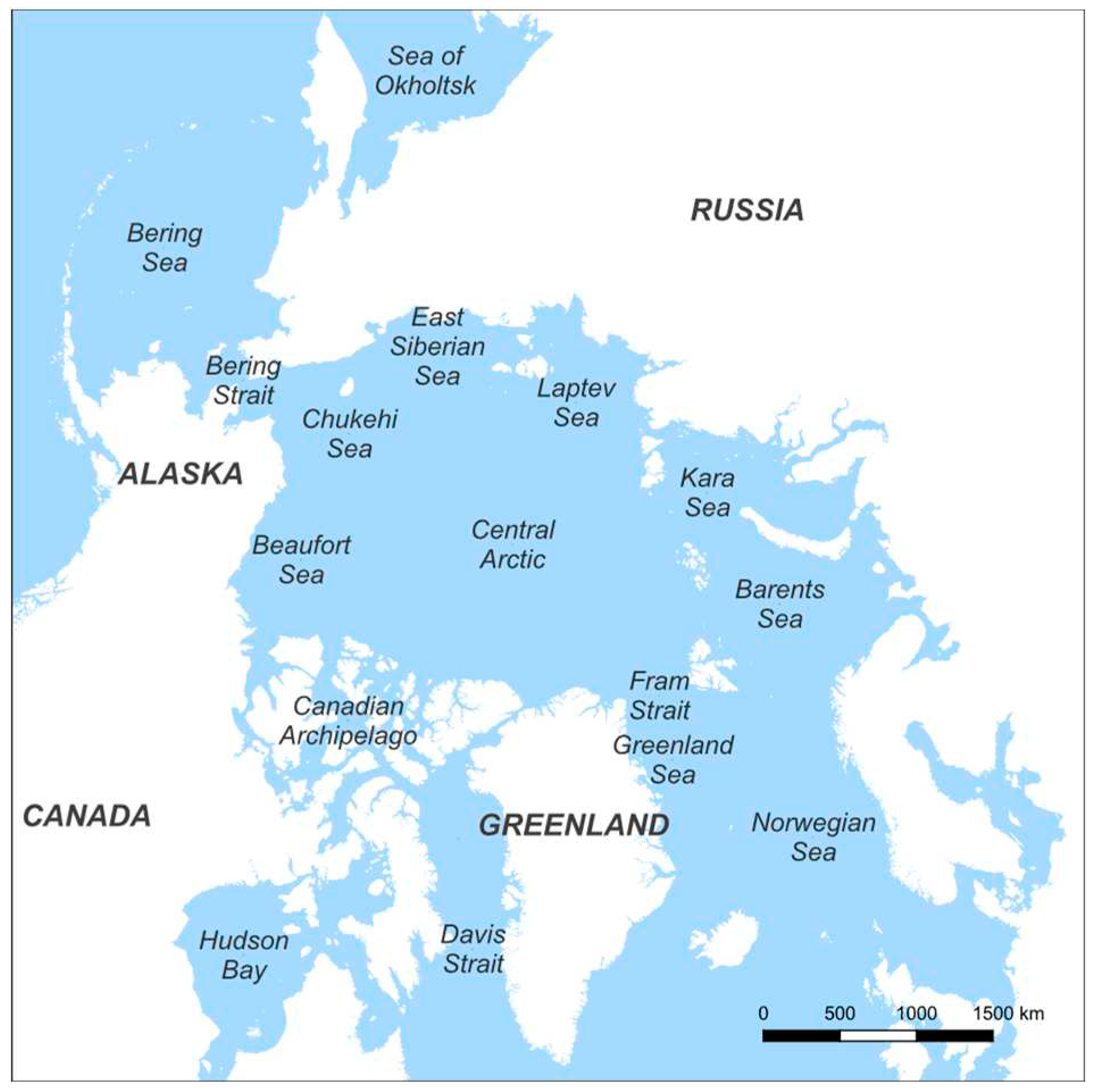
Figure 1. Distribution map of sea in the study area.

Figure 2. The convolutional LSTM (ConvLSTM) network framework.

Figure 3. The predictive recurrent neural network (PredRNN) network framework.

Figure 4. ConvLSTM, PredRNN, ConvLSTM-multi, and PredRNN-multi models' SIC prediction accuracies over prediction time in 2020 and 2021.

Figure 5. Histograms of NSIDC SIC versus four model predictions during the melt season (June-September 2020). (a), (b), (c), and (d) corresponding to ConvLSTM, PredRNN, ConvLSTM-multi, and PredRNN-multi, respectively.

Figure 6. Histograms of NSIDC SIC versus four model predictions during the melt season (June-September 2021). (a), (b), (c), and (d) corresponding to ConvLSTM, PredRNN, ConvLSTM-multi, and PredRNN-multi, respectively.

Figure 7. The change in RMSE of daily scale SIC forecast values of four models from 2020 to 2021 with the increase in forecast days. (a1-a10), (b1-b10), (c1-c10) and (d1-d10), respectively, correspond to the RMSE distributions of ConvLSTM, PredRNN, ConvLSTM-multi and PredRNN-multi models from the first day to the tenth day.

Figure 8. The change in ACC of daily scale SIC forecast values of four models from 2020 to 2021 with the increase in forecast days. (a1-a10), (b1-b10), (c1-c10) and (d1-d10), respectively, correspond to the ACC distributions of ConvLSTM, PredRNN, ConvLSTM-multi and PredRNN-multi models from the first day to the tenth day.

Figure 9. The change in the integrated ice edge error (IIEE) values of the four model predictions over the prediction time, (a) and (b) represent the years 2020 and 2021, with IIEE in

{km}^{2}

Figure 9. The change in the integrated ice edge error (IIEE) values of the four model predictions over the prediction time, (a) and (b) represent the years 2020 and 2021, with IIEE in

{km}^{2}

Figure 10. a-b, c-d, and e-f represent the average displacement of the ice edge (

D_{AVG}^{IE}

), the average displacement of the integrated ice edge error (

D_{AVG}^{IIEE}

), and the deviation in the integrated ice edge error (

Δ^{IIEE}

) for the four models in 2021, respectively, and the dashed lines in e and f correspond to the

r_{A V G}

of the four models.

Figure 10. a-b, c-d, and e-f represent the average displacement of the ice edge (

D_{AVG}^{IE}

), the average displacement of the integrated ice edge error (

D_{AVG}^{IIEE}

), and the deviation in the integrated ice edge error (

Δ^{IIEE}

) for the four models in 2021, respectively, and the dashed lines in e and f correspond to the

r_{A V G}

of the four models.

Figure 11. RMSE distribution of the prediction results corresponding to different input parameters of the ConvLSTM-multi model. The red line represents the prediction results with all the input parameters. (a) and (b) correspond to the model predictions for 2020 and 2021, respectively.

Figure 12. RMSE distribution of the prediction results corresponding to different input parameters of the PredRNN-multi model. The red line represents the prediction results of inputting all parameters. (a) and (b) correspond to the model predictions for 2020 and 2021, respectively.

Figure 13. RMSE distributions of the first day SIC predictions for the ConvLSTM-multi model without adding any noise (a1), (b1), masking the reanalysis data as noise (a2), (b2) and masking the SIC as noise (c1), (c2). a1-a3 and b1-b3 correspond to the predicted values for 2020 and 2021, respectively.

Figure 14. RMSE distributions of the first day SIC predictions for the PredRNN-multi model without adding any noise (a1), (b1), masking the reanalysis data as noise (a2), (b2) and masking the SIC as noise (c1), (c2). a1-a3 and b1-b3 correspond to the predicted values for 2020 and 2021, respectively.

Table 1. The specifications of the eleven predictors used to predict short-term sea ice concentration (SIC) in the study.

Variable	Source	Unit	Temporal resolution		Value range
Sea ice concentration	NSIDC	%	Daily	25 km	[0,1]
Sea surface temperature	ECMWF ERA5	K	Hourly	0.25°	[0,1]
2m temperature	ECMWF ERA5	K	Hourly	0.25°	[0,1]
Skin temperature	ECMWF ERA5	K	Hourly	0.25°	[0,1]
Surface solar radiation downwards	ECMWF ERA5	J m-2	Hourly	0.25°	[0,1]
Mean sea level pressure	ECMWF ERA5	Pa	Hourly	0.25°	[0,1]
10m u-component of wind	ECMWF ERA5	m s-1	Hourly	0.25°	[0,1]
10m v-component of wind	ECMWF ERA5	m s-1	Hourly	0.25°	[0,1]
Land mask	#	#	Daily	25 km	0/1
Cosine of initialization day index	#	#	Daily	25 km	[–1,1]
Sine of initialization day index	#	#	Daily	25 km	[-1,1]

Table 2. The daily average prediction accuracy of SIC in 2020 and 2021 by the "selected models" in CMIP6 under three CO2 emission scenarios (SSP126, SSP245 and SSP585).

Year	Scenarios	MAE	RMSE	nRMSE	ACC	NSE
2020	SSP126	19.67%	29.13%	69%	0.76	0.53
	SSP245	23.57%	32.94%	78%	0.74	0.47
	SSP585	25.44%	35.2%	85%	0.71	0.41
2021	SSP126	20.08%	29.22%	70%	0.76	0.53
	SSP245	23.32%	32.11%	76%	0.75	0.49
	SSP585	24.58%	33.95%	80%	0.73	0.45

Table 3. Average sea ice edge displacement (unit: km) in winter–spring and summer–autumn of 2021 under three future CO2 emission scenarios (SSP126, SSP245, and SSP585) for the four deep learning models in this study and the "selected models" in CMIP6.

	ConvLSTM		PredRNN		ConvLSTM-multi		PredRNN-multi		SSP126		SSP245		SSP585
$D_{AVG}^{IE}$	5.44	14.97	6.28	18.10	5.45	15.51	5.05	16.86	30.50	127.46	28.74	203.26	30.85	217.10
$D_{AVG}^{IIEE}$	5.03	12.51	5.15	13.72	4.87	11.74	4.79	13.52	25.18	90.62	23.32	124.80	23.36	132.34
$\| Δ^{IIEE} \|$	1.42	4.70	1.68	5.68	1.55	4.39	1.36	7.73	6.92	66.94	2.62	111.80	3.54	118.79
$r_{A V G}$	1.07	1.22	1.19	1.27	1.10	1.31	1.05	1.23	1.22	1.4	1.24	1.54	1.33	1.56

Disclaimer/Publisher’s Note: The statements, opinions and data contained in all publications are solely those of the individual author(s) and contributor(s) and not of MDPI and/or the editor(s). MDPI and/or the editor(s) disclaim responsibility for any injury to people or property resulting from any ideas, methods, instructions or products referred to in the content.

© 2023 by the authors. Licensee MDPI, Basel, Switzerland. This article is an open access article distributed under the terms and conditions of the Creative Commons Attribution (CC BY) license (http://creativecommons.org/licenses/by/4.0/).

Copyright: This open access article is published under a Creative Commons CC BY 4.0 license, which permit the free download, distribution, and reuse, provided that the author and preprint are cited in any reuse.

MDPI Initiatives

Important Links

Choose an area of interest and we will send you notifications of new preprints at your preferred frequency.

Disclaimer

Daily Scale Prediction of Arctic Sea Ice Concentration Based on Recurrent Neural Network Models

Abstract