1. Introduction
Artworks are subjected to structural changes from environmental alterations due to relative humidity (RH) fluctuations. These variations, usually, have a short-term transition in hourly rate, but they may accumulate and cause long-term impact on structural condition of the artworks. So, they in turn are causing conservation problems especially due to the difference of the artworks painting technique (pigments, binding material) and its support (wall, wood, canvas etc) where the alterations mainly occur to. Concerning paintings, the wood as a support appeared before canvas, and a lot of famous paintings were made on wood (The Mona Lisa from Leonardo da Vinci, The Virgin and Child with Saint John the Baptist (La Belle Jardinière) from Raphael).
Wood is an organic material with hydrophilic properties, meaning that wood support is sensitive to RH changes. The reaction of wood to climate changes depends on the wood’s anatomical direction (i.e. axial, radial, and tangential), dimensions and species. For example, an oak panel with a radial cut will be less altered by the environment changes than a pin panel with tangential cut with the same environmental conditions. This statement does not take into account the history of the wooden panel such as worm galleries or structural problems, for example nodes.
There are common understandings on wood mechanisms which have been thoroughly studied by wood experts and material scientists. They agree that RH increasing induce an increase of moisture exchanges between wood objects and its environment. These exchanges are causing more movement of the wood, creating more opportunity for defects to appear in the wood. The defects created during continuous processes of RH variations have almost not been experimentally verified.
Signs of early failure have never been experimentally detected or proven by a contactless method, especially in materials as complex as wooden panels. It implies a difference in reactions between wood alone and those objects of art. The behaviour of the object will depend on the wood species, thickness, age and history and the nature of the layers, (the panel has varnish, etc.). Nonetheless, experiments on wood have been conducted to detect early cracks using acoustic emission [
1,
2]. The acoustic sensors are usually in contact with the artworks to have a better signal and the information given by those sensors are pointwise. A method contactless and taking the data of the surface is presented here. Unfortunately, as for now, there is no tool available to preservative curators in order to help them foreseen deterioration progresses and prevent damages at an early irreversible state. A sensor is needed to detect damage already existing in a piece of art, monitor their evolution and detect new damage. To properly keep track of the changes in that artwork, the sensor needs to continuously monitor artworks or periodically (every day or every week). It will correlate the damaging effects of deformation in the effort of artworks to equilibrate with their surrounding environments.
In the early 1990s [
3,
4], it has been experimentally shown that the surface of an object has a fast reaction to any changes in its surrounding environment. The displacement of its surface depended on the RH variations. These conclusions were given with holographic interferometry measured by pulsed and continuous lasers. If the surface reaction is fast and instantaneous and the structural impact in spatial terms is of the order of few microns/min, it is a confirmation of the constant effort of the structure to find equilibrium. Questions are yet to be answered: How much the constant effort needed to maintain equilibrium affects the structural condition of the object and how much the deleterious degree can be in the structural integrity. In order to resolve the main long-term questions in this presented preliminary research project, we propose to use the technique of continuous wave phase shifting holographic interferometry and present the results from experiments on two selected sample, which is the first study under museum realistic conditions.
2. Methods
2.1. State-of-the-art methods
For more than 70 years, optical techniques have been developed, especially the ones using laser more recently. For the last decades, a number of research groups have studied variations of RH and temperature impacts on different materials, for example wood in the field of Cultural Heritage. To achieve this work, number of sensors were developed to monitor the impacts. Those sensors were only meant to be used by scientist on a specific object rather than an institution on its entire collection.
Brewer and Forno [
5] used Moiré fringes, mechanical interference of light by superimposing a network of lines, to evaluate the behaviour of cradled panel paintings. Research on panel deformation with Bragg gratings started earlier than 1995 by Dr Nich Umney from V&A [
6]till Falciai [
7] used a fibre Bragg grating (FBG) sensor glued reversibly to a panel in order to measure the effects of relative humidity changes. The principle of this sensor is to use periodic perturbation of the core of a monomode optical fibre to measure strain and temperature modulation with a very high resolution (1 pm= ̴1µstrain) and a sampling frequency of 50 Hz but the continuous monitoring is limited to near-to-planar surfaces and to the displacement that is derived from two interferometric images. Bratasz [
8] used a triangulation displacement with a laser diode to monitor a wooden altarpiece during two years to conclude on the use of heating in the Church of Santa Maria Maddalena in Rocca Pietore, Italy [
9]. This device projects a beam of light reflected by the object of interest on a photosensitive element, the distance between sensor and object is given by the place of the reflected spot on the detector. The disadvantage of this technique is that it is point-wise: it detects movement of one or multiple points for multiple photodetectors instead of a full field to record instantaneously infinite number of points. Although the frequency of this sensor is 20 kHz, its resolution is 2µm and the maximum measured displacements are 1mm. Lately, Oh and al [
10]tested a new method to measure moisture content of wood, using the THz domain on samples. This method is also a point-wise technique. The reflection mode with 30° incidence angle was used, the pixel size and the speed of image stage were 1mm and 20 mm/s, respectively. The
Table 1 resumes the apparition date and the sensitivity of all these techniques.
In this context, one must identify forward elements leading to failure of the wooden support. To that purpose, deformation of wood must be monitored taking into account all specific parameters related to its specie or its extraction [
11]. To follow the elements' structural changes point by point reflection or contact techniques are unreliable since all surface points react simultaneously to any RH change and the non-destructive recording of all surface points at once is better recommended to study this reaction of the surface as a whole.
2.2. DHSPI method
We carry out another non-destructive (ND) technique which allows an accuracy surface analyse. Indeed, Digital Holographic Speckle Pattern interferometry (DHSPI) is a remotely operated and contactless, direct full-field surface periodic monitoring method. This ND testing technique is used for a long time for engineering purposes. It is based on the physical principles of Holographic Interferometry and has been developed to a prototype portable system by the “Foundation for Research and Technology Hellas” of the “Institute of Electronic Structure and Laser“(IESL/FORTH, Laboratory of Holography lead by Dr. Vivi Tornari [
12], . It was used in-situ on different materials. This system can measure the whole surface deformation simultaneously from interference fringes by real time recording of this surface during RH changes. With the method it is also possible to have quantitative information of interference fringe pattern visible images of quite large panels without interaction with surface or structure and high sensitivity, the sensitivity of this technique is here 266 nm, the half laser wavelength used, (λ/2) of 532 nm.
3. Sample studies
3.1. Wood species and its relationship with the environment
In general, works of arts and paintings show various defects caused by changing their environment climate conditions, accidents, improper handling, or other interventions. With regard to damage caused by altered or changing indoor climate conditions, museums all over the world try to regulate the climate conditions in the vicinity of their artworks [
13]. For cost reasons and according to technical possibilities, the climate control varies from regulation of the number of visitors, opening and closing the windows to installed air conditioning units with air RH and temperature (T) regulators. Best results are achieved with showcases, but these are expensive and not all objects can be stored in this way (such as large statues). Most works of art are not stored or displayed under controlled conditions. Therefore, climate control remains an adequate solution.
On top of that, nowadays the climate change develops more violent phenomena with high variations of T and humidity leading to mean increases of those physical values. In this context, in the field of Cultural Heritage, preventive conservation is now striving to develop new tools and sensors to warn of signs of failure in order to preserve art objects and monuments from the impact of climatic variations [
13]. Knowing these signs of failure can lead to new preventive strategies. In order to develop those new sensors, elements composing the objects need to be understood in the context of their affected reaction due to environmental changes.
The objects this research focuses on are wooden panels. In order to reduce the possible painting techniques as well as the wood species, the wooden panels of interest are from 15th and 16th centuries. To understand wooden panels’ behaviour, at first samples needed to be made. To begin the fabrication of those samples, the first step was to define species are representative of the wooden panels of the concerned centuries. To begin, the examined samples were determined according to the results of DHSPI on wooden samples.
The material research on samples using direct holographic interferometry monitoring implementing pulse laser in climate chamber began in 1995 [
3] for fast and abrupt RH changes and continuous wave lasers for small and smooth RH changes[
3,
14].
Over previous study [
14], it was experimentally shown that the rate of RH changes is an important factor for the reaction of materials and that there is a large difference of impact of RH change depending on the object nature: organic or inorganic. In more recent experimental research of Tornari et al. with holographic interferometry was experimentally shown that the on line real time potential of the technique to differentiate the RH impact on different materials and composites is very promising for material research in Museum environment [
14,
15,
16], Tornari and al examined wood species samples hardwood and softwood with recent representative materials being pine (
Pinus sylvestris) and oak (
Quercus ssp) in different cuts. The shrinkage percentage of
Pinus sylvestris for radial cut is 5.2% for tangential cut is 8.3% and the ratio tangential/radial 1.6, respectively [
17]. The comparison of mean-equilibrium time for these wood samples confirmed experimentally the importance of the wood specie and cut. It showed that a pine sample will take a longer time than an oak one of the same sizes to fine its equilibrium and a sample with a tangential cut will find its equilibrium later than a sample with a radial cut. Oak and pine are very different species, they are softwood and hardwood respectively, they have shrinkage percentages and ratio tangential/radial different too. There dissimilarities can be explained by specific gravity or density. Dr Hoadley [
18] defines specific gravity as the ratio of wood density over a standard substance density (in wood case water). Relative density, a physical quantity of weight per unit, defines the strength of wood, surface hardness, resistance to tool action and might help predict wood characteristics (hardness). In the previous study [
14], the pine samples had a density of 0.30-0.45 g/cm
3 and oak samples one of 0.45-0.65 g/cm
3, meaning that their specific gravity was 0.39-0.55 and about 0.65 for oak [
19]. These known values will help plan the reaction of other specie depending on their specific gravity. If this physical quantity is closer to pine than oak, the sample might react more as pine than oak.
3.2. Wooden panels used in art history
After the study of previous works, the selection of samples was done by processing different databases containing wooden panels. Two completely different databases were found. The first belongs to the laboratory Centre de Recherche et de Restauration des Musées de France (C2RMF) and the second is an online base, Web Art Gallery, freely accessible. The processing was done automatically with Python by selecting only wooden panels. Then, classifications of the panels by date, by wood and by place of origin, defined on the database as schools, were made. The results can be given as bar charts or csv files containing tables with percentages describing the rate of wood in each school, the rate of school in each wood, the percentage of a certain school with a chosen wood over the entire data. These results have permitted to choose the wood of the samples used in the experiment described on this paper and in the future experiments.
Different use of the C2RMF database were made. The first one consisted on taking all available panels of the database and analysing them as previously described. The second application was to select only panels belonging to the Louvre Museum. The choice to select only panels from this museum was made because it is a large and old museum with lot of wooden panels. It is located near the C2RMF and have surely used a lot of the laboratory services.
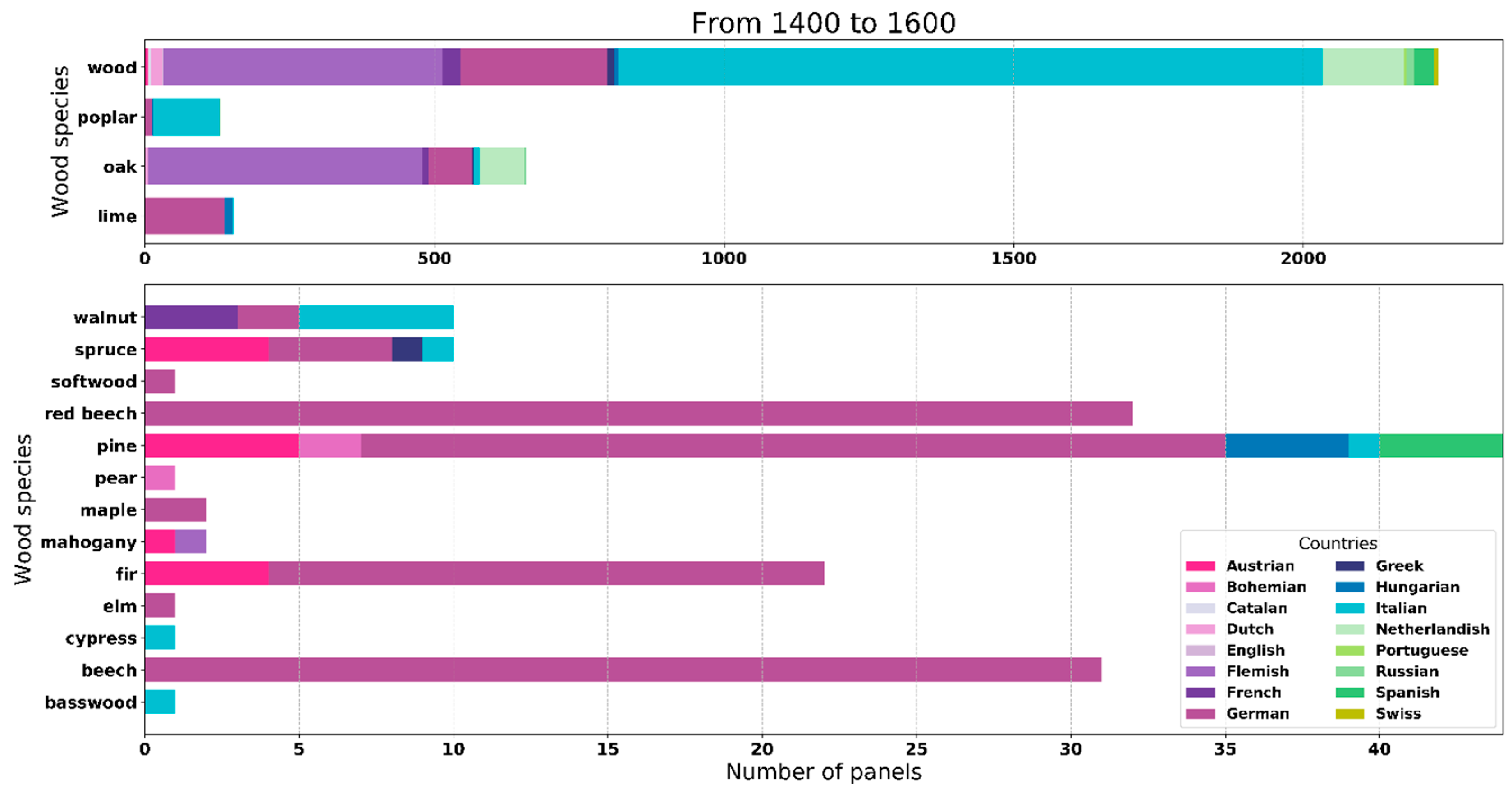
Figure 1 represents wood species used by painting schools during the 15
th and 16
th centuries from all panels available on Web Art Gallery database. The bars represent the number of panels for each wood specie in the focused centuries. The colours represent the place of origin of the panels. Two bar charts were plotted for scale purposes. The upper graph represents the identified species used the most in the 15
th and 16
th centuries with the specie called “wood” which represent the panel with an unidentified specie. The other graph represents the marginal species.
Table 2 and
Table 3 resume the main wood species and the countries of main painting schools of
Figure 1 respectively.
Table 4 shows that we do not know the specie of most of the Italian, German, Netherlandish or French panels but almost half of Flemish panels of this database have identified wood species. This leads to the conclusion that in this period Flemish oak panels are the most popular panels.
The reactions due to RH variations are linked in a part to the wood specie of the object. The fact that a majority of the wooden panels have not had their wood specie identified can make interpretations of images given by the DHSPI more difficult. Knowing this, only the wooden panels whose wood specie are known are kept for further investigations
The set of data base on C2RMF database from 1400 to 1600 contains 662 panels (
Table 5). Italian poplar wood panels are the most common kind of panels with more than 52% of the panels. Almost 92% of poplar panels are Italian and more than 95% of Italian panels are made with poplar. Dutch oak panels are very few, but Flemish oak panels are almost 19% of the panels of the database in this configuration. French painters weren’t always using oak for their panels but apparently most of the Flemish panels gone through the laboratory were made with oak.
Table 6 shows the number of panels by wood specie and country of origin for the C2RMF database with only Louvre panels. The museum had a lot of Italian poplar panels analysed and as previously almost all Italian panels are made with poplar and most of the poplar panels are Italian. Their second popular specie is oak. As the previous set of data, Louvre has a majority of Flemish panels made with oak. From those two sets of data, we can see that oak was most used in Northwest regions of Europe, this not seemed to be the case in French painters who apparently used poplar too.
We resumed Web Art Gallery database in the same way as C2RMF database in
Table 7. It presents 1100 wooden panels painted with identified wood species that were found for these two centuries. French panels here are completely irrelevant, on the contrary German panels are more represented. The comparison was made with the previous results on the C2RMF database. The same conclusion about Flemish panels, that they favour oak as another wood specie for panels can be drawn. From this database, it seems that identified pine panels come from Germany. Netherlandish panels were almost non-existent in the first database but here it is the third more represented painting school, opposing to the Dutch panels.
From these studies, we can conclude that oak and poplar are the main species of hardwood used to make painting panels during the 15th and 16th centuries. The main specie of softwood seems to be pine. The country of origin is important to determine for example the primer coat to put on the wood, or the size of the growth rings of the wood. Italian school applied gesso made with calcium sulphate that is why gesso is commonly applied on poplar. A second kind of pier layer made with calcium carbonate can be found on the North of the Alps. Therefore, it is usual to find this layer on oak. And since pine seems to be mostly from German schools, the same layer as oak seems applied as primer coat.
3.3. Characteristics of selected samples
In order to define entirely the samples, Catherine Lavier, a wood specialist responsible for dendrochronology, wood identification and conservation, working inside the laboratory for more than 20 years [
20], was consulted. The entire definition of those samples goes through the right thickness and the right cut which depend on the wood specie or the origin (growth rings). The wood species presented to her were the one found in the previous section, so the more representative of wooden panels. The aim of this exchange was to define the right cut for each specie and different thicknesses that are representative of wooden panels found in museums.
The wood specialist has explained based on her own experience that poplar and oak panel where indeed famous species used in panels, nevertheless some artists preferred softwood species for their wooden panels. She added that poplar had usually growth rings about 1 cm per year because they came from Italy [
18]. By contrast, oak panels where from North European countries [
18] in that way the growth rings are less than a millimetre per year. Softwoods are more from Germany or Austria so it seems that the growth rings on the pine panels are about 2 or 3mm per year.
The thicknesses of the panels are not standardised, it depends on the type of wood and also on the century when the panel was created [
18]. The thickness of poplar panels is between 3 cm and 4.5 cm. The oak panels were more refined, the resulting thickness is between 0.8 cm and 3 cm. Thicknesses under these values can be found because they are given not taking into account some unfortunate events as thinned operations or two-sided panels cut in half. It means that the panels observed in museums are sometimes thinner because of the changes made on them.
The museums are trying to minimise with a minimum of effort and resources RH and T variations of their entire building since wood varies with RH variations and other materials cannot be harm by a stable environment. That is why some museums have a RH and T control in their rooms. In order to check if the control is working and the variations are not too high, sensors are installed in places of the museums. These sensors record data of RH and T. For the purpose of better understanding the reactions between RH changes and wood movements, use of a museum data of three rooms containing artworks with sensors in order to follow some of the variations is decided.
The collected data allow to establish representative cycles of artworks usual environments. Once these cycles were defined, they were replicated in a climate chamber. The experiments lead to a progression on understanding wood movements depending on its specie, its thickness and the RH and T variations. In this article, results will be discussed comparing the behaviour of two samples under the same variations, with the same wood specie, the same cut but different thickness.
These samples were made with spruce (
Picea abies), with tangential cut. The shrinkage percentage of this specie for radial cut is 3.9%, for tangential cut is 8.2%, and the ration tangential/radial is 2.1 [
17]. Some characteristics of the two samples are shown in
Table 8.
4. Experimental studies and discussions
4.1. Experimental set-up
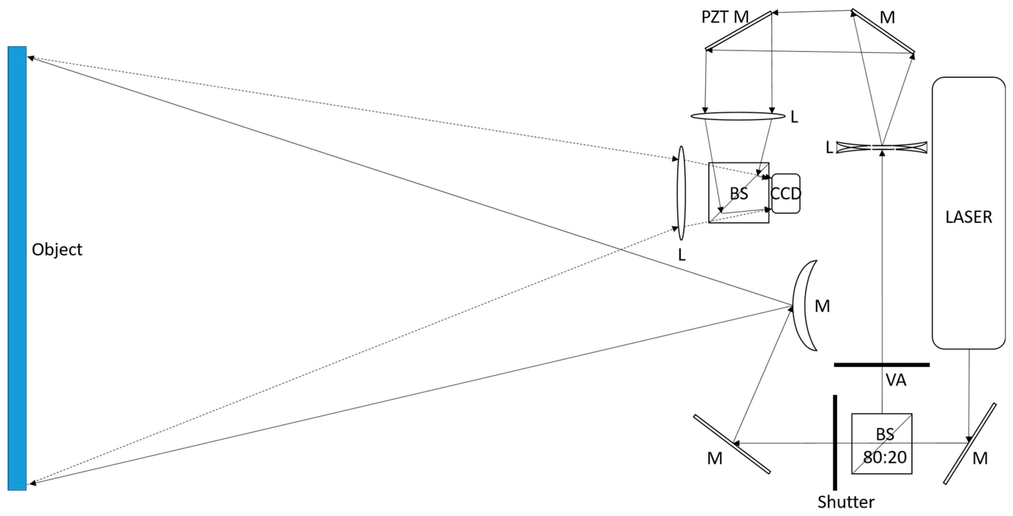
The measurements were done with the DHSPI system. It is a portable system composed on two parts: the optical head and the control unit. The control unit include a central unit, the laser power supply and a RH and T sensor to monitor the room RH and T at each measurement. A portable computer is needed too. The head of the system is mapped in
Figure 2.
The light source is frequency-doubled Nd:YAG laser with a maximal power of 300mW and a coherence length of 30m. It is splitted (Beam splitter: BS) in an object beam with 80% of the laser power illuminating a large part of the object thanks to a convex mirror. The other 20% of the laser beam correspond to the reference beam. The latter goes through a piezoelectric (PZT) mirror. Then, the two beams are recombined by another beam splitter and focused on a CCD sensor with 1600x1200 pixels. This head is closed to avoid any dust, the only moving element is the lens focalising the object image on the camera to allow focusing under optimised conditions. The PZT mirror is precise at some nm in order to capture five images at each time, with a step of . This is a phase-shift measurement.
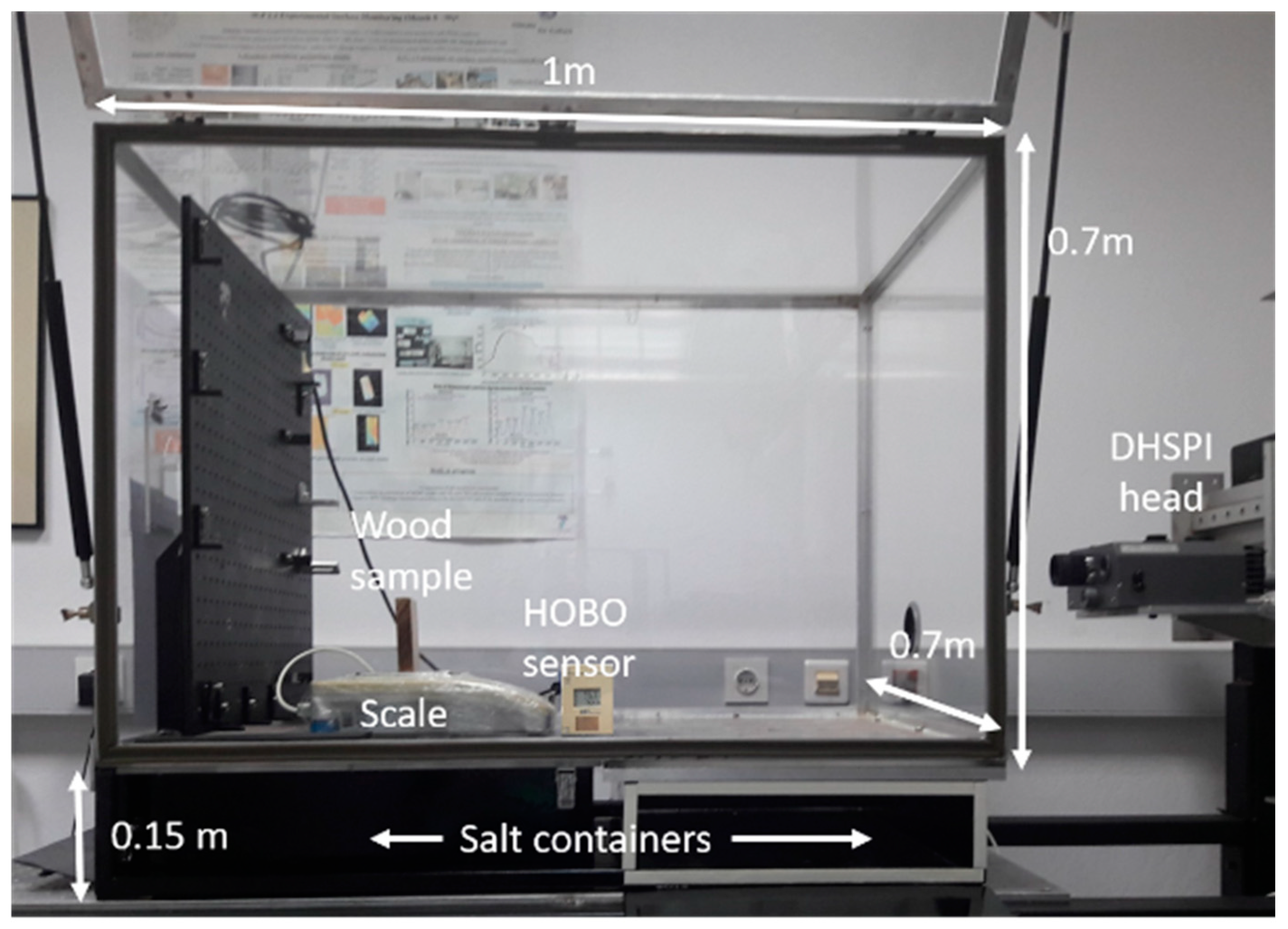
The DHSPI is set to face a sample that is placed on a scale, shown in
Figure 3. The sample and the scale are put in a custom-made climate chamber. It is an airtight construction with two spaces under the main floor which receives the trays of saturated salts solutions to change the RH inside the chamber. To decrease the RH of the chamber, trays of lithium chloride saturated solution were used and to increase the chamber’s RH trays of water vapour are used in the place of salt containers. Those liquids were chosen in order to have relatively slow variations.
The sample is mounted on a digital scale with 0.001 g resolution to measure the weight changes during RH changes. This scale is linked to the DHSPI computer, its acquisition time is customizable and the current acquisition can be followed during the full experimental duration through software developed by the FORTH. An RH/T logger, display, acquire and log the RH and temperature of the chamber. The time between two images acquisitions is adjustable in order to acquire sufficient number of fringes in every image capture.
4.2. Experimental procedure
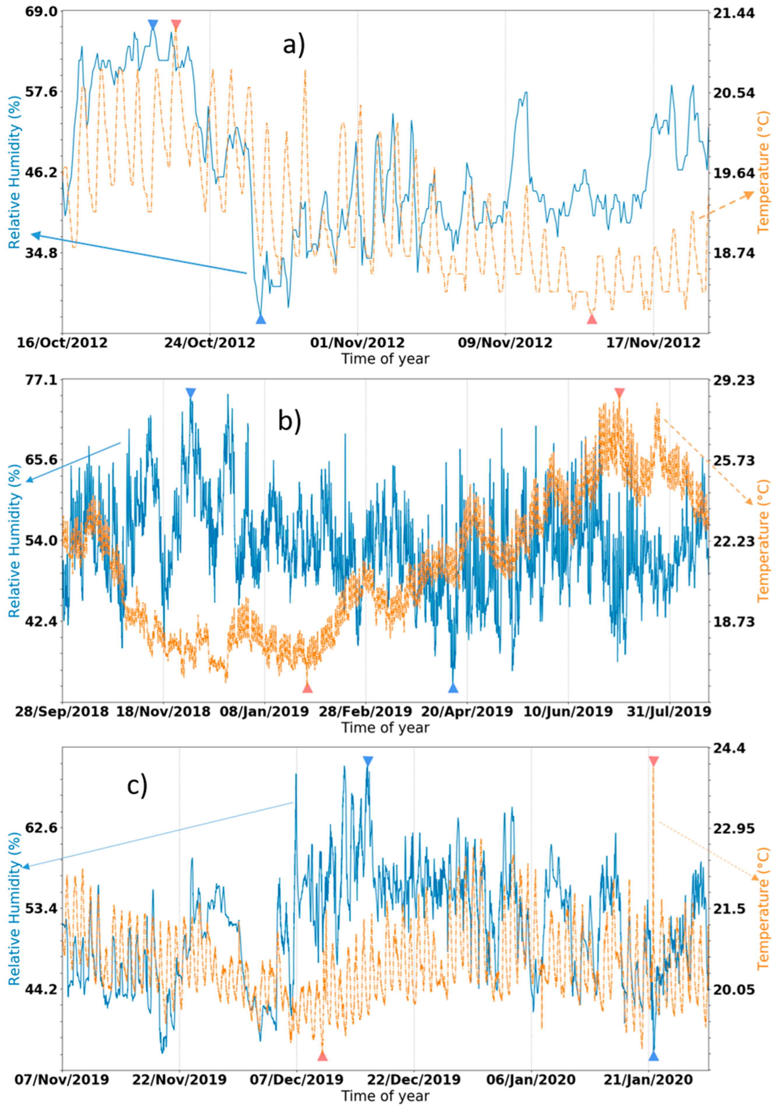
The simulated variations to reproduce on the climate chamber were decided according to a museum RH and T data of three different rooms that are represented in
Figure 4. To stay in a recommended museums condition, the variations of RH must be inferior to 5% per day in order to keep the objects safe.
The first room contains famous artworks, both wooden panels and canvas. The variations in this room can be quite large.
Figure 4a is a plot of T and RH of this room during a month in 2012. The temperature maximum difference is 3.3°C for more than a month. The maximum variation on a day is 2.1°C. The RH value is very low, 25%, at one point and stays low for four days. The worst RH variation during of this period is 21.5%. The set-point temperature is 19°C±1°C, RH is supposed to be greater than 40%.
Figure 4b represents the data of a second room, with Decorative Arts objects. Temperature is programmed to be in winter 19°C±1°C and in summer 25°C±1°C, but RH is not controlled. The temperature is often higher than the setpoint temperature but in winter it can be really below this value, as the minimum is 15.07°C. During summer, it can be higher than 25°C, even reach 28.64°C. Compared to the first room values, here the worst temperature during a day is 3.3°C, this value is the same as the variation happening over a month on the first room. High variations around the year can be seen for RH, but one can suppose these variations are due to the lack of control of T and RH in this room. The worst of the RH variations is 28.6% in 24 hours, a very huge variation for a museum that can endanger the artworks.
Recently a new sensor was installed in a third room containing wooden panels to measure the temperature supposedly at 19°C±2°C. The available data plotted in
Figure 4c are from the installation date to the date when the museum’s conservation Department provided it. The temperature is around more 20.5°C than 19°C. The worst variation is 4.5°C. The RH variations are between 70% and 36%, the worst variation on this range is 27.8%.
With these three graphs we only have the museum’s rooms extremums, 75% is the maximum of all available data coming from the measurements in the second room and 25% is the minimum of all available data coming from the measures in the first room. As the climate chamber is a homemade one, the data can’t be directly loaded in the chamber. That is why the rates per hour of each room have been calculated, in order to find the maximum and minimum rates available in the rooms. These values will determine if the measurements obtained during our experiments are usual in a museum environment, are rarely measured or never measured under normal museum’s conditions.
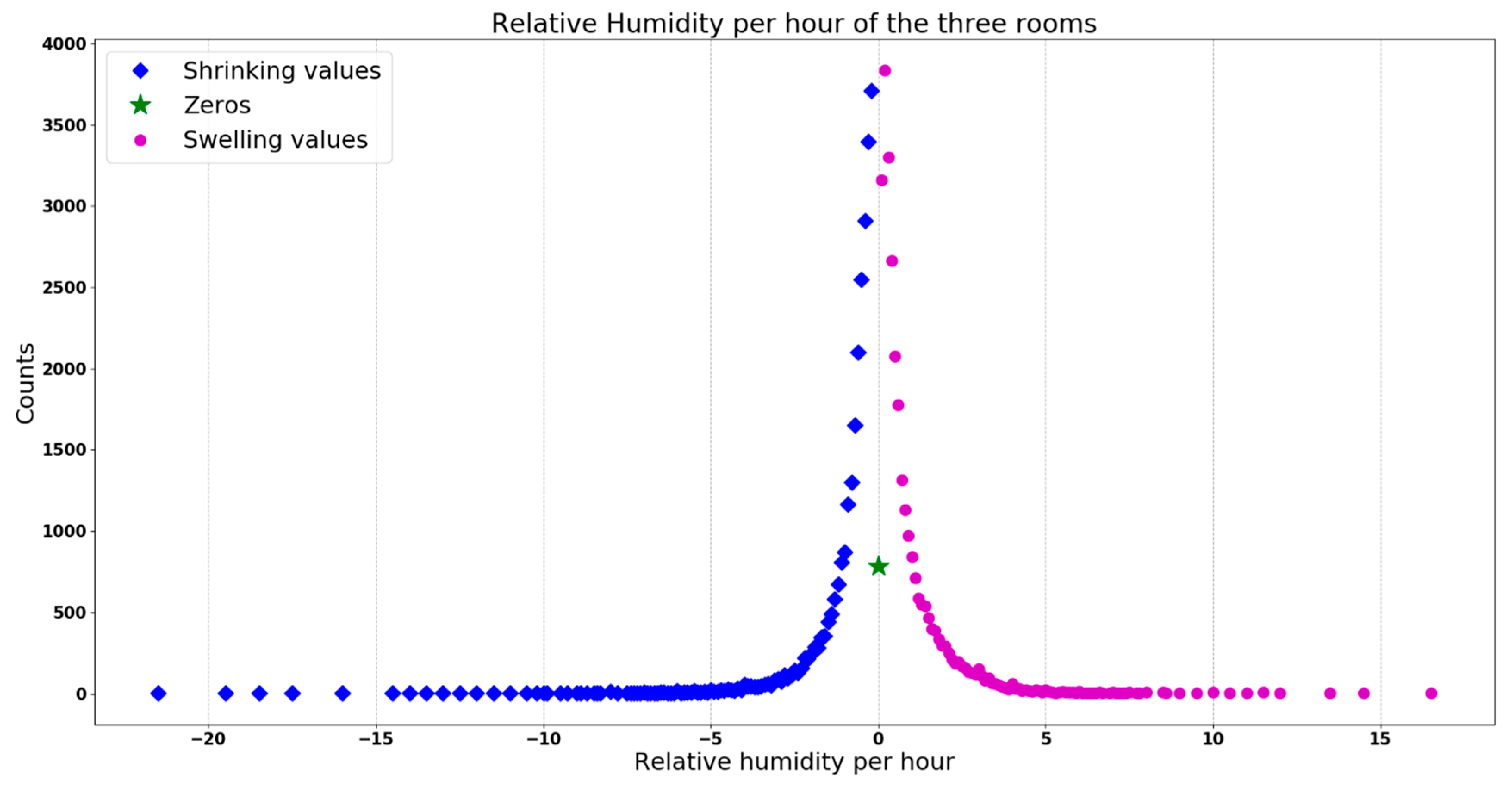
The number of repetition of rates per hour available in the three rooms have been plotted in
Figure 5. It gives the more frequent rates on those rooms. The values plotted here are calculated by taking a value and all that are measured during an hour after it, then by searching for the two extremums in this hour, next by subtracting those two values this gives the RH per hour plotted.
Positive values of RH rates per hour represent RH increasing and are called here swelling value because wood gain water so its moisture content increases during that process. Therefore, the negative values are the decrease of RH and named shrinking values because wood loses water so moisture content decreases. The third type of value is the RH variations that are nulls, therefore it is called zeros.
Figure 5 shows that the maximum RH decrease (minimum shrinking value) is higher than the maximum Rh increase (maximum swelling value). Maximum of the rates per hour have an absolute value of 2%. It means that increase and decrease of RH are quite slow and that despite a lack of control in one room, the museum seems to have found a way to keep RH relatively stable. At least more than 700 relative humidity do not vary during an hour, it means the RH in those cases is stable at least during one hour. By comparing the number of null values and the others, the conclusion is that the museum has more variations of RH, even if they are very low, than stable values.
In order to take into account the rates per hour numbers, the experiments are planned as follows: shrinking from 75% to 25%, taking into account the maximum and the minimum of the three rooms, followed by a swelling until 75%. The shrinking variations are reached by using trays with saturated solution of lithium chloride: when the RH in the climate chamber is equal to 75%, a tray is put in the chamber, a second one is added 3 hours and 30 minutes later. Then 17 hours and 28 minutes later a third tray is added to reach 25%, the minimum found with the museum’s data. As the rate per hour seems to be null, we go to the swelling variations after 1 hour and 40 minutes. The swelling part is achieved by putting different trays of water in the climate chamber. First, a glass round tray with 150 mL of water replaces the trays of lithium chloride, than a larger tray replace this one and the experiment is stopped the next day. These experiments ran for 2 days: one day to decrease the RH is the chamber and almost the other one to increase it. During that time, the temperature is kept around 20.7°C by using the air conditioning in the laboratory.
4.3. Experimental results and discussions
During the experiment, the temperature with room air conditioning on is arranged between 20.57°C and 20.95°C, so it is considered as constant. Hence, the samples variations of surface and mass measured are due to the RH variations only. In regards to the protocol, 25% of RH was never reached. The lowest RH point with this protocol depends on the experimental initial conditions. The initial condition of the chamber for the sample n°51 was a RH stabilised 82% but for the sample n°44, the RH was raised quickly to 75%. This second initial condition allowed the chamber to have a RH at 27%, otherwise it has only been to 29%. Hence, the experiments on n°44 started at 75% RH and the one on n°51 started at 80% RH.
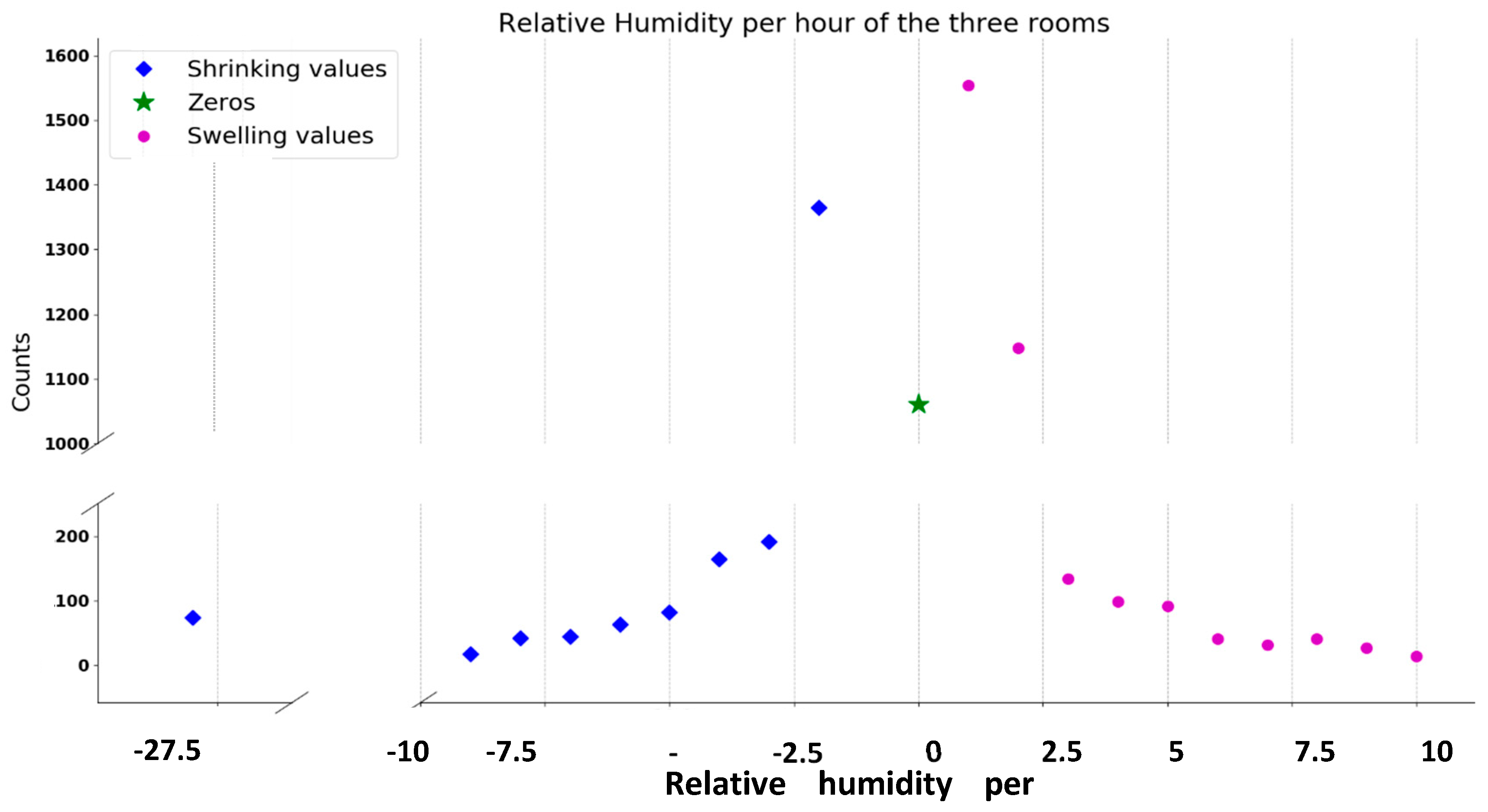
To validate our experiments, the RH rates per hour need to be compared to the data retrieved in the museum’s rooms. The RH rate per hour were calculated as previously and were plotted in
Figure 6. This graph shows that the majority of RH rates per hour obtained during the experiments can be found on museum conditions. In that case, the process used here can be validated.
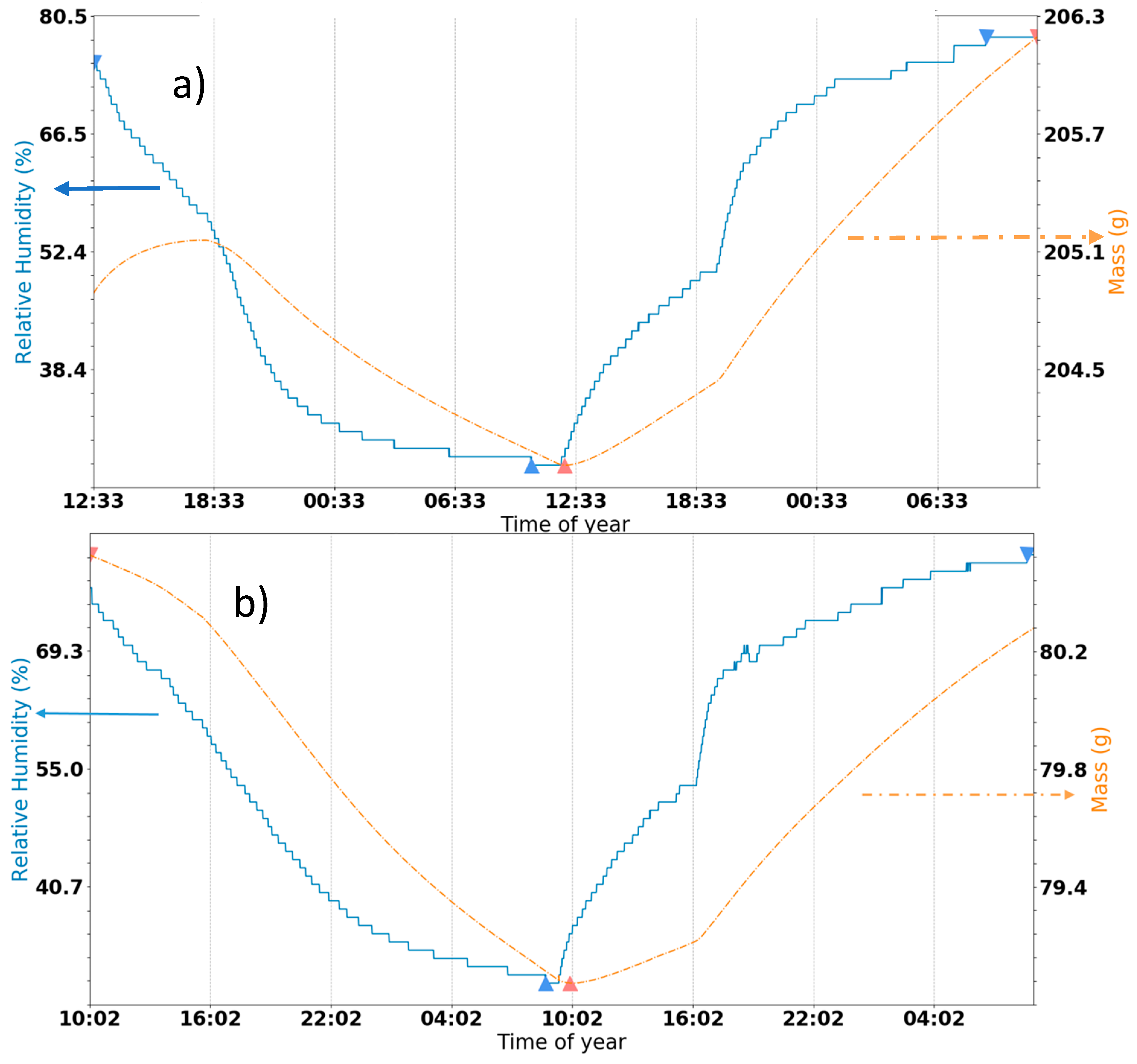
Figure 7 shows the RH of the chamber in percentage versus time with the sample mass in grams versus time of sample n°44 and on n°51. One purpose for the comparison of these two curves is to correlate RH behaviour with the sample mass behaviour. One other aim of this graphs is to define the delay between the mass minimum and the RH minimum, because it has been shown by studies of wooden samples submitted to RH variations [
13,
14,
15] that sample mass variation follows the RH climate chamber variation with a delay written
. To easily show that, triangles have been drawn on the graphs. They show an extremum of the curves, the triangles up are minimums and the ones down are maximums.
Figure 7a represents the RH and mass values versus time of sample n°44, the mass curve does not follow the RH curve in the beginning. This behaviour is explained because the sample was put in the climate chamber right before the experiment start. The room where the sample was stored had a RH value around 44% and the sample was in equilibrium in this environment. The sample did not remain enough time at a stable 75 % of RH in the climate chamber to not increase its moisture content during the beginning of the experiment. After this mass increase, the mass decreases and follow RH variations even if it is with a delay. At the end of the curve, the RH is stable. In spite of that, the mass of the sample is still increasing, so the sample is not in equilibrium with its environment. From this, one can conclude that the sample will not be in equilibrium before 5 hours and 11 minutes, time between the two maximums
Figure 7b represents RH and mass values of versus time sample n°51, the mass curve follows the RH curve during all the experiment. The problem that happened with the sample n°44 in the beginning did not occur because the sample remained enough time in the climate chamber in an environment with stable RH before the experiment start to be in equilibrium with its surrounding environment. The experiment ended before the sample find equilibrium with its surrounding environment.
Since the scale is the same on the two graphs, we can see that the delay between the minimum of the RH curve and the one of the mass curve is longer in the case of sample n°44. For sample n°51,
. For sample n°44,
. Since the only significant difference between the two samples is their thickness, it is clear that the delay depends on the thickness of the wood. Sample n°44 has a thickness of 50mm (
Table 8) and sample n°44 of 19.5mm: the thicker is the wooden object, the longer will be the delay.
Since the mass of an artwork can’t be easily taken if it can be, another method needs to be used to define wood changes during RH variations. In that respect measure of a surface variations of the sample during the experiment were carried out. The purpose is to understand the sample’s surface reactions due to variations of its surrounding RH with the help of the sample mass variations.
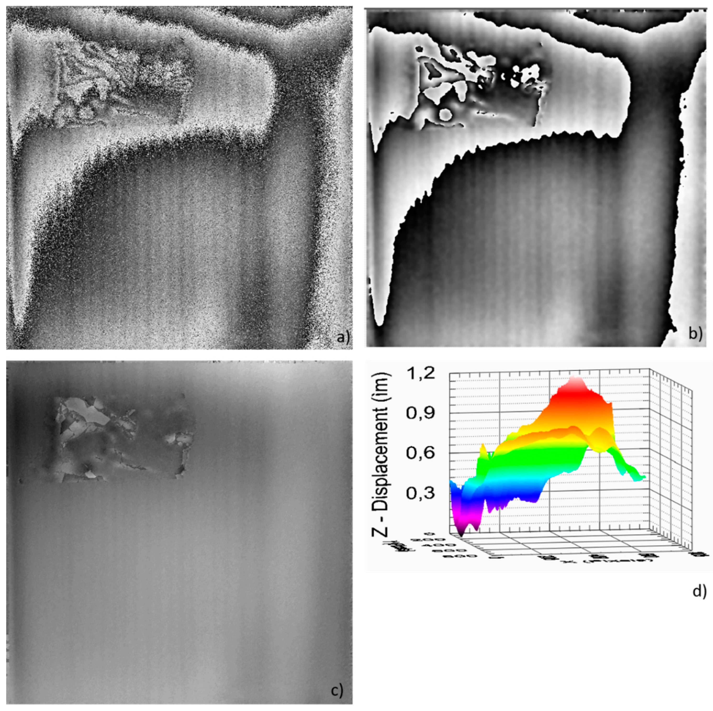
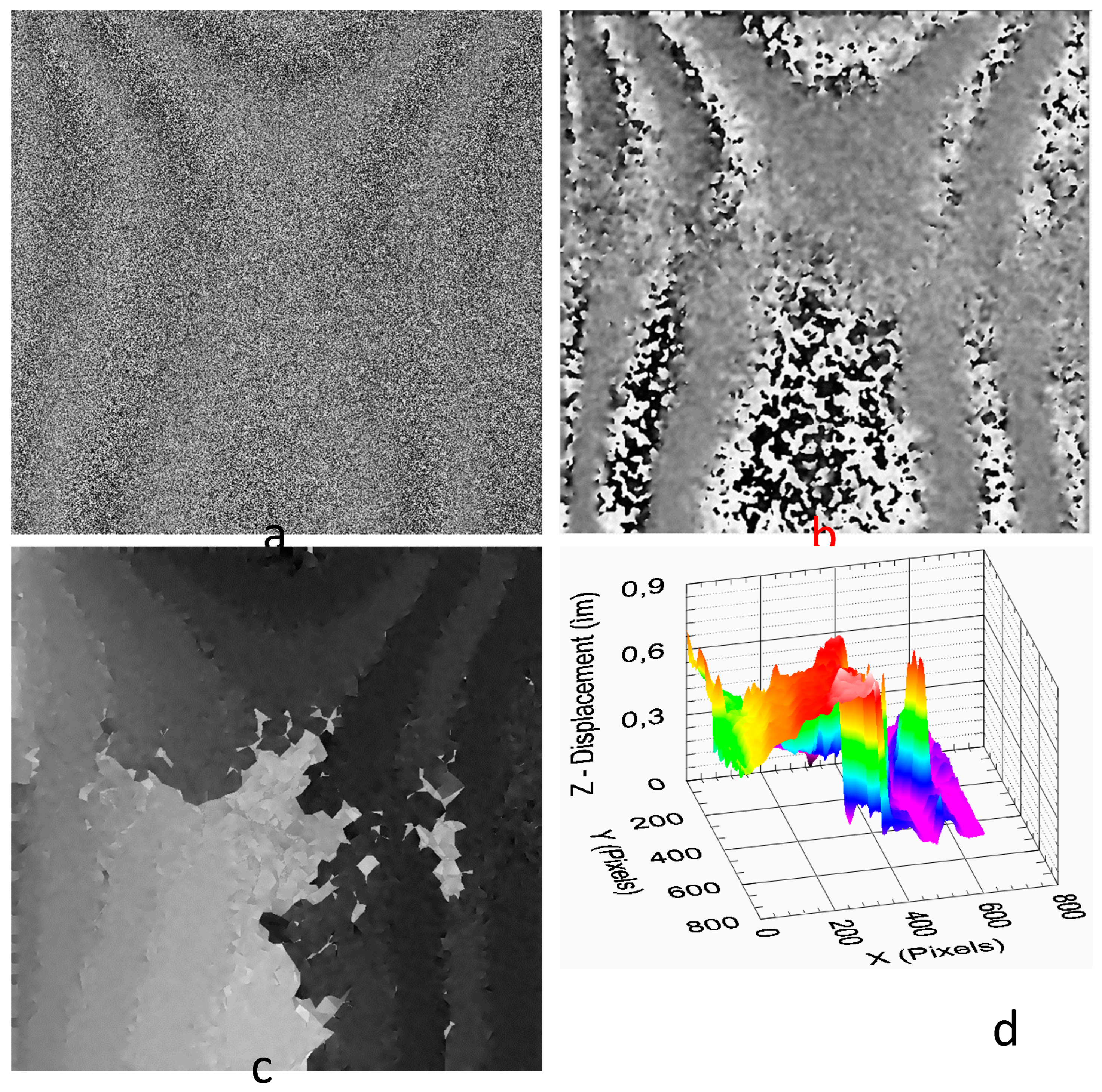
The measurements were made with the DHSPI system. This device acquires a set of five images every five minutes in our experiments. The system recorded these images and displayed the results of their superposition-an interferogram. Examples of those interference patterns are given in
Figure 8a and
Figure 9a. They represent the surface displacement of sample n°44 and sample n°51 respectively. They are the superposition between the surface at 3 hours and 5 minutes and the surface at 3 hours and 10 minutes.
Figure 8b and
Figure 9b are the interferograms after denoising by an optimum process created by FORTH software.
Figure 7c and
Figure 8b are the unwrapped phase of the interferogram based on the denoised pictures.
Figure 7d and
Figure 8d are the 3d representations of the surface of the sample n°44 and the sample n°51, respectively.
Figure 8 shows the surface of sample n°44. The phase maps, wrapped and unwrapped show that the sample n°44 has a default on the upper left at the beginning of the experiment. This default is visible because the image has two different interference patterns. This default is caused by the presence of a sticky paper on this surface and not at all because the wooden sample has a weakness. The 3D map shows that the surface is submitted to a displacement of 1.2 µm in five minutes.
Figure 9 represents the surface of sample n°51. On the interference pattern after processing, one can only see a single interference pattern, so the sample seems to have no defaults at the beginning of this experiment. The unwrapped phase is noisy, because of the noisy interferogram. Since the 3D map comes from this unwrapped image, this is not very reliable but it gives an order of magnitude which gives a displacement of 0.9 µm of the surface in five minutes.
To understand the surface reactions, the denoised images are used to calculate the number of fringes which leads to the surface displacement by
where Δz is the displacement of the surface, λ is the wavelength of the laser (here 532 nm), N is the fringes number of the interference figure.
In order to compare the RH of the climate chamber, the mass of the sample and its surface displacement all those values are divided by
Δt in hour. This gives a RH per hour, a mass per hour that are called here rates per hour and for the surface displacement a new quantity is given: the rate of displacement (RoD) [
15]
where Δz is the displacement of the surface taking place during Δt which is the difference between the acquisitions of two images in hours.
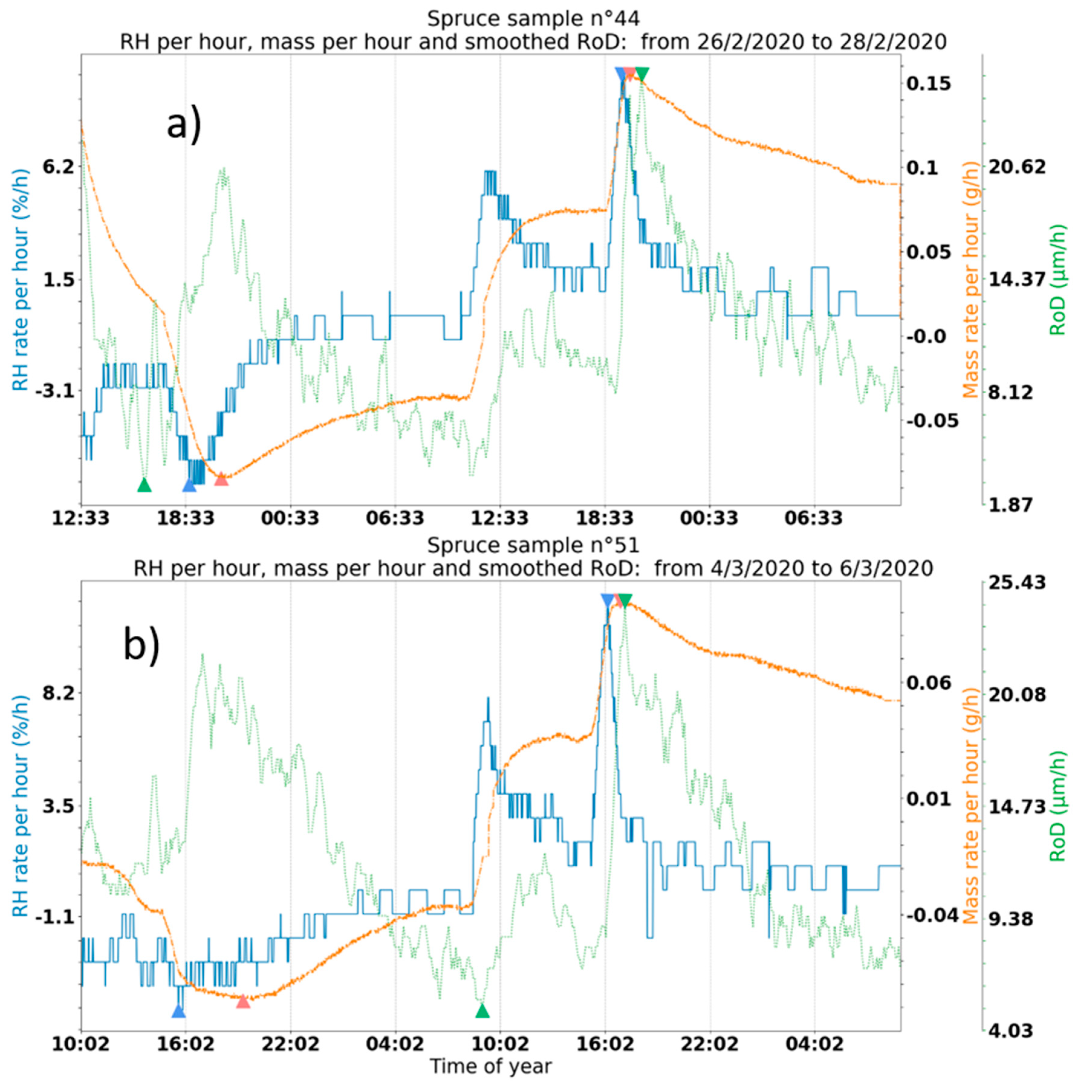
Figure 10 represents the rates per hour of RH versus time, the mass rates per hour versus time and RoD in µm/g versus time of samples n°44 and n°51. The minimums of each curve are shown by triangles with a head up and the maximums with triangles in the down direction. The RoD curves follows the mass rates per hour curves that follows with a delay the RH rates curves. If the variations of RH are fast, the RoD will be higher due to an increasing N, caused by a surface displacement between two images quite large, created by a high moisture variation in the sample. The number of fringes N being always a positive value. It means that when a minimum of mass rate is achieved, a maximum of RoD is reached at the same time, same for a mass rate maximum.
Figure 10a represents the rates per hour of RH and mass versus time, and RoD versus time of the sample n°44. As seen previously on
Figure 7a, the mass curve does not follow the RH curve at the beginning of the experiment. The RoD increases when mass and RH rates values are going further from the zero rates, it decreases when the rates are going nearer to the zeros rate value. The minimum mass rate corresponds to a maximum of ROD. The maximum of RoD is closer to the mass maximum rate than the RH maximum rate. As seen in
Figure 7a, the RH variations are null at the end of the experiments on sample n°44. Despite that, the mass is still variating even if it is less fast. During this part of the experiment, the RoD is still varying. It means that the surface of the sample is moving with a change of mass exclusively. This case does not interest us because the RH in a museum will rarely be stable for so long. On the other end, it shows that the mass changes influence the RoD values, so the surface changes.
Figure 10b represents the rates per hour of RH and mass versus time, and RoD versus time of the sample n°51. The RoD increases when mass and RH rates values are going further from the zero rates, it decreases when the rates are going nearer to the zeros rate value. The maximum mass rate corresponds to the maximum of ROD.
From the observations of the curves, it can be concluded that the mass variations have a higher impact on the surface changes. The scale of RoD of the sample n°51 has a maximum and a minimum higher than the scale of RoD of sample n°44. Since the sample n°51 is thinner than the sample n°44, it means that the displacement of the surface is more important for a thinner wood object.
5. Conclusions
In this study, a design of wooden samples has been realised. This samples represents panels of the 15th and 16th centuries. They also take into account the previous samples used with the DHSPI system in the custom-made climate chamber of the FORTH. The study of two databases of wooden panels shows that a large number of those wooden panels has its wood specie / species not identified by either history of art or scientific method (dendrochronology). The most identified wood of those databases is made of either oak or poplar. More productive places in that period were Flanders using usually oak and Italy preferring poplar. The more common softwood specie was pine and was used in Germany. Oak panels were usually cut into a radial way, contrary to poplar ones which were tangential. Panels are usually thicker if there are made in poplar and thinner if it is oak.
The second step of this study was to determine a cycle of RH variations to reproduce in a climate chamber to observe the surface changes depending on the RH variations. As the study is focused on museum conditions, RH and T data from a museum were used for the cycle determination. From that a process was designed in order to reach the maximum and the minimum values obtained in the museum without exceed the maximum rates per hour of the three rooms.
Regarding to the experiments, the first conclusion is that the initial conditions with the proposed protocol have a real impact on the minimum RH value that can be reached and the mass behaviour. It might be more interesting to stabilise the sample before beginning the experiments, especially to have mass variations that follows all along the experiment the RH variations.
To correlate DHSPI measurements of the surface and RH variations, a direct method was used to measure the samples changes. This method was the use of a scale to measure weight changes of the wooden samples. Mass evolutions follows RH variations with a delay. That delay is related to the sample thickness: it is shorter if the thickness is thinner. The mass rate variations follow also the RH rate variation with a delay. We can conclude that mass gain or losses are due to moisture variations in the panel, leading to its deformation. This process follows RH changes and it is visible by the number of fringes given by a DHSPI interferograms which are related to the surface deformation of the panel. This deformation is measured every 5 minutes and the interferograms represents the surface deformation during this time difference. Because of the delay response of the material system, the study of the fringes number seems not to be accurate enough to monitor these mass variations when the RH variations are sudden.
Author Contributions
Conceptualization, J.A., V.D. and V. T; methodology, V.T. and V.D.; software, J.A.; validation, J.A., M.A., V.D. and V.T.; formal analysis, J.A. and V.T.; investigation, J.A. and M.A.; resources, J.A., X.B. N.W. and V.D.; data curation, J.A. And M.A.; writing—original draft preparation, J.A. and X.B.; writing—review and editing, all authors.; visualization, J.A., X.B., N.W., V.T. and V.D.; supervision, N.W., V.T. and V.D.; project administration, V.D.; funding acquisition, V.D and N.W. All authors have read and agreed to the published version of the manuscript.
Funding
This work was supported by the Paris Seine Graduate School Humanities, Creation, Heritage, Investissement d’Avenir ANR-17-EURE-0021 – Foundation for Cultural Heritage Science. The experimental work was conducted at Holography laboratory at Institute of Electronic Structure and Laser/Foundation for Research and Technology-Hellas (IESL/FORTH) of the Ultraviolet Laser Facility supported in part by the European Union's Horizon 2020 research and innovation programme LASERLAB-EUROPE (Grant Agreement No. 654148 or 871124)
Data Availability Statement
The data that support the findings of this study are available from the corresponding author upon reasonable request.
Conflicts of Interest
The authors declare no conflict of interest.
References
- Bertolin, C., L. de Ferri, and F. Berto, Calibration Method for Monitoring Hygro-Mechanical Reactions of Pine and Oak Wood by Acoustic Emission Nondestructive Testing. Materials (Basel), 2020. 13(17): p. 3775. [CrossRef]
- Anaf, W., et al., Real-Time Wood Behaviour: The Use of Strain Gauges for Preventive Conservation Applications. Sensors, 2020. 20(1): p. 305. [CrossRef]
- Tornari, V. and K. Papadaki. Continuous wave and pulse holographic interferometry used for monitoring environmental effects on materials used in artefacts. in Proc. of the 1st International Congress on Science and Technology for the safeguard of Cultural Heritage in the Mediterranean Basin, Catania-Siracusa. 1995.
- Tornari, V., Holographic Interferometry: A diagnostic tool for the conservation of artworks. V&A Newsletter Conservation Magazine, Victoria & Albert museum, 1995.
- Brewer, A. and C. Forno, Moiré fringe analysis of cradled panel paintings. Studies in Conservation, 1997. 42(4): p. 211-230.
- Ashley-Smith, J., N. Umney, and D. Ford, Let's be honest — realistic environmental parameters for loaned objects. Studies in Conservation, 1994. 39(sup2): p. 28-31.
- Falciai, R., et al. The monitoring of painted wood panels by fibre Bragg grating sensors. in Conservation science 2002: papers from the conference held in Edinburgh, Scotland 22-24 May 2002. 2003. 24 May.
- Bratasz, Ł. and R. Kozłowski, Laser Sensors for Continuous In-Situ Monitoring of the Dimensional Response of Wooden Objects. Studies in Conservation, 2005. 50(4): p. 307-315. [CrossRef]
- Bratasz, Ł., et al., Impact of Indoor Heating on Painted Wood - Monitoring the Altarpiece in the Church of Santa Maria Maddalena in Rocca Pietore, Italy. Studies in Conservation, 2007. 52(3): p. 199-210. [CrossRef]
- Oh, G.-H., et al., In-situ monitoring of moisture diffusion process for wood with terahertz time-domain spectroscopy. Optics and Lasers in Engineering, 2020. 128: p. 106036. [CrossRef]
- Jakieła, S., Ł. Bratasz, and R. Kozłowski, Acoustic Emission for Tracing the Evolution of Damage in Wooden Objects. Studies in Conservation, 2007. 52(2): p. 101-109. [CrossRef]
- Tornari, V., Laser interference-based techniques and applications in structural inspection of works of art. Analytical and Bioanalytical Chemistry, 2007. 387(3): p. 761-780. [CrossRef]
- Camuffo, D., Microclimate for Cultural Heritage: Measurement , Risk Assessment, Conservation, Restoration, and Maintenance of Indoor and Outdoor Monuments. Elsevier, 2019.
- Tornari, V., et al., Fully-non-contact masking-based holography inspection on dimensionally responsive artwork materials. Sensors, 2008. 8(12): p. 8401-8422. [CrossRef]
- Tornari, V., et al., Preventive deformation measurements on cultural heritage materials based on non-contact surface response of model samples. Studies in conservation, 2015. 60(sup1): p. S143-S158. [CrossRef]
- Tornari, V., et al., Impact of Relative Humidity on Wood Sample: A Climate Chamber Experimental Simulation Monitored by Digital Holographic Speckle Pattern Interferometry. Journal of Imaging, 2019. 5(7): p. 65. [CrossRef]
- Rzecki, K., et al., Application of computational intelligence methods for the automated identification of paper-ink samples based on LIBS. Sensors, 2018. 18(11): p. 3670. [CrossRef]
- Hoadley, R.B., et al., The Structural Conservation of Panel Paintings: Proceedings. Part 1: Wood Science and Technology. null. Vol. 1. 1998. 127.
- Hoadley, R.B., Understanding Wood: A Craftsman’s Guide to Wood Technology. Vol. null. 2000. null.
- Lavier, C., T. Borel, and D. Vigears, Tracéologie appliquée aux objets et œuvres d’art en bois des musées de France: premiers exemples d’adaptations, de développements techniques et de résultats au sein du C2RMF. Technè, 2009. 29: p. 15-18.
Figure 1.
Wood species used by painting schools, Web Art Gallery database.
Figure 1.
Wood species used by painting schools, Web Art Gallery database.
Figure 2.
Schematic of DHSPI head. M: mirror; PZT M: piezoelectric mirror; BS: beam splitter; L: lens; VA: variable attenuator.
Figure 2.
Schematic of DHSPI head. M: mirror; PZT M: piezoelectric mirror; BS: beam splitter; L: lens; VA: variable attenuator.
Figure 3.
Opened homemade climate chamber for DHSPI monitoring.
Figure 3.
Opened homemade climate chamber for DHSPI monitoring.
Figure 4.
a) Relative humidity vs time and temperature vs time between October 16th 2012 and November 11th 2012 for the first room of the museum. b) Relative humidity vs time and temperature vs time between September 28th 2018 and August 20th 2019 for the second room of the museum. c) Relative humidity vs time and temperature vs time between November 7th 2019 and January 28th 2020 for the third room of the museum. Triangles down represents maximums and tringles up represents minimums.
Figure 5.
RH rates per hour available for museum’s rooms data.
Figure 5.
RH rates per hour available for museum’s rooms data.
Figure 6.
RH rates per hour measured during experiments on sample n°44 and sample n°51.
Figure 6.
RH rates per hour measured during experiments on sample n°44 and sample n°51.
Figure 7.
a) represents the values for sample n°44, the mass does not follow the RH in the beginning because the sample did not remain enough time in the climate chamber in an environment with stable RH before the start of the experiment to be in equilibrium. The mass is going up before going down since RH was increasing before the start of the experiment. The experiment ended before the sample find equilibrium with its surrounding environment. Triangles down represents maximums and tringles up represents minimums.
Figure 8.
Sample n°44 interference figure during shrink process. a) Row data b) after denoising. c) Unwrapped phase of the denoised image d) 3d map of the displacement of the sample n°44 surface.
Figure 8.
Sample n°44 interference figure during shrink process. a) Row data b) after denoising. c) Unwrapped phase of the denoised image d) 3d map of the displacement of the sample n°44 surface.
Figure 9.
Sample n°51 interference figure during shrink process. a) Row data b) after processing c) Unwrapped phase of the denoised image d) 3d map of the displacement of the sample n°51 surface.
Figure 9.
Sample n°51 interference figure during shrink process. a) Row data b) after processing c) Unwrapped phase of the denoised image d) 3d map of the displacement of the sample n°51 surface.
Figure 10.
a) Sample n°44 rates per hour of RH (%/h) vs time, mass rate per hour (g/h) vs time and RoD vs time. b) Sample n°51 rates per hour of RH (%/h) vs time, mass rates per hour (g/h) vs time and RoD vs time. Triangles down represents maximums and tringles up represents minimums.
Figure 10.
a) Sample n°44 rates per hour of RH (%/h) vs time, mass rate per hour (g/h) vs time and RoD vs time. b) Sample n°51 rates per hour of RH (%/h) vs time, mass rates per hour (g/h) vs time and RoD vs time. Triangles down represents maximums and tringles up represents minimums.
Table 1.
Techniques used in conservation of wood for cultural heritage.[
11,
12,
13].
Table 1.
Techniques used in conservation of wood for cultural heritage.[
11,
12,
13].
| Technique |
Apparition date |
Sensitivity |
| Moiré fringes |
1954 |
µm accurancy |
| Fibre Bragg grating |
1978 |
Less than 100 nm |
| Triangulation displacement sensor |
1980s |
µm accurancy |
| THz domain |
1980s |
Less than 100 ps |
| Wood specie |
Number of artworks |
Percentage |
| Wood |
2226 |
66.98% |
| Poplar |
131 |
3.93% |
| Oak |
658 |
19.74% |
| Pine |
44 |
1.32% |
Table 3.
Main painting schools of
Figure 1.
Table 3.
Main painting schools of
Figure 1.
| Painting school |
Number of artworks |
Percentage |
| Italian |
1351 |
40.52% |
| Flemish |
957 |
28.7% |
| French |
43 |
1.29% |
| German |
597 |
17.91% |
| Netherlandish |
219 |
6.57% |
Table 4.
Main wood species with their painting school from
Figure 1.
Table 4.
Main wood species with their painting school from
Figure 1.
| Wood species |
School |
Number of artworks |
Percentage |
| Wood panels |
Italian schools |
1215 |
36.44% of entire data - 89.93% of Italian - 54.41% of wood |
| Flemish schools |
482 |
14.46% of entire data - 50.37% of Flemish - 21.59% of wood |
| French schools |
31 |
0.93% of entire data - 72.09% of French - 1.39% of wood |
| German schools |
253 |
7.59% of entire data - 42.38% of German - 11.33% of wood |
| Netherlandish schools |
141 |
4.23% of entire data - 64.38% of Netherlandish - 6.31% of wood |
| Poplar panels |
Italian schools |
114 |
3.42% of entire data - 8.44% of Italian - 87.02% of poplar |
| Oak panels |
Flemish schools |
474 |
14.22% of entire data - 49.53% of Flemish - 72.04% of oak |
| French schools |
9 |
0.27% of entire data - 20.93% of French - 1.37% of oak |
| German schools |
76 |
2.28% of entire data - 12.73% of German - 11.55% of oak |
| Netherlandish schools |
78 |
2.34% of entire data - 35.62% of Netherlandish - 11.85% of oak |
| Pine panels |
German schools |
28 |
0.84% of entire data - 4.69% of German - 63.64% of pine |
Table 5.
Main wood species with their painting school from C2RMF database with only known species containing 662 panels.
Table 5.
Main wood species with their painting school from C2RMF database with only known species containing 662 panels.
| |
Oak panels: 35.65% |
Poplar panels: 54.68% |
| Dutch panels: 2.87% |
2.42% of entire data
84.21% of Dutch panels
6.78% of oak panels |
0.15% of entire data
5.26% of Dutch panels
0.28% of poplar panels |
| Flemish panels: 19.03% |
18.58% of entire data
97.62% of Flemish panels
52.12% of oak panels |
0.15% of entire data
0.79% of Flemish panels
0.28% of poplar panels |
| French panels: 13.9% |
9.97% of entire data
71.74% of French panels
27.97% of oak panels |
0.91% of entire data
6.52% of French panels
1.66% of poplar panels |
| German panels: 3.17% |
2.42% of entire data
76.19% of German panels
6.78% of oak panels |
0.3% of entire data
9.52% of German panels
0.55% of poplar panels |
| Italian panels: 57.1% |
0.91% of entire data
1.59% of Italian panels
2.54% of oak panels |
52.42% of entire data
91.8% of Italian panels
95.86% of poplar panels |
Table 6.
Main wood species with their painting school from C2RMF database, Louvre data with only known species containing 400 panels.
Table 6.
Main wood species with their painting school from C2RMF database, Louvre data with only known species containing 400 panels.
| |
Oak panels: 27.5% |
Poplar panels: 61.75% |
| Dutch panels: 3% |
2.5% of entire data
83.33% of Dutch panels
9.09% of oak panels |
0.5% of entire data
16.67% of Dutch panels
0.81% of poplar panels |
| Flemish panels: 16.25% |
15.75% of entire data
96.92% of Flemish panels
57.27% of oak panels |
0.5% of entire data
3.08% of Flemish panels
0.81% of poplar panels |
| French panels: 7% |
4.25% of entire data
60.71% of French panels
15.45% of oak panels |
0.75% of entire data
10.71% of French panels
1.21% of poplar panels |
| German panels: 6.25% |
3.5% of entire data
56.0% of German panels
12.73% of oak panels |
|
| Italian panels: 64.25% |
0.5% of entire data
0.78% of Italian panels
1.82% of oak panels |
60.0% of entire data
93.39% of Italian panels
97.17% of poplar panels |
Table 7.
Main wood species with their painting school from Web Art Gallery database with only known species containing 1100 panels.
Table 7.
Main wood species with their painting school from Web Art Gallery database with only known species containing 1100 panels.
| |
Oak panels: 59.82% |
Pine panels: 4% |
Poplar panels: 11;91% |
| Flemish panels: 43.18% |
43.09% of entire data
99.79% of Flemish
72.04% of oak panels |
|
|
| French panels: 1.09% |
0.82% of entire data
75.0% of French
1.37% of oak panels |
|
|
| German panels: 31.18% |
6.91% of entire data
22.16% of German
11.55% of oak panels |
2.55% of entire data
8.16% of German
63.64% of pine |
1.18% of entire data
3.79% of German
9.92% of poplar |
| Italian panels: 12.36% |
1.0% of entire data
8.09% of Italian panels
1.67% of oak panels |
0.09% of entire data
0.74% of Italian
2.27% of pine |
10.36% of entire data
83.82% of Italian
87.02% of poplar |
| Netherlandish panels: 7.09% |
7.09% of entire data
100.0% of Netherlandish
11.85% of oak panels |
|
|
Table 8.
Samples characteristics.
Table 8.
Samples characteristics.
| Sample number |
Wood |
Length (mm) |
Width (mm) |
Thickness (mm) |
Growth rings |
Specific gravity |
| 44 |
Spruce |
100 |
100 |
50 |
39 |
0.41 |
| 51 |
Spruce |
100.5 |
99.7 |
19.5 |
22 |
0.4 |
|
Disclaimer/Publisher’s Note: The statements, opinions and data contained in all publications are solely those of the individual author(s) and contributor(s) and not of MDPI and/or the editor(s). MDPI and/or the editor(s) disclaim responsibility for any injury to people or property resulting from any ideas, methods, instructions or products referred to in the content. |
© 2023 by the authors. Licensee MDPI, Basel, Switzerland. This article is an open access article distributed under the terms and conditions of the Creative Commons Attribution (CC BY) license (http://creativecommons.org/licenses/by/4.0/).
