1. Introduction
The critical role of the ocean in the earth climate system is well known and documented as the ocean is the largest carbon sink and heat reservoir absorbing over 93% of heat generated since the industrial revolution (IPCC,201). However, evidence in the scientific literature affirmed that the last few decades has witnessed significant increase in the heat storage capacity of the ocean with deleterious impact on key components of the earth-atmosphere system (Wijffels et al., 2016). The observed Ocean warming manifestation includes increase in average sea surface temperature, changes in ocean circulation, stratification, heat transport, ocean biogeochemistry and marine heat waves with concomitant effect on regional and global climate variability and human societies. It’s on record that average global SST of the ocean have significant warming tend of ~0.13°C per decade since the beginning of the 20th Century with SST of the last there decades considered the warmest since the commencement of modern instrumental records (Robers, 2016) with global warming implicated in the observed warming.
Several studies have been conducted over the years to examine global sea surface temperature distribution and their influence on climate extremes over the West African region. The above assertion is hinged on the fact that the amount of near surface moisture for convective rainfall is sensitive to sea surface temperature anomaly through the Clausius-Clapeyron relationship (Dabo and Takahashi,2017) Another mechanism where SST influence is evident is in the tropical Atlantic ocean is through the interaction with the wind field in which the weakness of the trade winds over the equator forces the Inter tropical Convergence Zone to migrate northwards thereby strengthening southerly trade winds. This interaction ultimately leads to upwelling, vertical missing and evaporation into the atmosphere and eventually leads to a phenomenon called cold tongue which develops in May, June, July persisting till September. It is this seasonal SST anomaly that exercise significant control on rainfall pattern over West African Climate (Lubbecke, et al, 2015).
Consequently, modelling studies by Rowell et,al 1992 and Palmer et al, 1992 corroborates the above analogy on the influence of ocean forcing on rainfall variability in Sub-Saharan Africa. Similar studies have also focused on the impact of localized SST anomalies over the coast of Guinea and the eastern Atlantic Ocean (Newell and Kidson, 1984). Bah studies in 1987 was more emphatic as it revealed that reduction in rainfall in the Sahel during winter corresponded well with warm SST anomaly over the precipitation at the Guinea coast, the global SST variability merely slightly moderate its effects.
Adeniye 2017 in his study assessed the impacts of warming/cooling of the Atlantic sea surface temperature (SST) on the climate of West Africa using Version 4.4 of Regional Climate Model (RegCM4.4A.) The study outcome revealed that 1–2 K cooling and warming of the Atlantic SST will result in tripole temperature and precipitation change structure over West Africa. to an anomalous dipole of precipitation resulting in opposite signs over the Sahel and the Gulf of Guinea
Given the scale and vulnerability of West Africa described as the one of the most populated regions of the world to extreme climate events and climate change manifesting in increased frequency of floods, drought with devastating impact on livelihoods and attainment of the sustainable development goals. The vulnerability is driven mainly by a range of factors that include weak adaptive capacity, dependence on productive resources that are climate sensitive, Africa’s geographical location in the lower latitudes and widespread poverty climate change is also disrupting the hydrological cycle, putting a strain on water resources, population displacement and food insecurity (UNFCCC,2021). This has led the scientific community on the need to mobilize additional resources to mitigate projected impact of climate change on critical sectors of the economy in the sub-region and to build resilience. This is against the backdrop that a warmer climate holds more moisture implying increased frequency of rainfall events. conversely, rising temperature accelerates evaporation and can intensify droughts episodes (Seager et al. 2012,).
The Fourth Assessment Report of Intergovernmental Panel on Climate Change (IPCC) (AR4) projected warming of 0.5–2.5 K over the Atlantic Ocean for the twenty-first century (Christensen et al. 2007) based on all Special Report on Emissions Scenarios (SRES) while the Fifth Assessment report of the IPCC also projected temperature change of 0.2–2.3 K over West Africa (Christensen et al. 2013) based on all the representative concentration pathways (RCPs). In the same vein, the Sixth Assessment report (AR6) of the IPCC 2022 affirmed that the global mean SST has increased since the beginning of the 2oth century by 0.88oC with significant warming projected in the coming decades.
The increase in SST has been reported to be driven by climate change on an oceanic scale, such as the Atlantic equatorial mode and El Niño-Southern Oscillation (ENSO) (Burls et, al, 2012 and Breugeon, 2006). Thus, the understanding of future climate change effects on SST variability and warming in the Gulf of Guinea has become pertinent to investigate. The General Circulation Model (GCMs) outputs of the Coupled Model Intercomparison Project (CMIP) are an essential dataset for forecasting future climate trends. The main difference between the previous CMIP5 models and the current CMIP6 output is based on the set of future scenarios used to project climate evolution. The CMIP6 model was designed to bridge and improve the restrictions identified in the CMIP5 models with a focus on identifying systematic errors in simulations and improving the representation of land use changes on climate (IPCC report). Several new scenarios used by CMIP6 called Shared Socioeconomic Pathways (SSPs), which are in combination with previous CMIP5 scenarios of climate radiative forcing called Radiative Concentration Pathways (RCPs). The GCMs of Coupled Model Intercomparison Project 6 (CMIP6) are the most advanced tools currently available for climate studies and stronger than previous projects. Besides, the GCMs of Coupled Model Intercomparison Project 6 (CMIP6) are also the most advanced tools currently available for climate studies and for simulating past and future extreme climate events given the scale of anthropogenic induced global warming. (Ahmed et al. 2019; Jose and Dwarakish 2020; Sonali and Kumar 2020).
However, GCM simulations cannot be directly used for climate impact studies because of their inability to give reliable information at a local scale (Chokkavarapu and Mandla 2019). Furthermore, GCM outputs are often coarse in the temporal and spatial dimensions, resulting in systematic biases (Ayubi, et al, 2021). Hence, it is critical to validate the skills of these models before use for any climate projection and impact studies. Therefore, downscaling model outputs has necessary so as to improve the model resolution to match the resolution at a local scale. Downscaling essentially is the process whereby spatial data is represented with lower spacing and with smaller temporal intervals (Liz, et al,2022).
Dynamical downscaling and statistical downscaling have emerged as some of the best methods widely used for post-processing GCMs are dynamical downscaling and statistical downscaling. The statistical approach has advantages over dynamical downscaling as it is a lot less resource intensive ( Trasher et al,2012), Additionally, The pros and cons of both approaches is that while Statistical approaches are based on the distribution and relationship between the observed and projected data for the historical period , dynamical downscaling on the other hand is based on regional climate model forced with the boundary conditions from the coarse resolution global circulation model (White and Toumi (2013). In view of the gap identified in the literature on the use of GCM CMIP6 models in simulating historical and future SST of the gulf of the Guinea, it has become critical to examine the skills of CMIP6 models in simulating sea surface temperature over the gulf of Guinea.
The objectives of the study therefore is to evaluate the performance of 8 GCM-CMIP6 models in simulating the historical sea surface temperatures of the Gulf of Guinea from (1970–2014). secondly bias corrected CMIP6 outputs to simulate future SST projection (2015-20100) and finally used statistical techniques to quantitatively validate the performance of the models.
2. Materials and Methods
Projections from the General Circulation Models (GCMs) play a vital role in understanding the future changes in climate. However, spatial resolution at which GCMs are run is often too coarse to get reliable projections at the regional and local scale (Christensen et al., 2008).
The bias-corrected dataset was developed using Empirical Quantile Mapping (EQM) for the historic (1940–2014) and projected (2015–2100) climate for the SSP5-8.5 scenarios using output from 8 General Circulation Models (GCMs) from Coupled Model Intercomparison Project-6 (CMIP6). The bias-corrected dataset was evaluated against the observations for monthly and annual sea surface temperatures (SST) over the Gulf of Guinea as shown in
Table 1 below
The observed monthly gridded SST for Gulf of Guinea for the 1940 –2014 period was obtained from the ERA5 Copernicus data at 0.25° X 0.25° spatial resolution.
The mean monthly SST from 8 CMIP6-GCMs were obtained from
https://esgf-node.llnl.gov/search/cmip6/ . The SST variable was available for both the historical and scenarios under the 8 CMIP6-GCMs used in the study. The spatial resolution of the CMIP6 projection varies from 0.7° (EC-Earth3) to more than 2° (MCM-UA-1-0 (USA). All the three variables were selected for the historical (1940–2014) and ssp585 (2015–2100) scenarios under
r1i1p1f1 initial condition at monthly time scale (Eyring
et al., 2016). The scenarios used in the CMIP6 combine Shared Socioeconomic Pathways (SSP) and target radiative forcing levels at the end of the 21st century. On the other hand, SSP585 is based on the emission scenario considering SSP-5 and radiative forcing of 8.5 Watt/m2 at the end of the 21st century (Gidden
et al., 2019)..
2.1. The Study Area
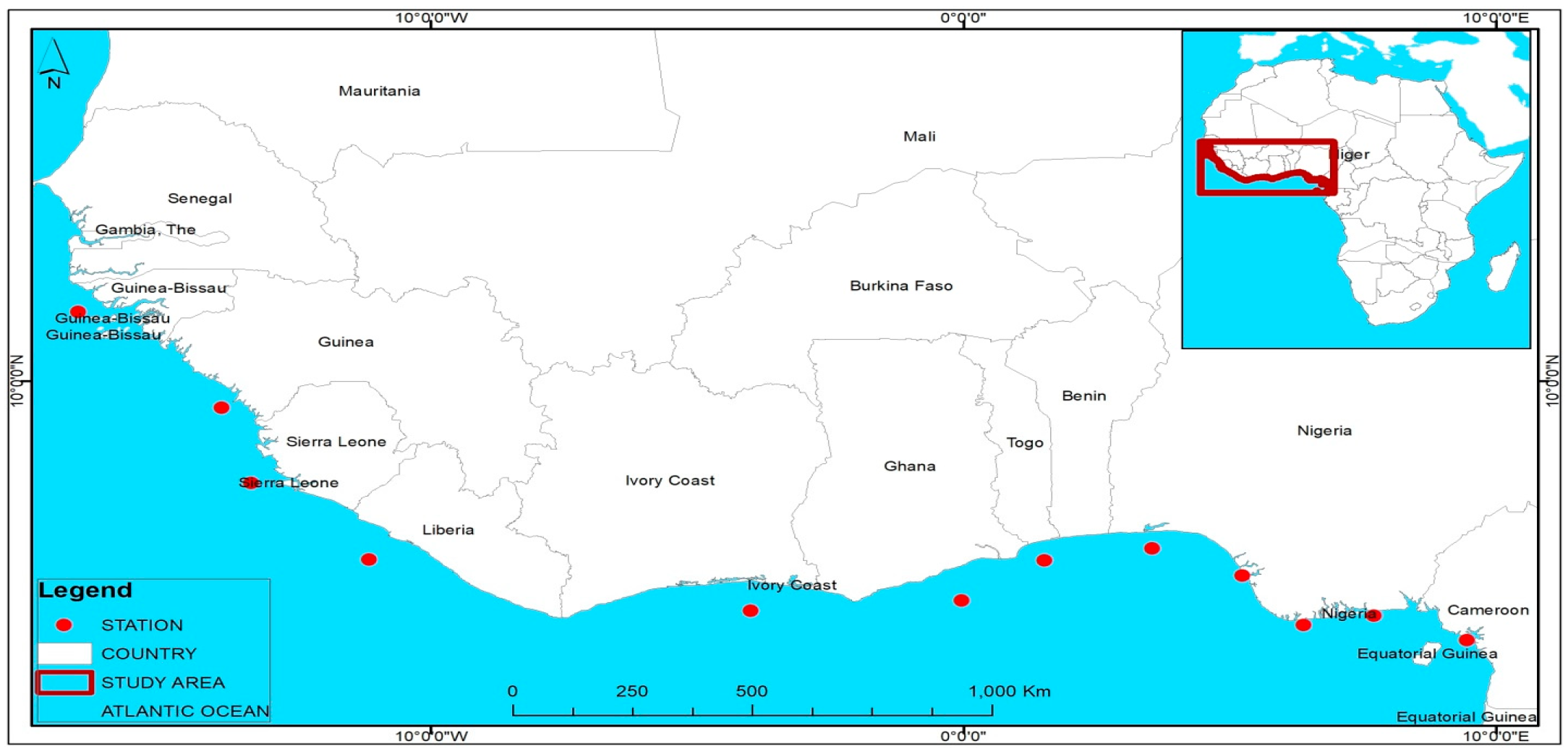
The study area is the GOG region located in the southeast of the Atlantic Ocean . The area lies between longitudes 10 °W and 8 °E and latitudes 5 °N and 5 °S, and thus, south of West Africa as shown in
Figure 1. The hydrography of the GOG is directly affected by five main currents, namely, Benguela, the South Equatorial, the Canary, the Counter Equatorial, and the Guinea Currents (Odekunle and Eludoyin,2008).
The tropical marine (mT) air mass and the tropical continental (cT) air mass are the two main wind currents that have the most impact on the climate of GOG and all of West Africa. The Equatorial Easterlies, a third wind current, is only significant over the continent of West Africa (Ojo, 1977; Iloeje, 1981). The southern high-pressure band off the coast of Namibia is where the mT air mass starts. On its path, the air mass takes up moisture over the South Atlantic Ocean, crosses the Equator, and then penetrates GOG and West Africa. The high-pressure area to the north of the Tropic of Cancer is where the cT air mass is found. It picks up little moisture along its path and is thus dry. The two air masses (mT and cT) meet along a slanting surface called the Inter-tropical Discontinuity (ITD). The Equatorial Easterlies are rather erratic cool air masses, which come from the east and flow in the upper atmosphere along the ITD.
3. Results And Discussion
3.1. Historical/Observed SST Climatology
Attempt is made here to examine the pattern of observed SST (1940-2014) before proceeding to evaluate CMIP6 bias corrected future projection (2030-2100). The individual model projection is discussed as follow:
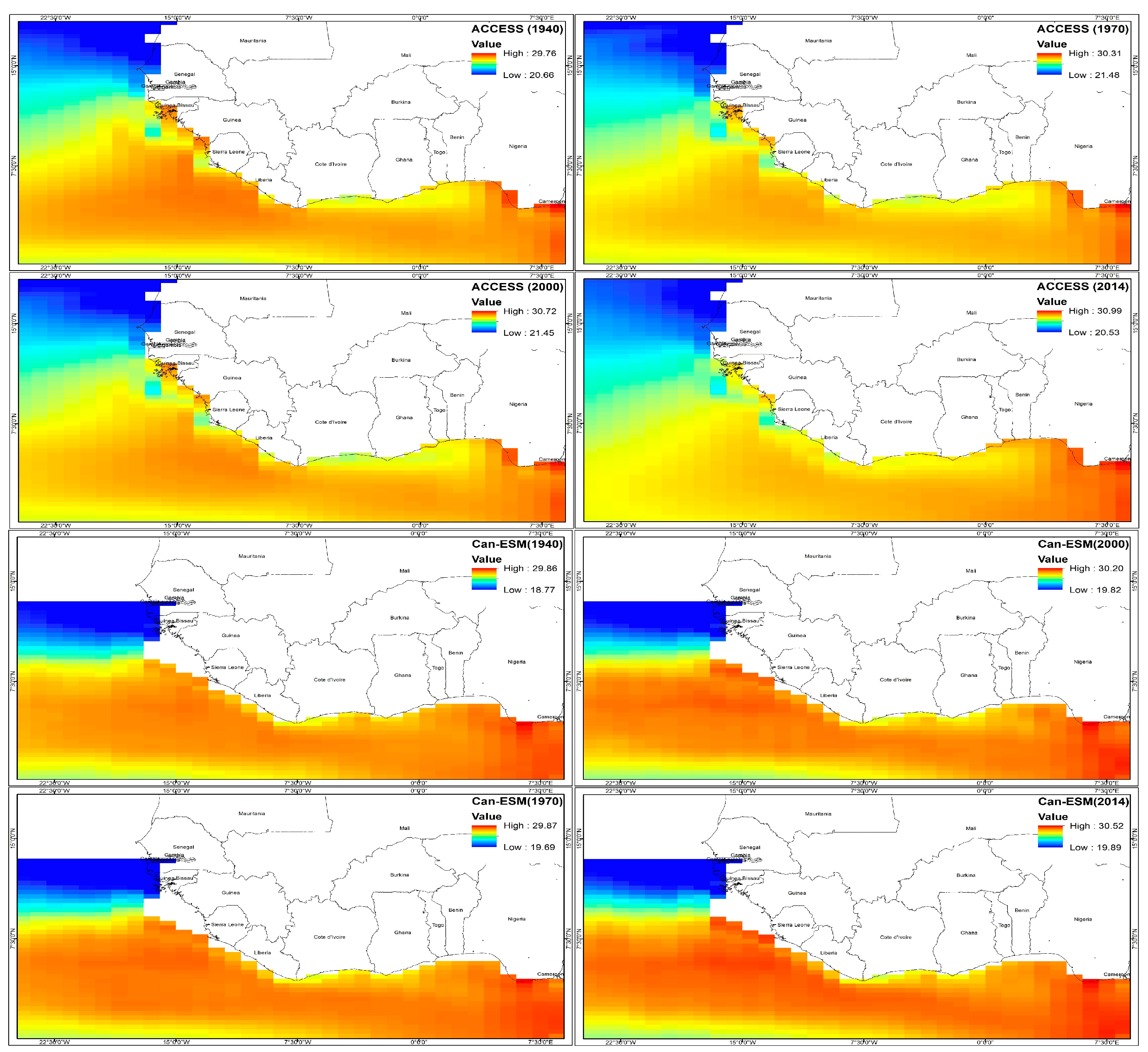
The observations by ACCESS-CM2 as shown in
Figure 2 in 1940 for the GOG indicates 29.76
oC for the high warming GOG and 20.66
oC for the low. In 1970, the model captured 30.31
oC for the Guinean coast and 21.48 for the Western Sahel (Low) while in 2000, 20.72
oC was simulated for the warming regions of the GOG and 21.45
oC. The observed SST for 2014 for the Guinea Coast has 30.96
O as sea surface temperature and 20.53 for the Western Sahel respectively.
The interannual change of the historical SST climatology as revealed by ACCESS-CM2 is 1.23oC as shown in Figure 17 below while that of the Western Sahel is 0.13oC with most of the warming in 1970 and 2000 for the western Sahel while the year 2014 was remarkable as it recorded the highest (30.99o) in the Guinean Coast.
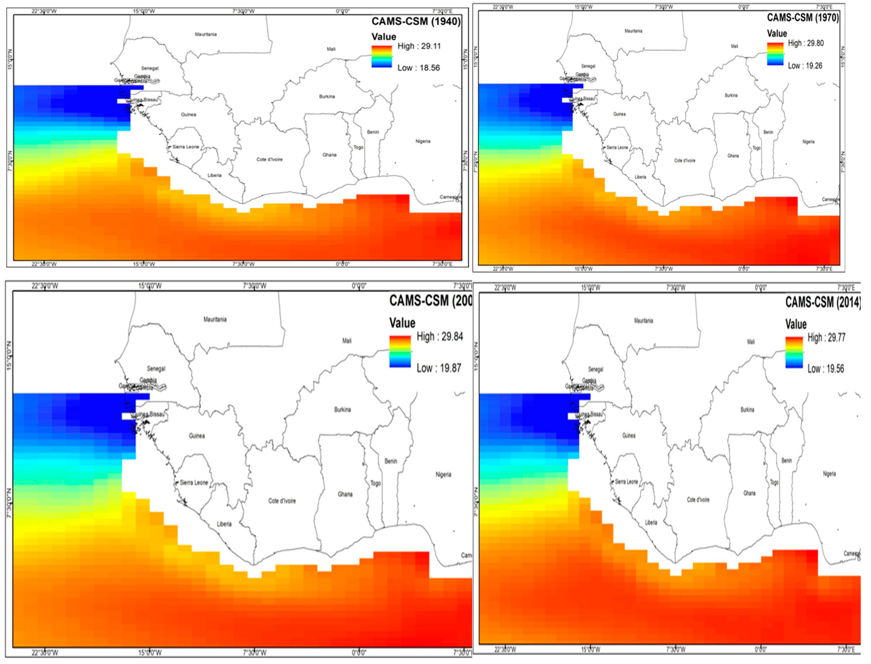
CAMS-CSM1-0 shown in
Figure 3 below captured the mean SST Climatology in 1940 as 29.11
oC for the high warming GOG region and 18.56
oC for the low while in 1970, SST was 29.80
o and 19.26
o for the high and low respectively. In 2000, the historical SST mean was shown as 29.84
o and 19.87
o for the low.
In 2014, the high warming region recorded 29.77
oC and 19.56
oC for the low indicating that SST increased by 0.66
o between 1940-2014 for the Guinean coast and the 0.18
oC for the low (Western Sahel). The historical pattern of SST mean climatology as demonstrated by Can-ESM5 in
Figure 2 is consistent as the model captured 29.86
oC for 1940 and 18.77
oC for the low. In 1970, the mean SST recorded was 29.87
oC for the high warming region and 19.69
oC for the Western Sahel. Increased warming was further observed in 2000 as SST was put at 19.82
oC in the low. The pace of accelerated SST continued in 2014 as the high warming regions of the GOG recorded 30.52
oC and 19.89
o for the low. On the Average, SST increased by 0.66
oC in the GOG and 1.12
oC for the Western Sahel.
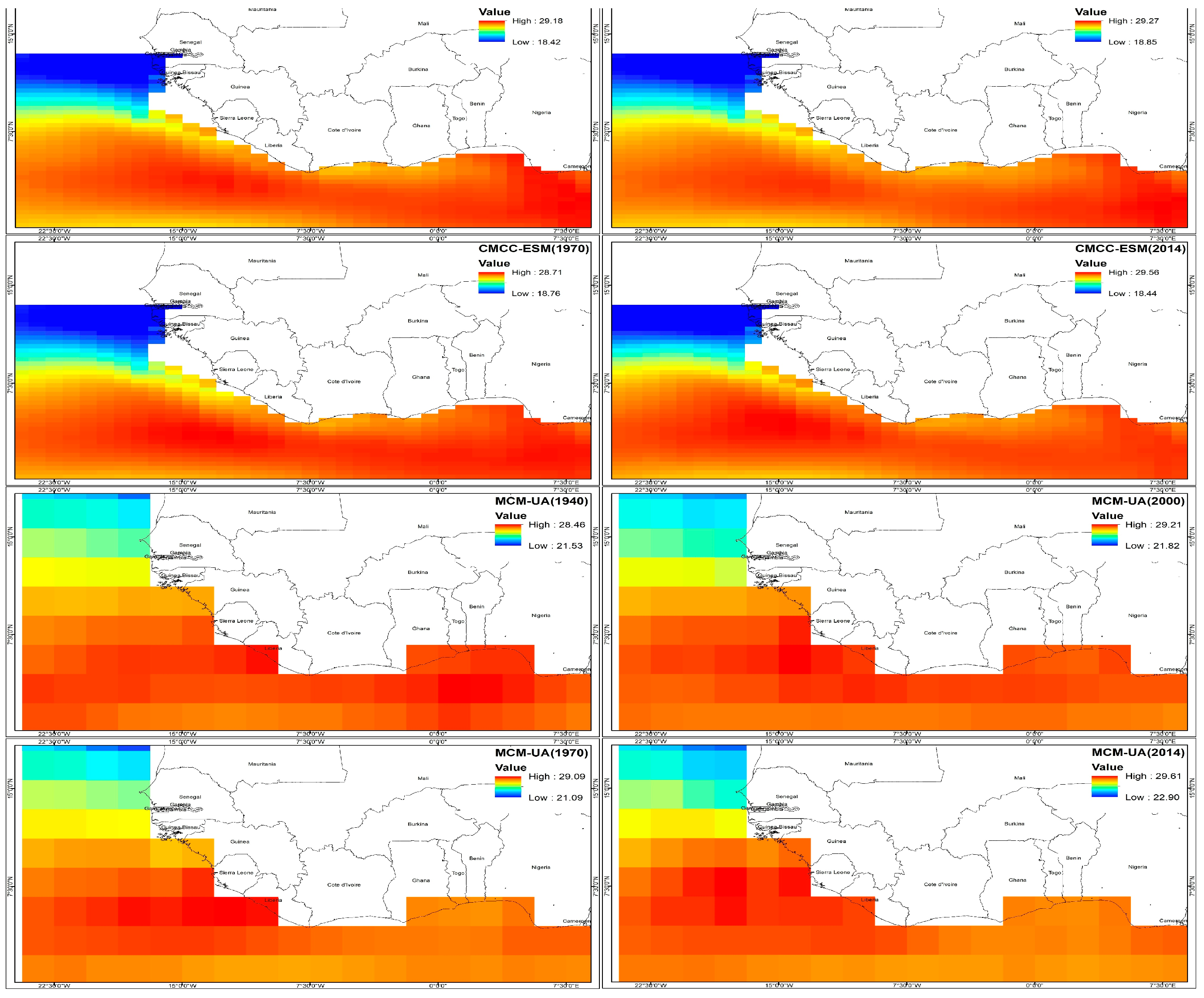
CMCC-ESM model simulation of the historical SST of the GOG in 1940 shown in
Figure 5 has 29.18
oC for the high and 18.42
oC in the Western Sahel. The 1970 mean SST value for the high however contrasted with 28.71
oC for the high and 18.76
oC for the low. The year 2000 saw an upward increase in the mean SST of the Gulf of Guinea as the high recorded 29.27
oC and 18.46
oC for the high and low. The biggest increase was in 2014 with 29.56
oC and 18.44
oC for the high and low.
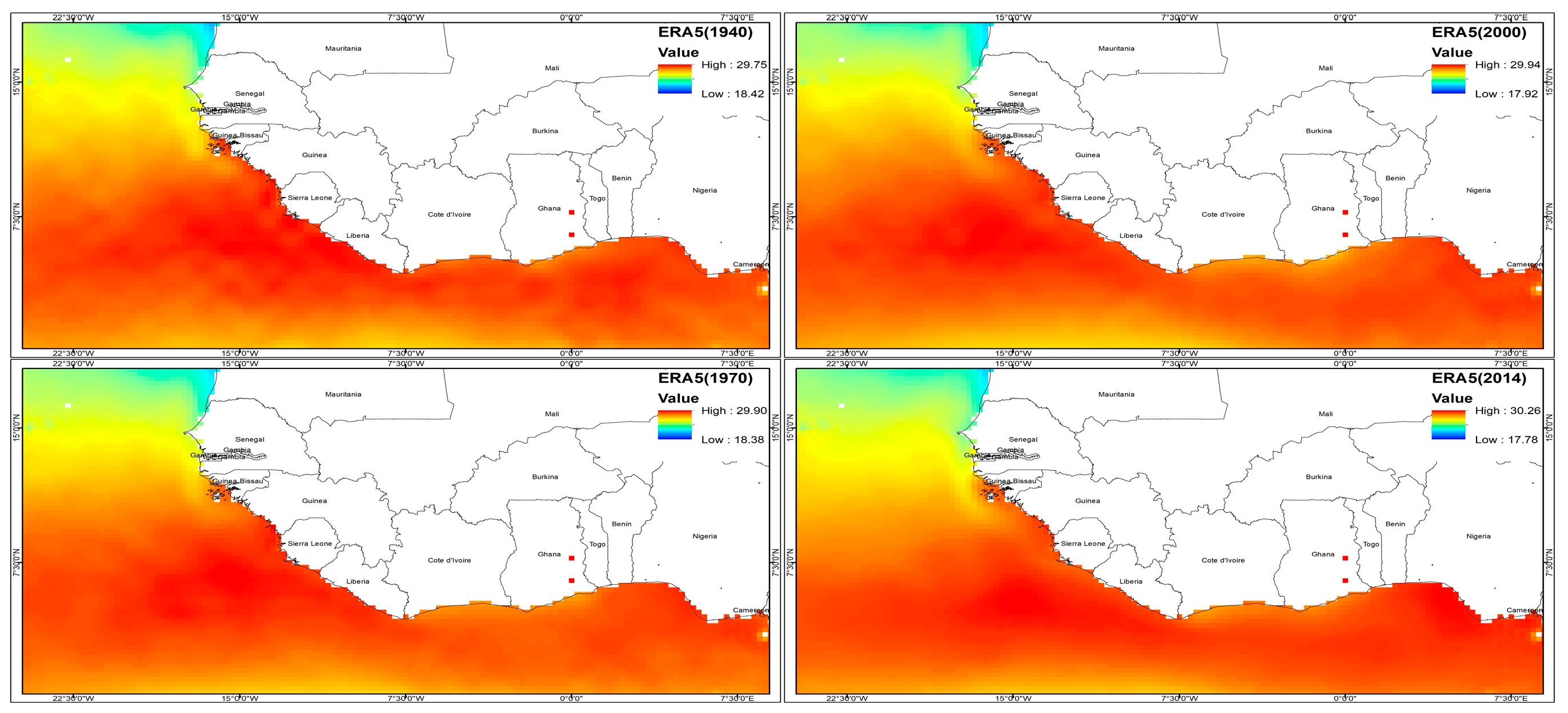
Similarly, the ERA5 as shown in
Figure 4 which is the observed data indicate that in 1940, the mean SST was 29.75
oC for the high and 18.42
o for the low while in 1970, significant increase in mean SST was recorded with 29.80
oC for the high and 18.38
oC for the low. Again in 2014, the ERA5 SST captured mean SST as 30.25
oC for the high and 17.78
oC for the low implying SST increased by 0.55
oC during the period.
MCM-UA model evaluation of the SST historical data as shown in
Figure 5 indicates 28.46
oC in 1940 for the high and 21.53
oC for the low while an increasing trend was observed in 1970 with 29.09 for the high and 21.09
oC for the low. In 2000, the increasing SST trend continued for the high and low with 29.21
oC and 21.82
oC. The pattern of observation was not different in 2014 as the individual model captured 29.61
oC been the highest the high warming region of the GOG and 22.90
oC for the low,
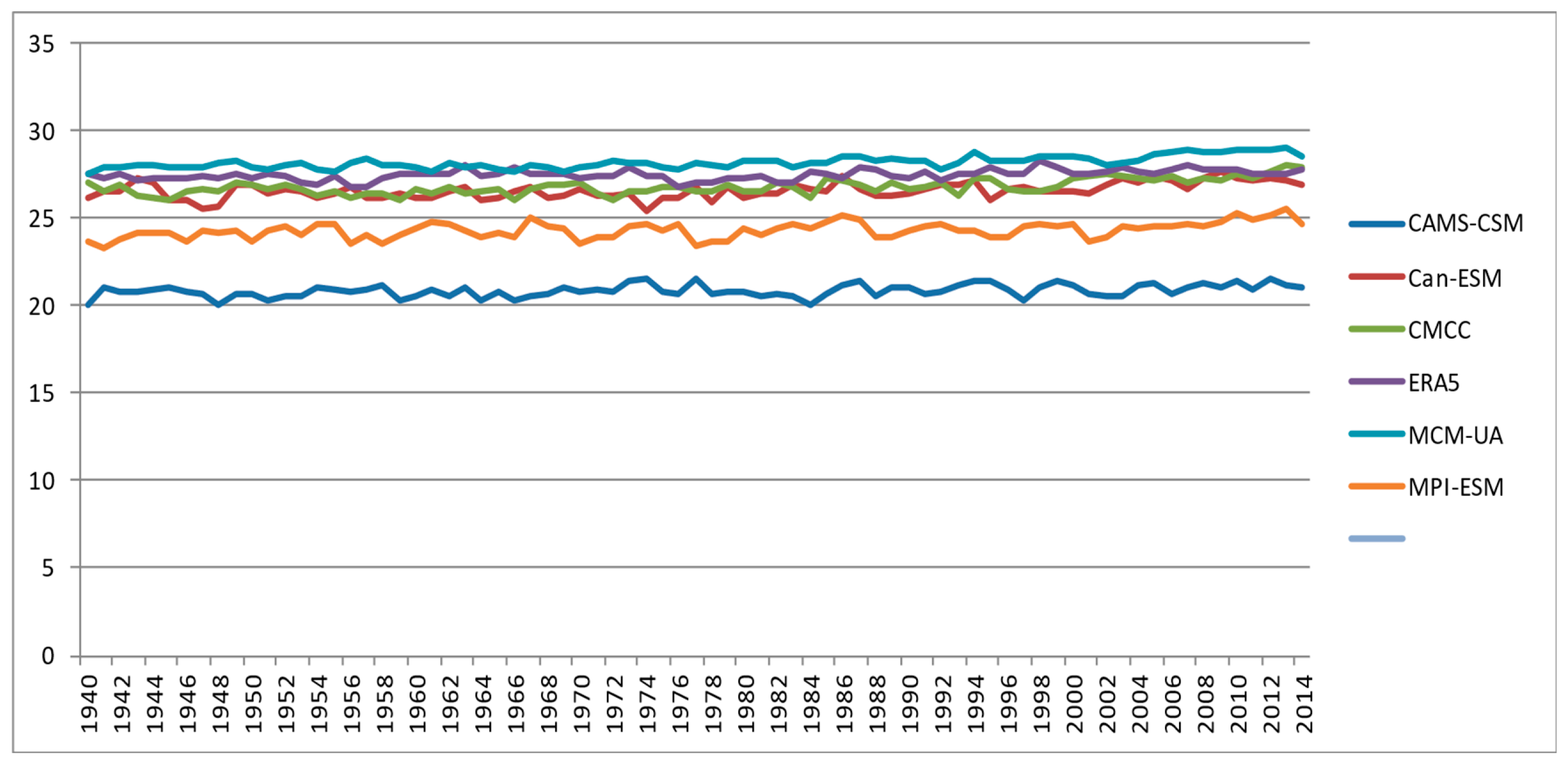
Arising from the results above, it is evident that SST increased by an average of 1.15oC between 1940-2014 for the GOG and 1.37oC for the low warming region (Sahel). This further indicates that all the model ensembles were consistent in capturing the interannual variability of the mean SST climatology with some level of accuracy.
3.2. CMIP6 Future SST projection
Bias corrected CMIP6 climate models derived from GCM data using EQM for the simulated future SST pattern is presented below based on RCP 8.5 for the GOG and Western Sahel. Having presented the SST historical pattern above, the decadal projection of the SST from 2030-2100 is hereby discussed as follows.
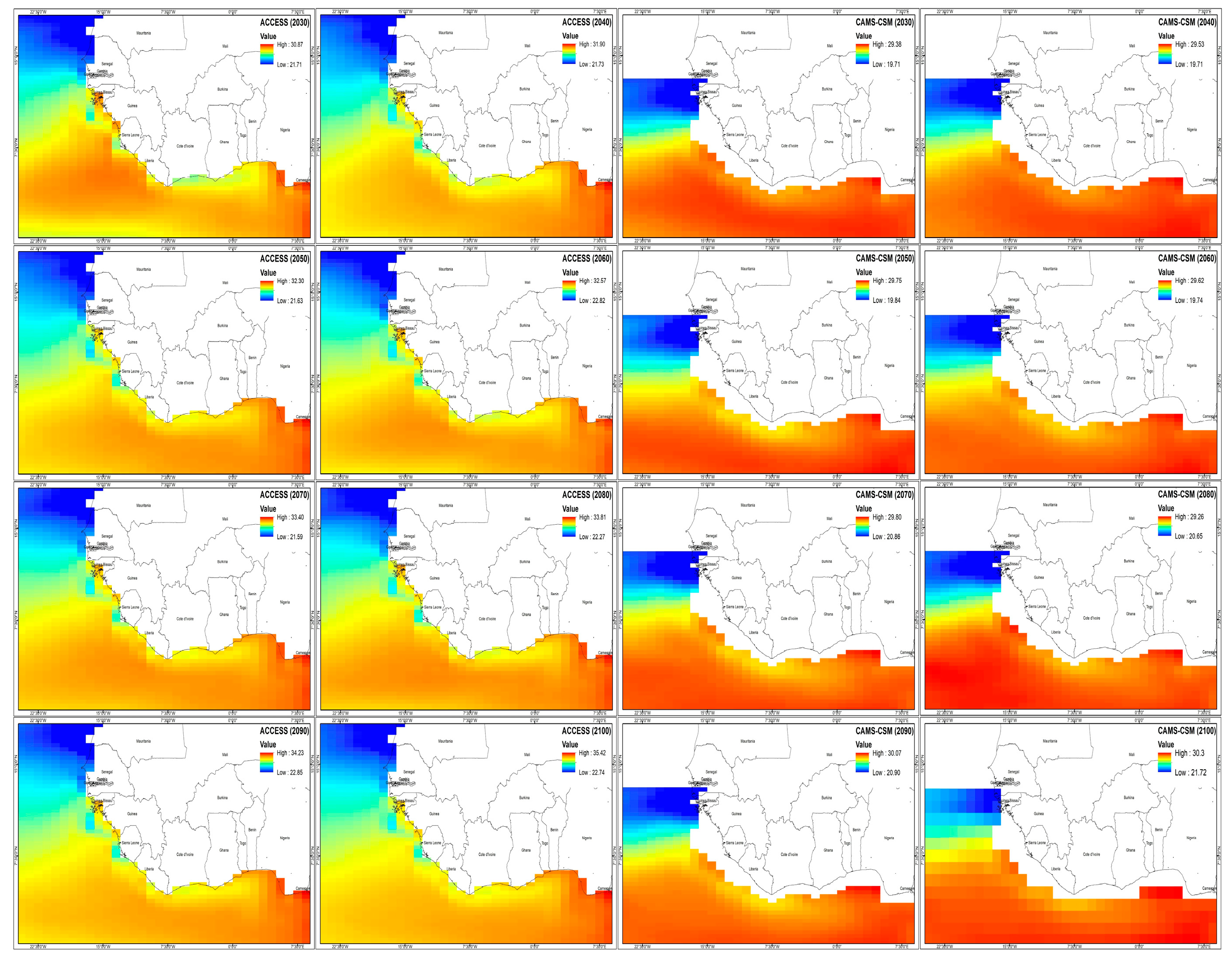
ACCESS-CM2 future SST simulation of 2030 for the high warming region of the GOG shown in
Figure 6 below is projected to be 30.87
oC and 21.77
oC for the Western Sahel. In 20140, further significant warming was projected for the high as 31.90
oC and 21.73
oC for the low while the 2050 projection puts SST as 32.30
oC and 21.63
oC for both the high and low.
The projected warming is expected to continue unbated with the individual model posting 32.57oC for the high and 22.82oC for the low while the 2070 model projection indicates 32.40oC and 21.58oC for the high and low respectively. The 2080 model projection captures mean SST of the high as 33.81oC and 22.27oC for the low and the upward warming swing is projected to continue in 2090 with 34.23oC for the high and 22.85oC for the low, the individual model projection in 2100 is expected to recorded the highest with 35.42oC and a cold tongue with 22.74oC. The accelerated warming and increased SST projected by this model implies the intensification of increased extreme climate events given the role of ocean-atmosphere feedback and ENSO mechanism (Sasaki, et al, 2015, Fang and Huang 2019, Null, 2019 and Bulgin, et al 2020)
CAMS-CSM output as shown in
Figure 6 captures future projection of mean SST in 2030 for the high warming is 29.38
oC and 19.71
oC for the low warming regions of the GOG with further increase expected in 2040 as the high will record 29.53
oC and a wet bias of 19.71
oC. Additional warming of 29.75
oC and 19.84
oC will be recorded in 2050 for the high and low while the SST variability in the 2060 projection will see the GOG experience 29.62
oC and 19.74
OC for the high and low. The future SST projection for 2070 is expected to be significantly warmer than 2060 given the variability values of 29.82
oC and 20.86
oC for both the high and low and 29.26
oC and 20.85
oC in 2080. The year 2090 is projected to be warmer with 30.07
oC and 20.90
oC for the high and low with 2100 recording 30.3
oC for the high and 21.72
oC for the low regions of the study area.
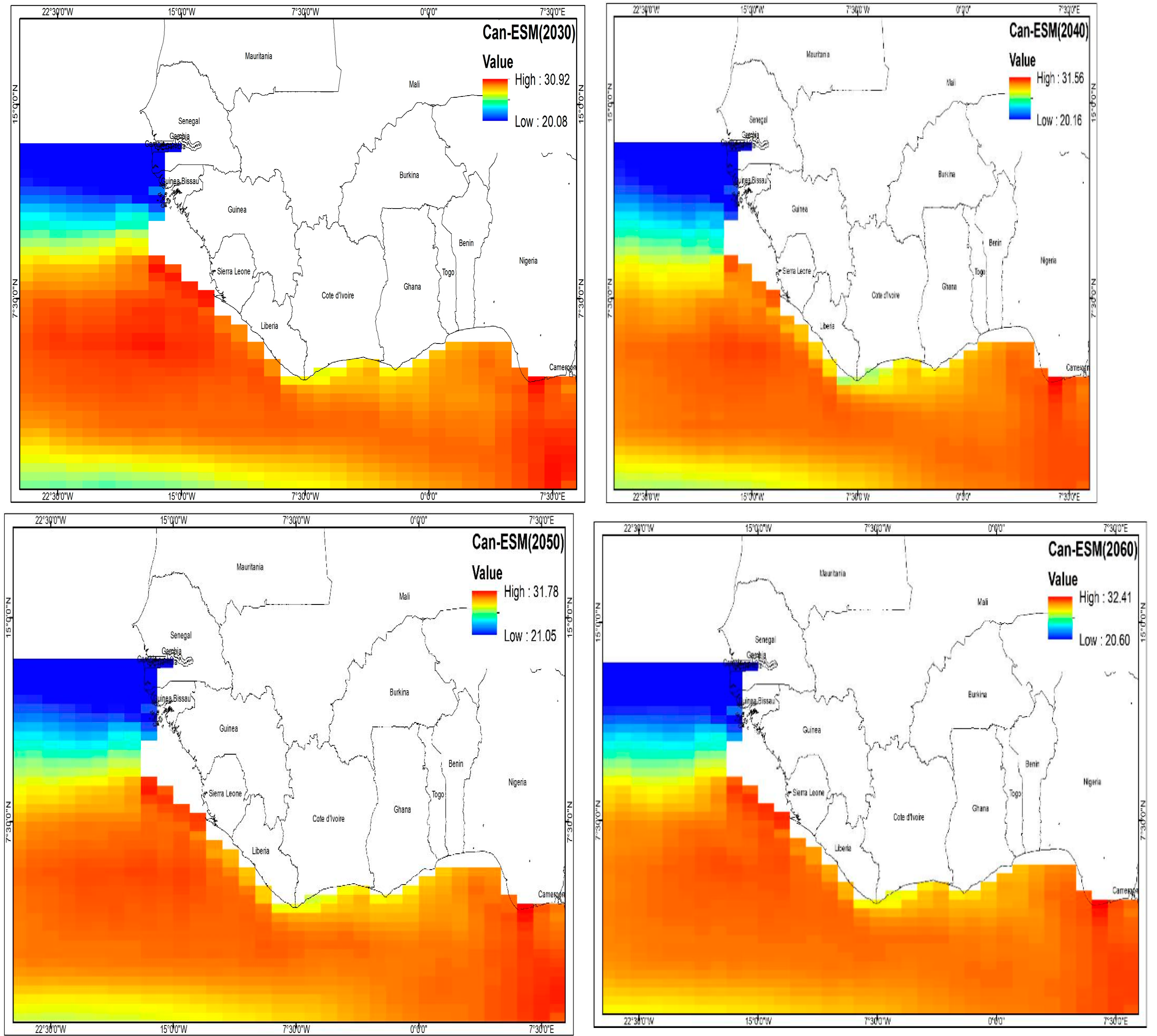
The model simulation of future SST by CAM-ESM in 2030 shown in
Figure 7a and b above is projected to be 30.82
oC and 20.08
oC for the high and low respectively while in 2040, 31.56
oC and 21.16
oC is projected for the high and low, Increasing significant warming is projected in 2050 and 2060 with 31.78
oC and 21.05
oC for the high and low and 32.41
oC and 20.80
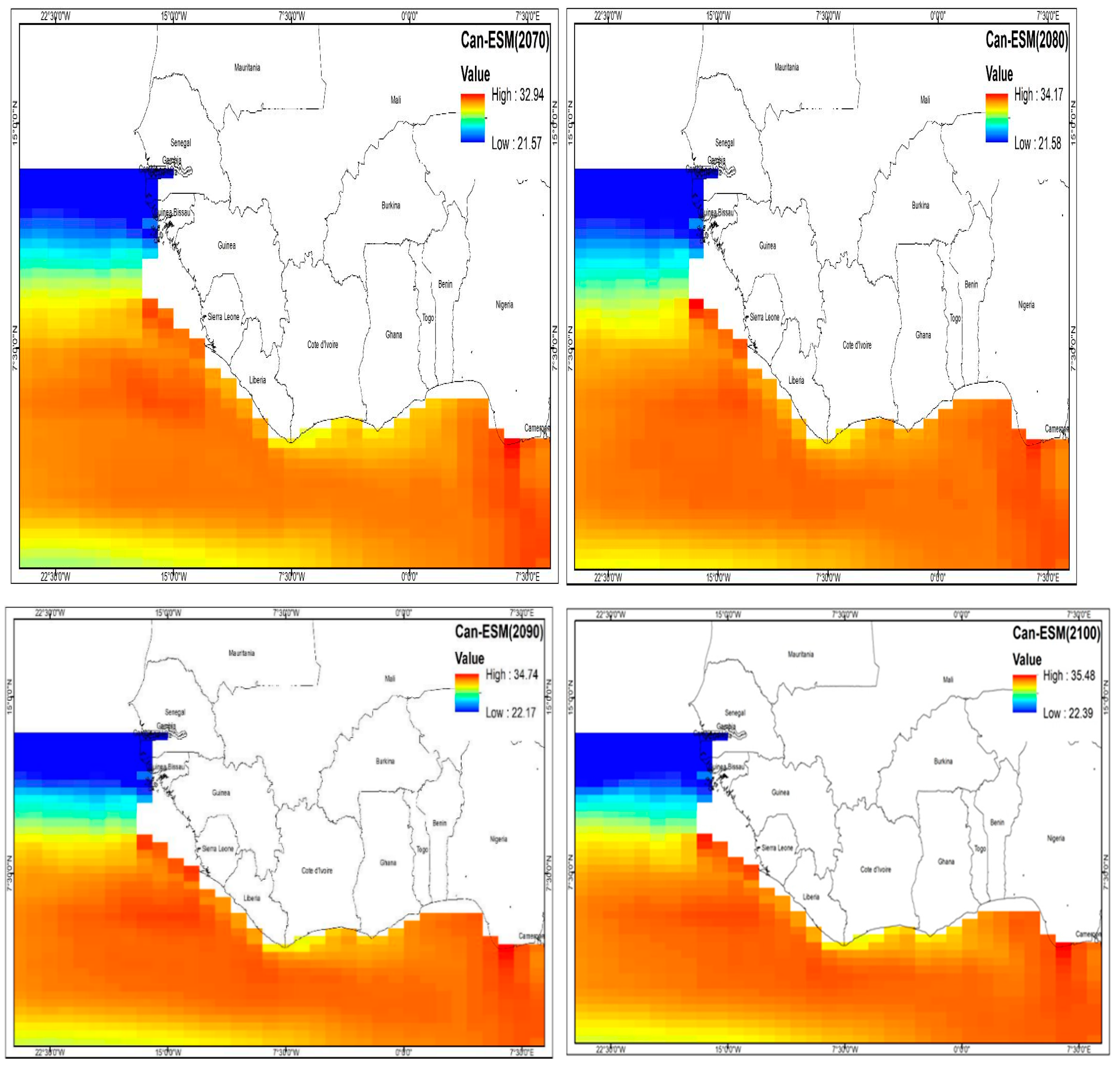
oC (2060, high and low) respectively. In 2070, the warming pattern of the ocean is projected to continue with 32.94
oC and 21.57
oC for the high and low regions of the GOG with a further warming projection of 34.17
oC and 21.58
oC respectively. 2090 is projected to be significantly warmer with 34.74
oC for the high and 22.117
oC for the low. The year 2100 is projected to experience a record ocean warming with mean SST of 35.45
oC and 22.30
oC.
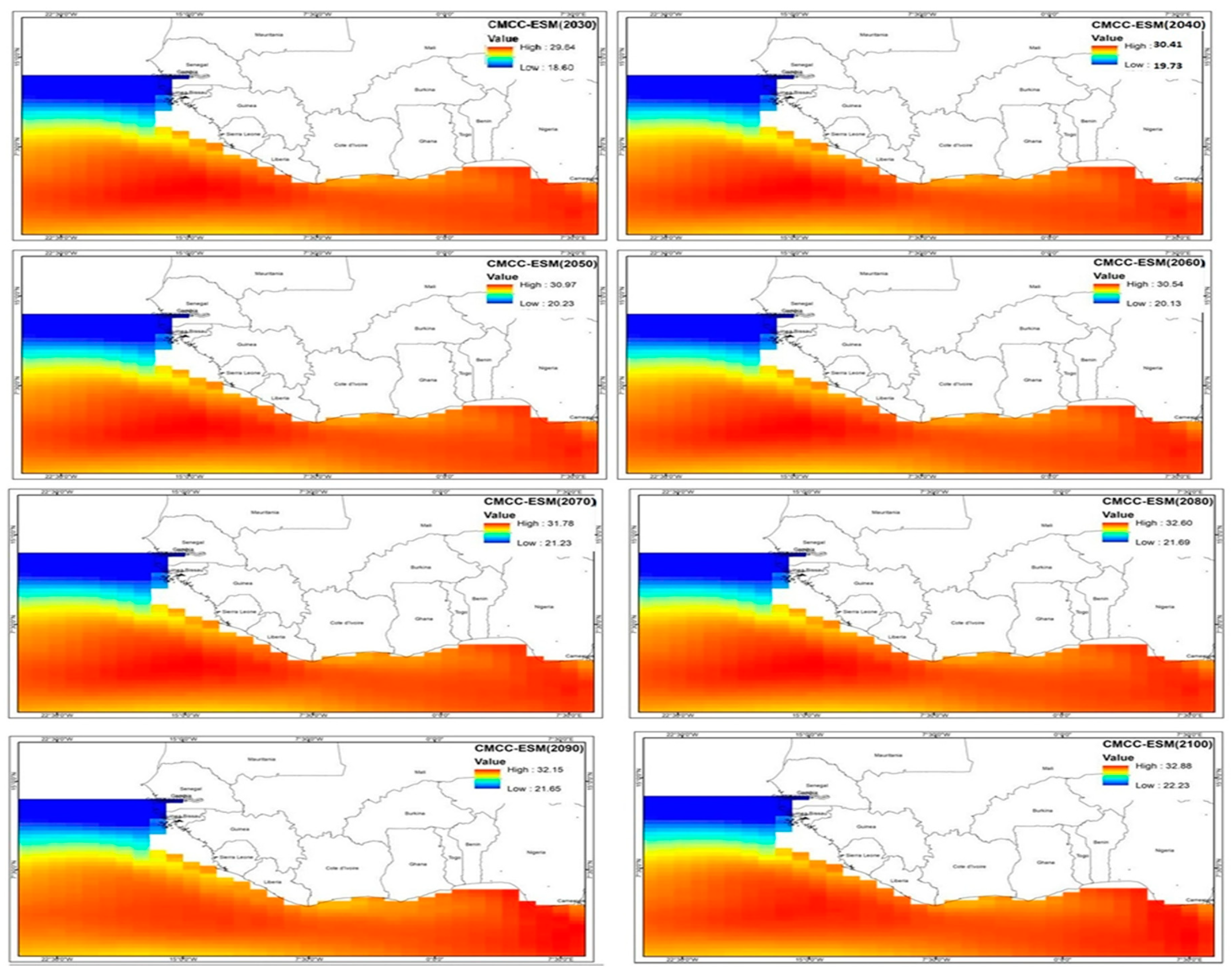
The CMCC CMIP6 bias corrected simulation of future SST of the GOG for 2030 shown in
Figure 8 projects SST to be 29.64
oC and 18.80
o for the high warming and the Western Sahel regions. A further warming bias is projected in 2040 with 30.41
oC and 18.73
oC for the high and low. The model further project future SST in 2050 be 30.87
oC while the low is projected to be 20.23
oC. Additional warming bias is projected in 2060 to be 30.54
oC and 20.13
oC. The model projection for 2070 by CMCC-ESM to be 31.78
oC and 21.23 for both the high and low respectively. The projection for 2080 is expected to be considerably higher than 2070 with 32.60
oC for the warning coastal region of the GOG and 21.69
oC for the Western Sahel. Future SST projection in 2090 is expected to be lower than 2080 for the GOG with 32.15
oC for the high and 21.65
o for the low. In 2100, significant warming and increased SST variability is projected in the GOG with 32.88
Oc and 22.23
oC for the high and low respectively.
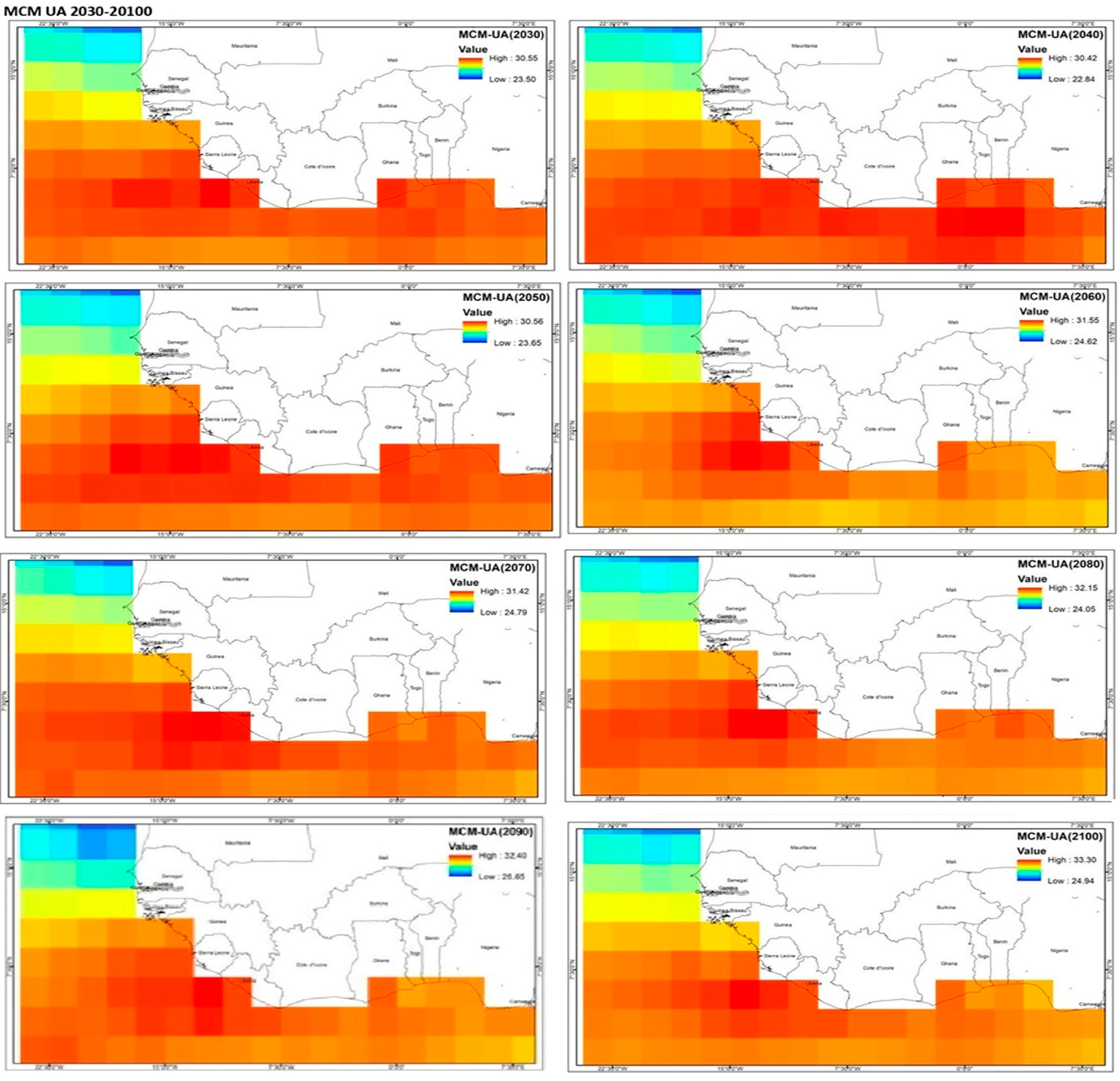
Relatedly, MUCM-UA shown in
Figure 9 above projects a warming bias of 30.55
oC as mean SST for the Guinean Coast and 22.50
oC for the Western Sahel. In 2040, a cold bias is projected for the high with 30.42
o while a warm bias is expected in the Western Gulf of Guinea. MCM further captures the future SST projection in 2050 as 30.56
oC and 23.65
oC for the high and low. 2060 is projected to be significantly warmer than the preceding year with 31.55
oC for the high and 24.62
o for the low. Reduce warming and cold tongue is projected for the high in 2070 with 3.42
oC for the high while the western flank of the GOG is projected to be slightly warmer with 24.79
oC. Sustained SST warming is projected in 2080 with the high recording 32.15
oC and 24.05
o for the low. The model SST future projection of the Gulf of Guinea in 2090 has 32.40
oC for the high and 26.65
oC for the low indicating that the low will be significantly warmer. Increased warming bias is further projected in 2100 as the high will warm by 33.3
oC and a cold bias in the low with 24.90
o
4. Discussion of Findings
The spatial climatology of the historical data (1940-2014) and the CMIP6 simulations (2030-2100) were presented in the preceding section. It is important to emphasize that most of the models successfully reproduced the spatial pattern of SST over the GOG and the Western Sahel, However, the highest SST value was produced by CAM-ESM (35.48oC and 22.39oC indicating that the model over estimated SST climatology while the lowest values was in 2030 (29.38o and 19.71OcC ) implying the persistence of a warming bias in the Guinean cost and cold tongue along the western Sahel and underestimation of SST. The presence of these results clearly shows the influence of ENSO as the dominant driver of SST variability as evidenced in the warm bias and cold tongue in the Western flank of the Guinean coast. This implies that all the models overestimated SST in the Guinean coast when juxtaposed with the observed data set. The historical ERA5 data was used to validate the projected changes in the SST and as shown in the simulation, the bias corrected data was consistent with the observed data for the climatological mean period.
Findings from the CMIP6 model simulation further revealed that SST is projected to increase by 1.03oC between 2030 and 2040 in the Western GOG with most of the warming projected to occur in 2090 and 2100. The projected warming bias demonstrated by the CMIP6 models are not surprising as RCP 8.5 assumes higher GHG emission (Jose,2021). Similarly, SST in the Guinean coast reputed for its high warming is projected to increase by 4.61oC between 2030 and 2100 with SST expected to be substantially higher in the far end than the near period in the study domain, although the projected warming is not homogenous as substantial increases in the multimodal mean SST is expected more in the Guinea coast than the Western Sahel. Similarly, Roehrig et al,2013 in their studies of bias corrected CMIP 3 and CMIP 5 affirmed that coupled models exhibit sizable biases in the mean position of the West African Monsoon. Furthermore, the outcome of their analysis revealed that most models contain a warm bias in the equatorial Atlantic, and a southward shift of the ITCZ in coupled models; this southward bias was also examined in other studies conducted by (Siongco et al. 2015; James et al. 2018; Steinig et al. 2018). Other studies that have been carried out using GCM CMIP simulation include those of Dunning et al. (2017) who asserts that the Coupled Model Intercomparison Project Phase 5 (CMIP5) historical simulations underestimated SST seasonal cooling from April/May to August over the northern Gulf of Guinea and suggested that might have been driven by incorrect seasonality of precipitation over the southern coastline of West Africa. Similar studies conducted by (Brown et, al 2015) on projected sea surface temperature over the equatorial pacific posits that the warm pool region is projected to experienced enhanced warming along the equatorial Pacific. Overall, future SST of the GOG is projected to become warmer in the future and the magnitude of change will depends on future GHG scenarios. The projected warming produced in this study could impact on marine ecosystem, fishes, and the local climate.
4.1. Statistical Evaluation of CMIP6 Model performance
This section examines the ability of the CMIP6 models to simulate the observed historical simulation. Several methods of validating the performance of GCM driven CMIP6 simulation exist in the literature, and it include Nash-Sutcliffe efficiency (NSE), the Root-Mean square Error (RMSE) or the Root mean square Deviation (RMSD), the mean absolute Error (MAE), the Percentage bias (PBIAS) and the correlation coefficient (Cr). These techniques have been employed my different researchers for validation of bias corrected CMIP6 simulation (Bhatt, et al,2016, Meendez, at al 2020 and Cai et al, 2021, Rhymee at al 2021). However, in this study, the performance of the GCM-CMIP6 in simulating the observed data set was evaluated using the correlation coefficient. Consequently, the ability of each of the models used in the study in reproducing the spatial pattern of SST over the GOG was evaluated/validated against the ERA5 reanalysis data from 1940-2014 using statistical analysis.
Regression analysis is very useful when it comes to studying the relationship between variables. Regression analysis can identify the cause and effect of one variable to another variable. Variables are the main part in regression analysis. There are dependent variables (or criterion variable) and independent variable (or predictor variable). In multiple regression, the independent variables can be added more in the model to explain the cause and effect of dependent variables. Hence, dependent variables can be predicted by building better models using multiple regression analysis.
4.2. Multiple Regression
Multiple regression models can be presented by the following equation:
Where 𝑌 is the CanESM (dependent variable), 𝑋1,2, 𝑋3,𝑋4and 𝑋5 (independent variables) are ACCESS, CAMS-CSM, CMCC-ESM, EC-Earth3, MCM-UA and MPI-ESM respectively. 𝛽1, 𝛽2, 𝛽3, 𝛽4 and 𝛽5 are model coefficients of the six independent variables. 𝑏0 is a constant while 𝜀 is the error.
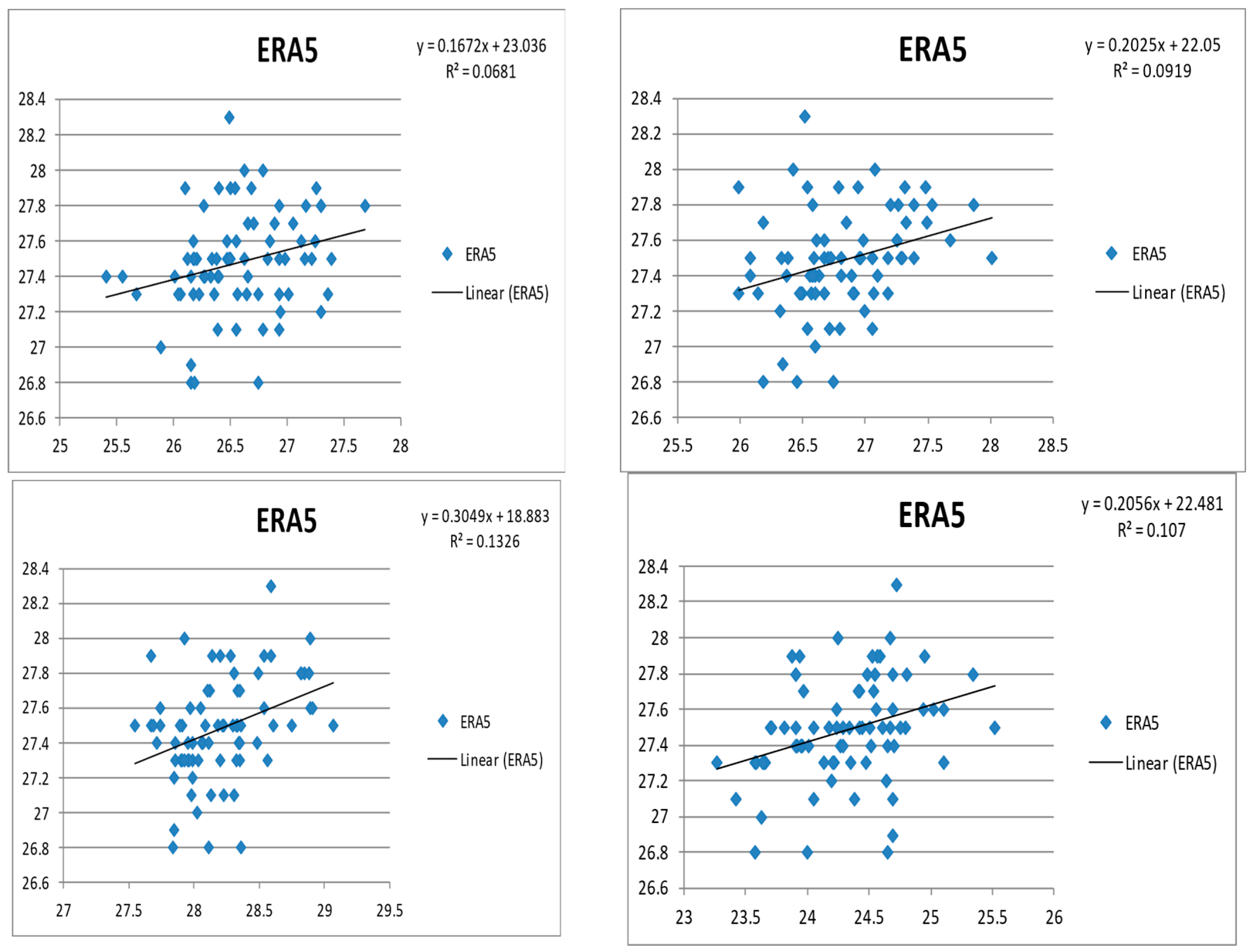
The outcome of the model regression analysis conducted as shown in
Figure 10 and
Figure 11 below indicates that the all models namely ACEES, CAMS-CSM. CAN-ESM, CMCC, MUM and MP-ESM have R values of 0.10, 0.01, 0.06. 0.09, 0.10 and 0.013 respectively. The weakest correlation is CAMS-CSM model 0.01 while the strongest correlation is MUM-UA with 0.13 given the fact that the closer r is to +1, the stronger the correction between the variables of interest while -1 implies negative correlation. The summary regression statistic further indicates that there is a positive correlation between the individual models and the ERA historical data of 1940-2014.
4.3 Test of significance
The Pearson product moment correlation coefficient (r) carried out on the CMIP6 models to validate the performance of the model indicates that that ACESS, CAMS-CSM, CAN-ESM, CMCC and MUM UA were statistically significant at 1 tailed significance test with the r values of 0.00,0.00,0.00,0.00, and 0,00 at 0.00 (P < 0.05) as shown in
Table 4 below. This implies that the individual models performed well and therefore suitable for in simulating the statistical pattern of SST over the Gulf of Guinea.
Table 3.
Coefficient of Correlations.
Table 3.
Coefficient of Correlations.
| |
ERA5 |
ACCESS |
CAMS |
CanESM |
CMCC |
MCM |
|
| Pearson Correlation |
ERA5 |
1.000 |
.318 |
.136 |
.261 |
.303 |
.364 |
|
| ACCESS |
.318 |
1.000 |
.378 |
.318 |
.522 |
.497 |
|
| CAMS |
.136 |
.378 |
1.000 |
.230 |
.274 |
.466 |
|
| CanESM |
.261 |
.318 |
.230 |
1.000 |
.463 |
.525 |
|
| CMCC |
.303 |
.522 |
.274 |
.463 |
1.000 |
.559 |
|
| MCM |
.364 |
.497 |
.466 |
.525 |
.559 |
1.000 |
|
| MPI |
.327 |
.177 |
.241 |
.349 |
.399 |
.460 |
|
| Sig. (1-tailed) |
ERA5 |
. |
.003 |
.122 |
.012 |
.004 |
.001 |
|
| ACCESS |
.003 |
. |
.000 |
.003 |
.000 |
.000 |
|
| CAMS |
.122 |
.000 |
. |
.024 |
.009 |
.000 |
|
| CanESM |
.012 |
.003 |
.024 |
. |
.000 |
.000 |
|
| CMCC |
.004 |
.000 |
.009 |
.000 |
. |
.000 |
|
| MCM |
.001 |
.000 |
.000 |
.000 |
.000 |
. |
|
| MPI |
.002 |
.065 |
.018 |
.001 |
.000 |
.000 |
|
| N |
ERA5 |
75 |
75 |
75 |
75 |
75 |
75 |
|
| ACCESS |
75 |
75 |
75 |
75 |
75 |
75 |
|
| CAMS |
75 |
75 |
75 |
75 |
75 |
75 |
|
| CanESM |
75 |
75 |
75 |
75 |
75 |
75 |
|
| CMCC |
75 |
75 |
75 |
75 |
75 |
75 |
|
| MCM |
75 |
75 |
75 |
75 |
75 |
75 |
|
| MPI |
75 |
75 |
75 |
75 |
75 |
75 |
|
| Model Summaryb |
| Model |
R |
R Square |
Adjusted R Square |
Std. Error of the Estimate |
Durbin-Watson |
|
| 1 |
.364a |
.133 |
.121 |
.274 |
1.376 |
|
| a. Predictors: (Constant), MCM |
|
| b. Dependent Variable: ERA5 |
|
| ANOVAa |
|
| Model |
Sum of Squares |
df |
Mean Square |
F |
Sig. |
|
| 1 |
Regression |
.837 |
1 |
.837 |
11.161 |
.001b |
|
| Residual |
5.477 |
73 |
.075 |
|
|
|
| Total |
6.314 |
74 |
|
|
|
|
| a. Dependent Variable: ERA5 |
|
| b. Predictors: (Constant), MCM |
|
| Coefficients |
|
| Model |
Unstandardized Coefficients |
Standardized Coefficients |
t |
Sig. |
|
| B |
Std. Error |
Beta |
|
| 1 |
(Constant) |
18.883 |
2.574 |
|
7.336 |
.000 |
|
| MCM |
.305 |
.091 |
.364 |
3.341 |
.001 |
|
| Coefficients |
| Model |
95.0% Confidence Interval for B |
Correlations |
Collinearity Statistics |
| Lower Bound |
Upper Bound |
Zero-order |
Partial |
Part |
Tolerance |
| 1 |
(Constant) |
13.753 |
24.013 |
|
|
|
|
| MCM |
.123 |
.487 |
.364 |
.364 |
.364 |
1.000 |
| Coefficientsa |
| Model |
Collinearity Statistics |
| VIF |
| 1 |
(Constant) |
|
| MCM |
1.000 |
| a. Dependent Variable: ERA5 |
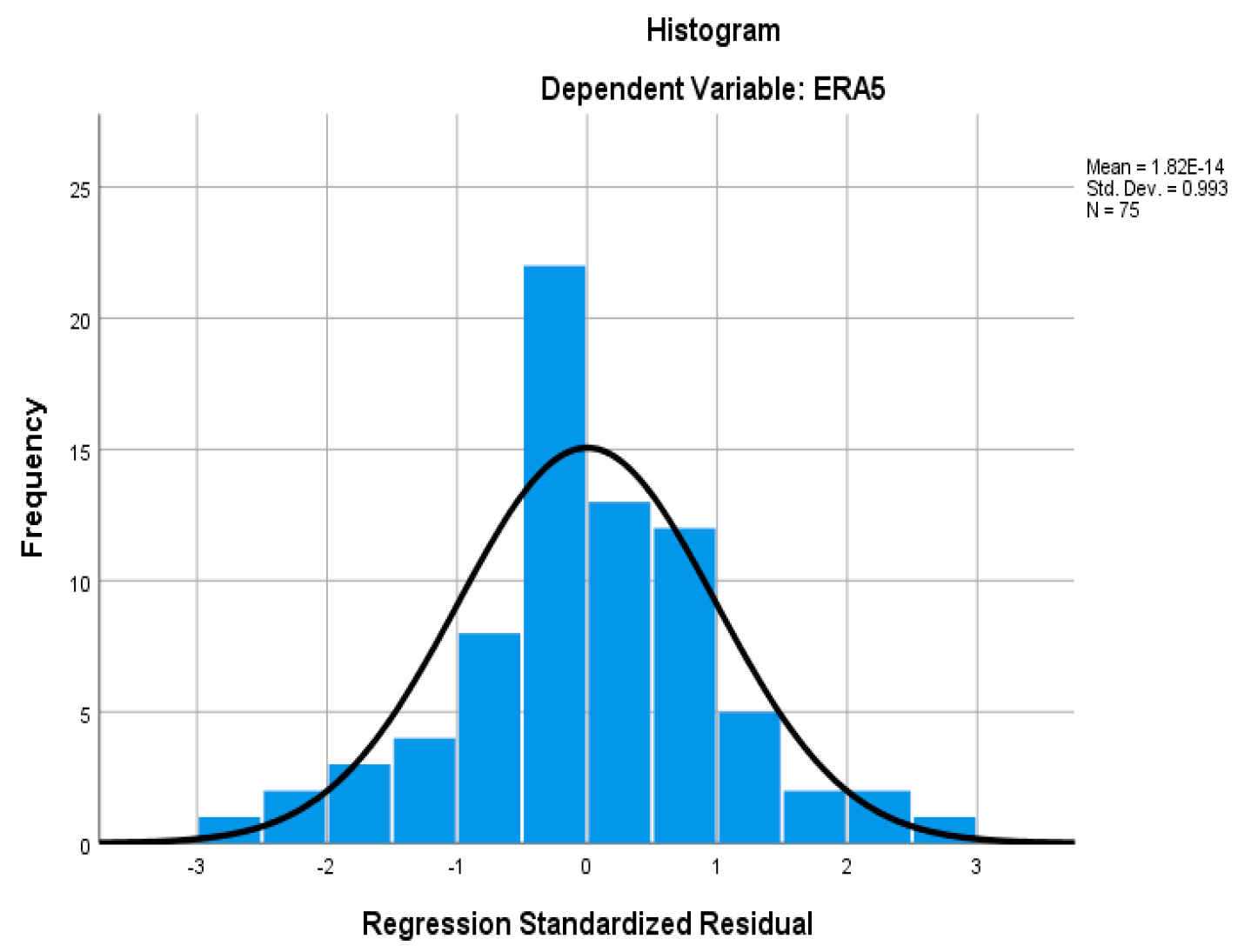
The histogram graph above shows that the CMIP6 model outputs are normal distribution for the future trends (2030 - 2100). The histogram graph was performed as one of the assumptions that should be checked before building forecasting model to ascertain model normality and linearity. It is important to evaluate the goodness-of-fit and the statistical significance of the estimated SST model outputs of the constructed regression models; the techniques commonly used to verify the goodness-of-fit of regression models are the hypothesis testing, R-squared and analysis of the residuals. In this case, the histogram is skewed towards positive correlations suggesting that the CMIP6 model simulation and the observed are likely to lead to a skill teleconnection between the SST anomalies and West African rainfall climatology.
Figure 13.
Standardized residual plot.
Figure 13.
Standardized residual plot.
The output from the CMIP6 model outputs performed for all the outputs showed a smooth trend for the future scenarios (2015-2100). The regression line is a trend line we use to model a linear trend that we see in a scatterplot but realize that some data will show a relationship that isn't necessarily linear. Such was the output obtained for the historical model comparisons with the ERA5 SST data (1940 - 2014).
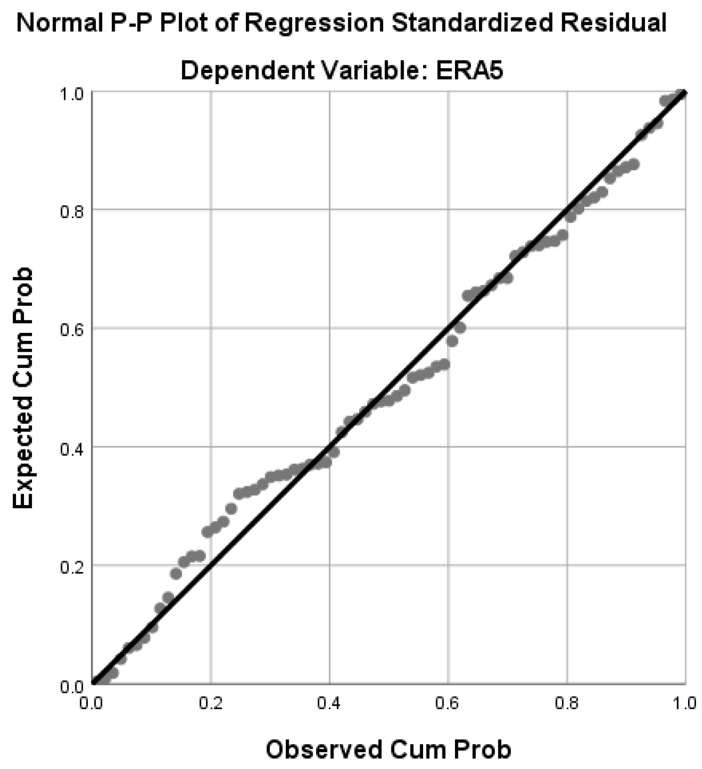
The P-P plot compares the observed cumulative distribution function (CDF) of the standardized residual to the expected CDF of the normal distribution. The normal probability plot indicates whether the residuals follow a normal distribution, in which case the points will follow a straight line. Often some moderate scatters as shown below are often expected even with normal data, it shows that some of the model outputs performed well in some periods within the climatic years of study. In this study, P-P (probability–probability) plot was employed as a visualization plot of the CDFs and the two distributions (empirical and theoretical) against each other.
The results however showed that the CMIP6 multi-model ensemble mean values (and CVs) for the six indices have similar magnitude and pattern of variations as reanalyzes over the Gulf of Guinea, except the MCM-UA (USA).
5. Summary and Conclusion
The study evaluated the performance of bias corrected GCM-CMIP6 models in stimulating the historical and future projection of SST over the Gulf of Guinea involving ACCESS-CM2 (Australia) CAMS-CSM1-0 (ChinaCanESM5-CanOE (Canada), CMCC-ESM2 (Italy) HadGEM3-GC31-LL (UK) EC-Earth3-CC (Europe) MCM-UA-1-0 (USA) MPI-ESM1-2-LR (Germany) while ERA5 reanalysis data was used as the observed/historical dat for validation of the models. Given the fact that GCM spatial resolution are often too coarse, the bias-corrected dataset was developed using Empirical Quantile Mapping (EQM) for the historic (1940–2014) and projected (2015–2100) to get reliable projections at the regional and local scale. The CMIP6 GCM model projection further revealed that ACCESS-CM2 CAMS-CSM1-0, CanESM5 Canada, CMCC-ESM2 and MCM -UA performed better in reproducing the observed SST climatology. The future SST projection by the models indicate that on the average SST will warm by 1.03oC between 2030 and 2040 and a projection of 35oC by 20100 against the historical observation of 30o simulated by the models between 1970 and 2014 for the high warming and 21o for the Western Sahel. The model evaluation using coefficient of regression indicates that the all models namely ACEES, CAMS-CSM. CAN-ESM, CMCC, MUM and MP-ESM have R values of 0.10, 0.01, 0.06. 0.09, 0.10 and 0.013 respectively. The weakest correlation is CAMS-CSM model 0.01 while the strongest correlation emanates from MUM-UA with 0.13 which further demonstrates the fidelity of the models in reproducing the observed SST climatology of the Guinean coast.
In view of the forgoing, the study concludes that the 8 CMIP6 models that were examined both underestimated and overestimated SST over the GOG relative to the ERA5 reanalysis dataset, which was evident over the GOG. The cold bias is mainly focused over the Western Sahel which is most obvious during the cold season while the warming bias dominates the Guinean coast. The models were generally successful in representing the spatial variability of climatological mean sea surface temperature. One of the implications of the projected future SST warming is that it will drives changes in the meridional and zonal SST gradients with deleterious impact on the local climate and beyond and the location of the Intertropical Convergence Zone (ITCZ) which is a function of the underlying SST and the equatorial meridional SST gradients. In addition, Small spatial differences in SST warming can also trigger changes in winds and hence rainfall strength and distribution in the future. Finally, the study concludes that the projected increase in future SST over the GOG will be higher in the Far period end than the Near-term climate. Overall, the bias corrected CMIP6 projections can be used for multiple assessments related to climate and hydrological impact studies and for the development of mitigation measures under a warming climate.
The authors are grateful to the two anonymous reviewers for their time and effort in reviewing this work. These suggestions have made this work much stronger.
Author Contributions
The first author conducted the entire research including, simulation, analysis, and preparation of the draft manuscript while the second author reviewed the manuscript and supervised the researcher in his Lab as Postdoc Adviser in the school of Natural resources, university of Missouri Columbia.
Funding
This research was funded by the federal Government of Nigeria through Tertiary Education Trust Fund (Tetfund) and the Dr Tony research group in the school of natural resources, University of Missouri Columbia as postdoctoral research award granted to Oye Ideki
Competing Interests
The authors declare that there is no competing interest.
References
- Adeniye. M.O (2017) Modeling the impact of changes in Atlantic sea surface temperature on the climate of West Africa Meteorol Atmos Phys 129:187.
- Ahmed, K., Shahid, S., Sachindra, D.A., Nawaz, N., Chung, E.S.(2019) : Fidelity assessment of general circulation model simulated precipitation and temperature over Pakistan using a feature selection method. J. Hydrol. [CrossRef]
- Akinsanola,A.A.A, Ajayi,V.O; Adejare,A.T; Adeyemei, O.E; Gbode,E; Ogunjobi,R.O, Nikulin,G and Abolade,A.T (2018): Evaluation of rainfall simulations over West Africa in a dynamically downscaled CMIP5 global circulation models. Journal of theoretical and applied climatology. 132:437-45.
- Breugem, W. P., Hazeleger, W. and Haarsma, R. J. (2006). Multimodal study of tropical Atlantic variability and change. Geophysical Research Letters, 33.
- Brown, J.N; Langlais.C and Gupta, A.S (2015) Projected Sea surface temperature changes in the equatorial pacific relative to the warm pool; edge. Elsevier journal of Sea Research II Vol.13. 47-58.
- 6. Burls, N. J., Reason, C. J. C., Penven, P. and Philander, S. G. (2012). Energetics of the tropical Atlantic zonal mode. Journal of Climate, 25, 7442–7466. [CrossRef]
- 7. Chokkavarapu, N., Mandla, V.R.: Comparative study of GCMs, RCMs, downscaling and hydrological models: a review toward future climate change impact estimation. SN Appl. Sci. 1, 1698 (2019). [CrossRef]
- Christensen JH, Hewitson B, Busuioc A, Chen A, Gao X, Held I, Jones I, Kolli RK, Kwon WT, Laprise R, Magan˜a Rueda V, Mearns L, Mene´ndez CG, Ra¨isa¨nen J, Rinke A, Sarr A, Whetton P (2007) Regional climate projections. In: Solomon S, Qin D, Manning M, Chen Z, Marquis M, Averyt KB, Tignor M, Miller HL et al (eds) Climate change 2007: the physical science basis. Contribution of Working Group I to the Fourth Assessment Report of the Intergovernmental Panel on Climate Change. Cambridge University Press, Cambridge.
- Christensen JH, Kumar KK, Aldrian E, An S-I, Cavalcanti IFA, de Castro M, Dong W, Goswami P, Hall A, Kanyanga JK, Kitoh A, Kossin J, Lau N-C, Renwick J, Stephenson DB, Xie S-P, Zhou T (2013) Climate phenomena and their relevance for future regional climate change supplementary material. In: Stocker TF, Qin D, Plattner G-K, Tignor M, Allen SK, Boschung J, Nauels A, XiaY, Bex V, Midgley PM (eds) Climate change 2013: the physical science basis. Contribution of Working Group I to the Fifth Assessment Report of the Intergovernmental Panel on Climate Change.
- 10. Christensen, J. H., Boberg, F., Christensen, O. B. & Lucas-Picher, P. On the need for bias correction of regional climate change projections of temperature and precipitation. Geophys. Res. Lett. 35(20) (2008). [CrossRef]
- Cook K.H, Vizy E.K (2006) Coupled model simulations of the West African monsoon system: twentieth-and twenty-first-century simulations. J Clim 19(15):3681–3703.
- 12. Gidden MJ, et al.(2019) Global emissions pathways under different socioeconomic scenarios for use in CMIP6: A dataset of harmonized emissions trajectories through the end of the century. Geosci. Model Dev.12:1443–1475. [CrossRef]
- Giorgi, F. and Gutowski, W. J.(2015) Regional Dynamical Downscaling and the CORDEX Initiative. Annu. Rev. Environ. Resources 40, 467–490. [CrossRef]
- Iloeje N.P. (1981). A New Geography of Nigeria. Longman: Great Britain; 259. Janicot S, H.
- IPCC (2019) Ocean and climate change: New challenges. Focus on 5 key themes of the IPCC Special Report on the Ocean and Cryosphere.
- IPCC, 2022: Climate Change 2022: Impacts, Adaptation and Vulnerability. Contribution of Working Group II to the Sixth Assessment Report of the Intergovernmental Panel on Climate Change [H.-O. Pörtner, D.C. Roberts, M. Tignor, E.S. Poloczanska, K. Mintenbeck, A. Alegría, M. Craig, S. Langsdorf, S. Löschke, V. Möller, A. Okem, B. Rama (eds.)]. Cambridge University Press. Cambridge University Press, Cambridge, UK and New York, NY, USA, 3056 pp.
- Jose,P.M and Dwarakish,G.S (2021) Bias correction and trend analysis of temperature data by a high resolution CMIP6 model over a tropical river Basin . Asia-Pacifoic journal of Atmospheric sciences. Springer.
- Li, Z; Liu T, Huang Y, Peng J and Ling Y.(2022) Evaluation of the CMIP6 Precipitation simulations over global land. Earth’s Future 10(8):1–21.
- Lübbecke, J.F; Belen Fonseca, B.R; Richter. I; Martín-Rey. M; Losada. T, Polo.I; Keenlyside, N.S (2018) Equatorial Atlantic variability – modes, mechanisms, and global teleconnections. Wires Wiley journal of Interdisciplinary reviews.
- Ojo O. 1977. The Climates of West Africa. Heinemann: London; 219.
- Palmer.P.I, Wainwright, C.M, Dong ,B. Maidment, R.I, Wheeler ,K.G , Gedney. N , Hickman, J.E; Madani. N; Folwell.S.S ; Abdo.G; Allan, R.P; Emily Black,C.L , Feng, L; Gudoshava ,M; 14, Haines, K ; Huntingford, C Kilavi,M; Lunt. M.F Shaaban, A; Turner, A.G (2023) Drivers and impacts of Eastern African rainfall variability. Nature Reviews; Earth and Environment. Vol.4; 254-27.
- Raper, S.C.B. and Cubasch, U (1996) Emulation of the results from a coupled general circulation model using a simple climate model. Geophys. Res. Lett. 1996, 23, 1107–1110.
- 23. Roberts C.D, Palmer M.D, Mcneall D and Collins M. (2015). Quantifying the likelihood of a continued hiatus in global warming. Nature Climate Change 5: 337-. [CrossRef]
- Rodwell,D.P (2013) Stimulating SST teleconnections to Africa: What is the state of the Art. Met Office, Hadley Center, Fritz Roy Exeter, United Kingdom.
- Seager R, Naik N, Vogel L (2012) Does global warming cause intensified interannual hydroclimate variability? J Clim 25:3355–3372. [CrossRef]
- Siongco AC, Hohenegger C, Stevens B (2015) The Atlantic ITCZ bias in CMIP5 models. Clim Dyn 45(5–6):11.
- Sung, H.M.; Kim, J.; Lee, J.-H.; Shim, S.; Boo, K.-O.; Ha, J.-C.; Kim, Y.-H (2021) Future Changes in the Global and Regional Sea Level Rise and Sea Surface Temperature Based on CMIP6 Models. Atmosphere 12, 90. [CrossRef]
- 28. Trasher, B., Maurer, E. P., McKellar, C. and Dufy, P. B. Technical Note: Bias correcting climate model simulated daily temperature extremes with quantile mapping. Hydrol. Earth Syst. Sci. 16, 3309–3314 (2012). 35. [CrossRef]
- UNFCCC (2021) State of the climate: Extreme events and major impacts. Bonn Germany.
- Vizy, E.K and Cook, K.H (2001) Mechanism by which Gulf of Guinea and Eastern North Atlantic Sea surface temperature Anomalies can influence African Rainfall. Journal of Climate, American Meteorological Society. Vol.14.
- White, R. H. and Toumi, R. (2013) The limitations of bias correcting regional climate model inputs. Geophys. Res. Lett. 40, 2907–2912 (2013). 40. [CrossRef]
- Wijffels S, Roemmich D, Monselesan D and Church J, Gilson J.( 2016). Ocean temperatures chronicle the ongoing warming of Earth. Nature Climate Change 6: 116-118 warming. Nature Climate Change 5: 337-342. [CrossRef]
|
Disclaimer/Publisher’s Note: The statements, opinions and data contained in all publications are solely those of the individual author(s) and contributor(s) and not of MDPI and/or the editor(s). MDPI and/or the editor(s) disclaim responsibility for any injury to people or property resulting from any ideas, methods, instructions or products referred to in the content. |
© 2023 by the authors. Licensee MDPI, Basel, Switzerland. This article is an open access article distributed under the terms and conditions of the Creative Commons Attribution (CC BY) license (http://creativecommons.org/licenses/by/4.0/).
