Preprint
Article

Navigating Choppy Waters: Interplay between Financial Stress and Commodity Market Indices

Altmetrics

Downloads

111

Views

50

Comments

0

A peer-reviewed article of this preprint also exists.

This version is not peer-reviewed

Submitted:

21 November 2023

Posted:

23 November 2023

You are already at the latest version

Alerts
Abstract
Financial stress can have significant implications for individuals, businesses, asset prices and the economy as a whole. This study examines the nonlinear structure and dynamic changes in the multifractal behavior of cross-correlation between the financial stress index (FSI) and four well-known commodity indices, namely Commodity Research Bureau Index (CRBI), Baltic Dry Index (BDI), London Metal Index (LME) and Brent Oil prices (BROIL), using multifractal detrended cross correlation analysis (MFDCCA). For analysis, we utilized daily values of FSI and commodity index prices from 16th June 2016 to 9th July 2023. The following are the most important empirical findings: (I) All of the chosen commodity market indices show cross correlations with the FSI and have notable multifractal characteristics. (II) The presence of power law cross-correlation implies that a noteworthy shift in FSI is likely to coincide with a considerable shift in the commodity indices. (III) The multifractal cross-correlation is highest between FSI and Brent Oil (BROIL) and lowest with LME. (IV) The rolling windows analysis reveals a varying degree of persistency between FSI and commodity markets. The findings of this study have a number of important implications for commodity market investors and policymakers.
Keywords: 
Subject: Business, Economics and Management  -   Finance

1. Introduction

Financial stress can have significant implications for individuals, business, and economies. It can harm individuals’ physical and mental health, relationships and work, leading to substance abuse and even in some cases to suicide [1,2,3,4,5,6]. It refers to a discomfort or strain that individuals or entities face due to taking on a high risk or increasing the gap between their obligations and available means [7]. Financial stress also leads to an increased crime rate and damages the social fabric of society [8,9]. It is well documented that financial stress not only impacts on business operations (i.e., staff lay-off, production cut-backs), but also impacts on trading and investment strategies [10,11,12]. To avoid extreme losses, investors become reluctant to trade and withdraw their investment during periods of high stress and uncertainty [13]. Increased financial stress leads to lower business activity and slows down economic expansion [14,15]. The situation can also precede a trust deficit in the financial system [15,16], which can make it difficult for businesses to borrow and invest funds. It also adversely affects the economy, and can lead to a significant decline in consumer spending and investment, which slows down the rhythm of economic growth. It spreads among developed economies through financial, trade and economic channels, and may extend to emerging economies [17,18,19,20,21], affecting macroeconomic indicators [16,21,22] and causing currency market crises [23,24]. Financial stress can be connected to financial instability through entities’ failures [25]. For instance, if the banking system is under stress, banks may be more likely to fail [14,20,26,27]. The situation of loss of trust in the financial system followed by a rise in inflation can make it difficult for borrowers and businesses to access funding [28]. It increases poverty and inequalities, disrupting trade and capital flows and having long-term negative effects on the global economic system. It reduces economic growth, increases unemployment and causes volatility in stock [29] and commodity markets [30].
A growing body of research shows that financial stress affects the performance of stock, cryptocurrency, forex, energy, commodities, and other markets, as well as managerial decisions. Its ups and downs impact asset prices, such as stocks, bonds, gold, oil and cryptocurrencies [31,32,33,34]. Past research shows that financial stress affects different classes of economies and main markets, circulating within countries as well as expanding to different economic sectors. The literature reports its spread to various markets and expansion, mainly in financial markets, showing a connection with the foreign exchange market [16,23,35], banking crises [24,27,36] oscillations in equity and bond markets [31,37,38,39,40,41] monetary policy [42,43] and the crypto market [44]. In the commodities a great amount of research has focused on energy related commodities, [45,46,47,48] revealing a meaningful association with energy markets. There is a dynamic relation with the FSI (Financial Stress Index) and linkages between commodity spot and futures prices through channels of inflation, the demand supply gap and investors searching for a safe haven to mitigate portfolio risk [45,49,50,51,52].
Researchers and academics have recently focused more on the commodity market, looking at the relationship between the commodity market and financial stress. Investors in commodities take into account the financial stress that is prevalent in the global economy due to any cause. A large number of studies have focused on the linkage between financial stress and different asset categories and market indices as well as different categories of commodity market future prices such as agriculture, metals and energy [53]. Ordinarily, commodities are far from being a uniform asset class and show a wide range of characteristics. While some commodities, like industrial and precious metals, may be inventoried, others, including energy and livestock products, can only be stored for shorter periods at extremely high costs. In addition, commodities’ return distributions differ from conventional assets. Commodity returns typically have positive skews, which reduces downside risk but also produces fat tails [51,54]. Energy commodities show volatile behavior in correlation with financial markets and in contango times dependency on their past returns condition capitalizes to prices rising more and falling prices keep falling [55]. In the response of GFC 2008, financialization of commodity markets has enhanced their correlations and diminished the heterogeneity of several key commodities’ returns, especially indexed commodities [56]. It is a fact that commodity prices over the decades underwent booms and slumps. Such changes in commodity prices can have disastrous economic and social consequences because many developing nations depend heavily on commodities as their primary source of income [22,57]. Its contagion has not been explored with the composite indices of commodities like CRBI, BDI, LME and BROIL. Financial stress attracted more attention after the recession and inflation episodes in response to the recent catastrophic occurrences of the global financial crises 2007-09, European credit risk crises 2010-12, covid-19 pandemic recession and recovery period shocks [58,59,60], and the Russian invasion of Ukraine in 2022. There are numerous causes of financial stress but the most important are natural disasters, geopolitical tensions [61,62,63], structural vulnerabilities [34], economic shocks, and corporate failures [64].
This work differs from previous studies in at least three ways. First, using a Fractal Market Hypothesis framework, it looks at the cross-correlations between the FSI and four commodity market indices, covering the prices of many different commodity returns: the BDI, LME, BROIL and CRBI. The dynamics of a wide range of significant commodity indexes, which are still subject to scholarly attention, are examined in this paper. Second, it is unknown how the cross-correlation between the commodity markets and the FSI exhibits multifractal behavior. To be more precise, a multifractal measure can be understood broadly mathematically as a fractal measure defined on a fractal domain or set, where multifractality results from the interaction of two families of singularities [65]. We use the econophysics based MFDCCA, which was first presented by [66], to look into cross correlations between the commodity market indices and the FSI. When it comes to finding nonlinear relationships, which linear approaches frequently fail to reveal, MFDCCA is a better option [67,68]. Thirdly, by applying the rolling windows approach, this study, grounded on the perspective of the commodity market, provides a more thorough understanding of that market’s dynamics over time. In particular, the power law cross-correlation between fluctuations in FSI and commodity prices indicates that, rather than the other way around, a major change in the FSI was likely caused by a big shift in commodity market prices. Different degrees of multifractality are discovered, with the FSI BROIL showing the highest levels of multifractal cross-correlation and the FSI and LME showing the lowest. Furthermore, the commodity markets show more dependable persistent cross-correlations for small swings than for major ones. These results will enable regulators and institutional investors to develop efficient investment plans and policies while taking the FSI’s fluctuations and alerts into account. To maintain financial stability amid these challenges, policy makers, global economic forums and regulatory bodies need to adopt a coordinated, comprehensive approach. They must take precautionary measures such as strengthening financial oversight, for instance FSI, and responding promptly to its alerts. Larger buffers should be formed, by reducing incentives for higher risk taking and increasing capital and liquidity requirements, as stated by Cardarelli, Elekdag and Lall [28]. Financial stability enables the efficient propagation of financial means within a society, by timely and effective allocation of funds and initiating profitable investment [69].

2. Materials and Methods

We applied the MFDCCA method to explore cross-correlations between FSI and four commodity market composite indices. The daily datasets range from 16th June 2016 to 9th July 2023. The first dataset consists of daily values of FISI retrieved from the official website of Office of Financial Research (www.financialreseach.gov). The FSI was developed by Office of Financial Research (OFR) to detect the threat of financial crises in advance [19]. The index utilizes a unique and flexible methodology using daily data from global financial markets. Analysis of the FSI index covers the period from 2000 to 2018. The paper highlights that the OFR_FSI performs well in identifying systemic financial stress, as demonstrated through a logistic regression framework and the use of government intervention dates as proxies for stress events. Additionally, alerts of increased financial stress, as indicated by the OFR FSI, can help predict decreases in economic activity, as shown by a Granger causality analysis comparing the index with the Chicago Fed National Activity Index. It is used to measure and assess the level of strains and risks in a financial system or economy. It provides signals in advance in order to address adverse events and helps in developing appropriate responses. [57] argues it is typically positive when the stress level is above average and negative when stress is below average. Additional classifications included in the OFR_FSI are credit, fundings, equity valuation, safe assets, and volatility. It is typically designed by compounding a variety of variables that emulate several facets of the financial system, such as credit spreads, market volatility, bank funding and liquidity. The FSIs are found to be useful in predicting economic and financial outcomes, improving forecasts, and identifying high-stress episodes. They also highlight the non-linear effects of financial stress on several variables. Overall, FSIs play a crucial role in monitoring and managing financial stability and can assist policymakers and researchers in making informed decisions [70].
The other data set is commodity market indices including the CRBI, BDI, LME and BROIL. The daily prices (USD) of commodity indices are collected from DataStream. Global commodity market indices are essential for the global economy because they provide useful data, benchmarks and clues with an impact on numerous types of economic activities around the world. This study focuses mainly on the four global commodity indices. The particulars of the commodity data set, their coverage and weights are provided in Table 1. CRBI was considered as a measure that comprehensively tracks movements in all economic sectors [71]. The effectiveness of a commodity price index as a precursor to inflation is investigated by multiple studies [71,72,73]. Since 1956, the CRBI has kept track of a broad index of commodity prices. Furthermore, we utilized the BDI index, considered as a world import indicator [74] to gauge economic activity. It is an effective predictor of commodity, stock returns and economic activity [75,76] major currencies’ exchange rates [77], industrial production and financial asset prices [78]. The index has undergone many revisions since its inception to preserve its empirical relevance. The most recent revision, which came into effect in 2005, comprises 19 commodities and assigns higher weights to different commodities based on their importance. For the execution of MFDCCA, commodity datasets are matched with FSI after performing the data cleaning process. We removed extreme inorganic observations from the FSI for the sake of brevity, as these showed abrupt unnatural negative and positive changes in daily stress changes. We converted the indices into daily changes to determine the cross-correlation between the FSI and certain chosen commodities.
Figure 1 plots daily index values for FSI, CRBI, BDI, LME and BROIL in subcategories from A to E respectively. Panel A represents the daily values of FSI and plots a graph line for the sample period from 16th July 2016 to 9th July 2023. From July 2016 to February 2020, FSI remained below the average line, except for a single spike in 2018 for a shorter time span. This established that global economies were recovering after the global financial crises of 2008. The policies and structures incorporated to tackle such crises and policies strengthen the confidence of investors and the business community to participate in economic activities and make investment. In the interim, decision-makers focused on developing policies and precautionary steps to avert crises of this nature. The period from 2012 to 2017 is particularly captivating because of the positive bubble in the US currency and the negative bubble in the oil market [79]. Moreover, a short span stress spike cropped up during the last quarter of 2018 due to the US-China trade conflict [44]. Throughout the sample period, the largest stress spikes were observed during the Covid-19 period from the end of the first quarter of 2020 to the end of the second quarter of 2022. On 11th March 2020, the WHO declared Covid-19 as a global pandemic [80], and in April 2020 suggested lockdown. Lockdown caused a sudden rise in financial stress from the beginning of the second quarter of 2020 [81]. With the relaxation of lockdown, financial stress decreased below the average line and financial conditions remained stable from the end of the second quarter of 2020 through the last quarter of 2021 as seen in the graph. The FSI graph line again exhibited a rising trend from February 2022 because of the Ukraine-Russia war [82], Russia invaded Ukraine on 24th February 2022. The stress time span is longer during this period, with the FSI line remaining above the average line from February 2022 to December 2022. For the remaining period till July 2023, the FSI graph remained stable on the average line.
Panel B shows the CRBI daily values graph on average remains stable with minor variations from June 2016 to March 2020, with a sharp decline from April 2020 to May 2020 and reaching its lowest point in the sample period during the Covid-19 lockdown period. It rises gradually and then sharply from December 2021. Commodity prices have increased significantly as lockdowns around the world have decreased and economies return to a more normal trend. In response to the market recovery period after Covid-19, the CRBI graph touched its highest point in February and March 2022. However, from July 2022 the CRBI graph line shows a gradual declining phase and a sharp decline in March 2022 because of the Russia-Ukraine war. The index line shows that since the start of 2023 commodity prices have dropped 13.02 points, or 4.3%. Compared to pre Covid-19, prices remained elevated till July 2023. Commodity prices will remain high in 2023 due to high energy costs, shortages of agricultural supply brought about by the Russia-Ukraine war, and unfavorable weather patterns.
Panel C of Figure 1 shows the daily values of the BDI and shows a downward trend as 2016 got underway amid worries about China’s slowing economy, which had an impact on the demand for commodities globally. Lower shipping costs and a drop in the BDI were caused by decreased Chinese imports. Due to an oversupply of ships, the index continued to fall in December 2016 and did so into the first quarter of 2017. As long as commodity prices were high, economies started to increase again in March 2017. By May, it had reached its peak and was therefore quite stable. The BDI’s upward trajectory was disrupted once more in December 2017 as trade tensions between the US and China increased concerns about world trade. It was further affected from March 2018 to May 2018 due to the Iranian sanctions. Due to trade concerns, the downward trend persisted until January 2019. The index began to rise once again in February 2019 as trade tensions between the US and China briefly subsided. Downward trends through January 2020 were brought on by Brazilian iron ore extraction and increased shipping costs. The BDI showed very minor variations at the end of the year in December 2019. The COVID-19 pandemic caused a large fall in shipping demand from February 2020, which caused the BDI to decline sharply. From April through June 2020, the BDI reached its lowest point of the year. After the first phase of the COVID-19 crisis, lockdowns were relaxed, and an inclining trend started. The multiple COVID-10 pandemic events, lockdowns, and corresponding seasonal changes all had an ongoing impact on BDI. It began to rise as the economic recovery got underway, but was still below pre-pandemic levels. As global trade and commodity demand started to recover in February 2021, the BDI kept moving upward. Continuous supply chain disruptions led to changes in shipping costs in May 2021. Because of these factors, the BDI reached its peak in October 2021. In 2021, there was a significant demand for several important commodities, including grain, iron ore, and coal. Shipping costs rose significantly because of China’s high demand for iron ore. The demand for large quantities of commodities was also influenced by the recovery of the global construction sector and the demand for energy resources. Industrial raw material caused the index to maintain its pre-pandemic level after the boom until January 2022. In February 2022, there were many noticeable seasonal variations, but in March, the Russia-Ukraine war’s impact on the closure of shipping lanes caused a spike in shipping expenses. Due to fewer coal imports to Europe and China’s slow economic recovery, the BDI showed a severe downward trend from January to February 2023. From March onward, the index returned to its usual threshold, but in the second half of June started to decline again and fell below 1,000 points, 13% down in July for the first time in a month due to the diminished shipment of coal and Iron.
Panel D plots the graph line of LME, interestingly showing a similar pattern from the beginning of the sample period, during the US-China trade conflict in 2018, and the Covid-19 crises in 2020, as well as a similar pattern after the covid-19 recovery period. It was different during the Ukraine Russia war and showed a sharp declining trend, remaining unstable during the period as compared to CRBI.
Finally, Panel E shows the BROIL throughout the period of our study. The first notable downward trend is from April through June 2016, due to the oversupply of U.S crude oil from 384000 b/d to 9.2 million b/d, this dent being created by supply pressure on oil prices [83]. This increased the price differential between Brent and WTI while decreasing the demand for Brent crude oil, which serves as the benchmark for the majority of global crude oil trade. Furthermore, in May 2017, OPEC, and its collaborators, including Russia, agreed to extend their production cuts through March 2018. While this was projected to stabilize prices, it also highlighted the ongoing challenges in rebalancing the market. Despite the November 2018 sanctions, the US granted exceptions to eight countries, allowing them to keep importing oil from Iran. This allayed the supply shortfall worries that had raised prices earlier in the year. Oil production in Saudi Arabia, Russia, and the US all reached new highs, outpacing the rate of increase in demand from November through December 2018. The BROIL started an inclining trend due to the supply demand gap and remained stable till February 2020 before the Covid-19 outbreak. The Brent oil price decreased to the lowest ever as the WHO declared the Covid-19 lockdown in March 2020, remaining down throughout Covid-19 because of the crunch in global oil demand. From May 2020 onwards, after the easing of Covid lockdowns, BROIL started a gradual increase, experiencing a recovery period after the longest recession period after Covid-19. March 2022 shows increasing spikes in response to the Ukraine-Russia war because Russia is the second largest oil producer in the world. There was fear of the widening supply demand gap throughout the world. Brent prices gradually returned to their normal prices after June 2022 and remain stable thereafter.

2.1. Multifractal Detrended Cross Correlation Analysis (MFDCCA)

Zhou [66] states that the following phases summarize the MFDCCA algorithm:
With N denoting the length of the time series, we can calculate the remaining component for the commodity market composite indices and the FSI by taking into account the two times series ( x i ) and ( y i ) of an equal length. X i and Y i signal profiles are initially put together as follows.
X i = i = 1 j   x i   x ¯ , i = 1 , 2 , 3 . , N ,
Y i = i = 1 j   y t   y ¯ , i = 1 , 2 , 3 . , N ,
Where the mean values of ( x i ) and ( y i ) , respectively, are represented by x ¯ and y ¯ . The profiles X i and Y i are divided into N s = i n t N s boxes of the same length s . Even so, as t N might not always be a non-multiple of s , the reserve series of the profile is maintained using the same technique, yielding 2 N s without overlapping splits being gained.
Third, we investigate each portion’s local pattern X v   ( i ) and   Y v   ( i ) of each segment and probe the variance for each v = 1 ,   2 ,   ,   2 N s as:
F 2 s , v = 1 s i = 1 s X   v 1   s + i X v   ( i )   .   Y   v 1   s + i Y v ( i )
for each divide v = 1 ,   2 ,   . . ,   N s and
F 2 s , v = 1 s j = 1 s   X N v N s s + i X v ( i ) . Y N v N s s + i Y v ( i )
for v = N s   ,     .   . ,   2 N s .
Fourth, we use the following equation to compute the q th sequence variations function.
F q   s = 1 2 N s v = 1 2 N s F 2   s ,   v q / 2 1 / q
For any q 0 , while for q = 0 it is shown as:
F 0 s = e x p 1 4 N s v = 1 2 N s l n F 2 s , v
Here, with F q s being an increasing function of s, we retrieve the conventional DCCA at q = 2 .
Finally, in order to identify the multi-scaling pattern of the fluctuation, we investigate the log - log plots of F q s against s for each q.
F q s ~ s H x y q
In this case, the scaling exponent H x y q denotes the power-law relationship between two non-linear time series, which shows the magnitude of F q s as a function of the scale step s. When there is similarity between the two time series of ( x i ) and ( y i ) , MFDCCA indicates a distinctive case of MFDFA.
The long-range cross-correlations of two time series coexisting simultaneously can be characterized using multifractal detrended cross-correlation analysis (MFDCCA) [84]. If a normal stationary time series occurs, the Generalized Hurst Exponent at H x y 2 , is comparable to the conventional Hurst exponent h [85]. Moreover, H x y 2 = 0.5 shows that there is no cross-correlation between the two series. On the other hand, the presence of cross-correlation between the two time series is persistent at H x y   2 > 0.5 , indicating positive correlation between the two series. The cross-correlation shows anti-persistence behavior and inverse association, or -ve cross-correlations, where H x y 2 < 0.5 2).
According to [86], the multifractality degree ∆H is defined as follows:
H = H m a x ( q ) H m i n ( q )
The H reflects the strength of multifractality. A larger value of H denotes the strongest level of multifractality. Furthermore, with further cross-correlations, the corresponding values of H x y q can show the degree of multifractality. Through the Legendre transform, the following can be acquired to calculate the degree of multifractality.
α = H q + q . H x y ( q )
Consequently, the singularity spectrum f α can be constructed as follows:
f α = q ( α H x y q ) + 1

2.2. Multifractal Indices

2.2.1. The degree of multifractality

The multifractal strength can be estimated by the following spectrum width α .
α = α m a x α m i n
A larger multifractality is represented by a broader multifractal spectrum.

2.2.2. Degree of asymmetry (AI)

The asymmetric intensity likewise represented as the skewness of f ( α ) spectrum, can be acquired as under:
A I = α m a x α 0 α 0 α m i n
The fractal exponent, represented by the power law exponent 𝛼, is the fractal onset time, quantifies the strength of time-clustering, and delimits the lower bound of significant scaling behavior in the variables [87]. However, the value of α is represented by the α 0 , if f ( α ) is at its maximum. It has three different shapes associated with the values of A, which indicate the asymmetry position as positive-skewed ( A I > 1 ) , symmetric ( A I = 1 ) , or negative-skewed ( 0 < A I < 1 ) , according to Freitas, et al. [88]. The extreme values of the singularity exponent are represented by the right end point, α m a x and the left end point, α m a x which correspond to the minimum and maximum fluctuations of the signal, respectively.

2.2.3. Singularity parameters

The singularity ratio C is utilized, and it can be computed as the ratio of f l e f t ( α ) and f r i g h t ( α ) , evaluated in relation to the maximum fractal dimension f m a x [ α ( q = 0 ) ] . The singularity ratio index C can be interpreted as a direct measure of truncation, with C > 1 denoting the left side of truncation and C < 1 denoting the right side. The formula below can be used to calculate the strength in the singularities, which is represented by the proportional ratio f ( α ) between the widths of the left and right sides.
C = f L ( α ) f R ( α ) = 1 f L m i n ( α ) 1 f R m a x ( α )
According to [89], the intensity of the multifractal spectrum and the singularity strength α have an inverse relationship. Furthermore, higher values of h indicate smoother variations because of the weakening of the singularity.

2.2.4. The Hurst index (H)

According to [90], the generalized Hurst exponent h ( q = 2 ) is used to determine the Hurst index ( H ) at second-order. Furthermore, [91] described a method of classifying different types of processes by identifying the characteristics of 1 / f β noises, which have a Fourier power spectrum scaling element β . Nevertheless, the slope of a linear trend is used to calculate β . In a similar vein, the trend can be either 1 < β < 1 for f G n , or 1 < β < 3 . Furthermore, [88] claimed that the relationship β = 2 + τ ( 2 ) can be used to estimate β . Long-range dependence (LRD) between the non-linear data series is represented by the values of H , which vary from 0.5 to 1. The closer a value is to 1, the higher the periodicity. On the other hand,   H values close to zero denote white noise, while H = 0.5 denotes uncorrelated data.

3. Empirical Results

3.1. Descriptive Statistics

Table 2 describes the summary statistics of the FSI and Commodity market indices. The mean of the FSI is -0.0012, while for commodity indices LME shows the highest mean value followed by BDI, CRBI and BROIL. BDI exhibits the highest range in all commodity series followed by LME, CRBI BROIL and FSI. Range depicts the spread between minimum and maximum returns from the sample time span under study. BDI showed more volatile behavior (S.D = 0.54) followed by LME, CRBI, BROIL, and FSI exhibited the least volatile behavior (S.D = 0.270). FSI is right skewed contrary to the BROIL which is left skewed. CRBI is moderately skewed while the BDI and LME are approximately skewed. The Kurtosis scores determined that aside from LME all the other series exhibit heavy tails as their kurtosis score is highly positive and more than three. The verification of high kurtosis levels is a common result, meaning the presence of fat tails, a feature related with the Fractal Market Hypothesis. The Jarque-Bera (JB) test of goodness of fit was applied to diagnose the normality of the data series. The findings for all variables are significant at 1% significance. The null hypothesis of the JB test “data is normally distributed”, in the light of the above results, is rejected. The Augmented Dicky-Fuller (ADF) test was applied to assess the stationarity of the variables. The ADF test results for all variables are significant at 1% significance. Therefore, the null hypothesis “time series has unit root” is rejected here. It could be inferred that all variables are stationary at I (0) level.
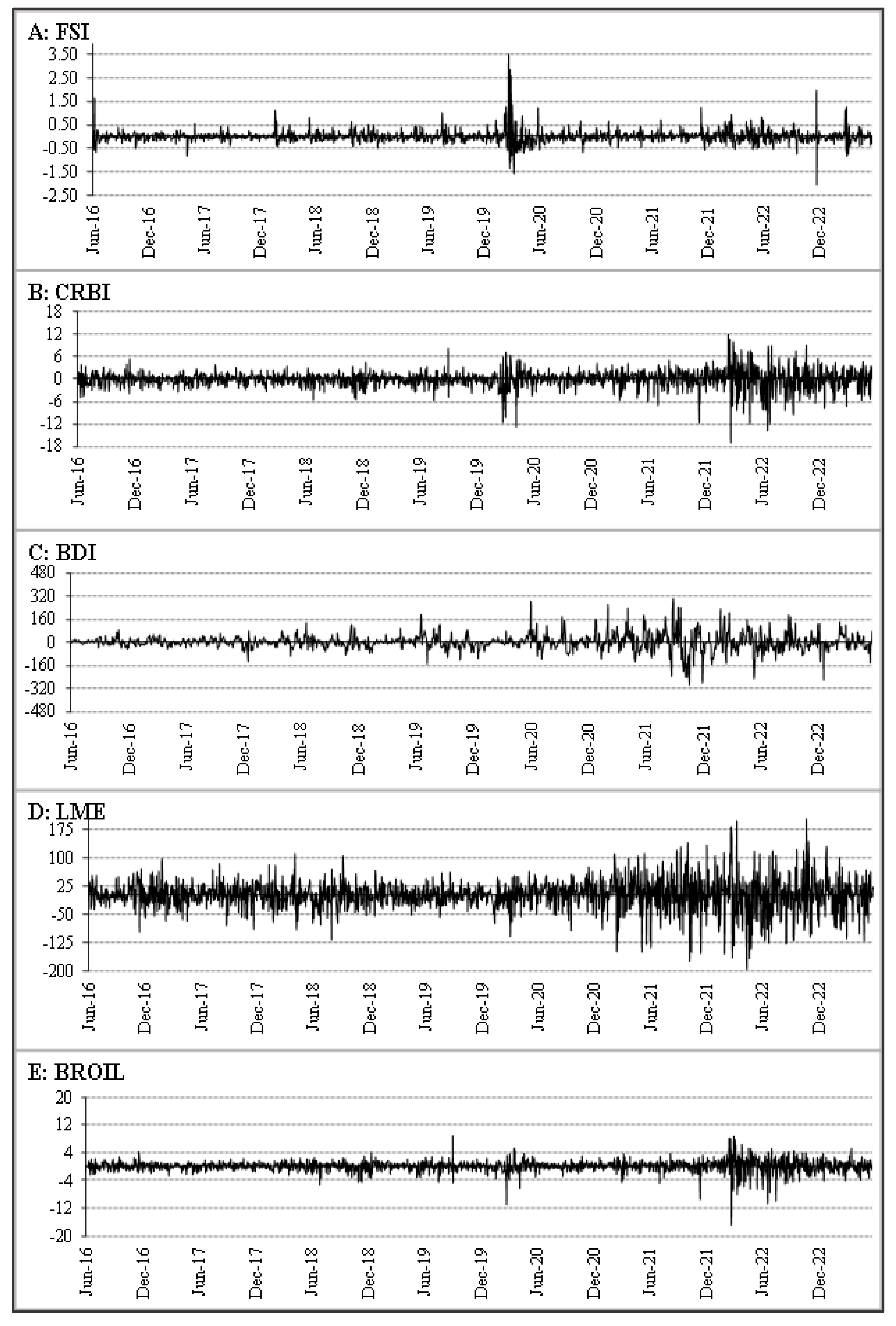
Figure 2. plots the daily change of the FSI and the commodity indices selected for this study. Daily change pathways show volatility clusters and high volatility. The FSI index daily change shows variation spikes in different time periods. When we plotted temporal changes of the FSI, stress spikes were observed during global stress events in the sample period, i.e., US-China trade tension, Covid-19 pandemic, and the Russian invasion of Ukraine. The highest stress spike was during the Covid-19 pandemic from late 2020 to mid-2021 which is the steepest in the whole sample period. The Ukraine Russia war is represented in the graph as the second stress full event, but this event lasts longer than the Covid-19 pandemic. FSI, CRBI and BROIL exhibited similar patterns and likeness in their volatile periods like trade tensions, Covid-19, and the Ukraine war. BDI and LME exhibited more volatile patterns than the others. From February 2018 to February 2020, a few factors may have contributed to the increased volatility of these indicators i.e., trade tensions during this period, as trade tension escalated between the US and China, as well as between other major trading partners. This uncertainty and disruption to global trade flows likely contributed to the BDI’s volatility. There were several instances of political instability during this period, including Brexit, protests in Hong Kong, and the ongoing conflict in the Middle East. These events may have contributed to the LME’s volatility, as investors reacted to the potential impacts of these events on global economic activity. The LME and BDI followed similar patterns in extreme events like COVID-19 from March 2020 and the Russia Ukraine war from Feb 2022 onwards.

3.2. Multifractal Detrended Cross Correlation Analysis (MFDCCA)

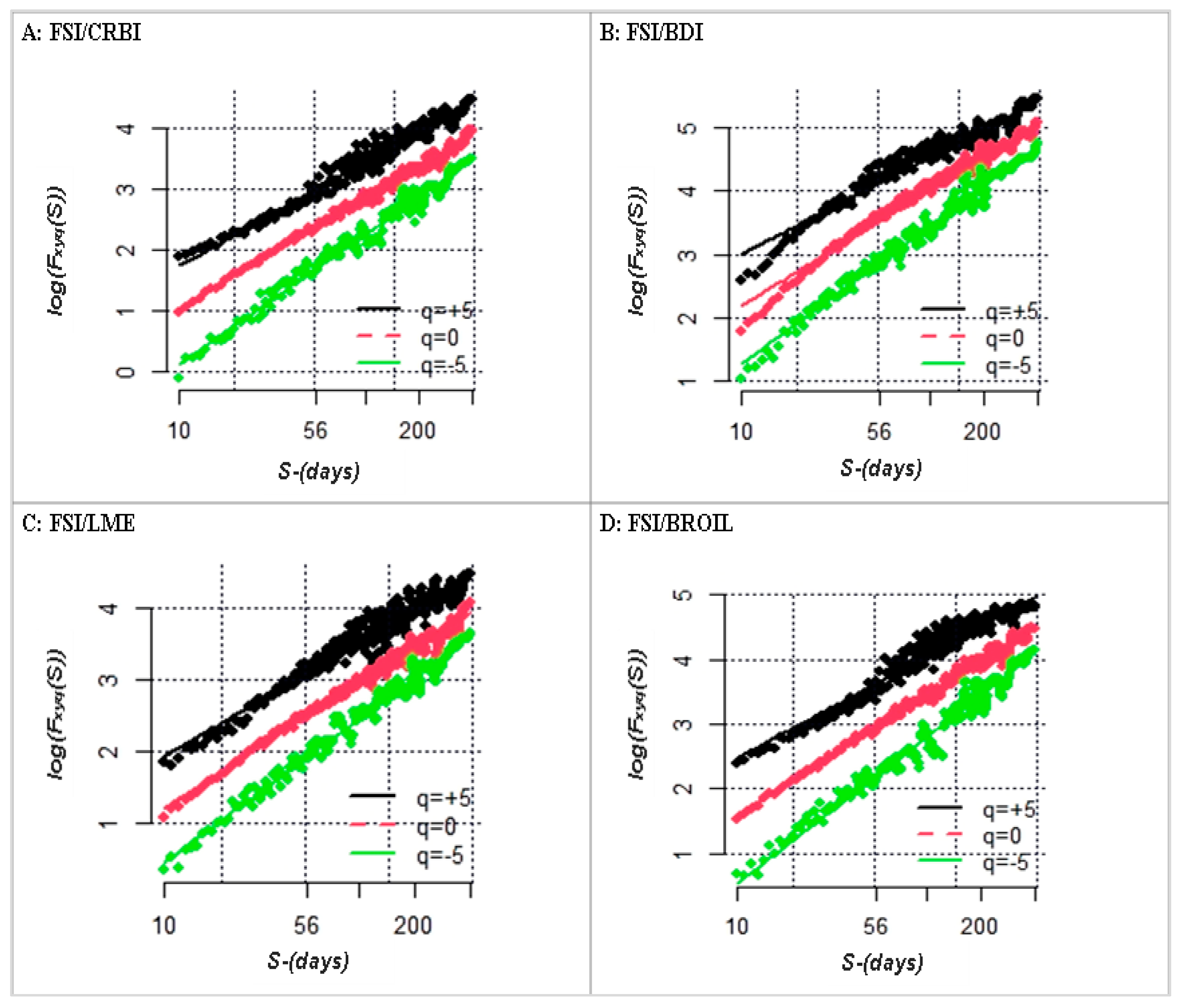
To compute the cross-correlation between FSI and commodity indices’ daily changes, we applied the existing multifractal detrended cross-correlation analysis. We determined the variability function Fxyq (S)) by increasing scaling order q from −5 to 5 step by step length, in line with the number of observations. Figure 3. plots the log - log movement of Fxyq (S)) depends on the time span s (days) between FSI and commodity indices’ daily changes of CRBI (Panel-A), BDI (Panel-B), LME (Panel-C) and BROIL(Panel-D). The lines rising from lowest to the highest relate to subsequent scale orders F x y q S for q = -5, q = 0, and q = +5. It is clear that F ( x y q S ) is well-shaped and exhibits an increasing trend with the gradual linear rise with the scale s orders, showing there is a power law correlation between FSI and four time series of commodity indices.
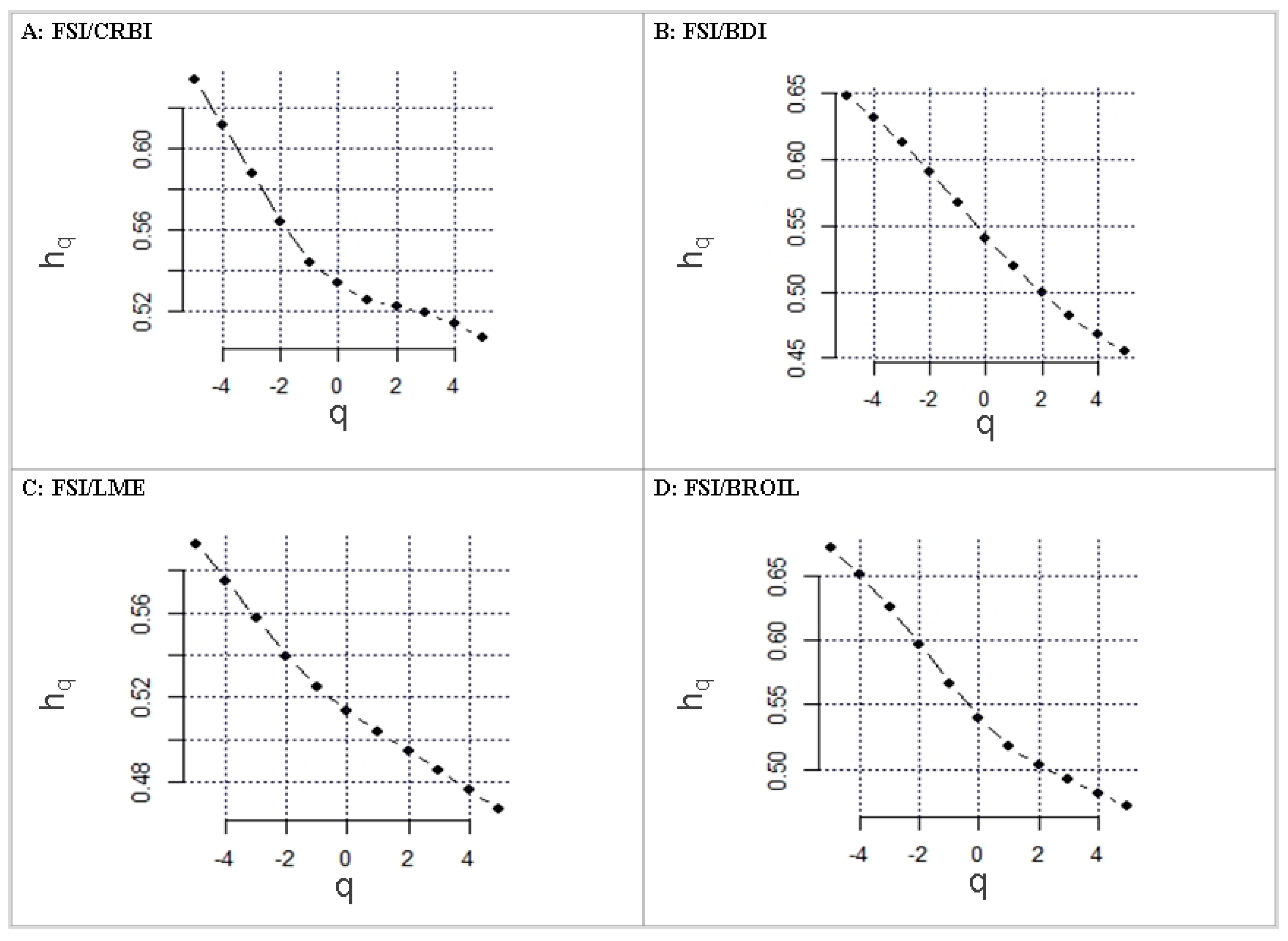
The result of the Hurst exponent between FSI and commodity market returns shows a declining trend as the order of q increases. As the highest value of Hxy(q) for FSI-BROIL reported in (column 5) Table 3, is 0.672 when q=-5, decreases to 0.540 at q=0 and further declines to 0.472 when q=5. A similar pattern is observed in the FSI-BDI pair Hurst index i.e., 0.648, 0.581 and 0.455 at q=-5, q=0 and q=5 respectively. The same pattern is followed by the FSI-CRBI pair, the highest Hurst index 0.633 when hq=-5, while 0.543 and .507 when hq=0 and hq=5 respectively. The lowest Hurst index score is found in the FSI-LME pair, which is 0.612 with the order of q=-5, declining to 0.545 with the order of q=0 and reaching 0.496 with the order of q=5. The declining structure is found in the Hurst exponents of all FSI and commodity market index pairs. The declining trend is evidence of multifractality in the time variations in the pairs of FSI and commodity market indices’ daily change. The results show that the Hurst exponent scores between FSI and selected commodities’ return series behave with a declining trend, as long as the time scale rises. Further, they show that H x y q values for q < 0 are all greater than the values of q > 0 , confirmation of the more persistent cross correlation pattern for minor variations than for large variations. Moreover, large variations have week cross-correlation compared to small variations, because H x y q for smaller and large variations declines as the order of scaling q rises.
The Table 3 further reports the findings of H x y ( q = 2 ) , which quantify the level of persistence among the cross correlations of the FSI and commodity market indices’ returns. Interestingly, the Hxy(q=2) score for FSI and the commodities CRBI and BROIL is greater than 0.5, which is evidence of the persistent behavior between the FSI and the selected commodity market indices’ daily price change.
Three different interpretations of these data are offered by the literature. A cross-persistent series is represented by Hxy(2)>0.5, and a positive (negative) value of Δ x t y t , denotes a significant probability of another positive (negative) value of Δ x t + 1 y t + 1 as claimed by [92]. [86] and [93] assert that long-term cross correlation implies that each series has a long memory of both its own past values and the past values of the other series. According to [94], power-law cross-correlations show that a change in one series will be followed by a change in the other. Considering these ideas, we can claim that a rise (fall) in the FSI is likely to be followed by a decrease (increase) in commodity market prices’ daily change.
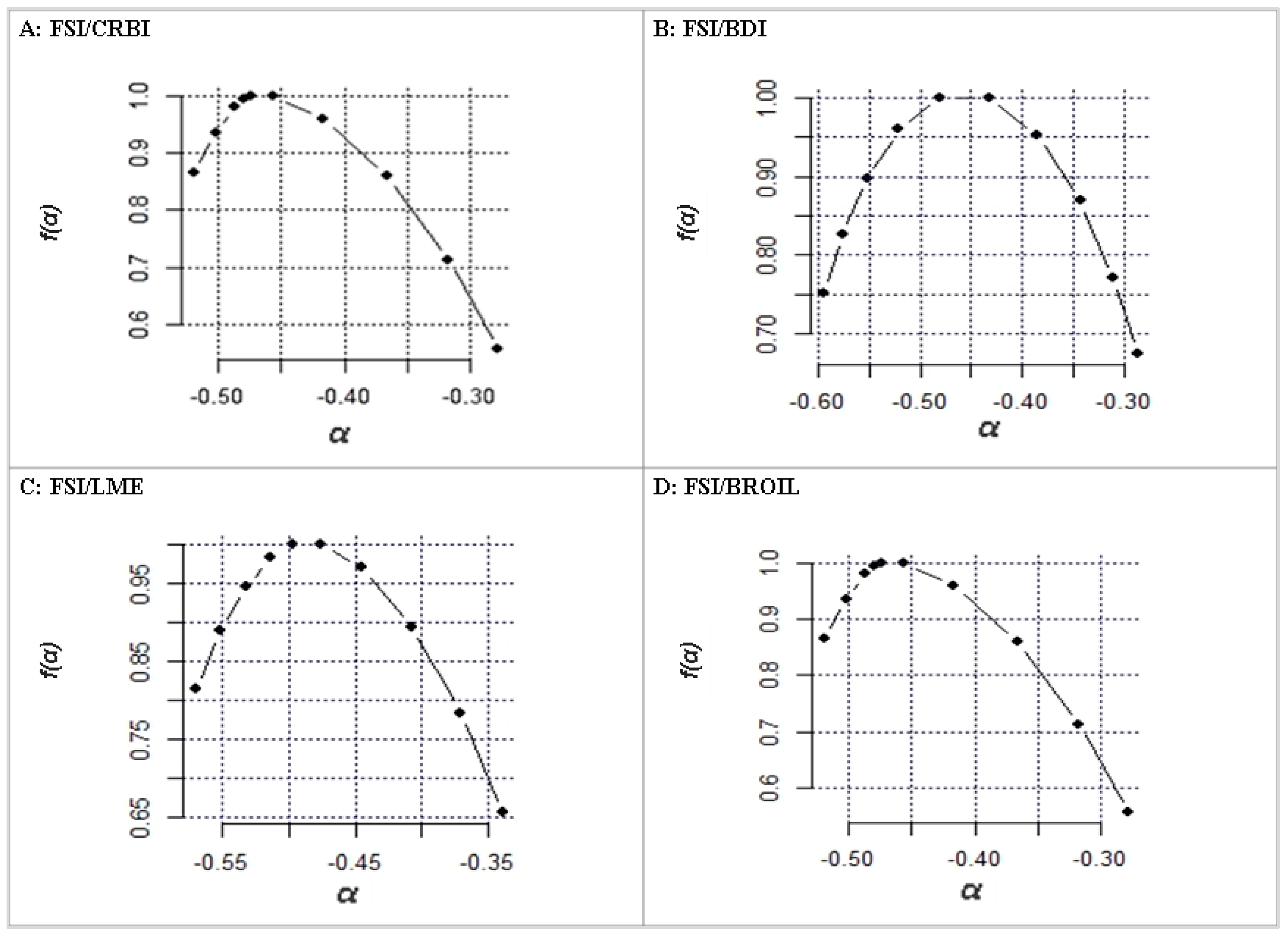
Table 4 reports the summary of the multifractal indices. The Hurst-exponent-average values lie between 0.5 and 0.6, indicating intensity or level of multifractality. However, the values of H are significantly higher than zero, establishing that the cross-correlations between FSI and commodity indices show robust multifractal patterns. A few interesting insights emerge, for instance, a degree of multifractal persistence that varies, with the maximum multifractality in the FSI-BROIL pair (∆H=0.2001) followed by FSI-BDI (∆H=0.193) then FSI-CRBI (∆H=0.126), while FSI-LME (∆H=0.125) has the lowest multifractality of the pairs under study. This shows that BROIL and BDI have the highest multifractality cross-correlation, while the LME and CRBI show a similarly low level of multifractality in the cross-correlations with FSI. These results can be confirmed by Figure 3, Figure 4 and Figure 5, as well as by the results of ∆α in column 4 of Table 4. Figure 5 represents the association between log(s) and log (F_xyq (S)) for q=-5 (green), q=0 (red) and q=5 (black), stretched with time length s for all the pairs of FSI with commodity market indices CRBI, BDI, LME and BROIL. The log-log plots are mapped well and increasing linearly as the scale s increases, meaning that power-law behavior and long-range cross-correlations occur between the FSI and commodity markets. The power-law cross-correlation infers that large variations in commodity market prices move to be complemented by the considerable variations in FSI and vice-versa. The higher width here is evidence of more variations, indicating random and heterogeneous distribution, which points to the more unpredictable descriptions of the daily change in commodity market indices.
The significant difference from zero spans of the cross-correlations’ multifractal progressions corroborates the obvious deviations from the random walk process. The AMH’s assumptions are backed up by evidence in favor of multifractality in the cross-correlation form [95], which has also been demonstrated in earlier research [96,97,98].
vs. α.
The degree of asymmetry results is reflected in column 5 of Table 4. The FSI-CRBI pair represented the highest AI value (3.968) followed by the FSI-BROIL pair (2.204) and FSI-BDI showed the lowest asymmetry AI value (1.285). Interestingly all commodity market indices paired with FSI show right skewed cross-correlations. When the value of the A I > 1 cross-correlation between the pair is right skewed contrary to the A I < 1 , is left skewed cross correlations. Additionally, outcomes of the singularity ratio C, a truncation gauge, for almost all the pairs indicate more profound left side tails ( C > 1 ) of the spectrum f ( α ) , suggesting more potent singularities, and the cross-correlation has a multifractal synthesis that is impervious to small-scale local variations [99].
The findings of singularity ratio C are reported on the right side of the last column of Table 4, where FSI-BDI is (0.7607) followed by FSI-LME (0.541) then FSI-BROIL (0.469) and the least value of FSI-CRBI (0.302). Interestingly, similar to the findings of ( A I ) , all commodity market indices showed ( C > 1 ) , indicating strong singularities and the cross-correlations have a multifractal formation that reacts promptly to local fluctuations even with small variations [99].
Past literature shows that long-range cross-correlations, fat-tails and intermittency are the main features of multifractality in the commodity markets. Cross-correlation indicates that the indices’ oscillations over longer time scales rely heavily on their past behavior rather than being independent of one another. The persistence or anti-persistence trends, loops, or volatility in the indices can lead to long-range correlations. The Hurst exponent, which runs between 0 and 1, can be used to calculate long-range correlations. An approximate Hurst exponent of 0.5 signals an arbitrary process, while an approximate Hurst exponent of 0 or 1 indicates either high persistence or anti-persistence, respectively. Fat-tails indicate the probable occurrence of extreme events (such as sharp price movements or crashes) is higher than would be estimated from a normal distribution in cases of fat-tailed distributions. The assortment of market participants, complicated feedback actions, the existence of outliers or aberrations in the data, or all these factors, can lead to fat-tailed distributions. Kurtosis, a measurement of how peaked or flat a distribution is in comparison to a normal distribution, can be used to identify fat-tailed distributions. A normal distribution is indicated by a kurtosis that is near to 3, whereas a fat-tailed distribution is indicated by a kurtosis that is higher than 3. Intermittency describes how the indices’ variations fluctuate in intensity throughout a range of time scales rather than being uniform. The multiscale structure of market activity, including the various trading frequencies, methods, and horizons of market participants, can lead to intermittent activity. The scaling exponents, which express how the fluctuations alter with the observation time scale, can be used to quantify intermittentness. A multifractal process is indicated by a changing scaling exponent, whereas a self-similar process is shown by a constant scaling exponent.
In their study of the realized volatility series of the Shanghai Stock Exchange Composite Index (SSEC) and the Shenzhen Stock Exchange Composite Index (SZSEC), [100] discovered that both indices displayed multifractality. Additionally, they discovered that fat-tailed distributions had some effects on multifractality and that long-range correlations of minor and significant major variations were the primary drivers of multifractality. In order to look into the nonlinear dependency and multifractality in the price-volume associations of China’s and the US’s agricultural commodities’ futures markets, [101] used multifractal detrended cross-correlation analysis (MFDCCA). They reported that both markets’ price-volume interactions demonstrated multifractality, with the main contributors being long-range cross-correlations and fat-tailed distributions.
[102] explored the multifractal features of financial markets, including commodity markets, employing multifractal analysis techniques and multifractal models. They scrutinized the accumulating proof of multifractality in financial time series across many markets and time periods, and argued about its origins. Additionally, they highlighted how multifractal analysis might be used to assess market inefficiencies and improve risk management, along with other applications.

3.3. Rolling Windows Analysis

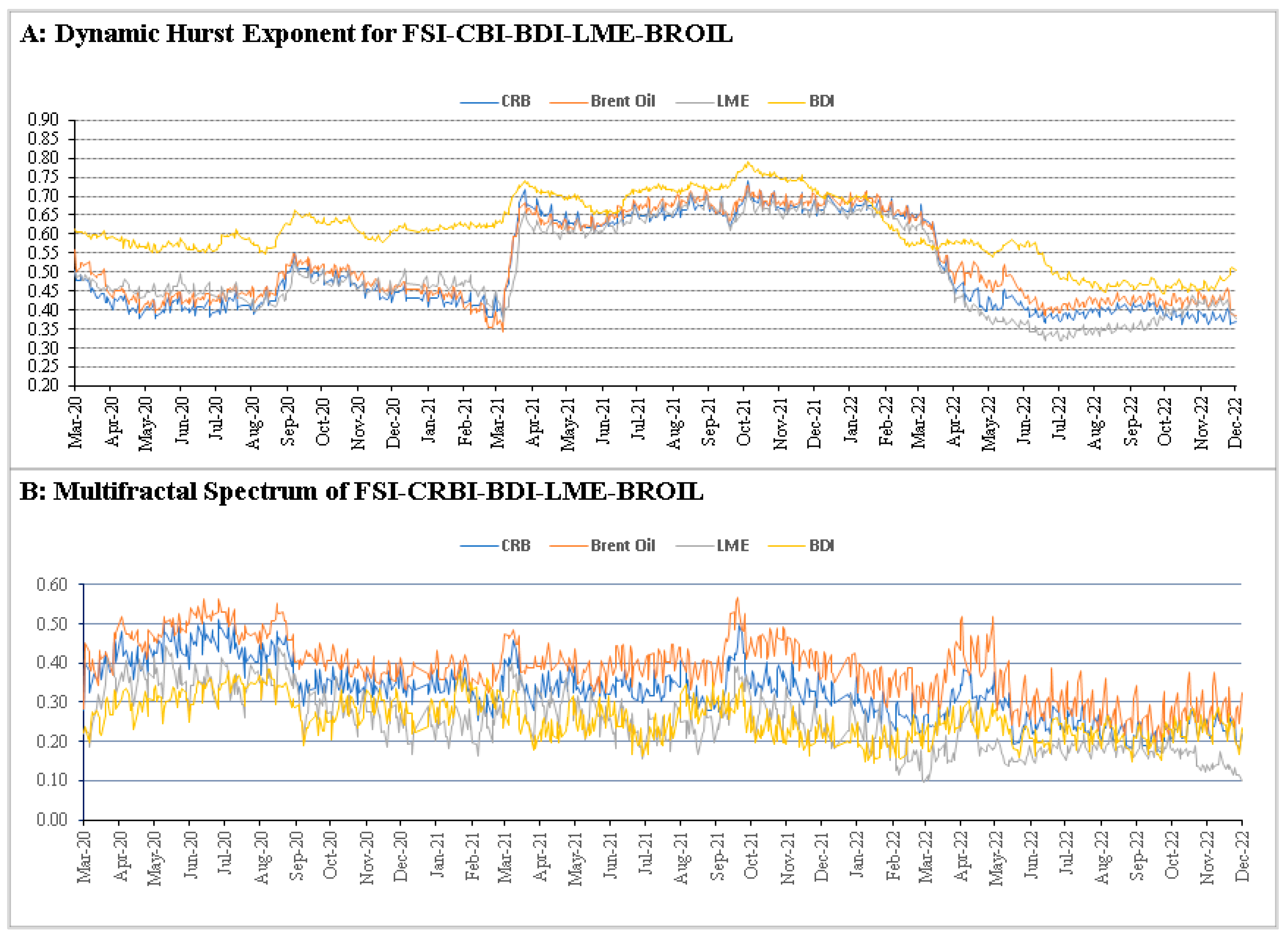
We use the MF-DCCA with rolling window technique to capture the dynamic changes in the cross-correlation between the FSI and the commodity market indices of CRBI, BDI, LME and BROIL. In Figure 6, Panel-A shows the evolution of the Hurst exponent (Q=2) across a rolling window of 500 trading days, whereas Panel-B shows the daily variations in multifractal strength. It is easily seen that the BDI exponent line remained above the other three commodity pairs and above 0.5 until July 2022, demonstrating a reliable cross-correlation persistence between the daily changes of BDI and FSI. The other three commodities, CRBI, BROIL, and LME, exhibit anti-persistence with the FSI before March 2021, persistent cross-correlation through the middle of 2022, and then a return to anti-persistence. The BROIL has the highest multifractality based on DH value, whereas LME demonstrates the lowest multifractal cross-correlation with the FSI, which is consistent with the overall results. In general, all commodity returns in 2020 exhibit significant multifractality in contrast to slightly lower DH values in the months following March 2022.

4. Conclusion

The purpose of this study is to measure the multifractal cross-correlations between the FSI and four commodity market indices, which represent the prices of numerous commodities: the CRBI, BDI, LME, and BROIL. We used the daily data from June 16, 2016, to June 9, 2023. We used Zhou’s (2008) multifractal detrended cross-correlation analysis (MFDCCA) to investigate the dynamic relationships between the returns of the commodity market indices and the financial stability index (FSI). This approach is helpful in revealing the long-term memory, tenacity, and mysterious behavior of the cross-correlations between financial stress and commodity returns, as well as their complex geometry and multifractality. To summarize, our findings corroborate the existence of cross-correlation by showing a connection between daily fluctuations in the FSI and commodity market indices. The power-law cross-correlation relationship shows that large price fluctuations in the commodity markets are more likely to follow notable changes in the FSI. Additionally, different levels of multifractality are seen; the FSI and BROIL show higher levels of multifractality, whilst the FSI and LME have the lowest multifractal cross-correlation. Furthermore, the consistent persistent cross-correlation behavior between the FSI and all chosen commodity market indices is confirmed by the Generalized Hurst Exponent (q=2) results. These results imply that financial and commodity indices retain a long-term memory of their respective historical lag values in addition to the historical values of the associated variable [92]. One could contend that changes in the FSI are also reflected in changes in returns on commodity markets [94]. Furthermore, the data demonstrate that all of the H x y q values for q<0 are greater than the values for q>0, suggesting that minor fluctuations exhibit a more persistent cross-correlation characteristic than do large fluctuations. All commodity-FSI pairs with FSI show a longer right tail (C<1) and a multifractal structure in their cross-correlations that is insensitive to local fluctuations with large magnitudes, according to the findings of the singularity ratio C. Conversely, none of the commodity-FSI pairs shows deeper left side tails (C >1) of the spectrum f(α), indicating stronger singularities and a multifractal structure in their cross-correlations that are not sensitive to local fluctuations with small magnitudes [99].
These results, notwithstanding certain restrictions, have a number of theoretical and applied consequences. Standard linear specifications, for instance, are not appropriate for modeling the cross-correlations among commodity markets, especially when it comes to the FSI. According to multiple econophysics research [53,93], the relationships between economic variables are inherently nonlinear. This finding is consistent with those studies. The cross-correlations’ nonlinear dependence indicates that any changes in FSI will have an effect on the return and volatility of the indexes tracking commodity markets. Accordingly, by modifying the commodity holdings in accordance with changes in FSI, portfolio management strategies using FSI can be put into practice [103]. Moreover, the quantification of small and big fluctuations by the MFDCCA model reveals an imbalance in the fractal complexity between the oscillations of the commodity market with varying amplitudes and the FSI. Key commodity markets’ cross-correlation provides insight into the regulation and control of the macroeconomy. As a result, in order to prevent any significant swings in the commodity markets, regulators of these markets must continuously develop regulations that take into account the broader impact on them. Furthermore, we recommend that market players separate the market connections between commodity indices and FSI in order to better formulate policies. As a result, our research offers a framework for investigating the relationships between financial stress and commodity market returns, as well as a basis for investigating similar content in other global markets.

Author Contributions

Conceptualization, H.A and F.A.; Data curation, F.A and P.F.; Formal analysis, F.A and H.A; Writing—original draft, H.A and F.A; Writing—review & editing, P.F and H.A.

Data Availability Statement

The data sets used in this study are openly available.

Conflicts of Interest

The authors declare no conflict of interest.

References

  1. Moore, R.; Mao, Y.; Zhang, J.; Clarke, K. Economic burden of illness in Canada, 1993. Chronic Diseases and Injuries in Canada 1997, 18, 1F. [Google Scholar]
  2. Jahoda, M. Economic recession and mental health: Some conceptual issues. Journal of social Issues 1988, 44, 13–23. [Google Scholar] [CrossRef]
  3. Huang, R.; Ghose, B.; Tang, S. Effect of financial stress on self-reported health and quality of life among older adults in five developing countries: a cross sectional analysis of WHO-SAGE survey. BMC geriatrics 2020, 20, 1–12. [Google Scholar] [CrossRef]
  4. Sturgeon, J.A.; Arewasikporn, A.; Okun, M.A.; Davis, M.C.; Ong, A.D.; Zautra, A.J. The psychosocial context of financial stress: Implications for inflammation and psychological health. Psychosomatic medicine 2016, 78, 134. [Google Scholar] [CrossRef] [PubMed]
  5. Taylor, M.; Stevens, G.; Agho, K.; Raphael, B. The impacts of household financial stress, resilience, social support, and other adversities on the psychological distress of Western Sydney parents. International Journal of Population Research 2017, 2017. [Google Scholar] [CrossRef]
  6. Åslund, C.; Larm, P.; Starrin, B.; Nilsson, K.W. The buffering effect of tangible social support on financial stress: influence on psychological well-being and psychosomatic symptoms in a large sample of the adult general population. International journal for equity in health 2014, 13, 1–9. [Google Scholar] [CrossRef]
  7. Altman, E.I.; Hotchkiss, E. Corporate financial distress and bankruptcy. John Wiley & Sons: New York, 1993; Volume 1998. [Google Scholar]
  8. Davis, C.G.; Mantler, J. The consequences of financial stress for individuals, families, and society. Centre for Research on Stress, Coping and Well-being. Carleton University, Ottawa, 2024. [Google Scholar]
  9. Frank, C.; Davis, C.G.; Elgar, F.J. Financial strain, social capital, and perceived health during economic recession: a longitudinal survey in rural Canada. Anxiety, Stress, & Coping 2014, 27, 422–438. [Google Scholar]
  10. Koh, S.; Durand, R.B.; Dai, L.; Chang, M. Financial distress: Lifecycle and corporate restructuring. Journal of Corporate Finance 2015, 33, 19–33. [Google Scholar] [CrossRef]
  11. Setiany, E. The effect of investment, free cash flow, earnings management, and interest coverage ratio on financial distress. Journal of Social Science 2021, 2, 64–69. [Google Scholar]
  12. Efthyvoulou, G. The impact of financial stress on sectoral productivity. Economics Letters 2012, 116, 240–243. [Google Scholar] [CrossRef]
  13. Karolyi, G.A. The consequences of terrorism for financial markets: what do we know? Available at SSRN 904398 2006. [Google Scholar] [CrossRef]
  14. Cardarelli, R.; Elekdag, S.A.; Lall, S. Financial stress, downturns, and recoveries. 2009.
  15. Ahir, H.; Dell’Ariccia, G.; Furceri, D.; Papageorgiou, C.; Qi, H. Financial Stress and Economic Activity. IMF Research Department 2023. [Google Scholar]
  16. Mundra, S.; Bicchal, M. Asymmetric effects of monetary policy and financial accelerator: Evidence from India. The Journal of Economic Asymmetries 2023, 27, e00296. [Google Scholar] [CrossRef]
  17. Apostolakis, G.; Papadopoulos, A.P. Financial stress spillovers in advanced economies. Journal of International Financial Markets, Institutions and Money 2014, 32, 128–149. [Google Scholar] [CrossRef]
  18. Ishrakieh, L.M.; Dagher, L.; El Hariri, S. A financial stress index for a highly dollarized developing country: The case of Lebanon. Central Bank Review 2020, 20, 43–52. [Google Scholar] [CrossRef]
  19. Ilesanmi, K.D.; Tewari, D.D. Financial stress index and economic activity in South Africa: New evidence. Economies 2020, 8, 110. [Google Scholar] [CrossRef]
  20. Cevik, E.I.; Dibooglu, S.; Kenc, T. Financial stress and economic activity in some emerging Asian economies. Research in International Business and Finance 2016, 36, 127–139. [Google Scholar] [CrossRef]
  21. Hubrich, K.; Tetlow, R.J. Financial stress and economic dynamics: The transmission of crises. Journal of Monetary Economics 2015, 70, 100–115. [Google Scholar] [CrossRef]
  22. Apostolakis, G.; Papadopoulos, A.P. Financial stability, monetary stability and growth: a PVAR analysis. Open Economies Review 2019, 30, 157–178. [Google Scholar] [CrossRef]
  23. Ozcelebi, O. Assessing the impacts of financial stress index of developed countries on the exchange market pressure index of emerging countries. International Review of Economics & Finance 2020, 70, 288–302. [Google Scholar]
  24. Vermeulen, R.; Hoeberichts, M.; Vašíček, B.; Žigraiová, D.; Šmídková, K.; de Haan, J. Financial stress indices and financial crises. Open Economies Review 2015, 26, 383–406. [Google Scholar] [CrossRef]
  25. Altman, E.I.; Hotchkiss, E. Corporate financial distress and bankruptcy: Predict and avoid bankruptcy, analyze and invest in distressed debt; John Wiley & Sons: 2010; Volume 289.
  26. Jadoon, I.A.; Mumtaz, R.; Sheikh, J.; Ayub, U.; Tahir, M. The impact of green growth on financial stability. Journal of Financial Regulation and Compliance 2021, 29, 533–560. [Google Scholar] [CrossRef]
  27. Geetha, K.; Suganthi, L.M.; Vasanthi, K.; Kavitha, B. Financial stress testing in US banking sector. Materials Today: Proceedings 2021, 37, 2252–2255. [Google Scholar] [CrossRef]
  28. Cardarelli, R.; Elekdag, S.; Lall, S. Financial stress and economic contractions. Journal of Financial Stability 2011, 7, 78–97. [Google Scholar] [CrossRef]
  29. Cevik, E.I.; Dibooglu, S.; Kutan, A.M. Measuring financial stress in transition economies. Journal of financial stability 2013, 9, 597–611. [Google Scholar] [CrossRef]
  30. Chen, L.; Verousis, T.; Wang, K.; Zhou, Z. Financial stress and commodity price volatility. Energy Economics 2023, 125, 106874. [Google Scholar] [CrossRef]
  31. Xu, Y.; Liang, C.; Wang, J. Financial stress and returns predictability: Fresh evidence from China. Pacific-Basin Finance Journal 2023, 78, 101980. [Google Scholar] [CrossRef]
  32. Hoque, M.E.; Soo-Wah, L.; Tiwari, A.K.; Akhter, T. Time and frequency domain connectedness and spillover among categorical and regional financial stress, gold and bitcoin market. Resources Policy 2023, 85, 103786. [Google Scholar] [CrossRef]
  33. Mezghani, T.; Boujelbène, M.; Boutouria, S. Forecasting the impact of financial stress on hedging between the oil market and GCC financial markets. Managerial Finance 2023. [Google Scholar] [CrossRef]
  34. Sohag, K.; Kalina, I.; Elsayed, A.H. Financial stress in Russia: Exploring the impact of oil market shocks. Resources Policy 2023, 86, 104150. [Google Scholar] [CrossRef]
  35. Adam, T.; Benecká, S.; Matějů, J. Financial stress and its non-linear impact on CEE exchange rates. Journal of Financial Stability 2018, 36, 346–360. [Google Scholar] [CrossRef]
  36. Apostolakis, G.; Papadopoulos, A.P. Financial stress spillovers across the banking, securities and foreign exchange markets. Journal of Financial Stability 2015, 19, 1–21. [Google Scholar] [CrossRef]
  37. Li, Y.; Liang, C.; Huynh, T.L.D. Combination forecast based on financial stress categories for global equity market volatility: the evidence during the COVID-19 and the global financial crisis periods. Applied Economics 2023, 1–36. [Google Scholar] [CrossRef]
  38. Armah, M.; Bossman, A.; Amewu, G. Information flow between global financial market stress and African equity markets: An EEMD-based transfer entropy analysis. Heliyon 2023, 9. [Google Scholar] [CrossRef] [PubMed]
  39. Bossman, A.; Armah, M.; Amewu, G. Information Flow between Global Financial Market Stress and African Equity Markets: An Eemd-Based Transfer Entropy Analysis. In Information Flow between Global Financial Market Stress and African Equity Markets: An Eemd-Based Transfer Entropy Analysis: Bossman, Ahmed| uArmah, Mohammed| uAmewu, Godfred; [Sl]: SSRN: 2022.
  40. Chau, F.; Deesomsak, R. Does linkage fuel the fire? The transmission of financial stress across the markets. International Review of Financial Analysis 2014, 36, 57–70. [Google Scholar] [CrossRef]
  41. Sousa, R.M. Wealth-to-income ratio, government bond yields and financial stress in the Euro Area. Applied Economics Letters 2012, 19, 1085–1088. [Google Scholar] [CrossRef]
  42. Liang, C.; Hong, Y.; Huynh, L.D.T.; Ma, F. Asymmetric dynamic risk transmission between financial stress and monetary policy uncertainty: thinking in the post-covid-19 world. Review of Quantitative Finance and Accounting 2023, 60, 1543–1567. [Google Scholar] [CrossRef]
  43. Gomis-Porqueras, P.; Ruprecht, R. A Financial Stress Index for a Small Open Economy: The Australian Case. 2023.
  44. Zhang, H.; Wang, P. Does Bitcoin or gold react to financial stress alike? Evidence from the US and China. International Review of Economics & Finance 2021, 71, 629–648. [Google Scholar]
  45. Reboredo, J.C.; Uddin, G.S. Do financial stress and policy uncertainty have an impact on the energy and metals markets? A quantile regression approach. International Review of Economics & Finance 2016, 43, 284–298. [Google Scholar]
  46. Miah, M.D.; Shafiullah, M.; Alam, M.S. The effect of financial stress on renewable energy consumption: evidence from US data. Environment, Development and Sustainability 2023, 1–24. [Google Scholar] [CrossRef]
  47. Apostolakis, G.N.; Floros, C.; Gkillas, K.; Wohar, M. Financial stress, economic policy uncertainty, and oil price uncertainty. Energy Economics 2021, 104, 105686. [Google Scholar] [CrossRef]
  48. Xiang, J.; Chen, H.; Li, L. Oil Price Uncertainty, Financial Distress and Real Economic Activities: Evidence from China. Financial Distress and Real Economic Activities: Evidence from China.
  49. Cifarelli, G.; Paladino, G. A dynamic model of hedging and speculation in the commodity futures markets. Journal of Financial Markets 2015, 25, 1–15. [Google Scholar] [CrossRef]
  50. Chen, Y.-F.; Mu, X. Asymmetric volatility in commodity markets. Journal of Commodity Markets 2021, 22, 100139. [Google Scholar] [CrossRef]
  51. Ghoshray, A. Do international primary commodity prices exhibit asymmetric adjustment? Journal of Commodity Markets 2019, 14, 40–50. [Google Scholar] [CrossRef]
  52. Andreasson, P.; Bekiros, S.; Nguyen, D.K.; Uddin, G.S. Impact of speculation and economic uncertainty on commodity markets. International review of financial analysis 2016, 43, 115–127. [Google Scholar] [CrossRef]
  53. Liu, L. Cross-correlations between crude oil and agricultural commodity markets. Physica A: Statistical Mechanics and its Applications 2014, 395, 293–302. [Google Scholar] [CrossRef]
  54. Bhardwaj, G.; Janardanan, R.; Rouwenhorst, K.G. The first commodity futures index of 1933. Journal of Commodity Markets 2021, 23, 100157. [Google Scholar] [CrossRef]
  55. Aepli, M.D.; Füss, R.; Henriksen, T.E.S.; Paraschiv, F. Modeling the multivariate dynamic dependence structure of commodity futures portfolios. Journal of commodity Markets 2017, 6, 66–87. [Google Scholar] [CrossRef]
  56. Mulvey, J.M.; Kim, W.C.; Lin, C. Optimizing a portfolio of liquid and illiquid assets. Optimal Financial Decision Making under Uncertainty 2017, 151–175. [Google Scholar]
  57. Monin, P.J. The OFR financial stress index. Risks 2019, 7, 25. [Google Scholar] [CrossRef]
  58. Robillard, R.; Saad, M.; Edwards, J.; Solomonova, E.; Pennestri, M.-H.; Daros, A.; Veissière, S.P.L.; Quilty, L.; Dion, K.; Nixon, A. Social, financial and psychological stress during an emerging pandemic: observations from a population survey in the acute phase of COVID-19. BMJ open 2020, 10, e043805. [Google Scholar] [CrossRef] [PubMed]
  59. Wan, Y.; Wang, W.; He, S.; Hu, B. How do uncertainties affect the connectedness of global financial markets? Changes during the Russia-Ukraine conflict. Asia-Pacific Journal of Accounting & Economics, 2024; 1–28. [Google Scholar]
  60. Li, Z.-C.; Xie, C.; Zeng, Z.-J.; Wang, G.-J.; Zhang, T. Forecasting global stock market volatilities in an uncertain world. International Review of Financial Analysis 2023, 85, 102463. [Google Scholar] [CrossRef]
  61. Adrian, T. Safeguarding Financial Stability amid High Inflation and Geopolitical Risks. Available online: https://www.imf.org/en/Blogs/Articles/2023/04/11/global-financial-system-tested-by-higher-inflation-and-interest-rates (accessed on .
  62. Shahzad, U.; Mohammed, K.S.; Tiwari, S.; Nakonieczny, J.; Nesterowicz, R. Connectedness between geopolitical risk, financial instability indices and precious metals markets: Novel findings from Russia Ukraine conflict perspective. Resources Policy 2023, 80, 103190. [Google Scholar] [CrossRef]
  63. Ahmed, F. Unravelling the Spillover Effects of Uncertainty and Russian Financial Stress Index During Russia-Ukraine Conflict. Available at SSRN 459 7224.
  64. Gadanecz, B.; Jayaram, K. Measures of financial stability-a review. Irving Fisher Committee Bulletin 2008, 31, 365–383. [Google Scholar]
  65. Consolini, G.; De Michelis, P. A Joint Multifractal Approach to Solar Wind Turbulence. Fractal and Fractional 2023, 7, 748. [Google Scholar] [CrossRef]
  66. Zhou, W.-X. Multifractal detrended cross-correlation analysis for two nonstationary signals. Physical Review E 2008, 77, 066211. [Google Scholar] [CrossRef] [PubMed]
  67. Kojić, M.; Mitić, P.; Minović, J. Gold and Sustainable Stocks in the US and EU: Nonlinear Analysis Based on Multifractal Detrended Cross-Correlation Analysis and Granger Causality. Fractal and fractional 2023, 7, 738. [Google Scholar] [CrossRef]
  68. Duanzhu, S.; Wang, J.; Jia, C. Hotel Comment Emotion Classification Based on the MF-DFA and Partial Differential Equation Classifier. Fractal and Fractional 2023, 7, 744. [Google Scholar] [CrossRef]
  69. ECB. Financial Stability Review. Available online: https://www.ecb.europa.eu/pub/pdf/fsr/financialstabilityreview201206en.pdf (accessed on 11 October 2023).
  70. SARI, S.S. Predicting Financial Stress Index Using Wavelet Transform Artificial Neural Networks. The Journal of International Scientific Researches 2022, 7, 282–296. [Google Scholar] [CrossRef]
  71. Bhardwaj, G.; Gorton, G.; Rouwenhorst, G. Facts and fantasies about commodity futures ten years later; National Bureau of Economic Research: 2015.
  72. Acharya, R.N.; Gentle, P.F.; Paudel, K.P. Examining the CRB index as a leading indicator for US inflation. Applied Economics Letters 2010, 17, 1493–1496. [Google Scholar] [CrossRef]
  73. Acharya, R.N.; Gentle, P.F.; Mishra, A.K.; Paudel, K.P. Examining the CRB Index as an indicator for US inflation, 2008.
  74. Katris, C.; Kavussanos, M.G. Time series forecasting methods for the Baltic dry index. Journal of Forecasting 2021, 40, 1540–1565. [Google Scholar] [CrossRef]
  75. Bakshi, G.; Panayotov, G.; Skoulakis, G. The Baltic Dry Index as a predictor of global stock returns, commodity returns, and global economic activity. Commodity Returns, and Global Economic Activity (October 1, 2010) 2010.
  76. Bildirici, M.E.; Kayıkçı, F.; Onat, I.Ş. Baltic Dry Index as a major economic policy indicator: the relationship with economic growth. Procedia-Social and Behavioral Sciences 2015, 210, 416–424. [Google Scholar] [CrossRef]
  77. Han, L.; Wan, L.; Xu, Y. Can the Baltic Dry Index predict foreign exchange rates? Finance Research Letters 2020, 32, 101157. [Google Scholar] [CrossRef]
  78. Apergis, N.; Payne, J.E. New evidence on the information and predictive content of the Baltic Dry Index. International journal of financial studies 2013, 1, 62–80. [Google Scholar] [CrossRef]
  79. Watorek, M.; Drożdż, S.; Oświȩcimka, P.; Stanuszek, M. Multifractal cross-correlations between the world oil and other financial markets in 2012–2017. Energy Economics 2019, 81, 874–885. [Google Scholar] [CrossRef]
  80. Yarlagadda, H.; Patel, M.A.; Gupta, V.; Bansal, T.; Upadhyay, S.; Shaheen, N.; Jain, R.; Patel, M.; Bansal, T.K. COVID-19 vaccine challenges in developing and developed countries. Cureus 2022, 14. [Google Scholar] [CrossRef] [PubMed]
  81. Kasal, S. What are the effects of financial stress on economic activity and government debt? An empirical examination in an emerging economy. Borsa Istanbul Review 2023, 23, 254–267. [Google Scholar] [CrossRef]
  82. IMF. The outlook is uncertain again amid financial sector turmoil, high inflation, ongoing effects of Russia’s invasion of Ukraine, and three years of COVID. Available online: https://www.imf.org/en/Publications/WEO/Issues/2023/04/11/world-economic-outlook-april-2023 (accessed on 13 September 2023).
  83. EIA. TODAY IN ENERGY. Available online: https://www.eia.gov/todayinenergy/detail.php?id=34372 (accessed on 19 September 2023).
  84. de la Torre, J.C.; Pavón-Domínguez, P.; Dorronsoro, B.; Galindo, P.L.; Ruiz, P. Multi-Signal Multifractal Detrended Fluctuation Analysis for Uncertain Systems—Application to the Energy Consumption of Software Programs in Microcontrollers. Fractal and Fractional 2023, 7, 794. [Google Scholar] [CrossRef]
  85. Kristoufek, L. Multifractal height cross-correlation analysis: A new method for analyzing long-range cross-correlations. EPL (Europhysics Letters) 2011, 95, 68001. [Google Scholar] [CrossRef]
  86. Yuan, Y.; Zhuang, X.-t.; Jin, X. Measuring multifractality of stock price fluctuation using multifractal detrended fluctuation analysis. Physica A: Statistical Mechanics and its Applications 2009, 388, 2189–2197. [Google Scholar] [CrossRef]
  87. Telesca, L.; Thai, A.T.; Cao, D.T.; Cao, D.T.; Dinh, Q.V.; Mai, X.B. Fractal and Spectral Analysis of Seismicity in the Lai Chau Area (Vietnam). Fractal and Fractional 2023, 7, 776. [Google Scholar] [CrossRef]
  88. Freitas, D.B.d.; Nepomuceno, M.M.F.; Nepomuceno, M.M.F.; Leão, I.C.; Chagas, M.L.D.; Chagas, M.L.D.; Martins, B.L.C.; Medeiros, J.R.D. New Suns in the Cosmos. IV. The Multifractal Nature of Stellar Magnetic Activity in Kepler Cool Stars. The Astrophysical Journal 2017, 843. [Google Scholar] [CrossRef]
  89. Hampson, K.M.; Mallen, E.A. Multifractal nature of ocular aberration dynamics of the human eye. Biomedical optics express 2011, 2, 464–470. [Google Scholar] [CrossRef] [PubMed]
  90. Hurst, H.E. Long term storage. An experimental study 1965. [Google Scholar]
  91. Seuront, L. Fractals and multifractals in ecology and aquatic science; CRC Press: 2009.
  92. Kristoufek, L. Multifractal height cross-correlation analysis: A new method for analyzing long-range cross-correlations. Europhysics Letters 2011, 95, 68001. [Google Scholar] [CrossRef]
  93. Podobnik, B.; Wang, D.; Horvatic, D.; Grosse, I.; Stanley, H.E. Time-lag cross-correlations in collective phenomena. Europhysics Letters 2010, 90, 68001. [Google Scholar] [CrossRef]
  94. Podobnik, B.; Stanley, H.E. Detrended cross-correlation analysis: a new method for analyzing two nonstationary time series. Phys. Rev. Lett. 2008, 100, 084102. [Google Scholar] [CrossRef]
  95. Kristoufek, L.; Vosvrda, M. Measuring capital market efficiency: Global and local correlations structure. Physica A: Statistical Mechanics and its Applications 2013, 392, 184–193. [Google Scholar] [CrossRef]
  96. Hasan, R.; Salim, M.M. Power law cross-correlations between price change and volume change of Indian stocks. Physica A: Statistical Mechanics and its Applications 2017, 473, 620–631. [Google Scholar] [CrossRef]
  97. Ferreira, P. Assessing the relationship between dependence and volume in stock markets: A dynamic analysis. Physica A: Statistical Mechanics and its Applications 2019, 516, 90–97. [Google Scholar] [CrossRef]
  98. Ruan, Q.; Jiang, W.; Ma, G. Cross-correlations between price and volume in Chinese gold markets. Physica A: Statistical Mechanics and its Applications 2016, 451, 10–22. [Google Scholar] [CrossRef]
  99. Ihlen, E. Introduction to Multifractal Detrended Fluctuation Analysis in Matlab. Front. Physiol. 2012, 3. [Google Scholar] [CrossRef] [PubMed]
  100. Wang, G.-J.; Xiong, L.; Zhu, Y.; Xie, C.; Foglia, M. Multilayer network analysis of investor sentiment and stock returns. Research in International Business and Finance 2022, 62, 101707. [Google Scholar] [CrossRef]
  101. Cao, G.; Han, Y.; Cui, W.; Guo, Y. Multifractal detrended cross-correlations between the CSI 300 index futures and the spot markets based on high-frequency data. Physica A: Statistical Mechanics and its Applications 2014, 414, 308–320. [Google Scholar] [CrossRef]
  102. Jiang, Y.; Nie, H.; Ruan, W. Time-varying long-term memory in Bitcoin market. Finance Research Letters 2018, 25, 280–284. [Google Scholar] [CrossRef]
  103. Attig, N.; El Ghoul, S.; Guedhami, O.; Zheng, X. Dividends and economic policy uncertainty: International evidence. Journal of Corporate Finance 2021, 66, 101785. [Google Scholar] [CrossRef]
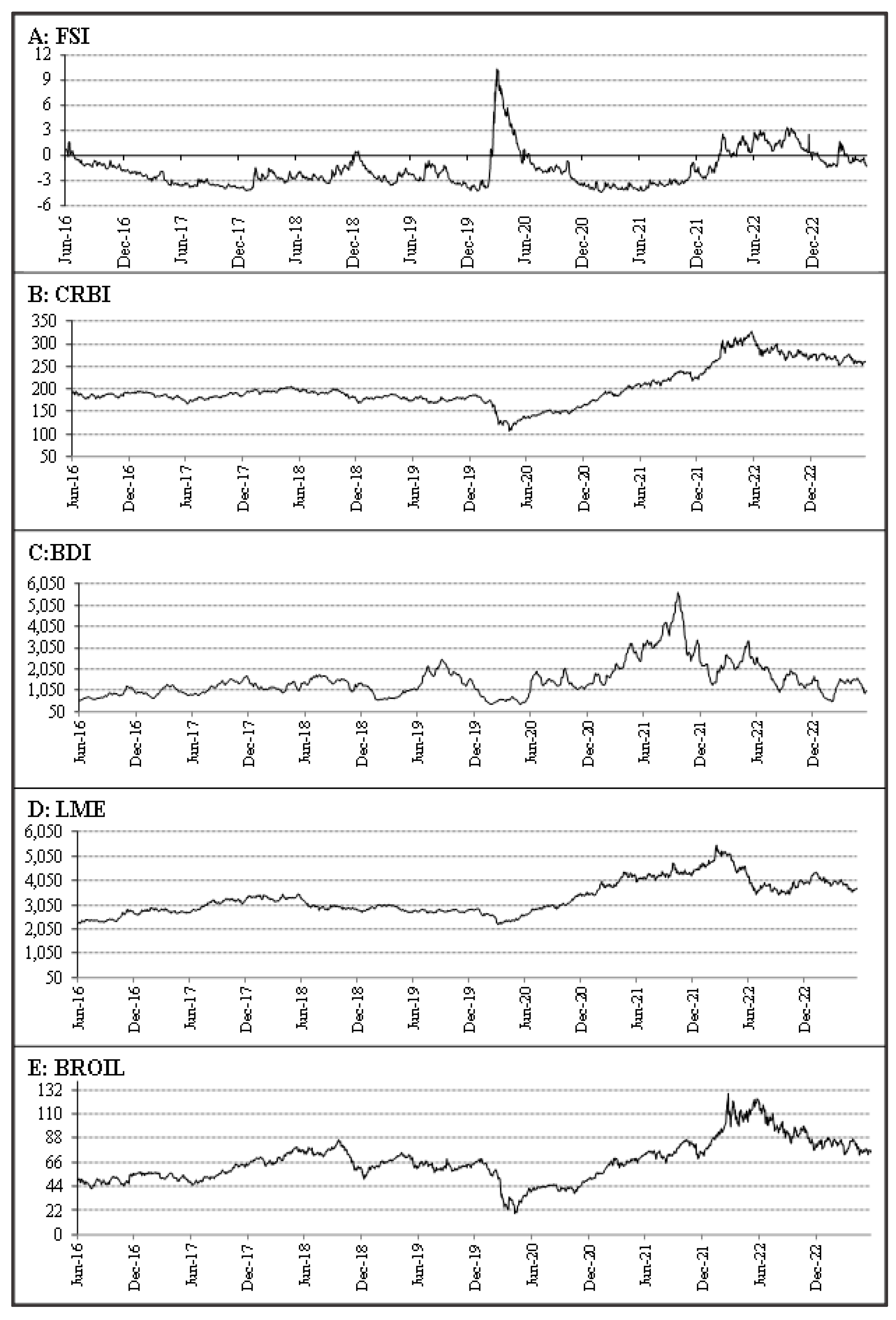
Figure 1. Daily Index values of FSI, CRBI, BDI, LME & BROIL.
Preprints 91077 g001
Figure 2. Daily Change of FSI, CRBI, BDI, LME & BROIL.
Preprints 91077 g002
Figure 3. Log-Log plot of Fluctuation functions Fxyq (S) versus s for q=[-5,0,+5].
Preprints 91077 g003
Figure 4. Generalized Hurst exponent Hxy dependence on q for q=-5, q=0, q=5.
Preprints 91077 g004
Figure 5. The Multiple Spectra of f ( α )
Preprints 91077 g005
Figure 6. Dynamic Hurst exponents evolution for FSI and Commodity Markets (q = 2 and window = 500).
Preprints 91077 g006
Table 1. Commodity Index Weights and Coverage.
Index Symbol Coverage Weights
Commodity Research Bureau Index CRBI Basket of 19 Agricultural, Energy and Food commodities 41% to agriculture, 39% to energy, and the remainder to others.
Baltic Dry Index BDI Shipping freight rates of coal, iron ore, and other commodities. 40% Capesize, 30% Supramax and Panamax 30% cost on shipping routes carrying coal, grains, iron ore, and other commodities.
London Metal Exchange LME Industrial Metals Aluminum, Copper, Zinc, Lead, Nickel and Tin. The average global production volume and trade liquidity for the previous five years are used to determine the weight of the six metals i.e., aluminum, copper, zinc, lead, nickel, and tin (42.8%, 31.2%, 14.8% 8.2%, 2% & 1%) respectively.
Brent Oil Price Index BROIL Brent Crude spot Prices per barrel in US dollars.
Table 2. Summary Statistics of FSI and Commodity Market Indices.
FSI CRBI BDI LME BROIL
Mean -0.0012 0.0386 0.2649 0.8367 0.0145
Standard Deviation 0.2695 2.3279 54.1240 40.3048 1.6843
Range 5.5010 28.82 594.0 400.0 25.64
Kurtosis 33.5989 6.0868 5.8149 2.9636 11.4127
Skewness 2.8494 -0.7096 0.1125 -0.1907 -1.1543
Jarque-Bera test 1022*** 1759*** 370*** 118*** 2305***
ADF -11.74*** -10.64*** -10.31*** 11.18*** -10.641***
Note: *** represents 99% significance level.
Table 3. Hurst exponent for FSI and Commodity Market ranging over qε(-5, 5).
Order FSI-CRBI FSI-BDI FSI-LME FSI-BROIL
-5 0.6335 0.6482 0.6124 0.6717
-4 0.6113 0.6319 0.5952 0.6506
-3 0.5873 0.6128 0.5879 0.6256
-2 0.5639 0.6035 0.5772 0.5968
-1 0.5441 0.5910 0.5596 0.5665
0 0.5437 0.5810 0.5445 0.5397
1 0.5421 0.5694 0.5331 0.5311
2 0.5327 0.5491 0.5234 0.5213
3 0.5193 0.5132 0.5148 0.4919
4 0.5139 0.4775 0.5057 0.4815
5 0.5072 0.4551 0.4964 0.4716
Table 4. Summary of Multifractality of FSI and Commodity Market Indices.
Pair Hurst Average ∆ H ∆α AI C
FSI-CRBI 0.5545 0.1263 0.2419 3.9688 0.3018
FSI-BDI 0.5666 0.1931 0.3079 1.2845 0.7607
FSI-LME 0.5500 0.1253 0.2313 1.8599 0.5407
FSI-BROIL 0.5589 0.2001 0.3241 2.2047 0.4692
Disclaimer/Publisher’s Note: The statements, opinions and data contained in all publications are solely those of the individual author(s) and contributor(s) and not of MDPI and/or the editor(s). MDPI and/or the editor(s) disclaim responsibility for any injury to people or property resulting from any ideas, methods, instructions or products referred to in the content.
Copyright: This open access article is published under a Creative Commons CC BY 4.0 license, which permit the free download, distribution, and reuse, provided that the author and preprint are cited in any reuse.
Prerpints.org logo

Preprints.org is a free preprint server supported by MDPI in Basel, Switzerland.

Subscribe

© 2024 MDPI (Basel, Switzerland) unless otherwise stated