1. Introduction
Structural materials and engineering structures exhibit a lot of various uncertainty sources ranging from environmental actions (as mechanical and/or thermal loadings), material statistical imperfections as well as some initial or manufacturing inaccuracies resulting in a necessity of the reliability assessment [
1]. This can be done also both on structural or on the given material level, which is especially remarkable in composite materials area but occurs also in classical civil engineering materials like structural steels. A situation is complex in the case of metallic materials due to their apparent nonlinearity under the mechanical loads and exploitation temperatures variations on the one hand, and the need of the cross-sections optimization on the other. This leads to frequent application of nonlinear constitutive laws like Ramberg-Osgood having numerous applications [
2,
3,
4,
5,
6,
7,
8,
9,
10,
11,
12], which can be also applicable in the soil engineering [
13]. Alternatively, one may employ Johnson-Cook, especially convenient for higher temperatures (traditional and modified formulations) [
14] or Gurson-Tvergaard-Needleman [
15] (including porosity in metal microstructures) in the modern Finite Element Method (FEM) [
16] simulations calibrated to the experimental data. Some more advanced modern theories include fractional plasticity models [
17].
A majority of the Ramberg-Osgood model is in the fact that it has a single parameter needing experimental verification, so its usage seems to be very efficient, not only in the field of steel structures, but also in geotechnical applications. Such a nonlinear analysis becomes very complex where any uncertainty sources appear in the model – they can follow material micro, nano or molecular scales defects, but also more classical statistical discrepancies in structural elements lengths, location of the openings, holes, welds or some inclusions [
18,
19]. Mechanical properties’ randomness in structural steel elements experimentation is most frequently noticed in Young modulus and yield strength, which directly follow unidirectional extension of the series of specimens. Standard deviations obtained for the brand new elements are obviously remarkable smaller than for the specimens cut from the extensively exploited structural elements under supervision, where additionally corrosion process may destruct both – geometry and material structure.
It is well known that several mathematical and numerical methods have been established in engineering mechanics to model the aforementioned phenomena and to predict their structural impacts. Close to the analytical calculus of the basic probabilistic parameters [
20], Bayesian approach [
21] and Monte-Carlo simulations family [
22], one may find Karhunen-Loeve or polynomial chaos expansions [
23], some semi-analytical techniques [
20] as well as the group of stochastic perturbation methods [
20,
24]. The latter are formulated using various orders’ approaches as the first, the second, the third or general order Taylor expansions leading to determination of the first two, three of four basic statistics of structural behaviour. A general minority of all these techniques mentioned above resulting in the response statistics is a necessity of discussion of many parameters at the same time, which can be difficult and misleading. The alternative way is to directly investigate a failure danger by its probability, which remains less useful in practical engineering reliability assessment; some solution to this problem may be determination of probabilistic entropy, whose fluctuations in mechanical problems enables uncertainty propagation discussion. More popular models include Shannon [
25], Renyi [
26] and Tsallis [
27] models together with their further modifications and improvements.
Quite a similar situation takes place in reliability and durability studies, where the moment methods prevail [
28]. the First Order Reliability Method (FORM) [
29] convenient mostly for linear limit functions has been replaced with time by the second order methodology (SORM) [
30], and even by the First [
31] or the Second Order Third Moment (SOTM) technique [
32]. The very interesting opportunity is the so-called probabilistic divergence (relative entropy) [
33], which enables to quantify with some single real value a distance in-between two random distributions while having their probability distributions or the basic probabilistic characteristics. Unfortunately, a comparison between FORM and SORM and relative entropies apparatus is rather scarce in the literature, which follows mainly remarkable number of total different mathematical concepts in that area. Nevertheless, relative entropy application seems to be more adequate because the final formula is sensitive to probability distributions type of both structural resistance and effort inherent in the limit function unlike in the FORM or SORM.
This study aims in reliability assessment in the well-known tension test of the structural steel specimen, which is numerically simulated using the Ramberg-Osgood stress-strain relationship implemented in the FEM system ABAQUS. Probabilistic analysis has been carried out here using polynomial functions relating extreme deformations and von Mises reduced stresses with Young modulus of the given steel type recovered numerically from several FEM tests with varying value of this parameter. Then, three different probabilistic methods, namely stochastic perturbation technique, semi-analytical method as well as Monte-Carlo simulation scheme have been engaged to determine the first four probabilistic coefficients of the structural response. The first two of them have been finally used to calculate the reliability indices according to the FORM technique, and also alternatively – thanks to the application of the Bhattacharyya [
34], Hellinger [
35], Jeffreys [
36,
37] and Kullback-Leibler [
38,
39] relative entropies. As it has been documented classical FORM analysis may find its efficient alternatives in modern computer aided engineering of the steel details and structures. The results obtained here for Gaussian input uncertainty may be extended towards non-Gaussian distributions [
40] also with minor modifications of numerical apparatus.
3. Numerical simulation of uniform extension of the steel cylinder
A standard tensile test was carried out.
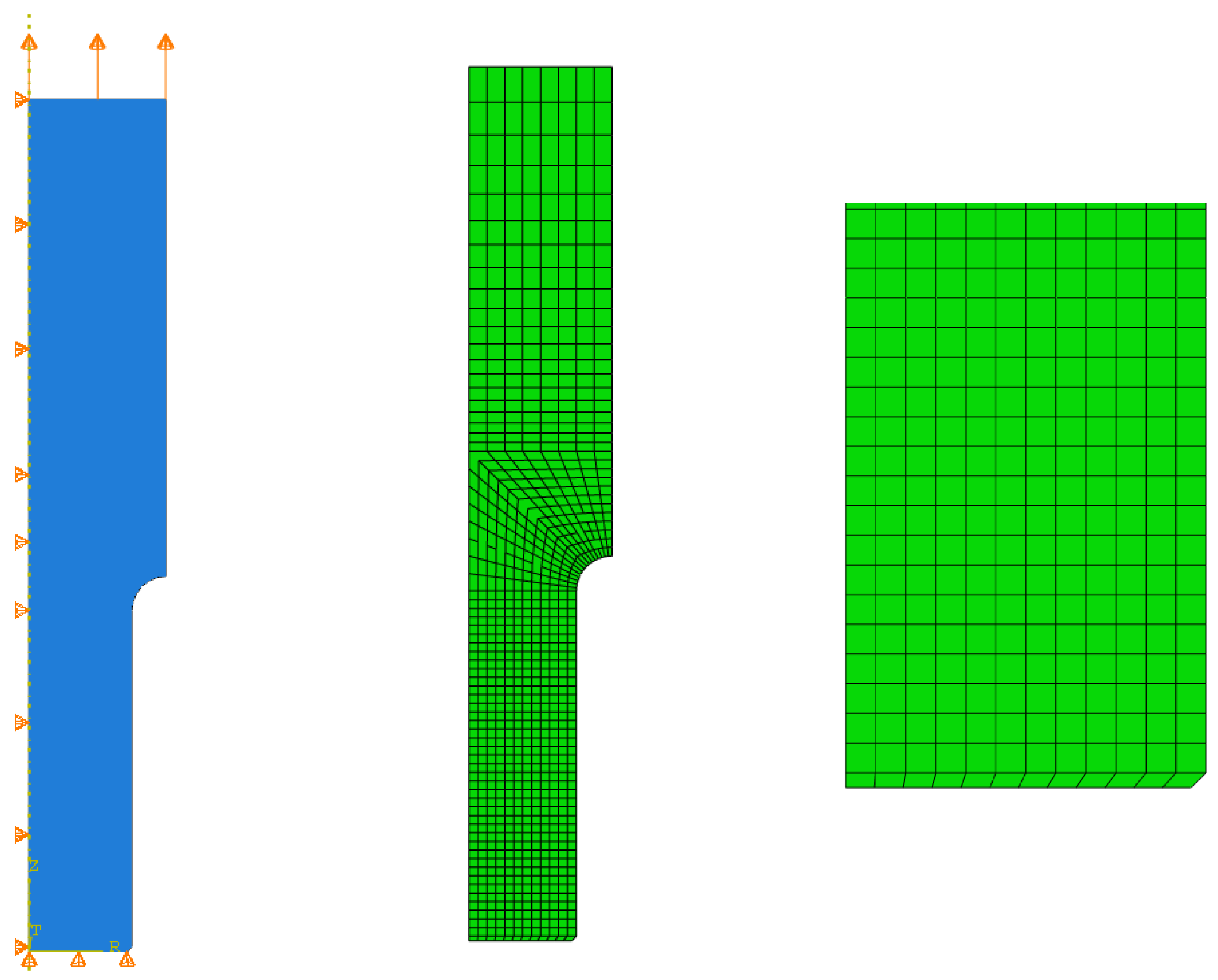
Figure 1 shows the geometry of the specimen. Because of the axisymmetric cross-section of the round bar, only one plain section of it was conducted. To ensure necking appears small notch made - it is a procedure well known from the literature [
45]. 844 quadrilateral FEM elements known in the ABAQUS system as CAX4R (4-node bilinear axisymmetric element). Reduced integration has been used in this case. As can be seen, the bottom part of the specimen was discretized with smaller FEM elements. The side of the brick element is 0.5 mm. The top part of the sample is divided using finite elements with different sizes. Close to the rounding in the middle of the height the basic finite element size is 1.0 x 1.0 mm and is elongated to 1.0 x 2.0 mm on the top. It should be mentioned that some FEM studies are based on a combination of triangular (close to the necking) and quadrilateral elements (the remaining parts of the specimen) [
15,
16].
Figure 2 shows kinematic boundary conditions applied to the material specimen. The vertical displacements of the bottom edge are equal to zero (u
2=0), whereas horizontal displacements u
1=0 for the left edge being the symmetry axes. Kinematic boundary conditions of the top edge have been provided as the extending load and are introduced here as u
2=5.0 mm. The full Newton incremental method has been proposed to model incremental behavior in this case, and for this purpose an initial increment size was assumed 0.001, the minimum equal to 0.0001 and the maximum allowed increment size was 1. Obviously, large displacements have been allowed in this case study. All numerical experiments with ABAQUS have been carried out in Polish national network PL-Grid and approximate time consumption of the single incremental solution was about 5.0 minutes.
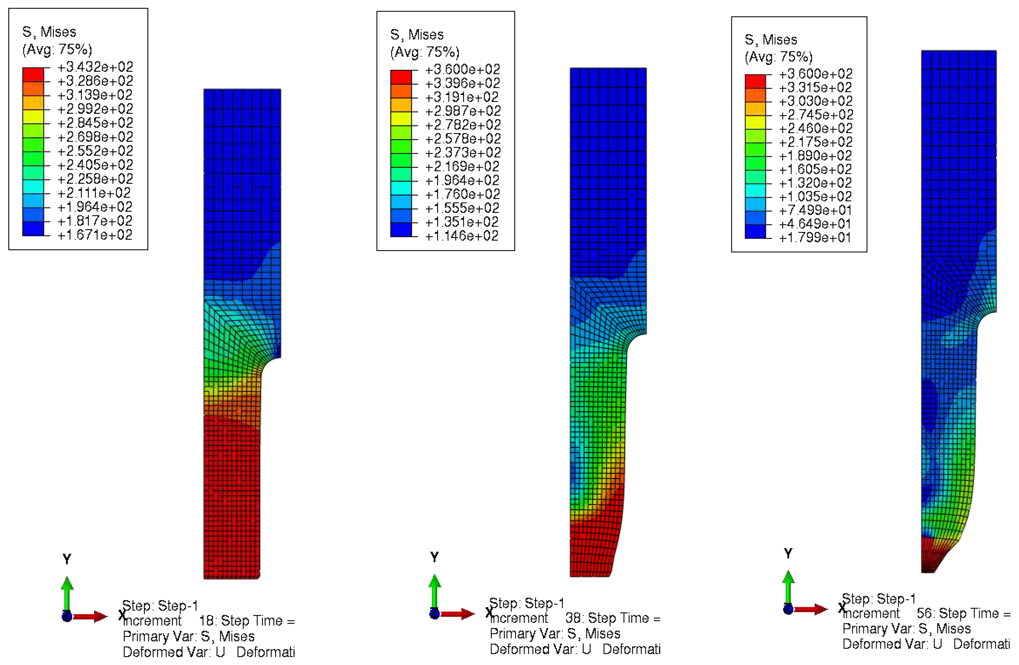
Figure 3 presents the resulting von Mises stress distribution in a few selected stages of the analysis (beginning, in the middle and at its end). After 20% of the analysis (left drawing) bottom part of the specimen has stress close to ultimate strength
fu=360 MPa here. After 50-60 percent of the analysis (middle drawing) necking occurs, and the reduced stress reaches maximum values of 360 MPa. At the end of the analysis, necking is fully developed and maximum stress is concentrated in the vicinity of this cross-section.
Further part of numerical simulation has been delivered in the computer algebra system MAPLE, where the LSM approximation together with the three chosen probabilistic methods have been programmed. Additionally, the final part of the FORM and relative entropy computations have been also prepared in the same system by the script developed by the Authors. Most of the results have been presented below as the functions of increasing uncertainty introduced in the model, so that deterministic solutions are obtained as the lower bounds for all of these characteristics and largest scattering is the upper bound on the windows containing up to the fourth order characteristics and entropies.
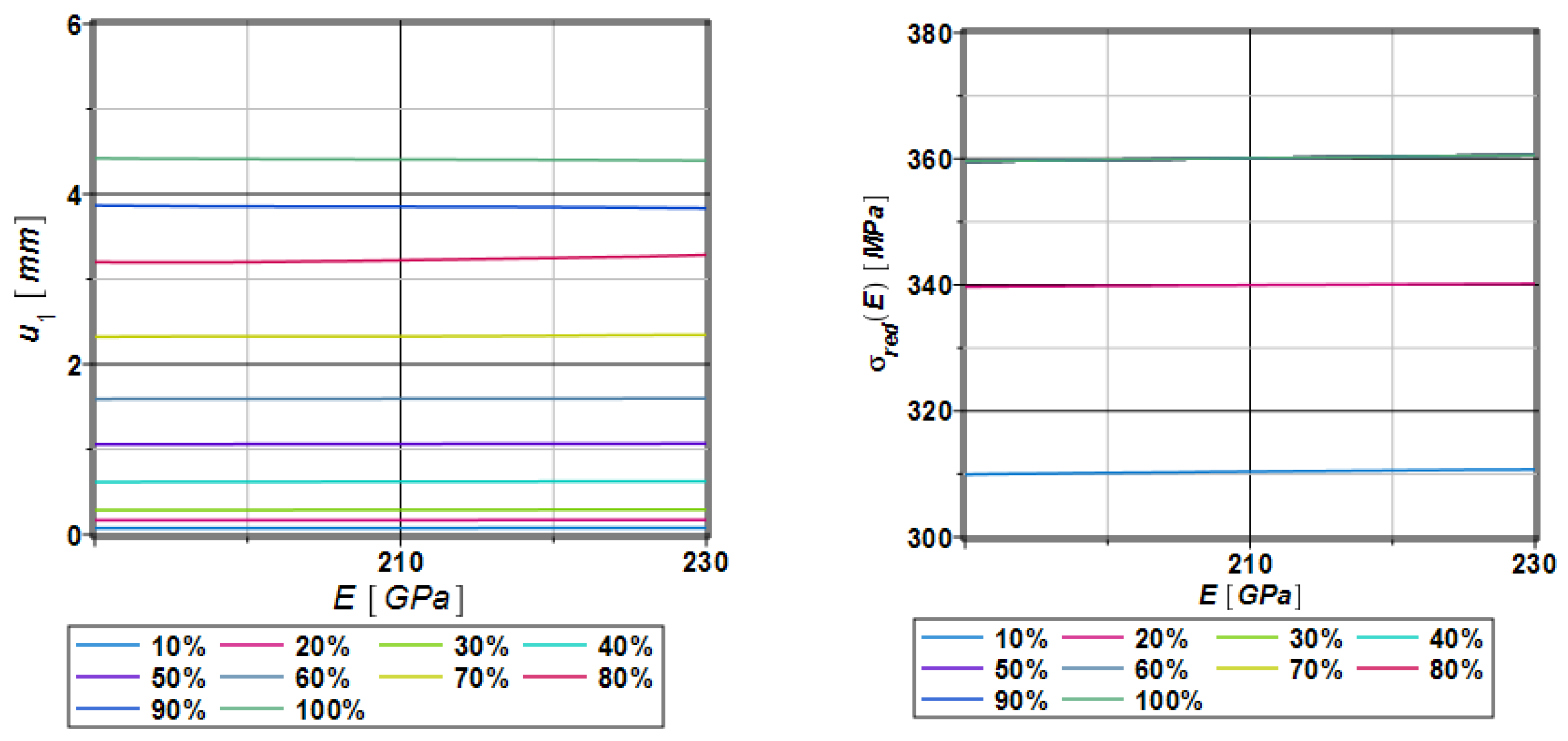
Figure 4 presents response function polynomials of displacements (left one) dependent on Young modulus values from range 190,…,210,...,230 GPa. Such a relatively small dispersion causes displacements that are independent of the Young modulus. Moreover, displacements are concentrated around its mean values. The right part of
Figure 4 shows response function method polynomials through the entire Young modulus dispersion, whereas shortly after about 30% of the analysis progress the resulting stress reaches maximum values 360 MPa. All the resulting polynomials are independent of the Young modulus. Further, this parameter is adopted as the main uncertainty source in our specimen, which follows a number of experimental works in civil engineering. Its mean value of 210 GPa has been further considered as the expected value, while the standard deviation has been adopted as 10% of this value, which agrees in many laboratory verifications. The second motivation for this choice is that this parameter is inherent in most of the civil engineering reliability studies as the design parameter, so it can be decisive for designing of most of more advanced structures, so that needs more attention.
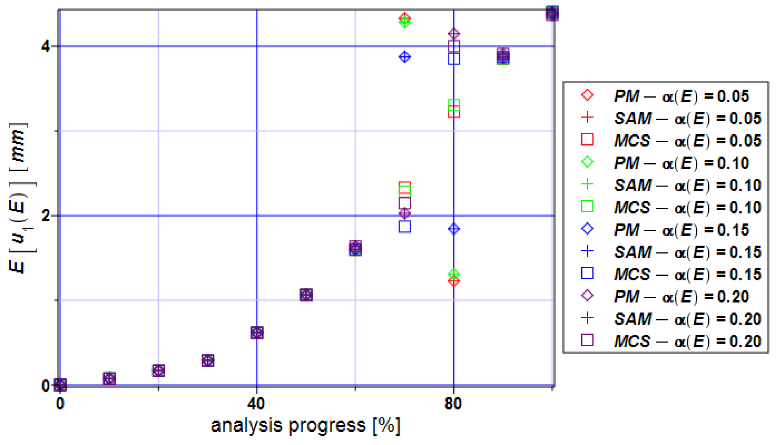
Figure 5 presents the distribution of the expectations of the extreme horizontal displacements as a function of the Young modulus E and those displacements follow the range of the necking. The perturbation method (PM), semi-analytical method (SAM), and Monte-Carlo Simulation (MCS) have been compared. At the beginning of the analysis, each method provides the same values of the necking concentrated round mean values. After about 70-80% of the process, some fluctuations can be observed. It can be identified with necking rapid expansion.
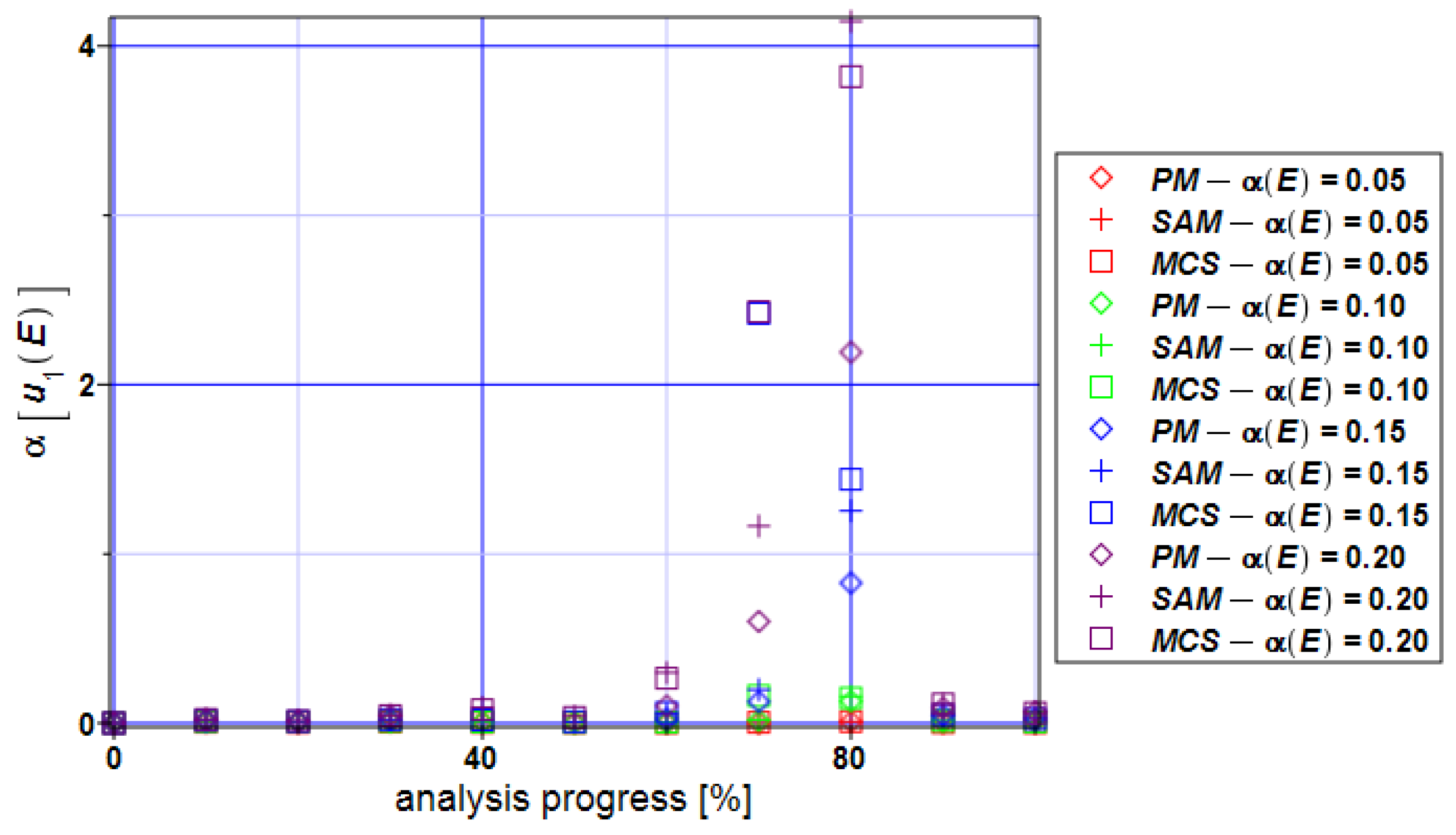
Figure 6 shows the coefficients of the variation of the maximum horizontal displacements. Numerical values of this coefficient keep close to the input value throughout the entire analysis except the extreme input uncertainty, which results in enormously large displacements statistical scattering (close to even 4, which never happens in elasticity). These extreme coefficient of variation are noticed for about 70-80% - the absolute extreme has been noticed while using semi-analytical method, a little bit smaller value has been detected with the use of the Monte-Carlo simulation, whereas the perturbation method results in the minimum extreme value here.
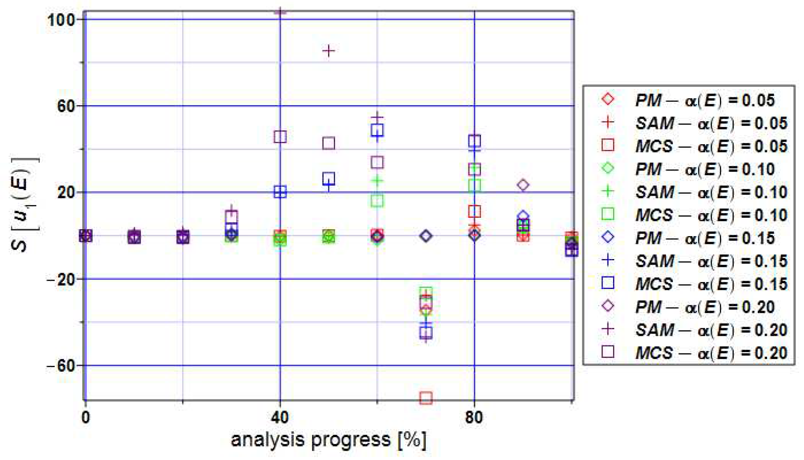
Figure 7 presents the distribution of skewness values throughout the entire numerical experiment. At the beginning of this analysis, it takes values close to zero which tells us about the symmetry of the distribution of this state function. Skewness takes both positive and negative values for all three methods but most of them are positive. It tells us about the left-skewed distribution of the displacement state function. Skewness according to the perturbation method is close to zero if we narrow input CoV α(E)<0.15.
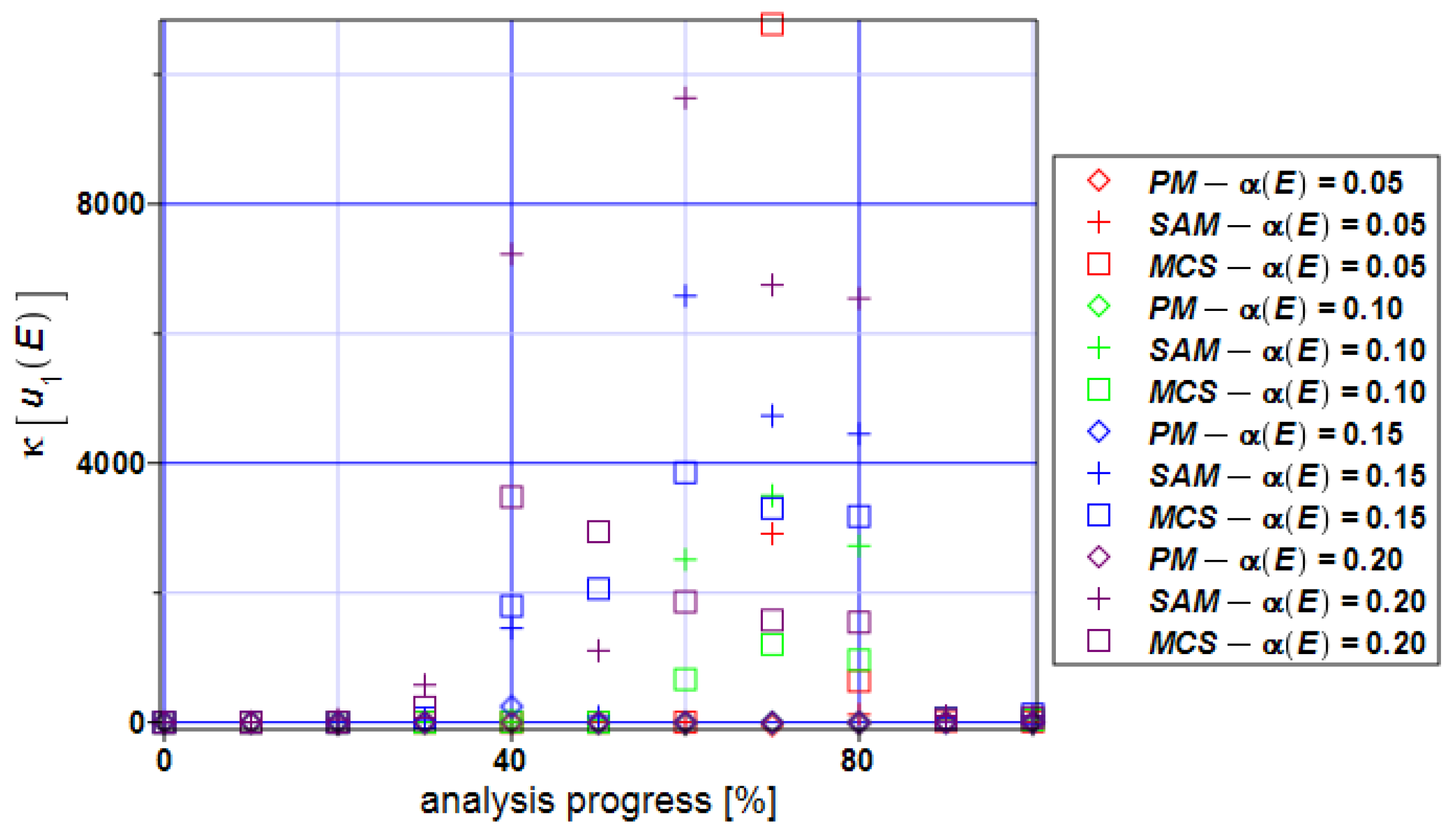
Kurtosis of the horizontal displacements of the specimen (
Figure 8) takes positive values according to all three methods. The perturbation method brings values of the kurtosis closest to zero. Semi-analytical method and Monte-Carlo Simulation take positive values of more than 2000 in the middle part of the analysis if α(E)>0.05. The biggest positive values kurtosis takes for Monte-Carlo Simulation for α(E)=0.05.
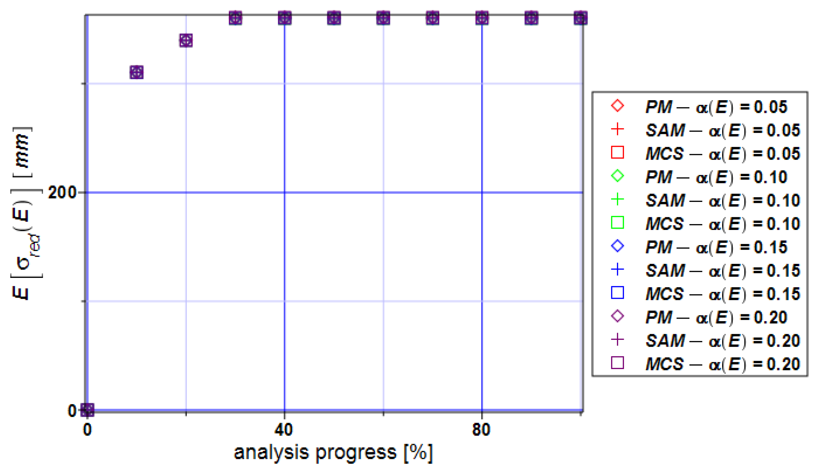
Figure 9 shows expectations of the von Mises reduced stress for the specimen. It can be seen that all three methods bring the same values which are very close to their means in a whole range of the input CoV α(E)=[0.05..0.20].
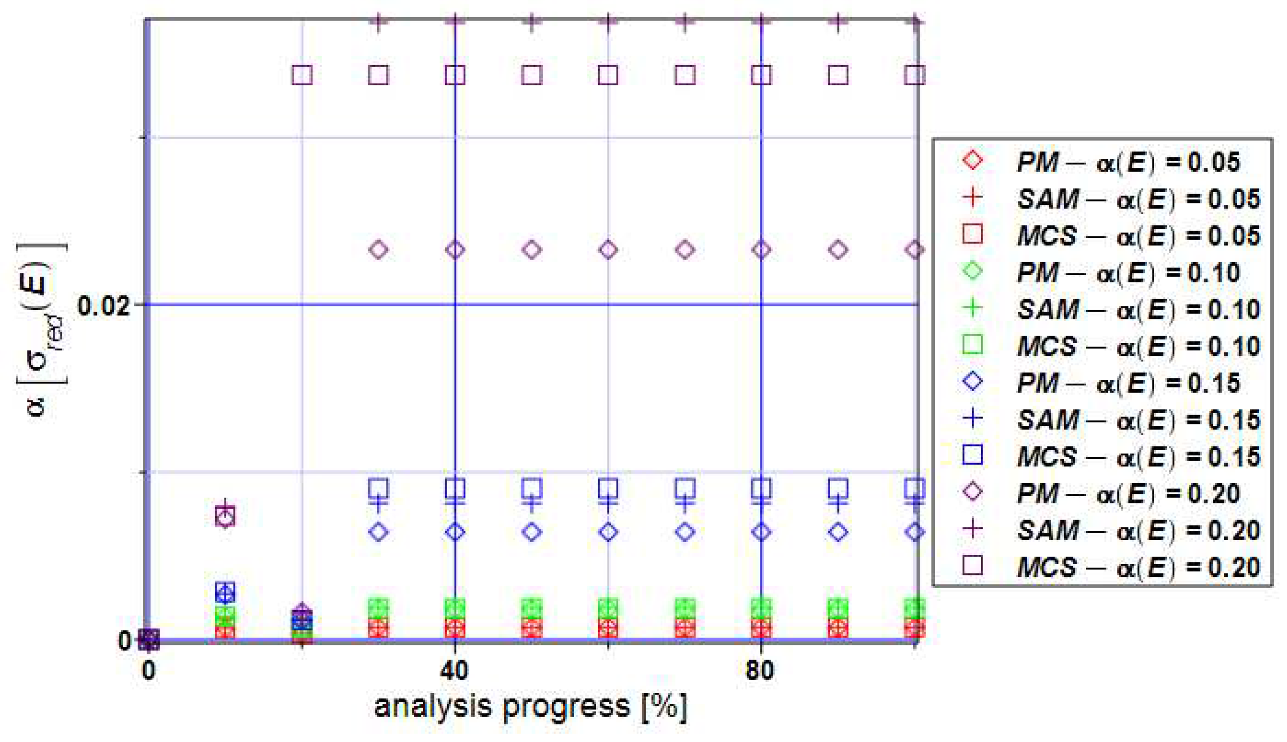
The coefficient of variation of the reduced stress (
Figure 10) is extremely close to zero based on all three methods. It means that expectations reflect mean values and this fact can be seen in
Figure 9. Practically no uncertainty is observed in the reduced stresses here while contrasting these results with the series from
Figure 6.
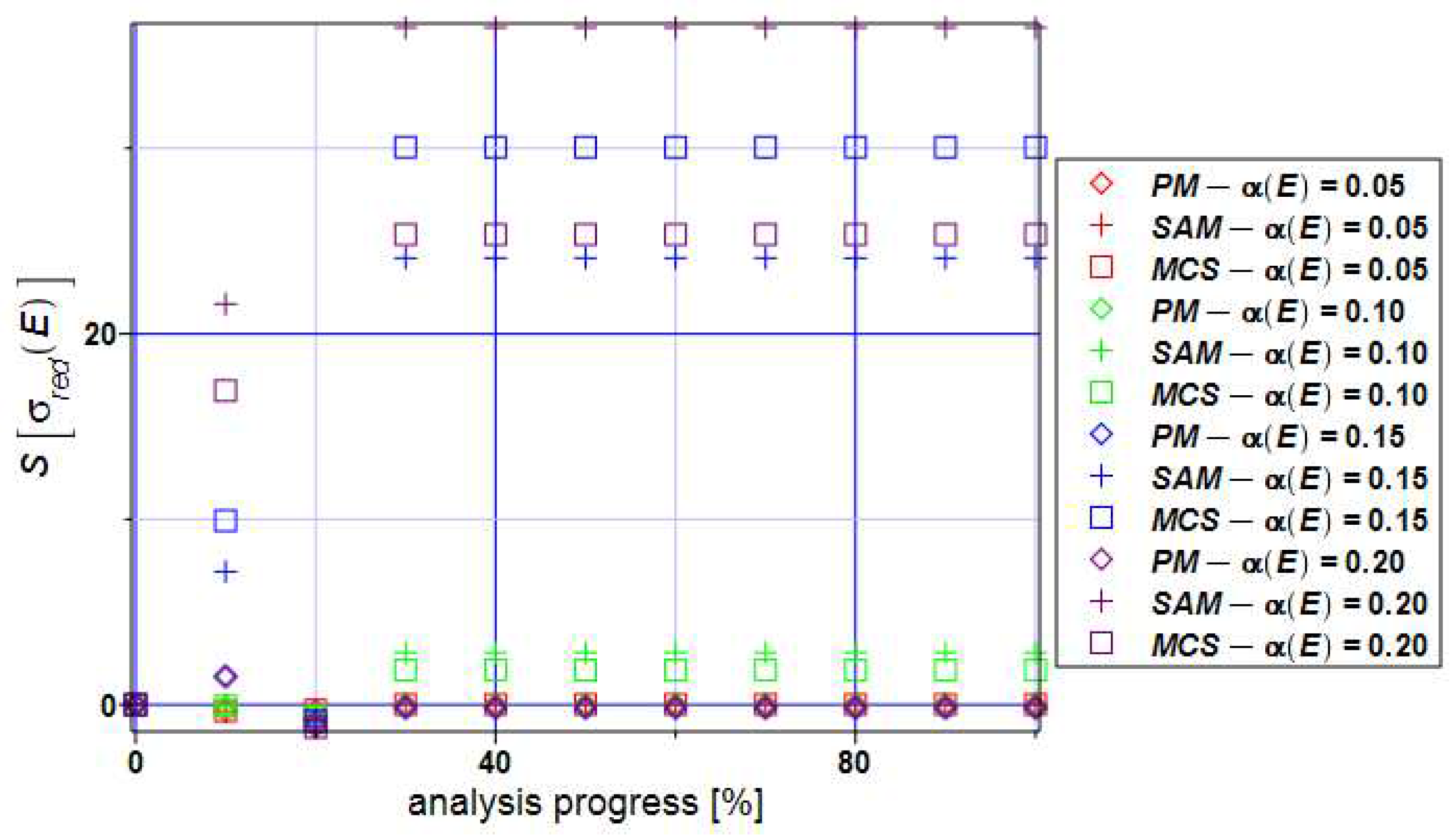
Skewness contained in
Figure 11 dominantly takes values close to zero if we limit the input coefficient of variation CoV to the values α(E)<0.10. Semi-analytical method and Monte-Carlo Simulation bring values larger than 20 for input CoV 0.15 and 0.20. Positive values of the skewness tell us that the distribution of von Mises reduced stress is left-skewed and should not be modelled using Gaussian PDF.
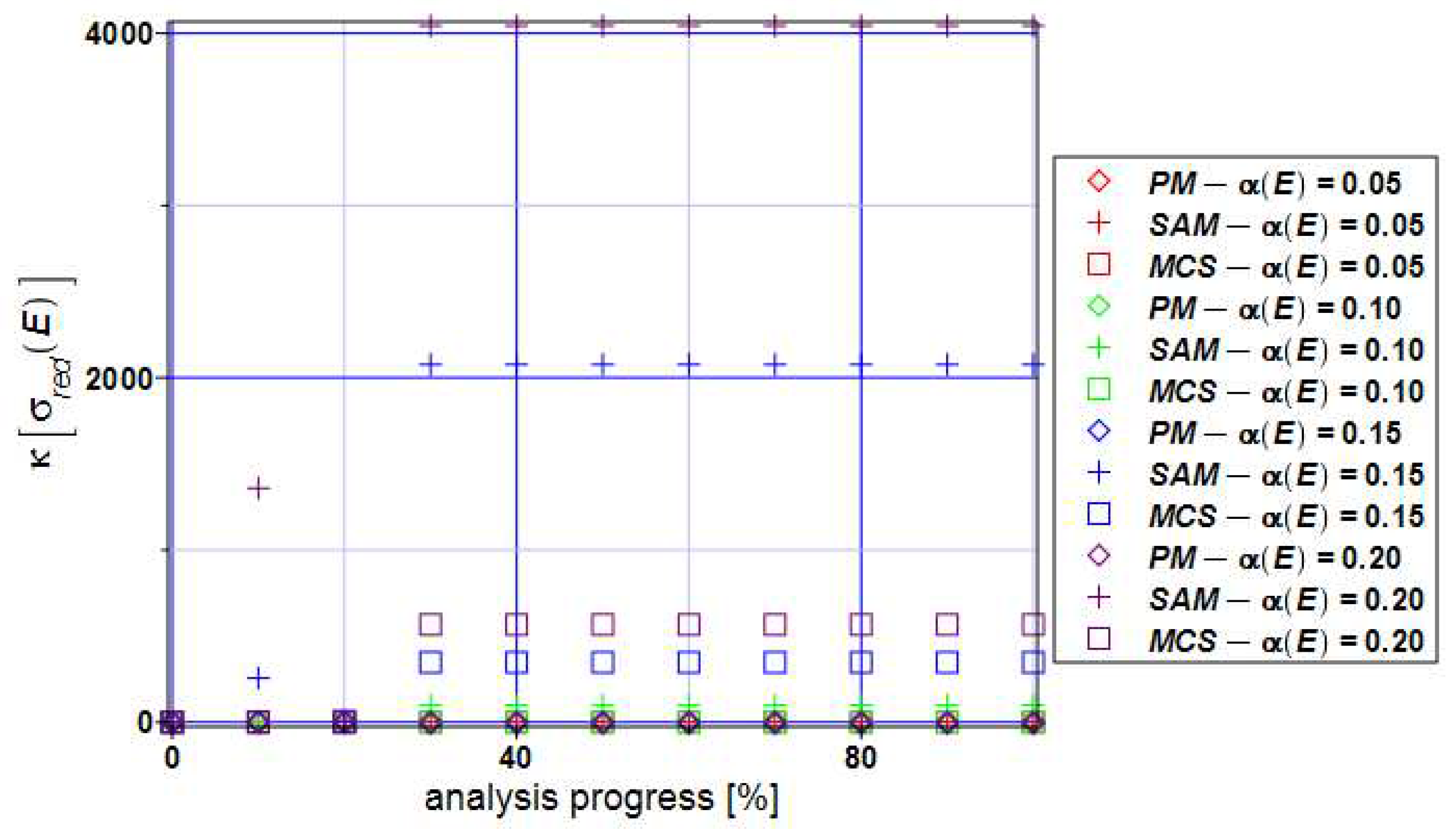
Kurtosis of the extreme reduced stress (
Figure 12) takes positive values throughout the entire extension process. Semi-analytical method and Mont-Carlo Simulation bring the values of the kurtosis in the range 2000-4000 for α(E)>0.10. It tells us that von Mises reduced stress distribution has long tails and peaks. If one bounds input CoV with α(E)≤0.05 then the distribution could be approximated by the Gaussian distribution with a relatively small modeling error.
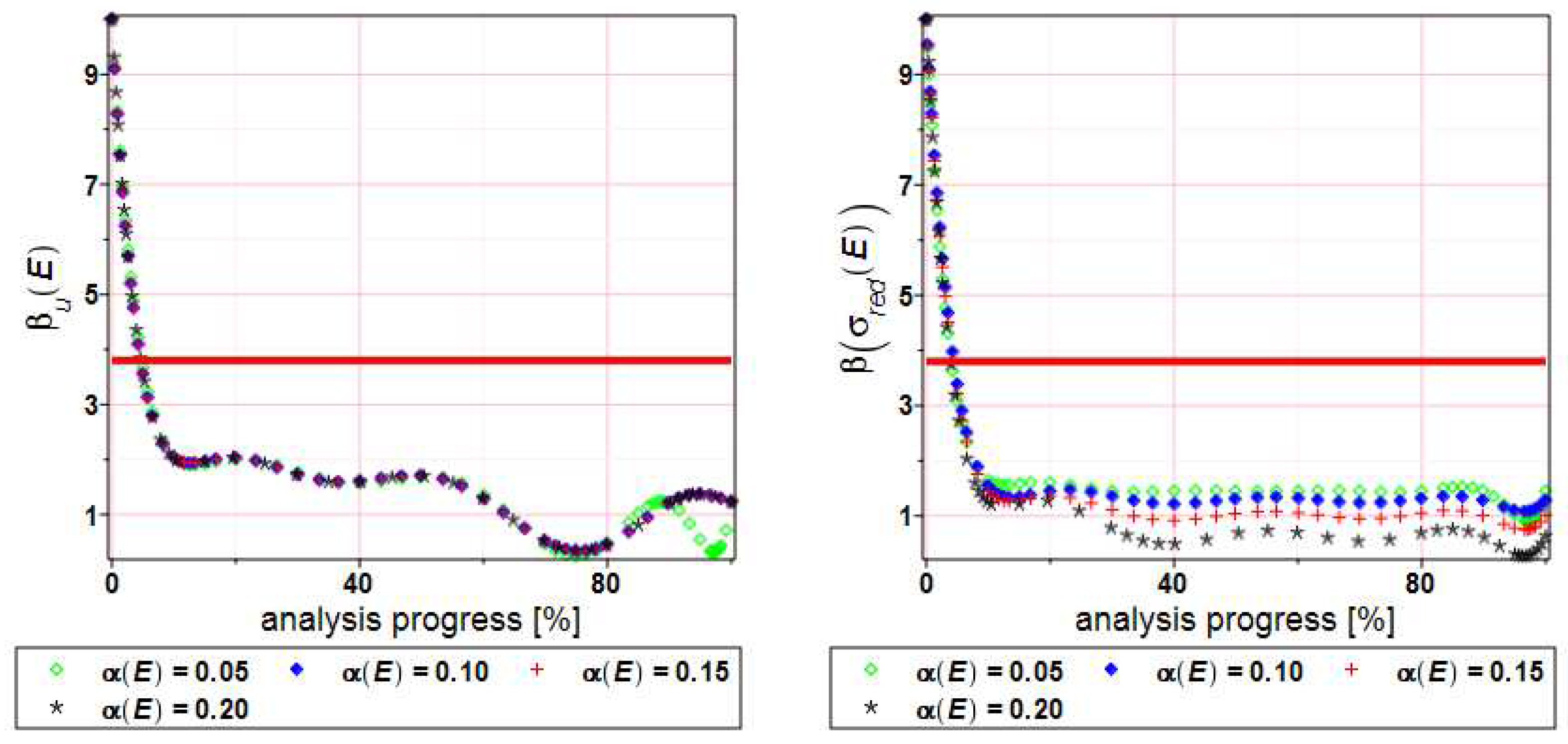
Figure 13 shows the reliability index distribution regarding displacements (left) and stress state (right). The red line is a safety level for normal, typical constructions. Reliability index β
u(E) takes the same values in a whole range of the input CoV. The amount of 90% of the specimen width has been taken as a limit value of the admissible extension (displacement). It is just an assumption because there is a complete lack of guidelines on how to calculate limit value. It can be observed that the specimen is in the failure region pretty fast (after 10 % of the analysis progress). But it relates to the expected values of the reduced stress (
Figure 9). The values equal to the ultimate strength 360 MPa can be noticed at the beginning of the process (after 30-40%), while the stress equal to 360 MPa persists to the same end of numerical analysis. The specimen is close to the breaking and that’s the reason why the reliability index takes values below the red line. One can see that the reliability index highly depends on the progress of nonlinear deformation, but it remains almost insensitive to the input CoV, α(E). Generally, bigger random dispersion in the specimen Young modulus leads to smaller values of the index β until its lowest admissible value is reached. Further, the reliability index decreases but in an oscillating manner, and below the red limit we may observe some differences obtained for various statistical scattering in the input Young modulus.
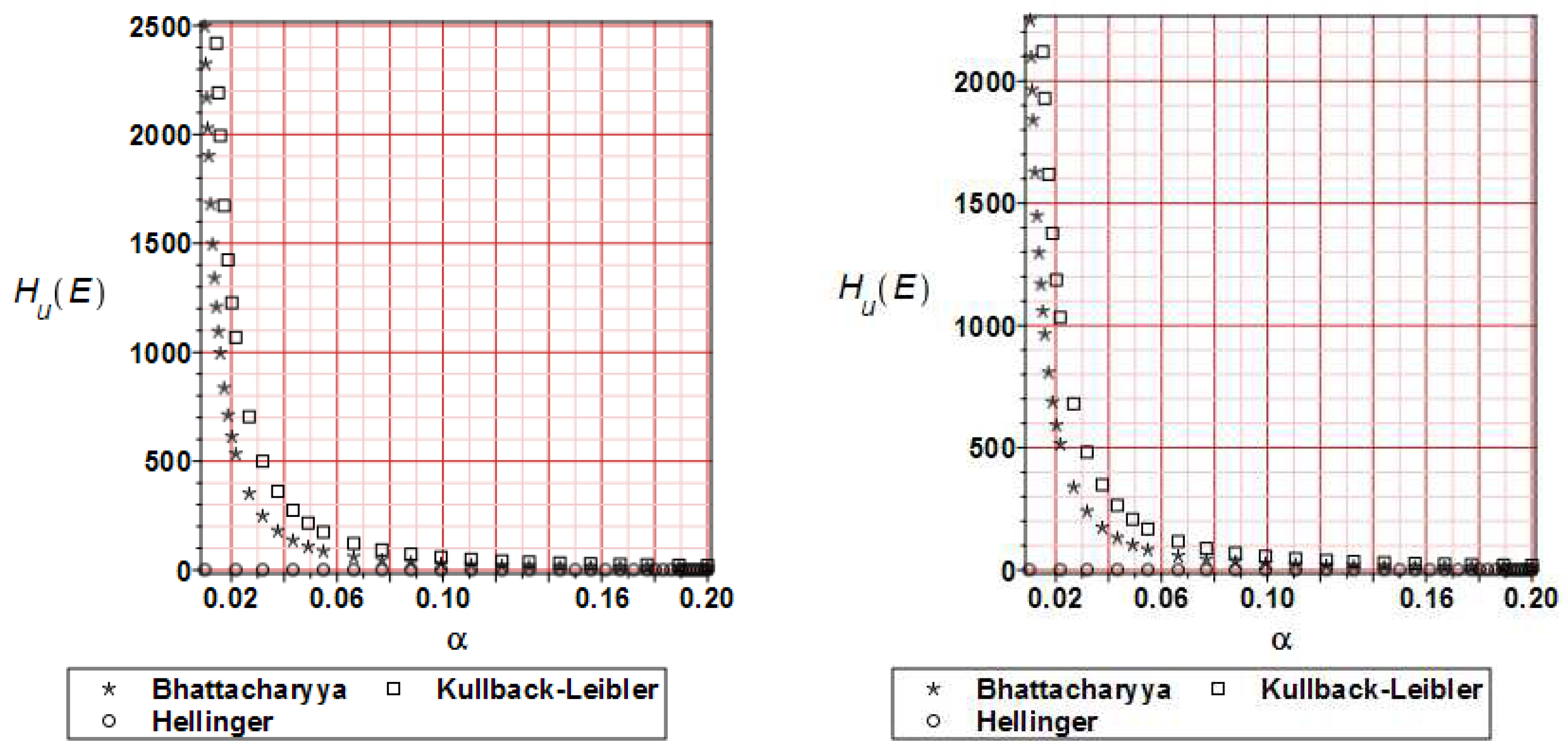
Figure 14 shows the relative entropy distribution for the horizontal displacements, where the input CoV has been taken from the interval α=[0..0.20], as before. The few relative entropies models developed by Bhattacharyya, Kullback-Leibler and Hellinger’s have been compared with each other. During the entire analysis, the first two methods bring similar results. In the beginning, entropy reaches the values over 2500 for α<0.02. Then it decreases to minimum values at the end of the analysis. It has to be underlined that Hellinger equations provide smaller values of the relative entropy keeping close to 0 within the entire variability interval of the parameter α, and therefore, this relative entropy model seems to be less useful in reliability assessment.
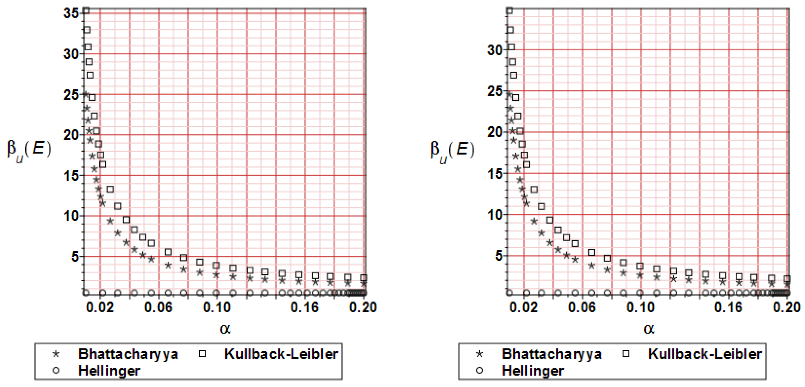
Figure 15 presents the reliability index distribution for the displacements calculated based on relative entropy values; the nature of the curves is similar to
Figure 14 but values are proportionally smaller. Compared with
Figure 13 (left) it can be observed that the reliability index takes values 4-5 times bigger than the original relative entropy. All the curves behave in the way typical for classical reliability indices – they exponentially decrease while increasing analysis progress. A remarkable difference to the left graph of
Figure 13 is that now reliability indices have remarkably larger values, so that the FORM approach returns less favorable values. Bhattacharyya model returns slightly smaller values than the Kullback-Leibler trend, while Hellinger model keeps almost constant and close to the interval [0, 1].
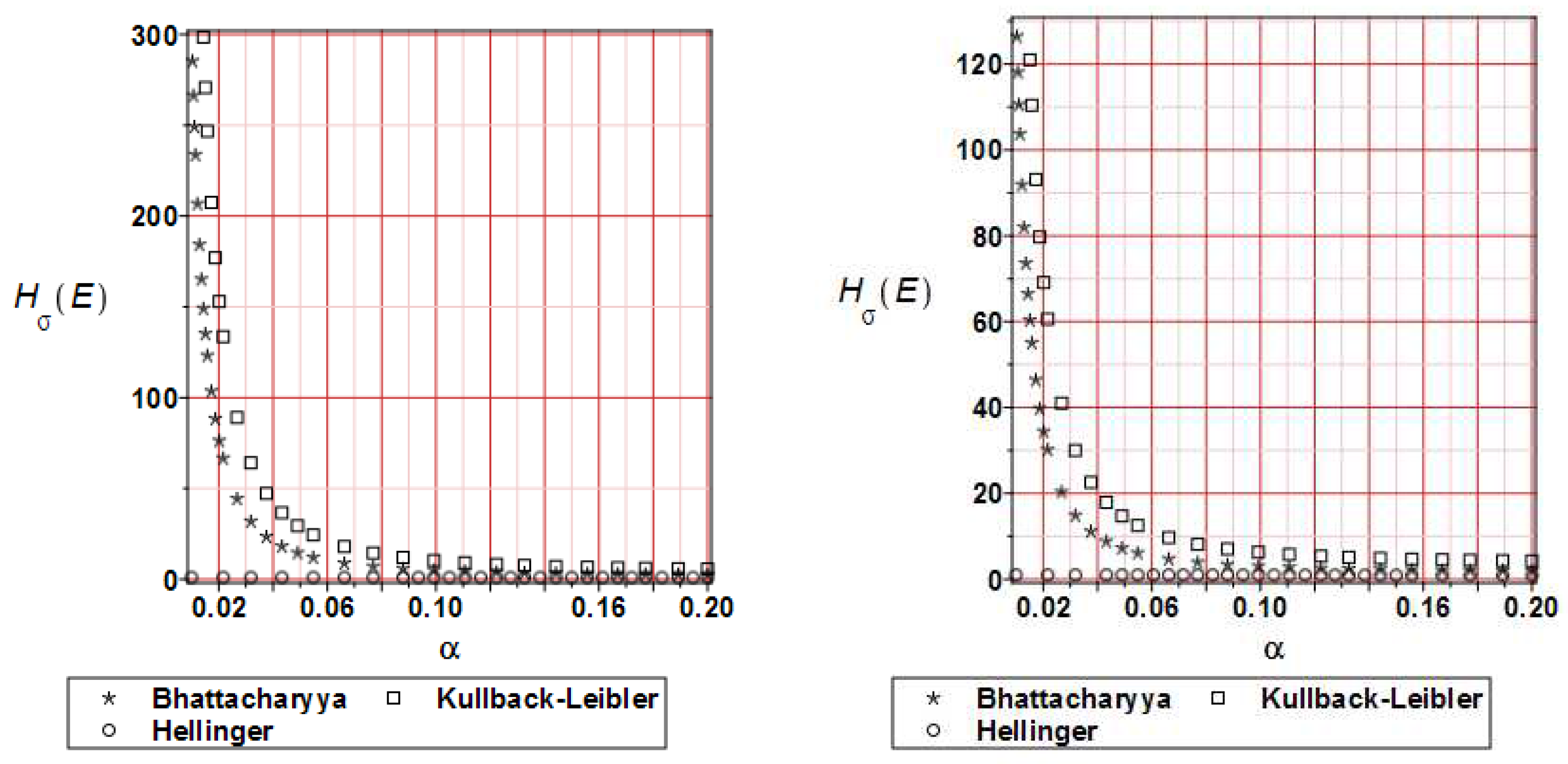
The distribution of the relative entropy for the reduced stress H
σ(E) after 20 and 80 % of the analysis progress is presented in
Figure 16. The most popular methods have been compared. As was observed for displacements Bhattacharyya and Kullback-Leibler methods bring similar character to the graphs; larger input CoV causes remarkable reduction of the entropy values. Hellinger’s method leads to values close to zero throughout the entire analysis.
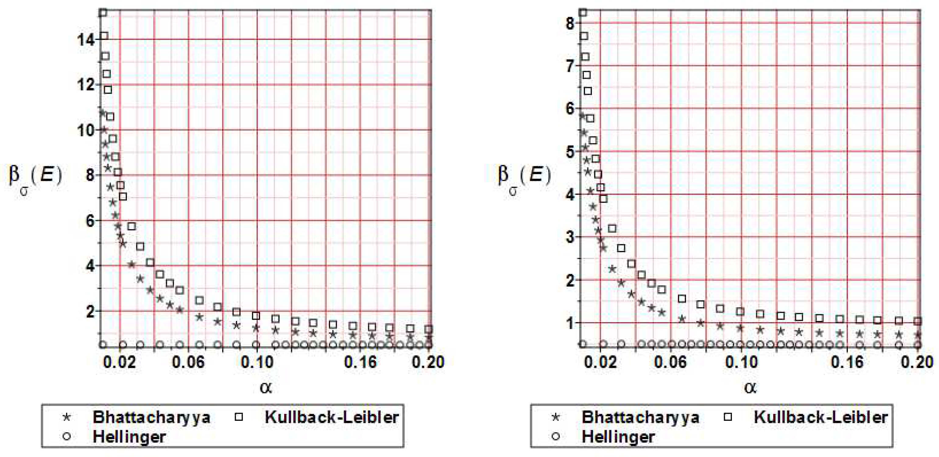
Figure 17 shows the reliability index distribution for the reduced stress; it is based on the relative entropy course. All the curves are similar to relative entropy distribution with this note that the reliability index takes 10-15 times smaller values. Quite interestingly, their numerical values are close to numerical values obtained in the right graph of
Figure 13, where the FORM reliability indices for the ULS have been presented. One may even notice that all of these trends return less favorable reliability estimation than the FORM analysis. It is seen that a difference in Kullback-Leibler model to the FORM curve is the smallest one, whereas Hellinger relative entropy returns once more less useful results because its reliability based index is less than 1. As one could expect, which agrees with engineering intuition, the reliability index based on the relative entropy remarkably decrease together with deformation process. It is obvious that probability of failure must increase while approaching to the end of numerical simulation and it is numerically proven here.
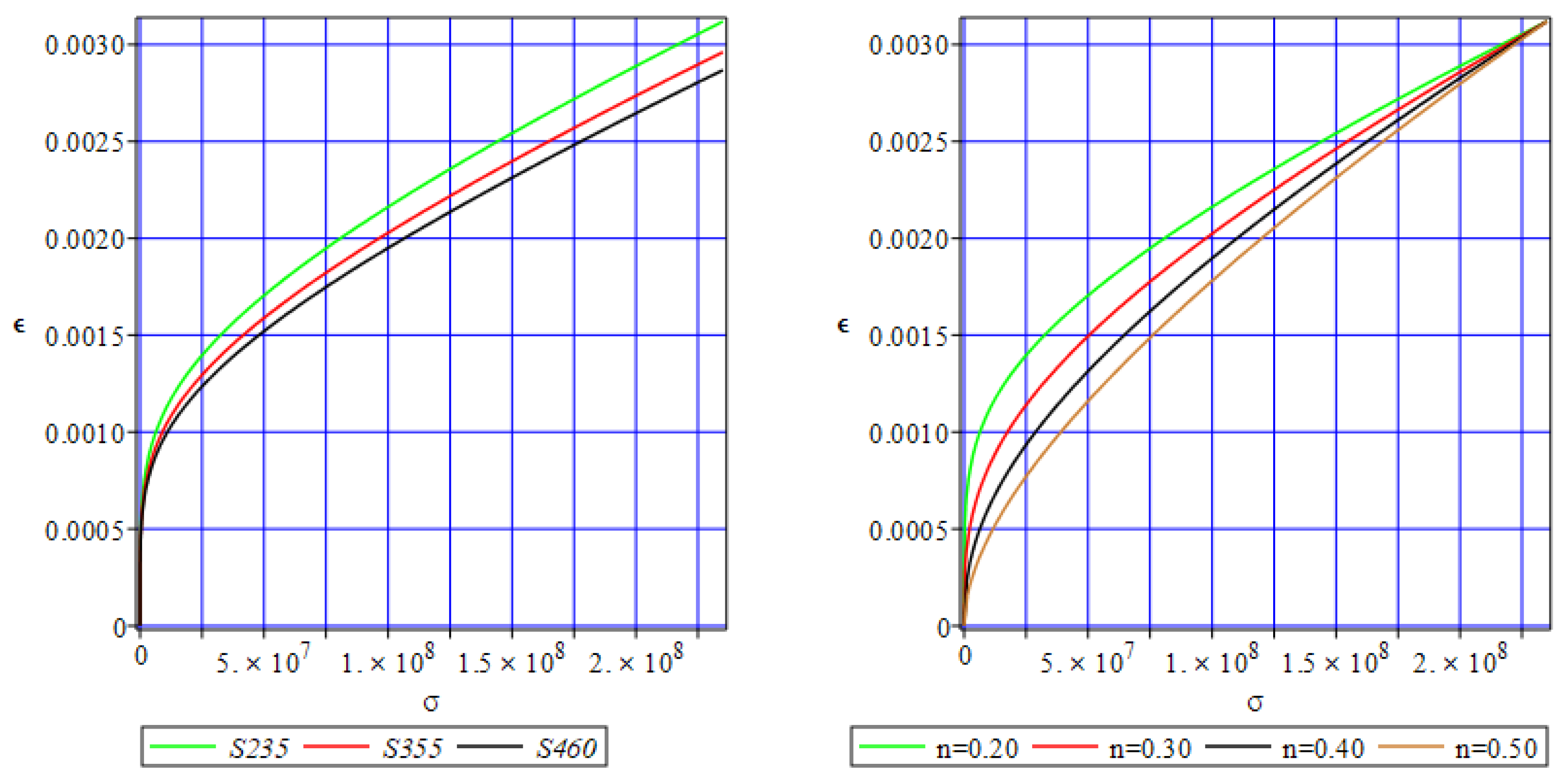
Figure 1.
Stress-strain curves according to Ramberg-Osgood law for different structural steels (left) and sensitivity of S235 to the strain hardening coefficient (right).
Figure 1.
Stress-strain curves according to Ramberg-Osgood law for different structural steels (left) and sensitivity of S235 to the strain hardening coefficient (right).
Figure 2.
Geometry, boundary conditions, and meshing of the specimen.
Figure 2.
Geometry, boundary conditions, and meshing of the specimen.
Figure 3.
Resulting von Mises stress distribution for 20, 60, and 100% of the analysis progress.
Figure 3.
Resulting von Mises stress distribution for 20, 60, and 100% of the analysis progress.
Figure 4.
Response function polynomials of displacements and reduced stress as a function of the Young modulus E.
Figure 4.
Response function polynomials of displacements and reduced stress as a function of the Young modulus E.
Figure 5.
Expectations of the extreme displacements E[u1(E)] for the specimen.
Figure 5.
Expectations of the extreme displacements E[u1(E)] for the specimen.
Figure 6.
Coefficients of variation of the extreme displacements α[u1(E)] for the specimen.
Figure 6.
Coefficients of variation of the extreme displacements α[u1(E)] for the specimen.
Figure 7.
Skewness of the extreme displacements S[u1(E)] for the specimen.
Figure 7.
Skewness of the extreme displacements S[u1(E)] for the specimen.
Figure 8.
Kurtosis of the extreme displacements κ[u1(E)] for the specimen.
Figure 8.
Kurtosis of the extreme displacements κ[u1(E)] for the specimen.
Figure 9.
Expectations of the extreme reduced stress E[σ(E)] for the specimen.
Figure 9.
Expectations of the extreme reduced stress E[σ(E)] for the specimen.
Figure 10.
Coefficient of variation of the extreme reduced stress α[σ(E)] for the specimen.
Figure 10.
Coefficient of variation of the extreme reduced stress α[σ(E)] for the specimen.
Figure 11.
Skewness of the extreme reduced stress S[σ(E)] for the specimen.
Figure 11.
Skewness of the extreme reduced stress S[σ(E)] for the specimen.
Figure 12.
Kurtosis of the extreme reduced stress κ[σ(E)] for the specimen.
Figure 12.
Kurtosis of the extreme reduced stress κ[σ(E)] for the specimen.
Figure 13.
Reliability index of the displacements βu(E) and extreme reduced stress β[σ(E)] for the specimen.
Figure 13.
Reliability index of the displacements βu(E) and extreme reduced stress β[σ(E)] for the specimen.
Figure 14.
Relative entropy comparison for the displacements Hu(E) at 20 and 80 % of the analysis progress.
Figure 14.
Relative entropy comparison for the displacements Hu(E) at 20 and 80 % of the analysis progress.
Figure 15.
Reliability index βu(E) comparison for the displacements at 20 and 80 % of the analysis progress.
Figure 15.
Reliability index βu(E) comparison for the displacements at 20 and 80 % of the analysis progress.
Figure 16.
Relative entropy comparison for the reduced stress Hσ(E) at 20 and 80 % of the analysis progress.
Figure 16.
Relative entropy comparison for the reduced stress Hσ(E) at 20 and 80 % of the analysis progress.
Figure 17.
Reliability index βσ(E) comparison for the reduced stress at 20 and 80% of the analysis progress.
Figure 17.
Reliability index βσ(E) comparison for the reduced stress at 20 and 80% of the analysis progress.
