Meteorological Signal on Hydrodynamics in the Ilha Grande and Sepetiba Bays: Lag Effects and Coastal Currents

In the southeastern coast of Brazil, the bays of Ilha Grande and Sepetiba are linked by the Ilha Grande Channel, where remarkably vigorous currents have been consistently observed. The sheer intensity of these currents defies a simple explanation through tidal forcing alone, prompting researchers to delve into potential influences such as basin resonance and the baroclinic effect. This study aims to elucidate the role of remote meteorological effects within this complex hydrodynamic system. A numerical approach with a coastal model nested within an ocean model was employed, enabling an in-depth examination of the intricate interplay between meteorological and tidal forcings. The study revealed a significant finding: the lag in signal propagation plays a pivotal role in determining how these signals impact the dynamics of the bays. The astronomical signal exhibits a minimal lag along the coast (1 minute), and leads to water level differences between the sea and the coastline, resulting in the generation of tidal currents at the bay entrances. On the other hand, the remote meteorological signal, with a stronger signal lag along the coast (4.92 hours), leads to the creation of water level difference between the bay’s entrances, inducing significant fluxes along the narrow Ilha Grande Channel.

Keywords:

Subject: Environmental and Earth Sciences - Oceanography

1. Introduction

The coastal region represents a dynamic interface where terrestrial, marine, and atmospheric systems intersect, and where the actions of humans not only impact the coastal area but are also influenced by the integrated behavior of these three interconnected domains. This unique setting is vulnerable to various hazards, including erosion, subsidence, tsunamis, and flooding, all of which can be exacerbated by rising sea levels and river floods [1]. Moreover, when astronomical and meteorological factors combine, they can give rise to extreme sea level events, which pose a substantial threat to coastal communities and ecosystems, as well as the destruction of critical port and coastal structures [2]. As noted by Mestres et al., 2016, port authorities have increasingly focused on this phenomenon due to its potential to impede the safe maneuvering, approach, and entry of ships into ports, thus posing a risk of accidents. This combination of factors has been a significant contributor to disasters, as reported by the World Meteorological Organization [3], accounting for 44% of recorded disasters and 31% of economic losses between 1970 and 2019. It underscores the urgent need for comprehensive understanding and management of coastal dynamics to mitigate these risks effectively.

Sea level temporal variation (η(t)) can be written as Pugh [4]:

η (t) = η_{0} (t) + η_{A} (t) + η_{M} (t)

(1)

Slow Variations in Time η₀(t): This component accounts for gradual changes in sea level over time and can often be approximated by averaging for shorter time scales. It encompasses interannual and long-term variability, which are linked to eustatic (global sea level changes) and isostatic (crustal adjustments) processes.

Astronomical Component η_A(t): The astronomical component of sea level variation primarily arises from tidal generating forces, as indicated by research by Bowden [5] and Open University [6]. Tides, in general, constitute the predominant driver of sea level fluctuations along coastlines, as emphasized by Pugh [4].

Meteorological Component η_M(t): The meteorological component represents the difference between the observed sea level and the astronomical signal, as described by Marone and Camargo [7] and Pugh [4]. This component captures the influence of meteorological factors on sea level. Importantly, Marone and Camargo [7] note that only about 10% of this residual signal is typically attributed to changes in atmospheric pressure, while the majority is associated with wind-induced friction on the sea surface. This wind-induced friction can generate oscillations in sea level, which can originate either locally or remotely.

These oscillations may occur as Coastal Trapped Waves (CTW), which are categorized into two main types: Supra-inertial Waves (Edge Waves): These CTW occur at frequencies higher than the Earth's inertial frequency. They can be excited by various meteorological forcings, including changes in atmospheric pressure (inverted barometer effect), wind wave radiation in shallow water, and wave refraction and diffraction effects. These forcings typically have a localized impact on water level [4,7]. Subinertial Waves: These CTW occur at frequencies lower than the Earth's inertial frequency and are primarily associated with remote origins [4]. The Ekman transport associated with wind parallel to the coast can generate these subinertial waves. It results in an oscillatory motion that remains trapped along the coast through geostrophic balance balance [8,9] with a cyclonic direction of propagation. These waves carry energy from the wind-affected area to other coastal regions [10]. These subinertial oscillations are influenced by Earth's rotation [11], with the Coriolis Force acting as a restoring mechanism.

In summary, sea level variation is a multifaceted phenomenon shaped by slow temporal changes, astronomical forces (primarily tides), and meteorological factors (especially wind-induced effects), where Coastal Trapped Waves play a crucial role in understanding the complex dynamics of coastal sea level fluctuations.

The term "storm surges," as defined by Idier et al. [12], refers to long waves that arise from changes in atmospheric pressure and the stress of wind on the sea surface. These waves propagate along coastlines as shallow water waves and are subject to various influences, including bottom friction, the Earth's rotation (Coriolis force), and local amplifications due to resonant effects.

Wang and Elliott [13] conducted a study on estuarine circulation in the Chesapeake Bay and observed that most of the non-tidal fluctuations occur on seasonal and storm time scales. They also noted that during certain periods, remote wind forcing dominates over local effects, underscoring the importance of considering both factors in estuarine circulation modeling. While local wind patterns play a prominent role in the upper estuary, affecting the slope between high and low estuary water levels, remote forcings impact the lower estuary, propagating as long waves into bays with minimal dissipation or amplification [14,15].

Melo Filho [16] discusses two approaches for simulating the remote wind effect. The first approach involves statistical methods, such as cross-correlation, linear regression models (as used by Truccolo et al. [17]), or neural network models (as employed by Oliveira et al. [18]). These statistical models rely on extensive databases to establish relationships between wind and water level changes. The second approach involves coupling coastal and oceanic numerical models using the nesting technique. In this way, coastal models simulate local hydrodynamics taking the effect of large and mesoscale oceanic and atmospheric circulation into account. In numerical coastal studies, is common ocean models provide boundary conditions for coastal models through grid nesting, as demonstrated by various studies [15,19,20,21]. This approach allows for a more comprehensive representation of the complex interactions between remote and local factors in coastal areas and their impact on estuarine circulation.

The southern and southeastern coast of Brazil falls under the influence of low-pressure frontal systems that interact with the western branch of the South Atlantic high-pressure system. The cold fronts linked to these low-pressure systems exhibit a seasonal pattern, being more frequent in Brazil during the austral autumn and winter [2], leading to shifts in wind direction. According to Veleda et al. [22], the combination of wind friction and the abrupt changes in coastline orientation between 22º S and 36º S along the Brazilian coast make this region particularly prone to generating Coastal Trapped Waves (CTW).

The irregularities in the bathymetry of the continental shelf result in alterations in the characteristics of CTW, including a decrease in propagation speed and amplitude [10,23]. Freitas et al. [24] suggest that this is evident along the southeastern Brazilian coast, where a decrease in CTW energy and phase speed propagation is observed towards the northern limit (around 22º S, between Tubarão Bight and Abrolhos Bank). This region features abrupt variations in the width and depth of the continental shelf.

Several studies, including Sandstrom [25], Truccolo et al. [17] and Andrade et al. [2], have emphasized the significance of the non-astronomical signal on sea level caused by CTW along the south and southeastern Brazilian coast. Meteorological events, particularly wind changes resulting from cold fronts along the southeastern Brazilian coast, can induce water level variations of a magnitude comparable to tidal effects [26]. Andrade et al. [2] conducted data analysis on the Rio Grande do Sul coast, revealing an average tidal variation of 0.30 meters. However, when the tidal signal was excluded, the water level signal reached up to 0.40 meters, underscoring the critical importance of studying the non-astronomical signal in this coastal area.

The study by Castro and Lee [27] conducted on the south-southeast Brazilian continental shelf revealed that sea level fluctuations exhibit periods ranging from 9 to 12 days and from 6 to 7 days. These fluctuations were found to be closely correlated with southern winds that occurred before the passage of these oscillations. Additionally, the presence of coastal trapped waves, was reported in the same area by França [28]. These waves are responsible for a significant portion of the energy propagated at subinertial frequencies towards the north, potentially leading to variations in current intensity within the subinertial band [29]. Considering the latitude where Sepetiba and Ilha Grande Bays are situated, the Earth's rotation imposes an approximate inertial period of more than 30.7 hours.

Melo Filho [7] conducted a study indicating that the variance of the subinertial signal associated with remote winds (with periods ranging between 3 to 30 days) along the Rio de Janeiro coast represents 66.0% of the total variance. Seasonality (periods ranging between 30 days and one year) accounts for 28.2%, while local winds (with periods ranging between 2 hours and 3 days) contribute 5.8%. Similar findings were reported by Rodrigues et al. [30], who found that 67.5% of the total signal variance corresponds to the subinertial along-channel currents component, featuring periods ranging from 2 to 30 days. Melo Filho [7] also noted that 50% of the meteorological influence in Rio de Janeiro originates from the area south of Imbituba, while 30% arises from the region between Imbituba and Rio de Janeiro.

The significance of flows related to various forces has been widely acknowledged in studies, including factors such as local wind friction and density [31,32,33]. However, as noted by Kjerfve et al. [34], for the Ilha Grande Channel, wind and ocean dynamics take on a paramount role in local hydrodynamics, accounting for 67% of the annual variation in sea level. In contrast, atmospheric pressure explains 5% of the annual sea level variation, while steric changes associated with shifts in temperature and salinity within the water column contribute to the remaining 28%.

Fragoso [35] observed an increase in current intensity in the Ilha Grande Channel, reaching up to 0.4 meters per second (more than 65%), attributed to meteorological effects. Cavalcante [36] associated currents with meteorological forcing, with intensities reaching around 0.4 meters per second in Ilha Grande Bay, approximately 0.05 meters per second in Sepetiba Bay, and up to 0.6 meters per second in the Ilha Grande Channel.

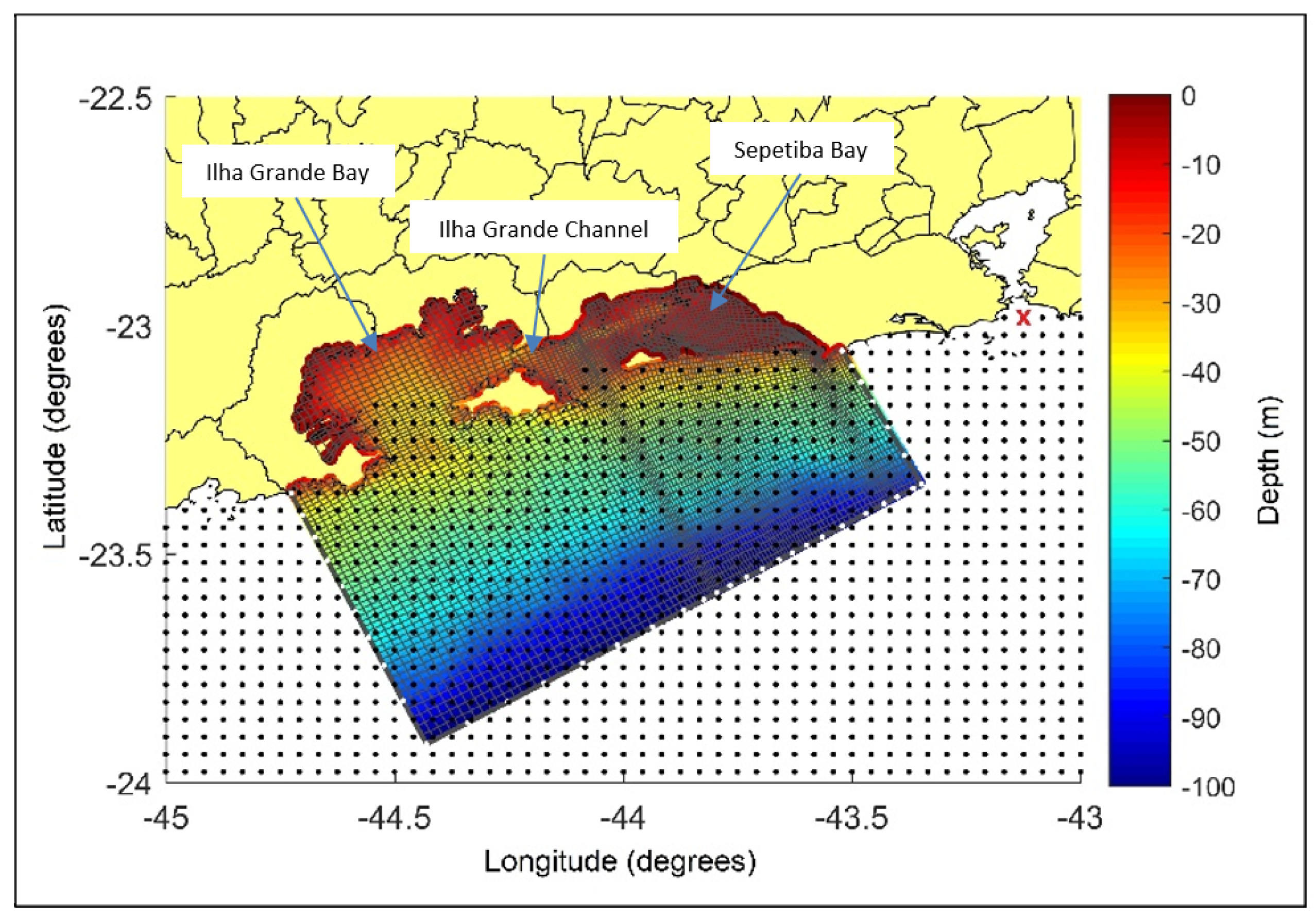
The primary objective of this study is to comprehend the role of the remote meteorological signal in intensifying currents within the Ilha Grande Channel (Figure 1). To achieve this objective, the research will investigate the patterns of both the remote meteorological signal and tides within Sepetiba and Ilha Grande Bays using a coastal model nested within an ocean model.

2. Materials and Methods

2.1. Study Area

The study area encompasses the complex of Sepetiba and Ilha Grande bays, situated on the southeastern coast of Brazil (see Figure 1) Sepetiba Bay is characterized by a intensive port activity, notably hosting the Port of Itaguaí, which ranks as the second-largest Brazilian port in terms of cargo flow [37]. In contrast, Ilha Grande Bay is primarily utilized for tourism and recreational purposes, as highlighted by Kjerfve et al. [34]. The two bays are interconnected through the Ilha Grande Channel, which also houses an oil terminal among its features.

Sepetiba Bay is characterized by shallower depths and is sheltered from the open sea by the Marambaia sandbar. It has a narrow channel known as the Bacalhau channel that connects it to the open sea on the eastern side. In contrast, Ilha Grande Bay has greater depths and a broader connection to the open sea. These two bays are linked by the Ilha Grande Channel. Ilha Grande Bay receives a comparatively smaller amount of freshwater input from rivers when compared to Sepetiba Bay.

The hydrodynamics of Sepetiba Bay are marked by a robust semidiurnal tidal circulation, which is more pronounced than in Ilha Grande Bay [32,34]. During spring tides, the astronomical tide can reach heights exceeding 1.41 meters in Sepetiba Bay and 1.14 meters in Ilha Grande Bay, considering the superimposition of diurnal and semidiurnal tides [34].

One noteworthy aspect of the astronomical tide is the principal non-linear tidal constituent known as M4. In Ilha Grande Bay, the amplitude of the M4 component ranges from 0.03 to 0.09 meters, while in Sepetiba Bay, it ranges from 0.06 to 0.23 meters, possibly due to its shallower depths. Additionally, aside from the tidal asymmetry brought about by this constituent, there is a seiche system with a node in the Ilha Grande Channel that appears at nearly quarter-diurnal frequency [34].

As per a numerical study conducted by Harari and Camargo [38], the M2 tidal has amplitudes reaching approximately 0.25 meters in the coastal region from Rio de Janeiro to Cabo Frio. The S2 tidal constituent is around 0.16 meters. Both of these constituents exhibit two propagation systems, one from the Northeast and one from the Southwest, with their convergence point in the Santos region, about 200km south of the study area. The convergence of these two fronts results in minimal phase differences of the main tidal constituents along the coast [38].

2.2. Hydrodynamic Numerical Modelling

The study employs a one-way nesting method, wherein information is transferred from the ocean model, the Hybrid Coordinate Ocean Model (HYCOM) [39], to the more refined model, Delft3D [40,41]. This approach is widely utilized and allows for information to be passed from a lower-resolution model to a higher-resolution model in a smaller area, combining the benefits of both. The ocean model (HYCOM) is essential for considering remote effects, while the small-scale model (Delft3D) focuses on resolving topography and local features, enabling accurate predictions of sea level and currents, especially in coastal areas [42]. The hydrodynamic module of the Delft3D model [43] was employed for simulating sea level and currents in the coastal region. A 2D simulation was chosen to optimize computational efficiency.

The model domain and grid resolution vary, with resolutions ranging from 530 to 2060 meters, as indicated in Figure 1. Boundary conditions for the coastal model (elevation and barotropic velocity) were derived from the results of a numerical simulation carried out with HYCOM model developed at the Physical Oceanography Laboratory of COPPE/UFRJ [44,45] within the context of the REMO Project [46] a Brazilian initiative in operational oceanography. These results correspond to a synoptic and assimilative nested simulation in high spatial resolution (1/24º). This simulation considers the eight main diurnal and semidiurnal tidal constituents (M2, S2, N2, K2, O1, P1, K1, Q1) based on the global model TPXO [39].

The bathymetric data used in the study is derived from nautical charts provided by the Diretoria de Hidrografia e Navegação (DHN)/Centro de Hidrografia da Marinha (CHM). Specifically, Nautical Charts numbered 162101, 162102, 162301, 163101, 163301, and 231002 were digitized and incorporated into the model. Information on bottom sediment distribution was obtained from previous studies by Ponçano [47] and Mahiques [48] that focused on sediment distribution in the study region. The roughness parameters used in the model were calculated based on the bathymetric and sediment data, following the approach outlined by Nikuradse [49]. These parameters are crucial for accurately representing the frictional effects on water flow.

The open boundary conditions are designed to allow waves to pass through without significant alteration. To minimize the effects of reflection at the boundaries, weakly reflective boundary conditions are utilized, as suggested by Diederen et al. [50]. The boundary conditions assume that there is no flow along the boundary. This simplification is based on the use of Riemann's invariants for the 1D linearized normal equation at the open boundary. This approach disregards the effects of Coriolis force and bottom stress, focusing on the essential aspects of the boundary condition [43,51].

Riemann's invariants are fundamental principles that guide the formulation of the open boundary condition. These invariants suggest that any solution for subcritical flow is composed of information that is advected in both positive and negative directions [43]. Consequently, two long waves move in opposite directions with a propagation speed described by a specific equation. The direction of wave propagation relative to the adopted mesh's orientation influences the signal in the equation. The Riemann’s invariants for the 1D equation normal to the open boundary is given by:

R = U \pm 2 \sqrt{g h} for h = d + η

(2)

Where: U is the normal velocity component; g is the acceleration of gravity; d is the depth; and η the water level variability. The linearized Riemann’s invariant is given by equation (3), for positive direction of propagation related to the adopted mesh. This condition can only be applied in cases where the variations in the water level are small when compared to the depth [52]. Thus, (3) can be approximated to (4). Therefore, we can impose the boundary conditions on the model in the form of a composition of the sea level and the current component perpendicular to the boundary, at each time step.

U + 2 \sqrt{g h} = U + 2 \sqrt{g (d + η)} \approx U + 2 \sqrt{g d} + η \sqrt{\frac{g}{d}} for \frac{|η|}{d} < < 1

(3)

f (t) = U + η \sqrt{\frac{g}{d}}

(4)

The reflection of wave signals, as described by Riemann's invariants, increases significantly as the incidence angle of the wave signal increases. This relationship is established in research by Verboom and Slob [51]. To minimize the effects of wave reflection and ensure accurate boundary conditions, it is crucial to align the orientation of the boundaries appropriately. Specifically, the orientation of the boundaries should either be parallel or perpendicular to the isobars. This alignment helps reduce the impact of wave reflection and ensures that the boundaries allow waves to pass through with minimal alteration.

Four different modeling scenarios were considered: Scenario 1 (S1) involves the full signal (levels and barotropic velocities) from HYCOM and utilizes Riemann invariants as the open boundary condition. Scenario 2 (S2) isolates the behavior of the astronomical signal, specifically focusing on periods less than 3 days, in comparison to the full signal. In scenario 3 (S3) the model examines the flow behavior considering only the astronomical component M2, with a lag time of 1 minute between the west and east borders. This lag corresponds to the observed lag for M2. Scenario 4 (S4), similar to Scenario 3, also considers only the astronomical component M2. However, in this case, a lag time of 4,92 hours is used, corresponding to the observed lag in the main meteorological component with a period of 4.7 days, as it will be discussed in Section 3.2.

These modeling scenarios allow for a comprehensive examination of the role of different components of the signal and the influence of lag times on flow behavior within the study area.

2.3. Data Analysis and Numerical Results Validation

The simulations for scenarios S1 and S2 were conducted for the year 2009. This choice was based on the availability of results from the ocean model, HYCOM, for that specific year. To validate and compare the model results, data from two monitoring stations within Sepetiba Bay were used. These stations provided measurements of sea level and currents.

The water level data for Sepetiba Bay were obtained from two sources: Guaíba Island for the period from 08/06/2011 to 10/26/2011 [53] and Port of Itaguaí from 11/23/2011 to 30/04/2012 (MICROARS Consultoria e Projetos LTDA). (Figure 2). Time series data comprise a combination of linear components, periodic or quasi-periodic components, and high-frequency signals. To isolate the meteorological signal from the high-frequency components, a spectral filter with a high-pass filter using the Discrete Fourier Transform was applied. This process was performed in MATLAB, following the method described by Cerqueira et al. [54]. The high-pass filter effectively removes signals with periods greater than 3 days, focusing on the remote meteorological signal. This approach is consistent with the practice widely used in oceanographic research [16,18,28,55]. To validate the model (S2 scenario), the harmonic constituents of the Fonseca [53] and MICROARS time series data were compared with those obtained in the model for the same points. This comparison involved harmonic analysis using the t-tide routines package in MATLAB, developed by Pawlowicz et al. [56]. Data processing and analysis approach ensures effectively isolate the meteorological signal.

Additionally, data from Guanabara Bay, located approximately 100 kilometers away, were also used for comparison. The data from Guanabara Bay were obtained from long-term measurements made available by the Global Sea Level Observing System (GLOSS) [57]. The time series data from a station located in Imbituba, Santa Catarina, were included in the analysis. These data, also made available by GLOSS, were used to study the propagation of the meteorological signal along the coast. By comparing the model results with data from these stations, a more robust validation process and a better understanding of how well the model simulations represent the real-world conditions and signal propagation along the coast were aimed.

Linear and cross correlations between time series were calculated following the method described by Box et al. [58]. The cross-correlation (5) is a useful metric for considering the time lag between series. From there, the linear correlation can be obtained for a time lag zero (6).

X c o r r (X, Y, h) = \frac{cov (X, Y, h)}{σ_{x} σ_{y}}

(5)

C O R R (X, Y, 0) = \frac{cov (X, Y, 0)}{σ_{x} σ_{y}}

(6)

Where the covariance between x and y, moving in times h (lag of h =..., -2, -1, 0, 1, 2, ...), is calculated as (7):

cov (X, Y, h) = \frac{1}{N} \sum_{t = 1}^{N} (x_{t + h} - \bar{x}) (y_{t} - \bar{y})

(7)

Where the time averages and the standard deviation are given, respectively, by:

\bar{x} = \frac{1}{N} \sum_{t = 1}^{N} x_{t}

(8)

σ = \sqrt{\frac{1}{N} \sum_{t = 1}^{N} {(x_{t} - \bar{x})}^{2}}

(9)

In cross-correlation analysis, positive lag values indicate a forward shift of one of the time series over time, whereas negative values indicate a reverse shift. In addition to assessing the similarity in behavior between time series, cross-correlation also provides an estimate of the time delay or lag between the series.

The linear correlation coefficient, on the other hand, measures the strength and direction of the linear relationship between two series. It quantifies how closely the data points align around a straight identity line. The coefficient's values range from 1 to -1, with values near zero indicating entirely dissimilar behavior between the variables. Values near 1 indicate a strong positive linear relationship, while values near -1 also indicate a strong relationship but with an inverse or negative correlation.

Willmott parameter was also calculated [59] as:

W I L L = 1 - \frac{\sum_{t = 1}^{N} {(x_{t} - y_{t})}^{2}}{\sum_{t = 1}^{N} {(|x_{t} - \bar{y}| + |y_{t} - \bar{y}|)}^{2}}

(10)

In the context of this analysis, where 'x' represents the model results and 'y' stands for the observed data, a correlation coefficient of 1 signifies a perfect match between the two series, while a value of zero indicates a complete mismatch [60]. While correlation assesses the degree of interdependence between the series and the spread of data points in relation to linear adjustment, the Willmott parameter serves as an agreement metric, reflecting how accurately the simulation estimates variations in the observed data [59].

Another method for quantifying differences between model results and data, or between two models, is through error estimation. One commonly used parameter for this purpose is the Absolute Mean Error Statistic (AMES):

A M E S = \frac{1}{N} \sum_{t = 1}^{N} (|y_{t} - x_{t}|)

(11)

The smaller the value of AMES, the closer the model aligns with the data, with zero being the optimal value. By using AMES, it becomes possible to compute the Relative Mean Absolute Error (RMAE), which involves normalizing the AMES value by dividing it by the mean absolute value of the data [61].

R M A E = \frac{A M E S}{\bar{y}} = \frac{\sum_{t = 1}^{N} (|y_{t} - x_{t}|)}{\sum_{t = 1}^{N} (|y_{t}|)}

(12)

We also computed the Root-Mean-Square Error Statistic (RMSES). Similar to AMES, a value closer to zero indicates a better alignment between the model and the data, and RMSES shares the same units as the data. It's worth noting that RMSES is more responsive to extreme values compared to AMES, as pointed out by Willmott [62].

R M S E S = \sqrt{\frac{1}{N} \sum_{t = 1}^{N} {(y_{t} - x_{t})}^{2}}

(13)

These parameters are essential statistical tools for assessing the magnitude of errors introduced by the model. Unlike the correlation coefficient, which can sometimes obscure larger errors when there are high values in both observed and modeled data, these metrics provide a clearer measure of the error's size [59].

3. Results and Discussion

3.1. Evaluating the Model Coupling Process

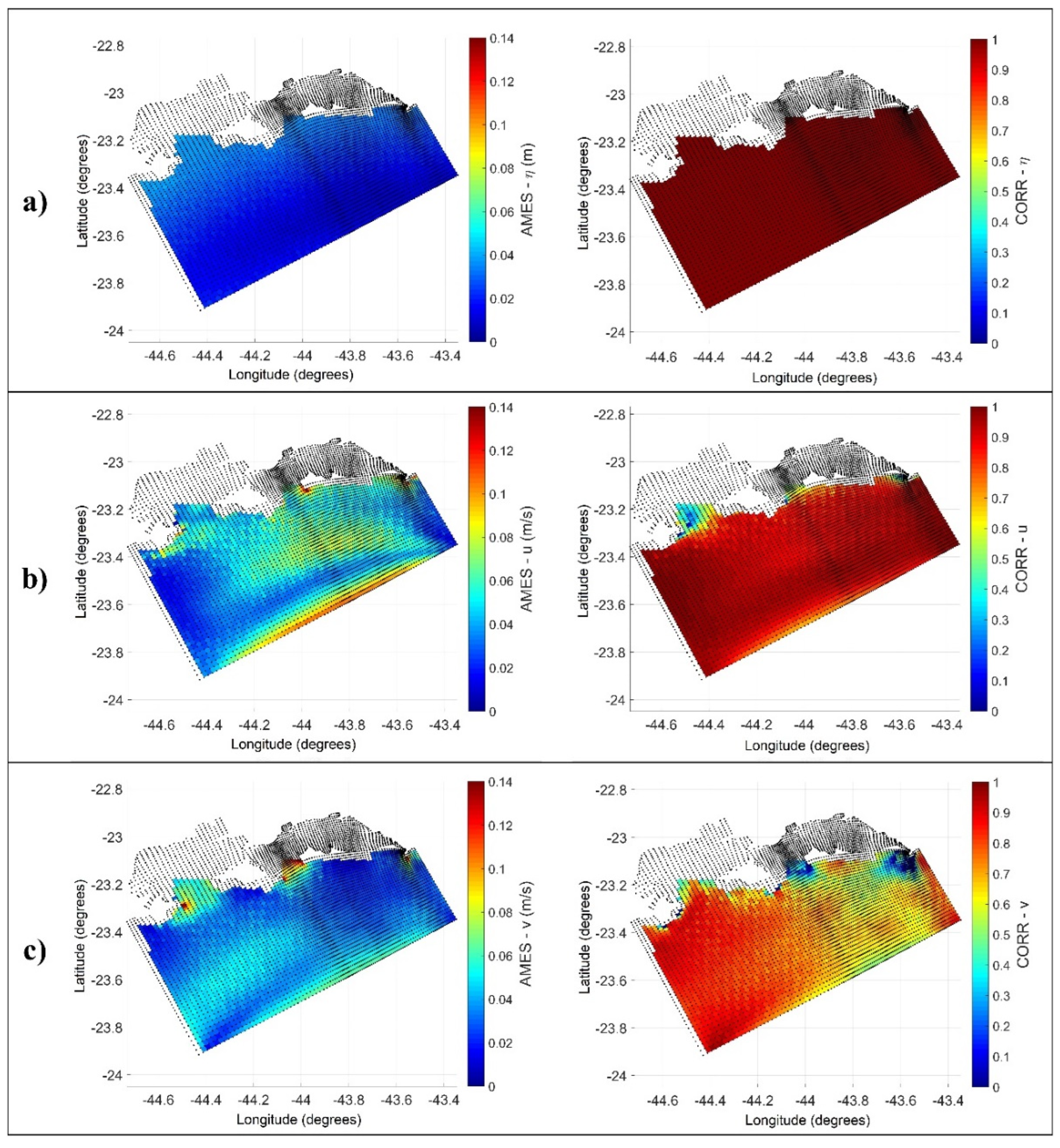
In Figure 3 a comprehensive overview of the comparison results between the coastal model (Delft3D) and the ocean model (HYCOM) for sea water levels and currents is provided. We conducted a spatial analysis of key metrics, including the linear correlation coefficient (CORR) and the absolute mean error statistic (AMES), for the modeling year 2009.

There is a strong agreement regarding water levels, as expected, with an AMES below 0.05 and a CORR exceeding 0.98 throughout the entire domain. In the case of currents, we observed more significant disparities at the southern limit, where the flow is parallel to the border, and in the coastal region, close to the mouths of the bays. The latter are due to the ability of the coastal model to simulate flow patterns within bays and their impact on the continental shelf.

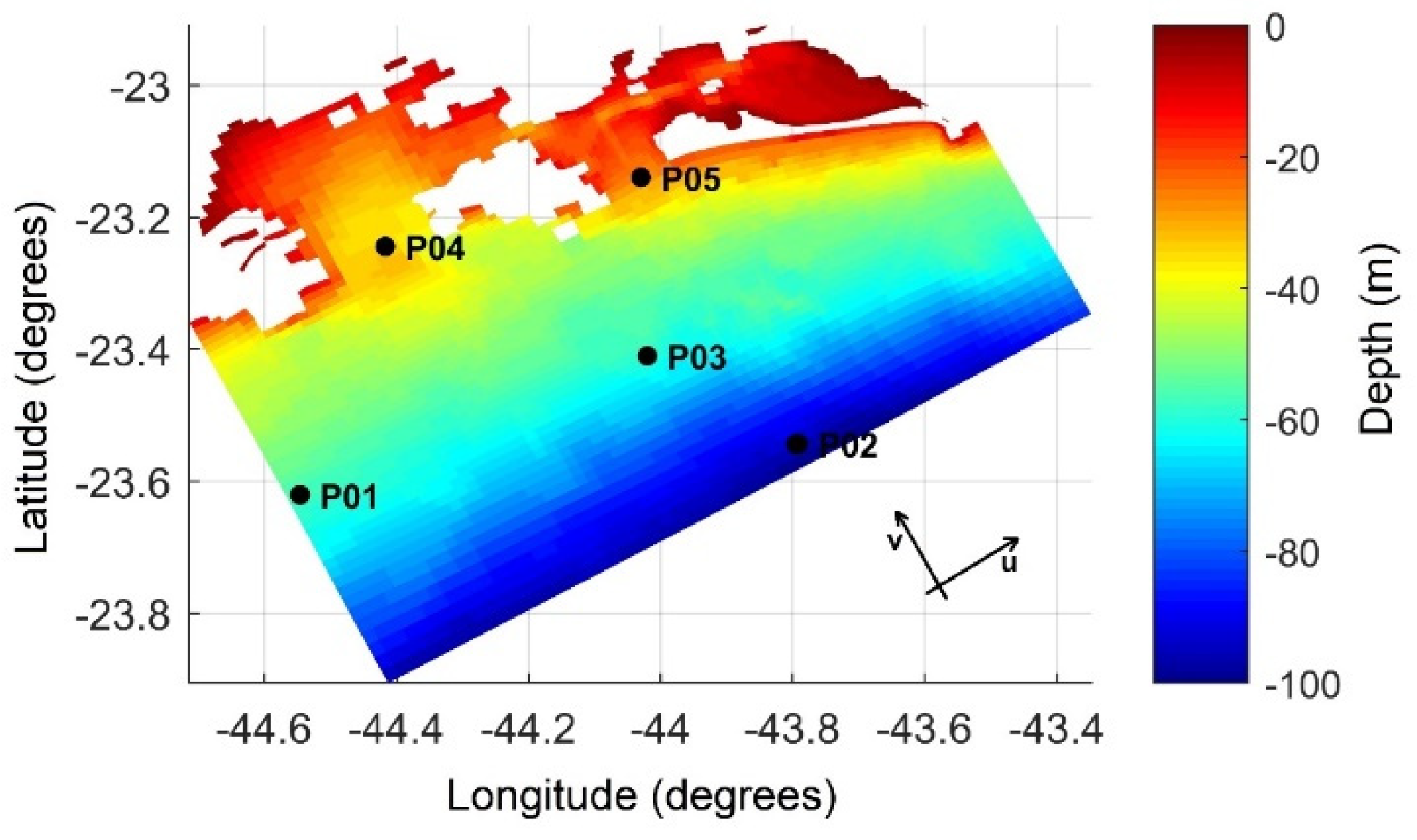
Figure 4 presents the five specific points within the domain where both models are compared. Two points are situated at the boundaries (P01 and P02), one is in the inner part of the domain, and the remaining two are located at the entrances of the bays (transects 04 and 05). The error was calculated for both the total signal and after filtering out the astronomical signal using a 3-day filter.

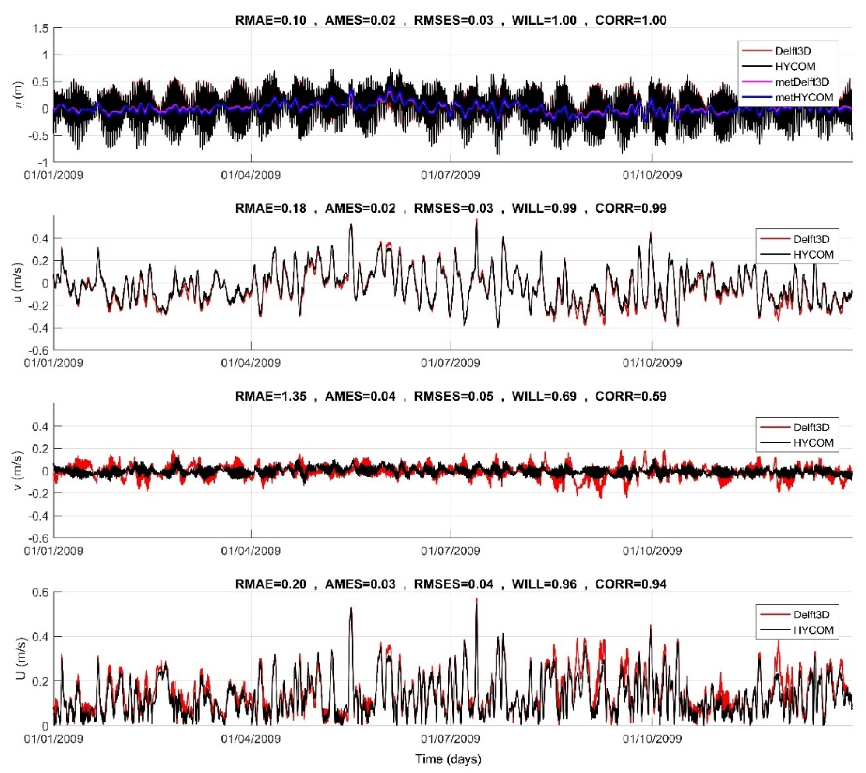
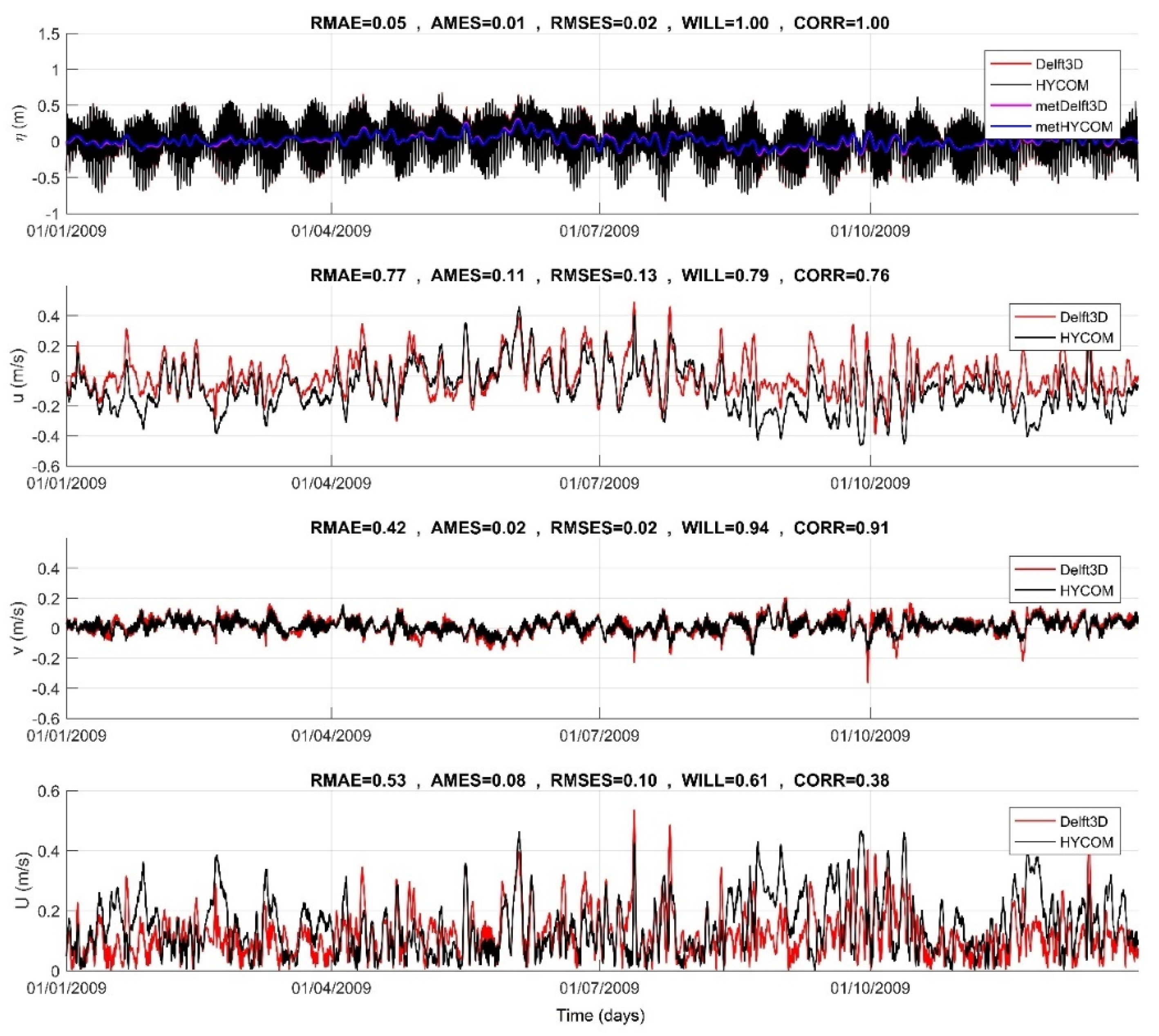
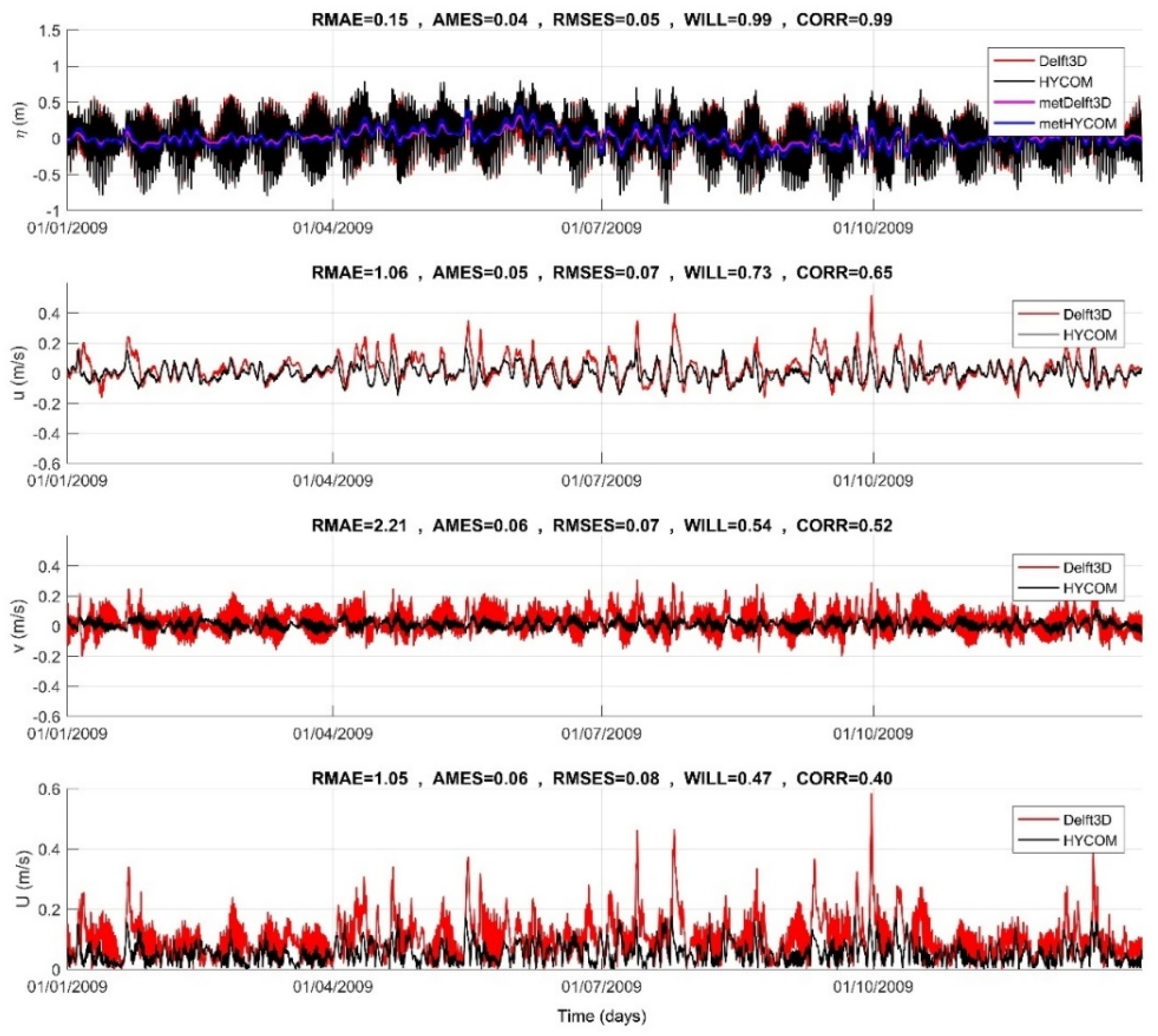
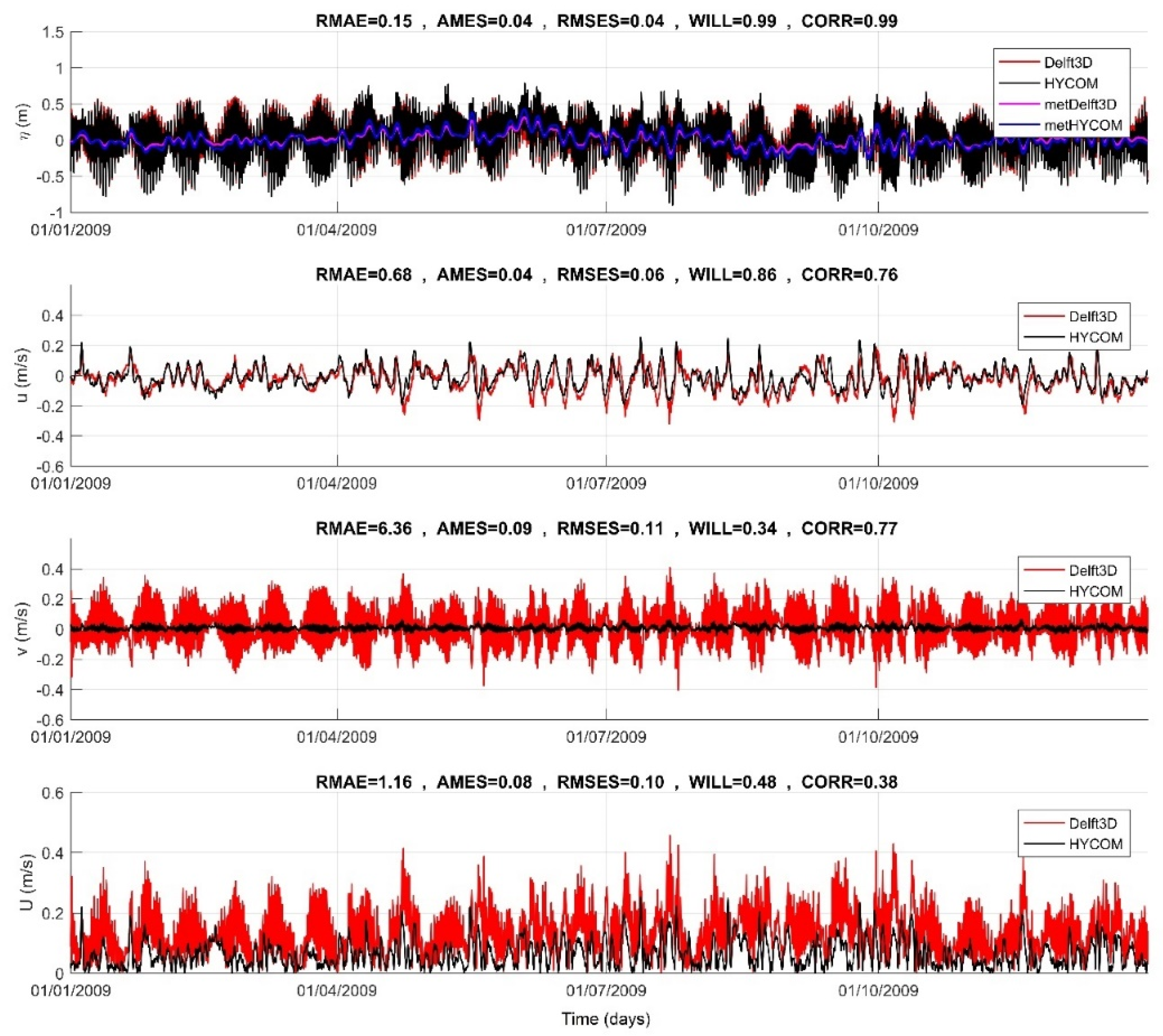
Figure 5, Figure 6, Figure 7 and Figure 8 provide a time series comparison of results between the coastal and ocean models at four distinct points within the domain, as depicted in Figure 4. Point P01 (Figure 5) is situated at the southern lateral open boundary, where the meteorological flow component is predominantly perpendicular to the boundary. Meanwhile, Point P02 (Figure 6) is located at the ocean boundary, where the meteorological flow component primarily aligns parallel to the boundary. The astronomical signal is weaker and acts in the opposite direction to the meteorological signal. As explained in equation 2, the Riemann’s boundary condition exclusively considers the normal velocity component, potentially leading to more effective data transfer between the models at the southern boundary.

At Points P04 (depicted in Figure 7) and P05 (illustrated in Figure 8), situated at the entrances of Ilha Grande Bay and Sepetiba Bay respectively, a pronounced coastal parallel flow induced by meteorological factors is evident. However, it is noteworthy that the current component (v) entering the bays exhibits a notably strong astronomical influence in the currents modeled within the coastal framework, surpassing that observed in the ocean model. This disparity can be attributed to the poor of inner bay representations in the ocean model, as visually indicated by the grid overlap shown in Figure 1. It is worth noting that when a more extensive portion of the bay, particularly Ilha Grande Bay, is encompassed within the ocean model grid, the resulting tidal currents also exhibit increased magnitudes.

The flow component that runs perpendicular to the boundaries, such as the u component at point P01 and the v component at point P02, exhibits relatively low error values when compared to the parallel flow component. As previously mentioned, Riemann's boundary condition fails to capture information about flow parallel to the boundary. At P01, the meteorological signal, which is predominantly found in the u component, is represented with minimal relative or absolute errors. However, it's important to note the suboptimal representation of the astronomical flow signal at this boundary, which is primarily present in the v component.

In contrast, at P02, where the astronomical flow component is mostly perpendicular to the boundary (v component), it is well represented in the nesting. The meteorological flow, which is parallel to this boundary, is also better represented than its counterpart at P01, driven by tidal forces.

Moving to Points P04 and P05 located at the bay entrances, larger errors are observed in the v component due to the ocean model's limitations in accurately representing tidal flows. In Sepetiba Bay, where tidal flow is particularly strong due to its propagation in the elongated bay, more significant differences are noticeable.

It is of paramount importance to underscore the significant differences in the computational grids used in the two models, particularly in the coastal region. The HYCOM model simulations used in this work, which provide boundary conditions for the coastal model (Delft3D), fall short of capturing the intricate geographical features of Ilha Grande and Sepetiba bays, as well as the connection between Sepetiba Bay and the sea via the eastern channel known as "Bacalhau" (as depicted in Figure 1). This lack of detailed geometry significantly hinders the accurate simulation of the robust flood and ebb currents that are characteristic of this area. Moreover, the transmission of tidal signals in water levels from the ocean model to the open boundary of the coastal model enables their propagation into the interior of the bays and connections, a dynamic not replicated in the larger-scale model.

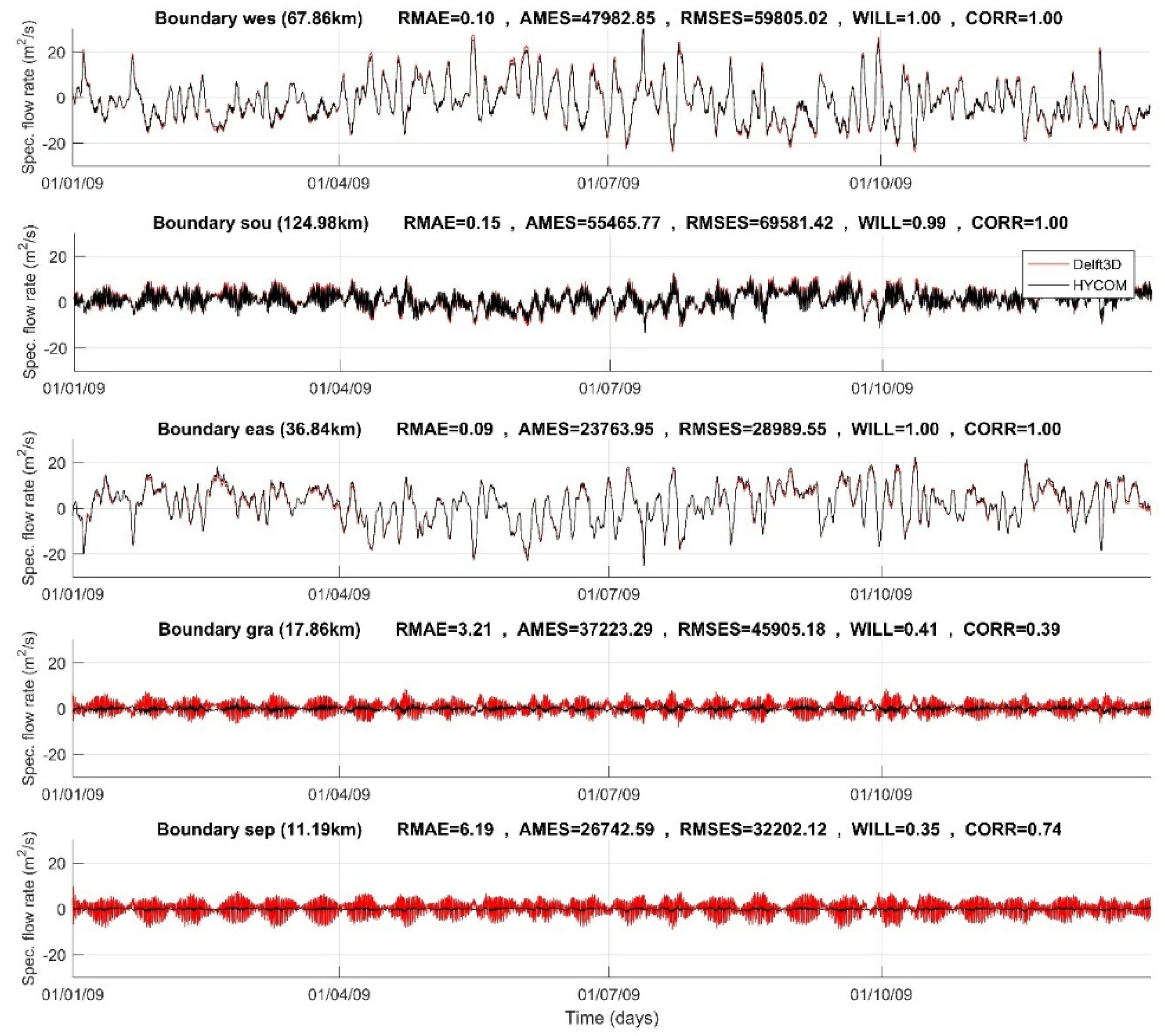
An alternative method for measuring the nesting effects involves examining the flow rates along the boundaries. Positive flow rates indicate an outward direction from the control volume. At both the western (where P01 is situated) and eastern boundaries, meteorological forcing predominantly influences the flow rates, with specific flow rates being comparable, as revealed in Figure 9. Along the southern boundary (where P02 is located), the flow rate is significantly shaped by the onshore-offshore tidal flow, with specific flow rates approximately half the intensity observed along the western and eastern boundaries. As anticipated, at Points P04 and P05, situated at the entrances of the bays (gra and sep), flow rates are also substantially dictated by the tidal dynamics, with a slightly greater impact of meteorological forcing observed in Ilha Grande Bay (gra).

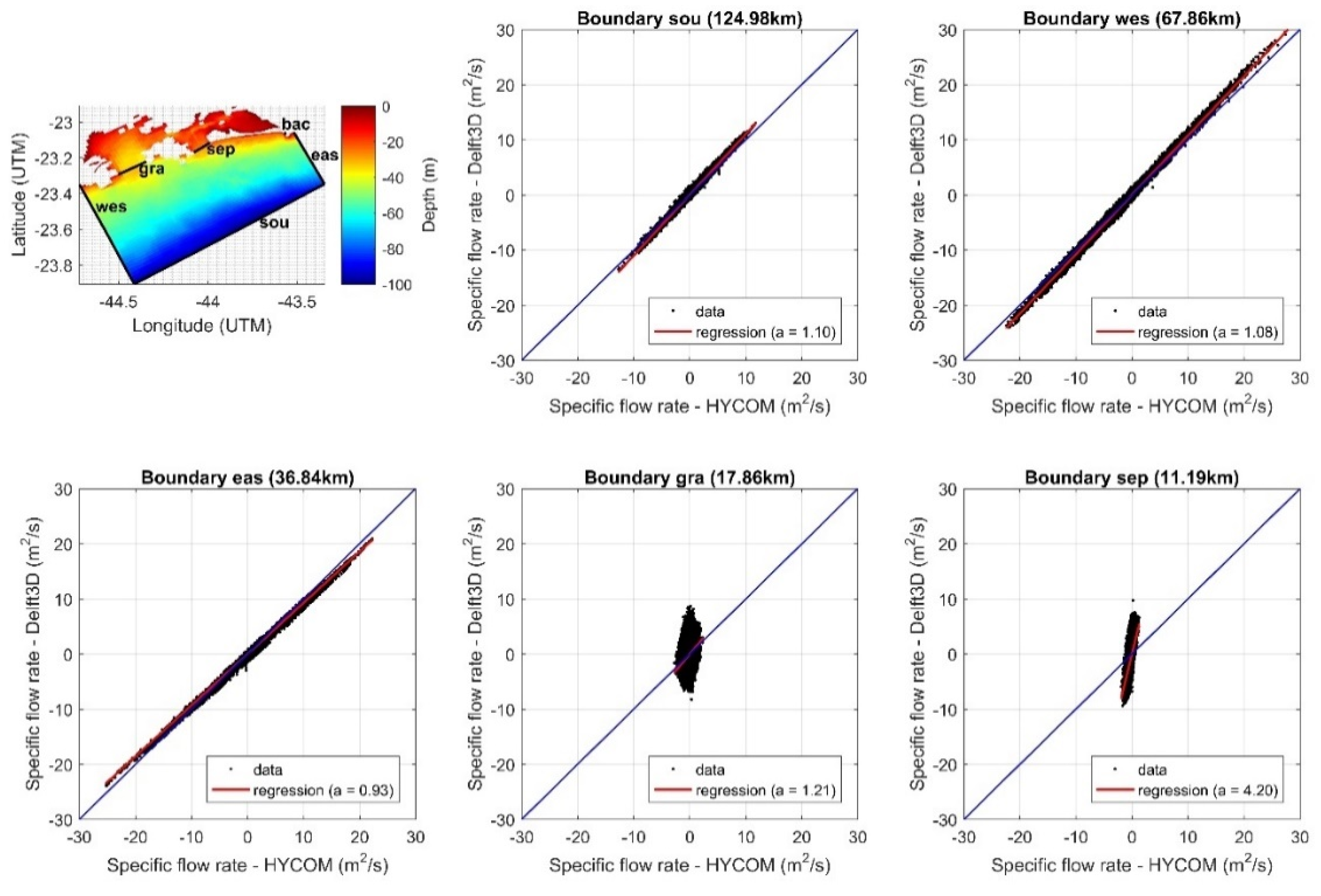
In Figure 10, a linear regression analysis is presented, comparing the time series data from the coastal model (Delft3D) and the ocean model (HYCOM). Along the western (wes), southern (sou), and eastern (eas) ocean boundaries, the angular coefficients are 1.08, 1.10, and 0.93, respectively. These coefficients suggest a slight overestimation by the coastal model of flow along the western and southern boundaries and an underestimation along the eastern boundary. However, at the entrances to the bays, particularly Ilha Grande (gra) and Sepetiba (sep) bays, the angular coefficients are notably larger, measuring 1.21 and 4.2, respectively. As previously discussed, tidal influence dominates the flow patterns at these locations. Consequently, in coastal model, a more accurate description of coastal geometry and bathymetry and the inclusion of bays results in an enhancement in the tidal prism representation.

Table 1 and Table 2, provide insights into the volumes of water crossing the boundaries over the simulation year. Both models exhibit a minor loss of mass, amounting to 0.07% for the ocean model and 0.08% for the coastal model. However, significant disparities emerge when comparing the volume of water crossing these boundaries between the two models. The differences between the models in terms of the volume traversing the boundaries vary considerably, with a 2% variation observed at the western boundary, a substantial 20% and 21% contrast at the southern and eastern boundaries, respectively, and discrepancies of 391% and 219% at the mouth of bays.

3.2. Comparison of Water Level Signal with Available Data

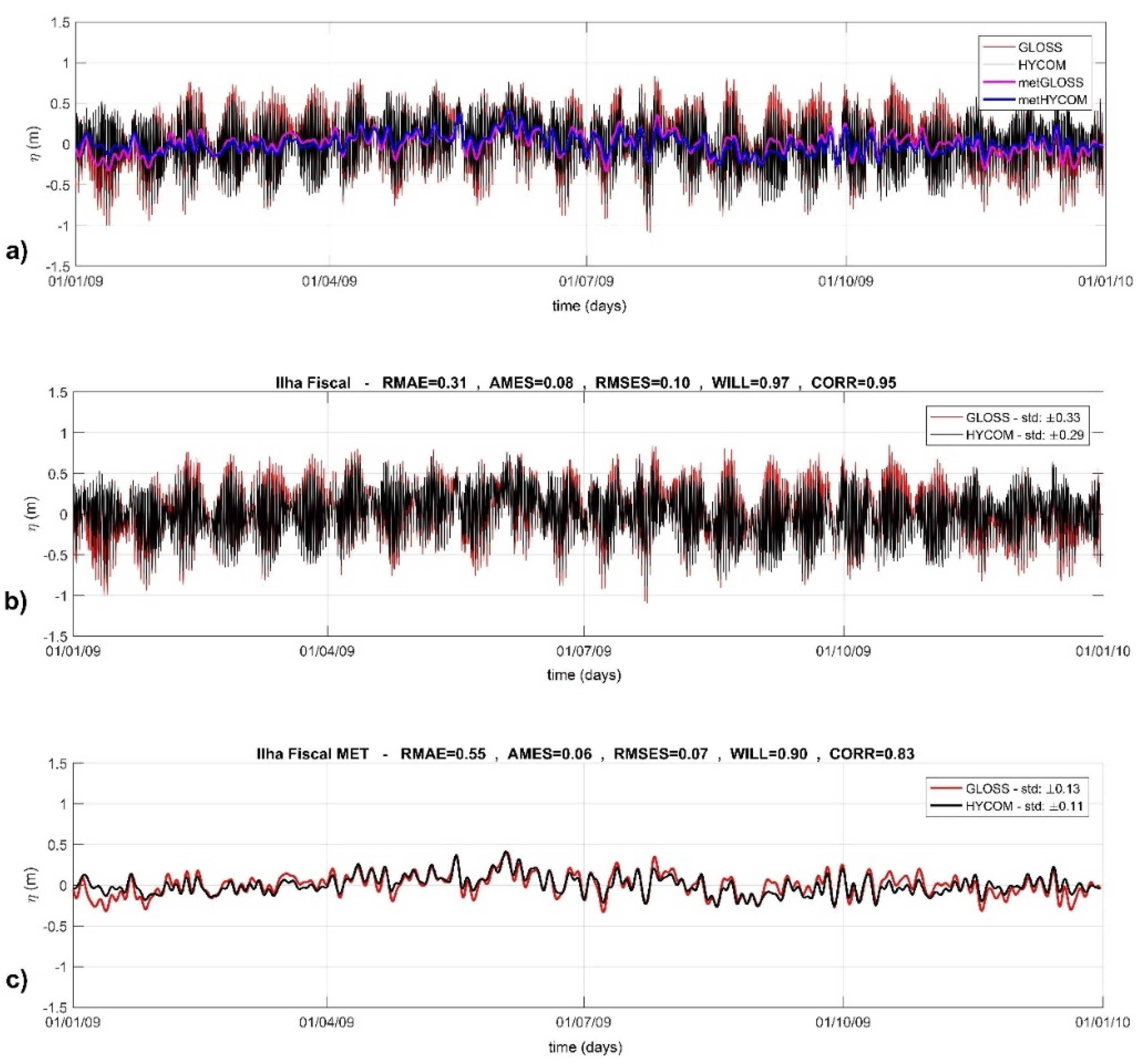
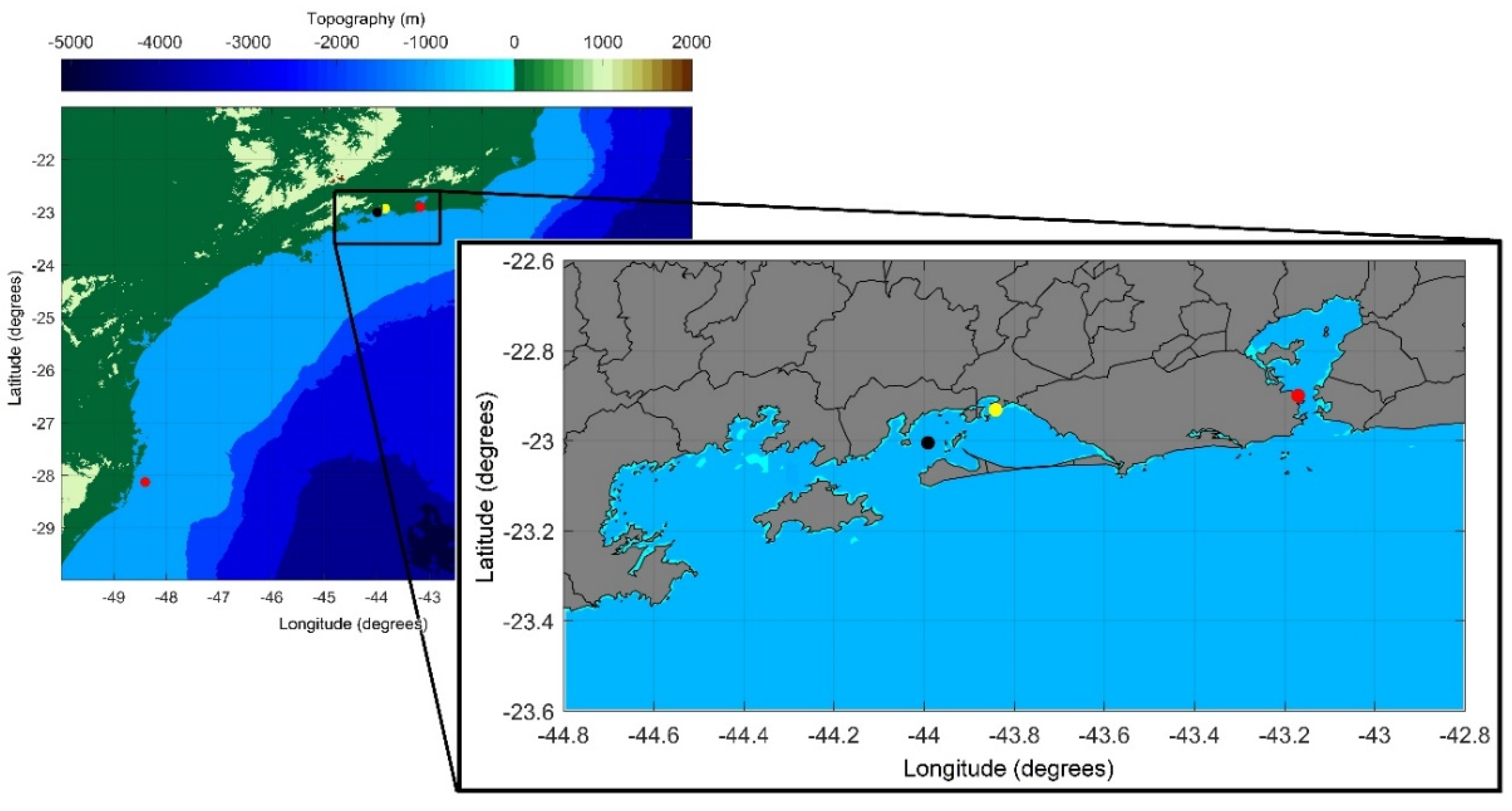
To validate the outcomes of the ocean model, HYCOM, a comparison of sea level time series was conducted, encompassing the entire dataset, considering astronomical and non-astronomical signals. It was compared Fiscal Island gauge station data (as shown in Figure 11) with model results collected at the entrance of Guanabara Bay (as illustrated in Figure 1). An examination of the results reveals an underestimation of the sea level amplitude by the model, a trend that is notably less pronounced during the winter period. This underestimation is substantiated by both absolute and relative error metrics. Nonetheless, the high values of the correlation coefficient and Willmot parameter for both astronomical and non-astronomical signals signal a robust agreement between the model and the observed data, despite the observed underestimation of sea level amplitude.

Southeastern Brazilian Continental Shelf exhibits a highly barotropic response to low-frequency wind forcing, as demonstrated by Stech and Lorenzzetti [63]. Previous studies by Zamudio et al. [64] and Gabioux et al. [44] have highlighted some underestimation in sea level's amplitude when simulating coastal trapped waves using HYCOM, with differences in sea level of approximately 0.15 meters.

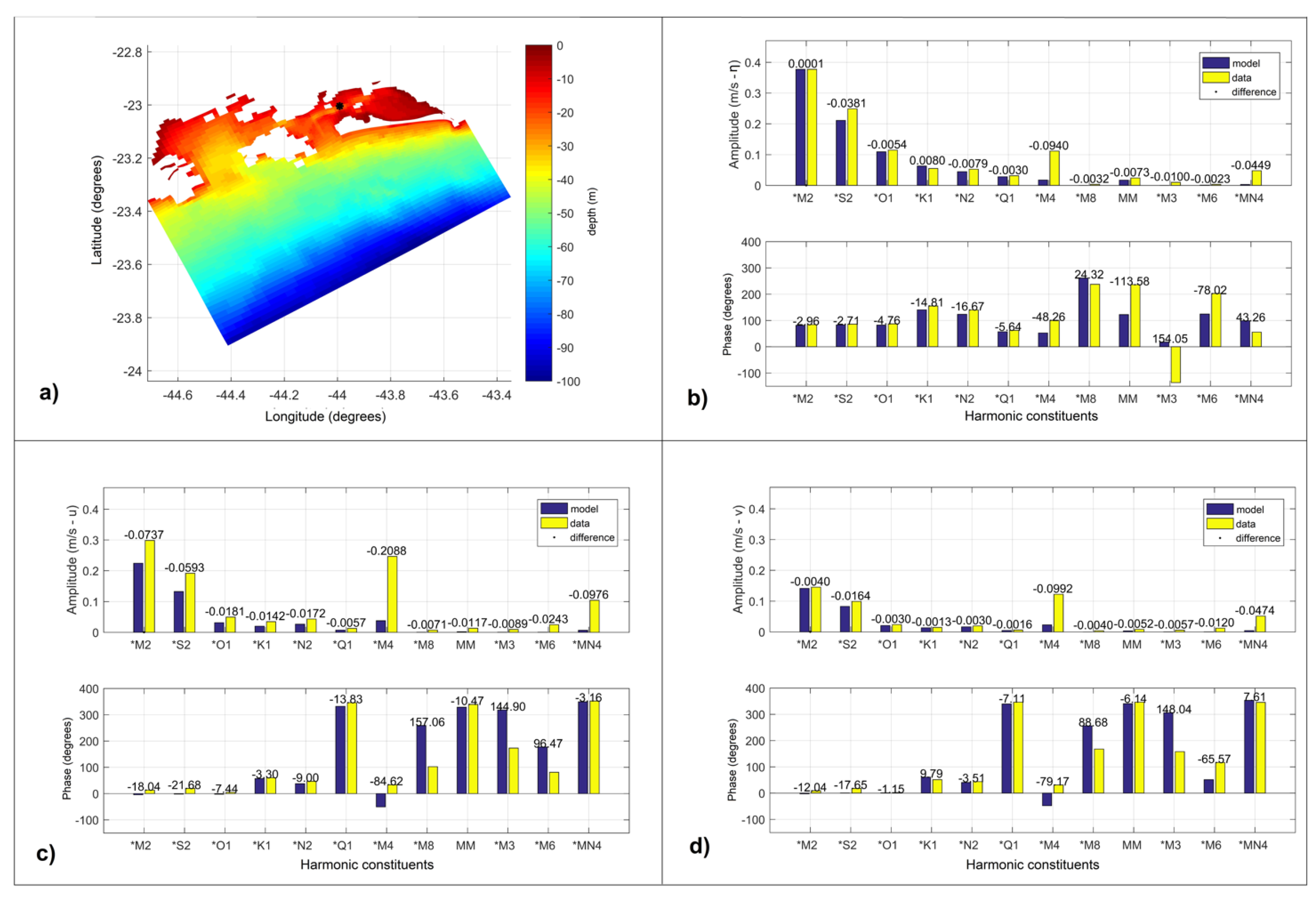
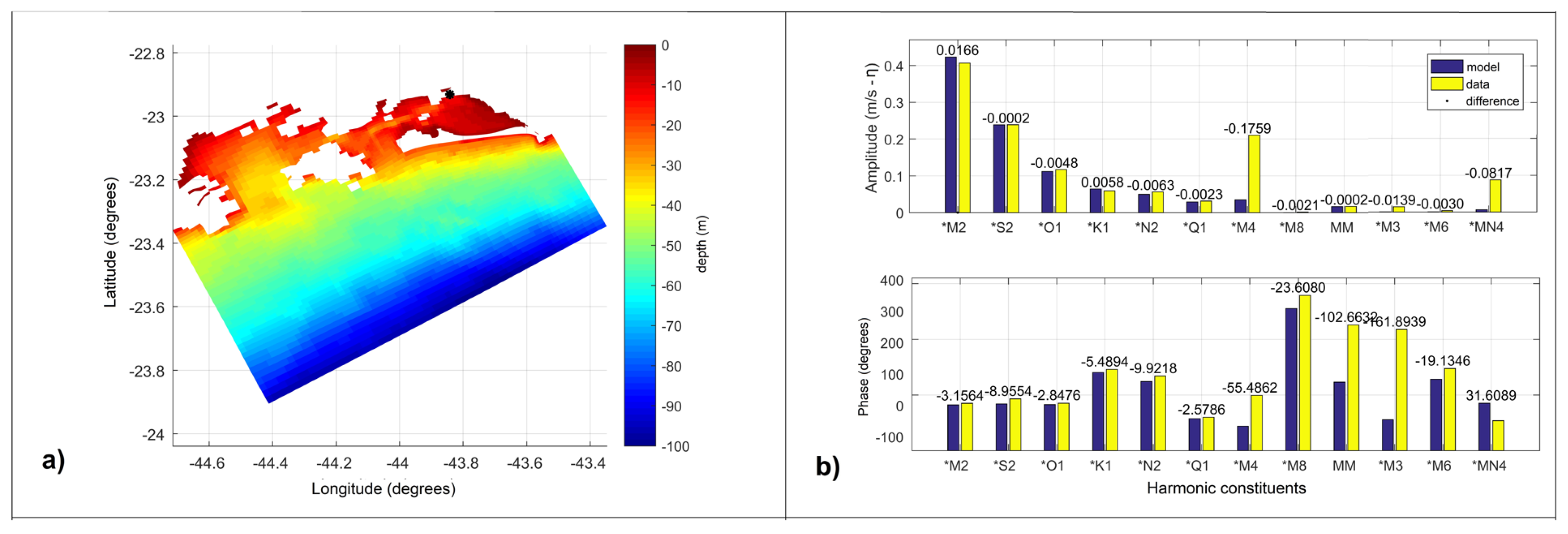
The performance of the coastal model was assessed with a focus on tidal forcing. The astronomical components of the model results were compared to corresponding astronomical components obtained from the data set at Ilha Guaíba station for both water levels and currents (Figure 12), as well as at the Port of Itaguaí station, exclusively for water levels (Figure 13). The model demonstrates a good representation of the diurnal and semidiurnal sea level tidal constituents.

It is worth noting that Teixeira et al. [65] previously observed similar discrepancies when comparing astronomical component data across time series of varying lengths, encompassing different periods of the year. According to these authors, this discrepancy tends to exponentially decrease as the length of the time series used for comparison increases. In the context of currents, the coastal model tends to exhibit larger differences, often resulting in underestimation of amplitudes. Additionally, the shallow water tidal constituents generally display underestimated amplitude values, an outcome that can be expected given that HYCOM incorporates only the eight primary harmonic components [28]. To illustrate, Pairaud et al. [66] highlighted the necessity of prescribing deep ocean boundary conditions for the M4 tidal constituent in ocean models.

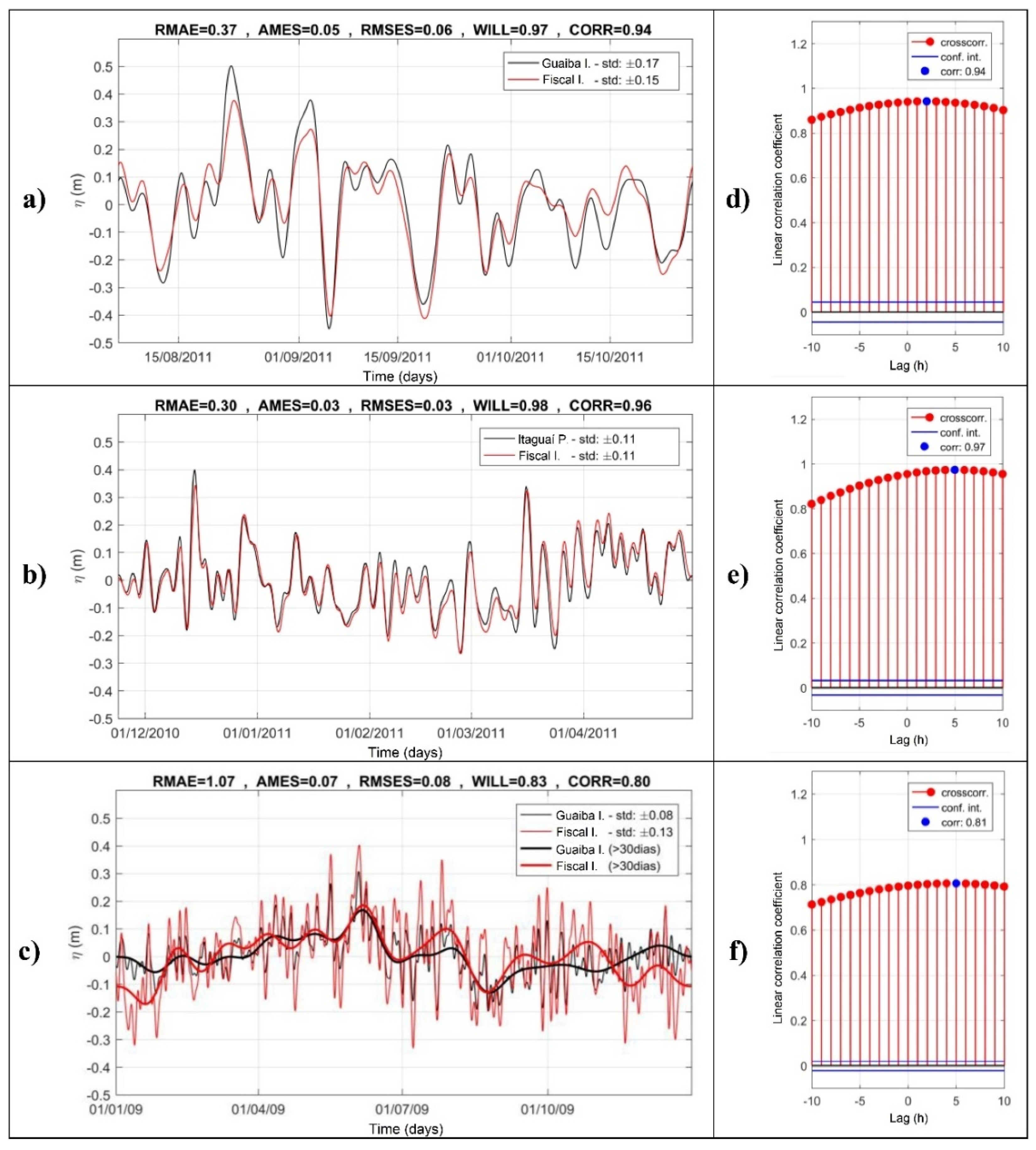
In the first two panels of Figure 14, we compare sea level measurements from the Guaíba Island station (a) and the Itaguaí Port station (b), both situated in Sepetiba Bay, with sea level measurements from the Fiscal Island gauge station in Guanabara Bay. This comparison is made after the removal of astronomical components. As previously discussed, a coastal trapped wave, induced by remote meteorological forces, travels from the southern to the northern Brazilian Continental Shelf. This wave's propagation velocity changes in accordance with the region's geometry, gradually diminishing in amplitude from south to north. The time taken for the coastal trapped wave to propagate from Sepetiba to Guanabara Bay (as shown in Figure 2) was derived from available data and numerical simulations.

Figure 14a,b depict time series and correlation coefficients, while Figure 14d,e showcase the respective time lags between these series. For the Guaíba Island station, the time lag is approximately 2 hours, whereas for the Guaíba Itaguai Port station, it extends to 5 hours. This is coupled with a higher correlation, indicating that the coastal trapped wave is moving northward in both cases.

Moving to the third panel of Figure 14c, we compare modeling results to measurements after the removal of astronomical components for the entire simulated year of 2009. The data is collected from the Fiscal Island gauge station in Guanabara Bay and the modeling results for Sepetiba Bay at the Guaíba station. As expected, correlations among the series are notably lower, but the primary characteristics are well represented. In the context of the meteorological signal's seasonality, a 30-day low-pass filter is also presented in Figure 14c. The numerical simulations closely follow the annual pattern observed by Campos et al. [67], who analyzed observations from the Port of Santos in São Paulo, revealing a higher number of positive extremes (40.2%) in autumn and a greater number of negative extremes (47.2%) in spring. A similar pattern is observed by Kjerfve et al. [34] in their observations from the Ilha Grande Channel.

Table 3 presents cross-correlation and time lag values across various time periods. For long time series, it tends to stabilize around a 5-hour time lag. The propagation speed averages approximately 5 m/s. Notably, this value is significantly lower than the coastal wave propagation speed of 12.2 m/s observed from Imbituba to Sepetiba Bay (as illustrated in Figure 2), which is situated 748 km south and exhibits a time lag of 17 hours with a cross-correlation of 0.83. These findings are consistent with previous research conducted by Castro and Lee [27], França [28] and Dottori and Castro [29].

As suggested by Melo Filho [16], the reduction in propagation speed can be attributed to the narrowing of the Brazilian Continental Shelf, a notion similarly emphasized by Brink [23] and Platov [10]. In the southern region, between Imbituba and Sepetiba Bay, the Continental Shelf width, extending from the coast to the 200m isobath, spans approximately 200 km. However, between Sepetiba Bay and Ilha Fiscal, this width is approximately halved, measuring roughly 100 km. This phenomenon is a result of energy dissipation due to bottom friction, as noted by Gutiérrez et al. [68], and the significant dispersion of energy between wave propagation modes in stratified ocean conditions, as highlighted by Wilkin and Chapman [69].

The standard deviation of sea level varies between ±0.11m and ±0.17m, with lower values recorded during the autumn season (as shown in Figure 6a,b) in Sepetiba Bay. Similarly, measurements in Guanabara Bay for the year 2009 exhibit a comparable standard deviation of ±0.13m (as depicted in Figure 3). Notably, the numerical results from the ocean model (HYCOM) show a slightly lower sea level standard deviation of ±0.11m, indicating an underestimation of the meteorological signal. This observation aligns with findings reported by França [28], Carvalho [55] and Daher et al. [70].

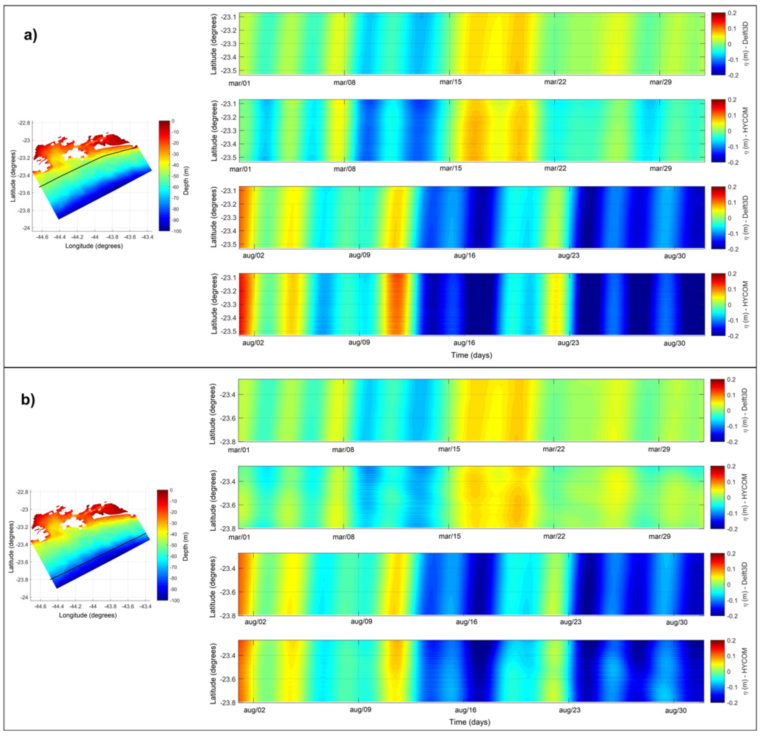
Figure 15 provides a comparative analysis of the temporal variability in sea level, with the astronomical signal removed, using a 3-day filter for water level data for the year 2009. This comparison is made between the ocean model (HYCOM) and the coastal model (Delft3D). Two coastal transects are illustrated: one situated closer to the coastline at a depth of approximately 50 meters (a), and another farther offshore at approximately 80 meters in depth (b). The results are presented for two scenarios: the first represents a less intense meteorological signal observed in March (upper panels), and the second depicts a stronger meteorological signal observed in August (lower panels). The temporal evolution along the transect, indicated by latitude, showcases the propagation of the meteorological wave towards the north.

At a central point along the transect, both models exhibit a similar standard deviation of ±0.08 meters near the boundary. However, when we examine a point closer to the bay's entrance, nearer to the coastline, we observe that the standard deviation of sea level is ±0.08 meters for Delft3D and ±0.11 meters for HYCOM. This discrepancy indicates a subtle attenuation of the meteorological signal near the coast after employing the coastal model nesting, resulting in a loss of signal amplitude in comparison to the ocean model.

3.3. Spatial Analysis of Tidal and Non-Tidal Signals

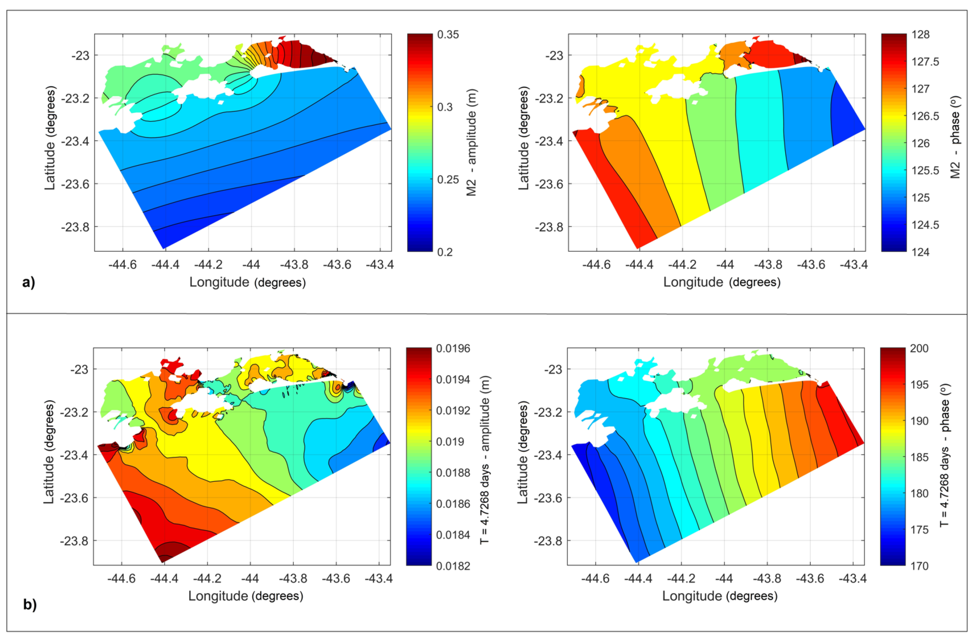
To gain a deeper understanding of the patterns associated with tidal and non-tidal signals driven by meteorological forces, we first examined the results from the simulation of coupled models, encompassing both S1 and S2 scenarios. We focused on the spatial distribution of the amplitude and phase of the astronomical constituent M2, with reference to the simulation that considers the cumulative outcome of the HYCOM model (as depicted in Figure 16a).

Our observations revealed a southward phase propagation, consistent with the findings of Harari and Camargo [38] for the majority of the primary tidal constituents. Notably, the phase difference between the two ends of the boundary parallel to the coastline is relatively small, measuring nearly 4 degrees. As we approach the entrances of the bays, this phase aligns itself parallel to these entrances, progressing further inland in phase at the two main entry points and amplifying its effect as it moves deeper into Sepetiba Bay. This phase propagation aligns with Signorini's [33] observations of tidal signals propagating in phase within the estuarine system's primary entrances.

The amplitude isolines exhibit a nearly perpendicular orientation to the coast, indicating similar amplitudes at the primary system entry points and amplification as they progress further inland within the system.

Regarding the constituent with a period of 4.73 days, representing the meteorological signal (as illustrated in Figure 16b), our observations revealed a phase propagation toward the northeast, consistent with the findings of Castro and Lee [27]. A significant phase difference exists between the two ends of the boundary parallel to the coast, amounting to nearly 30 degrees. This phase difference is less pronounced within Sepetiba Bay but becomes more prominent in the channel between Ilha Grande and the mainland. The amplitude of this signal demonstrates a correlation with the phase, with greater amplitudes observed in Ilha Grande Bay, accompanied by a more pronounced level gradient in the channel between the bays. It's worth noting that the amplitudes of this signal are notably smaller when compared to M2.

In the spatial distribution of our simulation results (depicted in Figure 17), it's evident that during the flooding tide, water accumulates inside the bays, particularly within Sepetiba Bay. The current patterns align with the water level, flowing in the direction of the water accumulation and intensifying around the bottleneck regions in the bathymetry. This pattern remains consistent during the ebb tide but in the opposite direction.

The spatial distribution of the simulation, focusing solely on astronomical effects (S2 scenario), exhibits a similarity in the flood and ebb patterns within the interior of Sepetiba Bay. However, in Ilha Grande Bay and the surrounding marine areas, these patterns differ significantly, both in terms of intensity and direction. Predominantly, the currents flow to the southwest, aligning with the passage of the meteorological signal.

This spatial pattern aligns with prior research findings [35,36,71]. It is evident that flood currents within Sepetiba Bay are more intense than ebb currents, a phenomenon also observed in Ilha Grande Bay, as highlighted by Fragoso [35] and Cavalcante [36]. This pattern underscores the significant influence of tides on circulation in Sepetiba Bay compared to Ilha Grande Bay, an observation in line with Signorini's [32] research.

The spatial disparities in the time series of results between the two simulations become more apparent in the spatial distribution of the differences between them (as depicted in Figure 18). Notably, all values are negative across the entire domain, signifying that the scenario neglecting the meteorological tide underestimates sea levels in a spatially varied manner. The difference in sea level is relatively low, approximately 10-3 meters, with more pronounced effects in the open sea and the channel connecting the two bays. The inner section of Sepetiba Bay records lower values, an area where the astronomical signal dominates.

Examining Ilha Grande Bay, its westernmost region exhibits differences close to zero, while certain areas display positive values, indicating a greater intensity of currents in the simulation without the meteorological effect, resulting in speed increases of approximately 0.01 m/s. Closer to the bay's entrance, negative differences are observed, implying a higher intensity of currents in the simulation incorporating the meteorological effect, leading to reductions in current intensity of up to 0.15 m/s.

Concerning Sepetiba Bay, most of the area exhibits differences with values close to zero. However, specific regions stand out, particularly at the bay's entrance, where the simulation with the meteorological effect portrays the highest current intensities. In contrast, the modeling without the meteorological effect underestimates current intensities by approximately 0.07 m/s in this region.

In a study by Signorini [33], simulations were conducted to investigate the effects of phase lag on open boundaries for tidal signals (M2, S2, and M4). It was observed that no phase lag resulted in very low currents in Ilha Grande Channel (approximately 0.04 to 0.05 m/s). However, the introduction of a phase lag (20 minutes) led to an intensification of currents in Ilha Grande Channel, reaching around 0.20 m/s, with alternating flow directions. Nevertheless, this scenario did not align with the in situ data analyzed by the author. Nonetheless, this experiment emphasized that the presence of a lag in open boundary sea levels could be a crucial factor in understanding the intensification of currents in Ilha Grande Channel, owing to the generation of a barotropic pressure gradient resulting from sea level disparities.

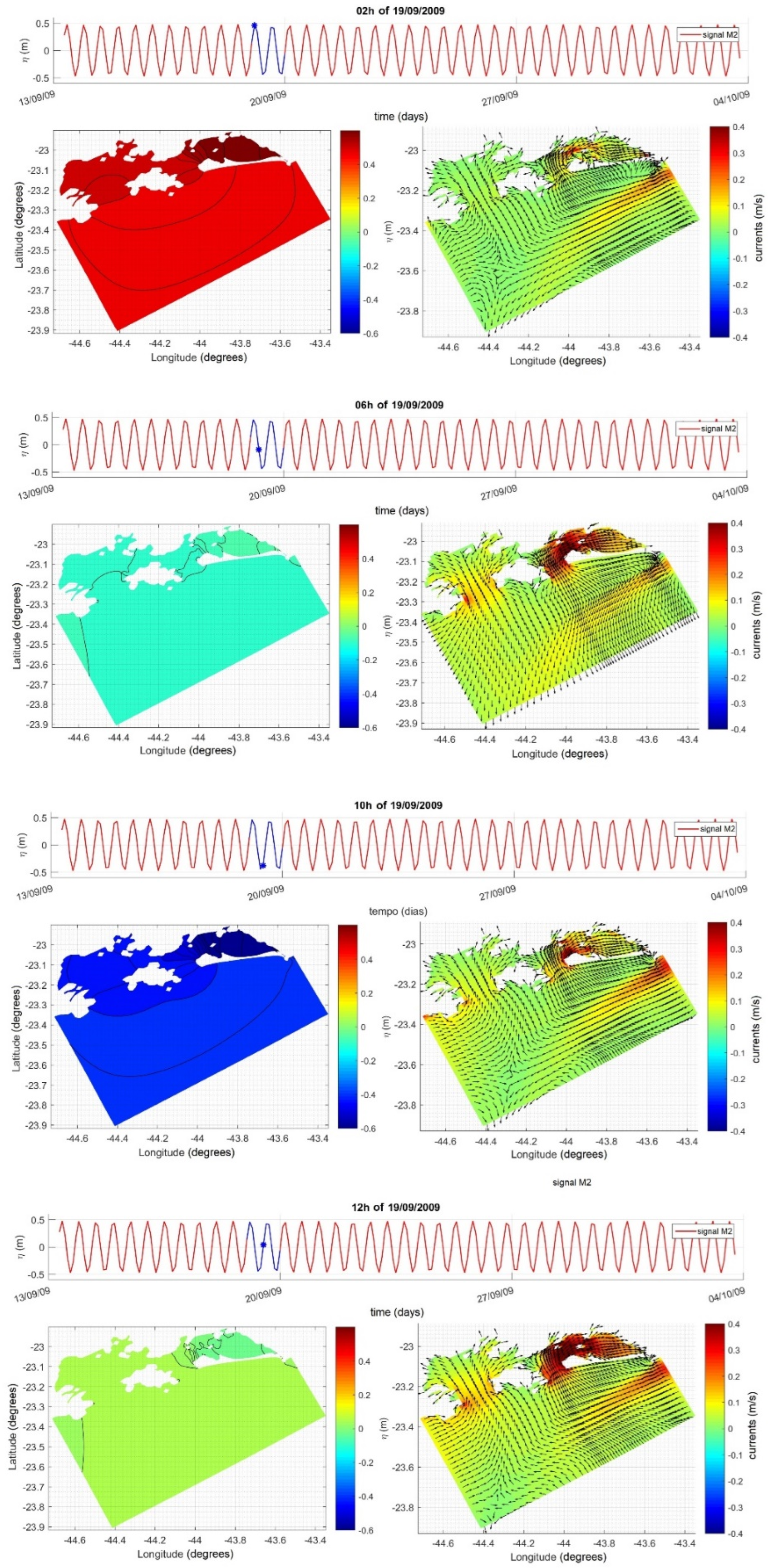
To gain a deeper understanding of the distinct behavior of astronomical and meteorological signals in our study area, we conducted an examination of the propagation of only the M2 component within the study area. This signal was introduced solely at the sea level, and we anticipated a response in the currents. We tested variations in the propagation direction and amplitude of this signal but found no significant alterations in the general patterns of level and current distribution. The relatively small difference in sea level between the eastern and western boundaries contributes to the more stationary nature of the astronomical signal. 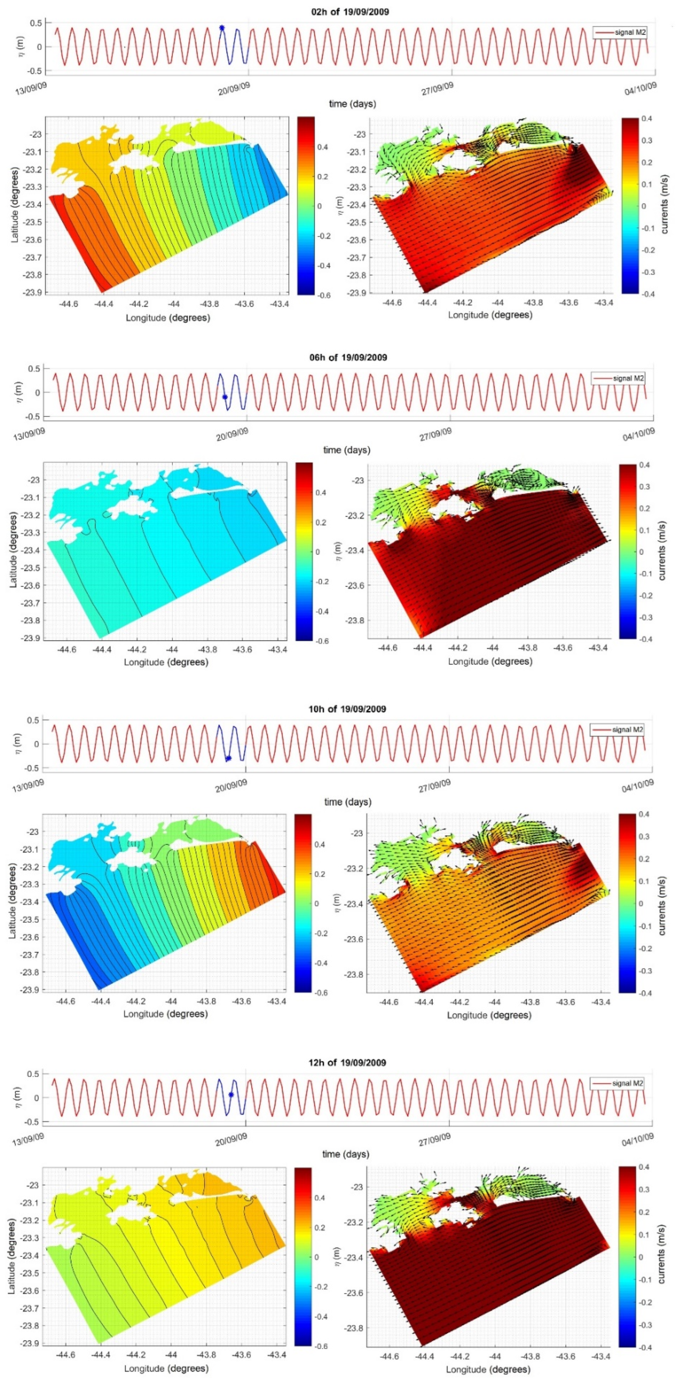To further explore this, we conducted experiments introducing a lag of 1 minute (S3 scenario), akin to the observed environmental conditions (as seen in Figure 19), and a lag of 4.92 hours (S4 scenario), mirroring the meteorological signal (as seen in Figure 20).

While the M2 tidal lag of just 1 minute exhibited behavior closely reflecting the overall astronomical signal, the 4.92-hour lag demonstrated characteristics remarkably akin to those of the meteorological signal. Only minor alterations in current patterns were observed, which can be attributed to the introduction of boundary levels. Notably, the M2 currents associated with the 4.92-hour lag were more robust than the original meteorological signal, likely due to the greater amplitude imposed on this signal. Directional changes were also evident, as M2 propagated southward, contrary to the meteorological signal, as discussed by (Harari and Camargo [38]).

From these experiments, we can infer that the stationary behavior of the astronomical signal is a direct consequence of its minimal lag at the external boundary. This short lag results in a small level gradient between the lateral boundaries compared to the gradient between the boundary parallel to the coast and the coastline. Consequently, at the bay entrances, the flow perpendicular to the coast results in the characteristic flood and ebb flows. As the signal enters Sepetiba Bay, due to the level gradient between the entrance and the innermost portion of the bay, at Bacalhau channel, the wave signal goes to transition into a progressive state with expressive tidal currents in this bay.

Increasing the lag of the wave signal leads to a greater level gradient between the lateral boundaries, favoring flow parallel to the coast, as observed in the meteorological signal. While this flow exhibits higher intensity outside the bays, a portion of it finds its way into the bay entrances, bypassing Ilha Grande and passing through the channel between the island and the mainland, which intensifies currents in this region.

4. Conclusions

The water level observations from our model, incorporating both astronomical and meteorological signals, at a point within Sepetiba Bay, exhibited a standard deviation of ± 0.32m. However, upon removal of the astronomical signal, the same data still showed a standard deviation of ± 0.08m. This indicates that in Sepetiba Bay, while more affected by tides within the entire system, meteorological signal still accounts for 25% of the total variance. Thus, it becomes evident that the meteorological forcing cannot be disregarded in this system.

Comparing the meteorological forcing represented by the ocean model to available data reveals that the main features align well with the observed conditions in the area. Notably, the propagation speed exhibits northward movement in phase with the sea level, characteristic of Coastal Trapped Waves. While this pattern aligns with literature reports, there is an observed underestimation of the signal's intensity, which has also been reported previously. Furthermore, the coastal model highlights a further attenuation of the meteorological signal's intensity near the coastline.

The coupling of the coastal model (Delft3D) with the ocean model (HYCOM) using Riemann's invariants proves effective in driving the coastal model with the meteorological sea level signal. This approach accounts for the velocity component normal to the boundary, and the coastal model aptly captures the flows along both the west and east boundaries, which are perpendicular to the along-shelf flow. The south boundary, parallel to the bathymetry, exhibits more intense tidal flow, yet the coastal model accurately simulates the boundary flows in all cases, particularly when assessing flow rates entering and exiting the boundaries. Thus, the ocean model adeptly captures the meteorological forcing on the continental shelf and transfers it into the coastal domain's interior. This coastal model is tailored to address the intricacies of coastal geometry that are often overlooked in larger-scale models.

Focusing on the patterns of the tidal and non-tidal signals, a notable phase lag is observed in the meteorological signal (assessed over a period of 4.73 days) in the open sea and the channel between Guaíba Island and the mainland. This phase lag is more pronounced in the meteorological component compared to the astronomical component (M2 analysis). The observed gradient of amplitudes and current intensities corresponds with this, with more intense currents seen in the meteorological signal compared to the astronomical one. Conversely, along the interior of Sepetiba Bay larger gradients of amplitude and phase in the astronomical signal are observed.

An examination of simulations with and without the meteorological signal underscores the significance of including the meteorological signal, as it significantly impacts currents. The sea level and current intensities in simulations considering the meteorological signal align well with existing literature, accurately representing ebb and flow patterns. Conversely, excluding this signal results in an underestimation of intensities, particularly in the open sea, the channel between Guaíba Island and the mainland, and a substantial portion of Ilha Grande Bay.

In M2 signal propagation tests, we observed that the signal behaves similarly to the meteorological signal when a comparable lag is applied to the external boundary. The minimal lag of the astronomical signal at the open border results in a minor level gradient between the lateral boundaries, favoring only perpendicular coastal flow (flood and ebb). An increase in the lag leads to a greater level gradient between the lateral boundaries, favoring flow parallel to the coast, a behavior consistent with the meteorological signal.

In conclusion, the distinct hydrodynamic patterns associated with astronomical and meteorological signals are a reflection of their propagation characteristics on the platform. The meteorological signal generates a level gradient parallel to the coast, intensifying currents in that direction. The differential level gradient between the main entrances of the bays results in flow around Ilha Grande, playing a pivotal role in intensifying currents in the channel between the island and the mainland, exacerbated by the channel's narrow geometry. On the other hand, the astronomical signal displays a high-level gradient onshore, driving more robust ebb and flow currents at the bays entrances. The channel between Ilha Grande and the mainland serves as a point of convergence/divergence of this flow, with very low current velocities. Further investigations into baroclinic influences and nonlinear interactions of sea level signals on circulation in the inner portions of the bays are recommended for a further understanding of their roles in the circulation dynamics.

Author Contributions

Conceptualization, N.P. and S.V.; methodology, N.P.; software, N.P.; validation, N.P.; formal analysis, N.P.; investigation, N.P.; resources, N.P. and S.V.; data curation, N.P.; writing—original draft preparation, N.P.; writing—review and editing, N.P., S.V., M.G.1 and M.G.2; visualization, N.P.; supervision, S.V.; project administration, S.V.; funding acquisition, S.V. All authors have read and agreed to the published version of the manuscript.

Funding

First author was financially supported by CAPES (Coordenação de Aperfeiçoamento de Pessoal de Nível Superior – Brazil) – Finance Code 001. Second and third authors were also financially supported by CNPq (Conselho Nacional de Desenvolvimento Científico e Tecnológico) through Grants 310132/2019-3 and 309055/2022-9.

Data Availability Statement

The data used in this work is available on request to the corresponding author.

Acknowledgments

We also acknowledge the support of our colleagues and everyone who contributed to this project.

Conflicts of Interest

The authors declare no conflict of interest.

References

Nicholls, R.J.; Kebede, A.S. Indirect impacts of coastal climate change and sea-level rise: the UK example. Climate Policy 2012, 12, sup01, S28–S52. [CrossRef]
Andrade, M.M.; Toldo, E.E.; Nunes, J.C.R. Tidal and subtidal oscillations in a shallow water system in southern Brazil. Brazilian Journal of Oceanography 2018, 66, 3, 245–254. [CrossRef]
WMO. Atlas of mortality and economic losses from weather, climate, and water extremes (1970–2019). Geneva, Switzerland: World Meteorological Organization (WMO), 2021, pp. 90.
Pugh, D. Tides, surges, and mean sea-level. New York: John Wiley & Sons, 1987, pp. 486.
Bowden, K. F. Physical Oceanography of Coastal Waters. England: Ellis Horwood Limited, 1983, pp.302.
Open University. Waves, tides and shallow-water processes. 2nd. ed.; Oxford: Butterworth-Heinemann, 1999, pp.227.
Marone, E.; Camargo, R. Marés meteorológicas no litoral do estado do Paraná: o evento de 18 de Agosto de 1993. Nerítica 1994, 8, 1–2,73–85.
Wang, B. Kelvin waves. In Encyclopedia of Atmospheric Sciences; M. Shankar, Ed.; Elsevier Science Ltd, 2002, pp. 1062–1068. https://doi.org/10.1006/rwas.2002.0191.
Wang, D. P.; Mooers, C. N. K. Coastal-trapped waves in a continuous stratified ocean. Journal of Physical Oceanography 1976, 6, 853–863. https://doi.org/10.1175/1520-0485(1976)006%3C0853:CTWIAC%3E2.0.CO;2.
Platov, G. A. The influence of shelf zone topography and coastline geometry on coastal trapped waves. Numerical Analysis and Applications 2016, 9, 3, 231–245. [CrossRef]
Mysak, L. A. Topographically trapped waves. Annual Review of Fluid Mechanics 1980, 12, 1, 45–76. [CrossRef]
Idier, D.; Bertin, X.; Thompson, P.; Pickering, M.D. Interactions Between Mean Sea Level, Tide, Surge, Waves and Flooding: Mechanisms and Contributions to Sea Level Variations at the Coast. Surveys in Geophysics 2019, 40, 6, 1603–1630, 2019. [CrossRef]
Wang, D.P.; Elliott, A.J. Non-Tidal Variability in the Chesapeake Bey and Potomac River: Evidence for Non-Local Forcing. Journal of Physical Oceanography 1978, 8, 225–232. [CrossRef]
Garvine, R. W. A simple model of estuarine subtidal fluctuations forced by local and remote wind stress. Journal of Geophysical Research 1985, 90, C6, 11945-11948. [CrossRef]
Zhong, L.; Li, M.; Zhang, D.-L. How do uncertainties in hurricane model forecasts affect storm surge predictions in a semi-enclosed bay? Estuarine, Coastal and Shelf Science 2010, 90, 2, 61–72. [CrossRef]
Melo Filho, E. Maré Meteorológica na Costa Brasileira. Associate Professorship thesis, Universidade Federal de Rio Grande, Rio Grande, Brazil, 2017. Available online: https://www.researchgate.net/profile/Eloi-Melo/publication/318710781_Mare_Meteorologica_na_Costa_Brasileira/links/5979090f0f7e9b27772a250a/Mare-Meteorologica-na-Costa-Brasileira.pdf (accessed on 20 November 2023).
Truccolo, E.C.; Franco, D.; Schettini, C.A.F. The low frequency sea level oscillations in the northern coast of Santa Catarina, Brazil. Journal of Coastal Research 2006, SI 39, 547–552.
Oliveira, M.M.F.; Ebecken, N.F.F.; Santos, I. A.; Neves, C. F.; Caloba, L. P.; Oliveira, J. L. F. M. Modelagem da maré meteorológica utilizando redes neurais artificiais: uma aplicação para a Baía de Paranaguá – PR, Parte 1: Dados meteorológicos da estação de superfície. Revista Brasileira de Meteorologia 2006, 21, 2, 220–231.
Verlaan, M.; Zijderveld A.; de Vries, H.; Kroos, J. Operational storm surge forecasting in the Netherlands: developments in the last decade. Philosophical Transactions of the Royal Society A: Mathematical, Physical and Engineering Sciences 2005, 363, 1831, 1441–1453. [CrossRef]
Cavalcante, S.L.S.; Rosman, P.C.C.A Circulação e transporte no Complexo da Baía de Ilha Grande e Sepetiba via aninhamento de modelo numérico – período de inverno. Anais Hidrográficos 2010, 67, 117–126.
Fiedler, M.; Siegle, E. Estuarine Dynamics in Climate Change Scenarios: Santos Estuary, SP. In Abstracts 17th PECS, Porto de Galinhas, Brazil, 2014.
Veleda, D. Araujo, M.; Zantopp, R.; Montagne, R. Intraseasonal variability of the North Brazil Undercurrent forced by remote winds. Journal of Geophysical Research: Oceans 2012, 117, C11, 1–10. [CrossRef]
Brink, K. H. Propagation of Barotropic Continental Shelf Waves over Irregular Bottom Topography. Journal of Physical Oceanography 1980, 10, 765–778. https://doi.org/10.1175/1520-0485(1980)010%3C0765:POBCSW%3E2.0.CO;2.
Freitas, P. P. Paiva, A.M.; Cirano, M.; Mill, G.N.; Costa, V.S.; Gabioux, M.; França, B.R.L. Coastal trapped waves propagation along the Southwestern Atlantic Continental Shelf. Continental Shelf Research 2021, 226, 104496. [CrossRef]
Sandstrom, H. On the Wind-Induced Sea Level Changes on the Scotian Shelf. Journal of Geophysical Research 1980, 85, C1, 461–468. [CrossRef]
Fiedler, M.F.M. Dinâmica estuarina em cenário de aumento do nível do mar: estuário de Santos, SP. Master's Thesis, Universidade de São Paulo, São Paulo, Brazil, 2015. Available online: https://teses.usp.br/teses/disponiveis/21/21136/tde-26022016-144937/publico/Dissertacao_Fiedler_MariaFernanda_Corrigida.pdf (accessed on 24 November 2023).
Castro, B.M.; Lee, T.N. Wind-forced sea level variability on the southeast Brazilian shelf. Journal of Geophysical Research 1995, 100, C8, 16,045-16,056. [CrossRef]
França, B. R. L. Ondas Confinadas Costeiras na Plataforma Continental Sul-sudeste do Brasil. Master's Thesis, Universidade Federal do Rio de Janeiro, Rio de Janeiro, Brazil, 2013. Available online: https://w1files.solucaoatrio.net.br/atrio/ufrj-peno_upl/THESIS/6000264/2013_mestrando_bruna_reis_leite_franca_20200405213423662.pdf (accessed on 27 November 2023).
Dottori, M.; Castro, B.M. The role of remote wind forcing in the subinertial current variability in the central and northern parts of the South Brazil Bight. Ocean Dynamics 2018, 68, 677–688. [CrossRef]
Rodrigues, D. Fernandes, A.; Filippo, A.; Kjerfve, B.; Pinto, L.; Neves, R. Low-frequency circulation on the Ilha Grande channel, Rio de Janeiro, Brazil. Regional Studies in Marine Science 2022, 50, 102129. [CrossRef]
Miranda, L.B.; Ikeda, Y.; Castro Filho, B.M.; Pereira Filho, N. Note on the occurrence of saline fronts in the Ilha Grande (RJ) region. Boletim do Instituto Oceanográfico 1977, 26, 2, 249–256. [CrossRef]
Signorini, S. R. A study of the circulation in Bay of Ilha Grande and Bay of Sepetiba: part I. a survey of the circulation based on experimental field data. Boletim do Instituto Oceanográfico 1980, 29, 1, 41–55. [CrossRef]
Signorini, S. R. A study of the circulation in Bay of Ilha Grande and Bay of Sepetiba: part II: an assessment to the tidally and wind-driven circulation using a finite element numerical model. Boletim do Instituto Oceanográfico 1980, 29, 1,57–68. [CrossRef]
Kjerfve, B.; Dias, G.T.M.; Filippo, A.; Geraldes, M.C. Oceanographic and environmental characteristics of a coupled coastal bay system: Baía de Ilha Grande-Baía de Sepetiba, Rio de Janeiro, Brazil. Regional Studies in Marine Science 2021, 41, 101594. [CrossRef]
Fragoso, M.R. Estudo Numérico da Circulação Marinha da Região das Baías de Sepetiba e Ilha Grande (RJ). Masters Thesis, Universidade de São Paulo, São Paulo, Brazil, 1999.
Cavalcante, S.L.S. Estudo da Influência da Dinâmica da Plataforma Continental nas Baías de Ilha Grande e Sepetiba Via Aninhamento de Modelo Numérico Costeiro a Modelo Numérico Oceânico. Doctoral Thesis, Universidade Federal do Rio de Janeiro, Rio de Janeiro, Brazil, 2010. Available online: https://biblioteca.sdm.mar.mil.br/bitstream/ripcmb/844610/1/Tese%20CMG%20Sonia.pdf (accessed on 15 November 2023).
Barros, C.P.; Felício, J.A.; Fernandes, R.L. Productivity analysis of Brazilian seaports. Maritime Policy & Management 2012, 39, 5, 503–523. [CrossRef]
Harari, J.; Camargo, R. Simulação da propagação das nove principais componentes de maré na plataforma sudeste brasileira através de modelo numérico hidrodinâmico. Boletim do Instituto Oceanográfico 1994, 42, 1–2, 35–54. [CrossRef]
Becker, J.J.; Sandwell, D.T.; Smith, W.H.F.; Braud, J.; Binder, B.; Depner, J.; Fabre, D.; Factor, J.; Ingalls, S.; Kim, S-H.; Ladner R.; Marks, K.; Nelson, S.; Pharaoh, A.; Trimmer, R.; Von Rosenberg, J.; Wallace, G.; Weatherall, P. Global bathymetry and elevation data at 30 arc seconds resolution: SRTM30_PLUS. Marine Geodesy 2009, 32, 4, 355–371. [CrossRef]
Blayo, E.; Debreu, L. Nesting Ocean Models. In: Ocean Weather Forecasting: An Integrated View of Oceanography; Chassignet, E. P.; Verron, J. (Eds.); Springer: Heidelberg, Germany, 2006. p. 127–146.
Cañizares, R.; Madsen, H. Data Assimilation and Nested Hydrodynamic Modelling in Storm Surge Forecasting. In Coastal Engineering Conference Proceedings, Copenhagen, Denmark, 1998. [CrossRef]
Ye, Q.; Morelissen, R.; Goede, E.D.; Ormondt, M.V.; Kester, J.V. A new technique for nested boundary conditions in hydrodynamic modeling. Asian And Pacific Coasts 2011, 1368–1377. [CrossRef]
Deltares. Delft3D-FLOW Simulation of multi-dimensional hydrodynamic flows and transport phenomena, including sediments: User Manual. Version 3.04. Delft, The Netherlands, 2014.
Gabioux, M.G.; Da Costa, V.S.; Souza, J.M.A.C. de; Oliveira, B.F. de, Paiva, A.M. Modeling the South Atlantic Ocean from medium to high-resolution. Revista Brasileira de Geofísica 2013, 31, 2, 229–242. [CrossRef]
Costa, V.S.; Mill, G.N.; Gabioux, M.; Grossmann-Matheson, G.S.; Paiva, A.M.. The recirculation of the intermediate western boundary current at the Tubarao ˜ Bight – Brazil. Deep-Sea Res. Part I Oceanogr. Res. Pap. 2017, 120, 48–60. [CrossRef]
Lima, J.A.M.; Martins, R.P.; Tanajura, C.A.S.; Paiva, A.M.; Cirano, M.; Campos, E.J.D; Soares, I.D.; França, G.B.; Obino, R.S.; Alvarenga, J.B.R. Design and implementation of the Oceanographic modeling and observation Network (REMO) for operational oceanography and ocean forecasting. Rev. Bras. Geofís. 2013, 31, 209–228. [CrossRef]
Ponçano, W.L. Sedimentação atual na baía de Sepetiba, estado do Rio de Janeiro. Masters Thesis, Universidade de São Paulo, São Paulo, Brazil, 1976. Available online: https://www.teses.usp.br/teses/disponiveis/44/44131/tde-14102015-150048/pt-br.php (accessed on 19 November 2023).
Mahiques, M.M. Considerações sobre os sedimentos de superfície de fundo da Baía de Ilha Grande, estado do Rio de Janeiro. Masters Thesis, Universidade de São Paulo, São Paulo, Brazil, 1987. Available online: https://teses.usp.br/teses/disponiveis/21/21132/tde-13102009-164145/publico/Mahiques.pdf (accessed on 24 November 2023).
Nikuradse, J. Laws of flow in rough pipes. Washington, D. C.: Translation of “Stromungsgesetze in rauhen Rohren.” VDI-Forschungsheft 361. Beilage zu “Forschung auf dem Gebiete des Ingenieurwesens” Ausgabe B Band 4,1933. NACA, 1950.
Diederen, D.; Savenije, H.H.G.; Toffolon, M. The open boundary equation. Ocean Sci. Discuss. 2015, 12, 925–958. [CrossRef]
Verboom, G.K.; Slob, A. Weakly-reflective boundary conditions for two-dimensional shallow water flow problems. Advances in Water Resources 1984, 7, 4, 192–197. [CrossRef]
Van Wageningen-Kessels, F. Convergence of QuickFlow: A Steady State Solver for the Shallow Water Equations. Report literature study, Delft University of Technology, Delft, The Netherlands, 2006.
Fonseca, S. A. R. Circulação e fluxo de material particulado em suspensão no principal canal de acesso à baía de Sepetiba. Masters Thesis, Universidade Estadual do Rio de Janeiro, Rio de Janeiro, Brazil, 2013. Available online: https://www.bdtd.uerj.br:8443/handle/1/13884 (accessed on 27 November 2023).
Cerqueira, E.O.; Poppi, R.J.; Kubota, L.T. Utilização de filtro de Transfomada de Fourier para a minimização de ruídos em sinais analíticos. Química Nova 2000, 23, 5, 690–698. [CrossRef]
Carvalho, R. A. Estudo da variabilidade do nível médio do mar na costa brasileira como subsídio a projetos de engenharia. Undergraduate Thesis, Universidade Federal do Rio de Janeiro, Rio de Janeiro, Brazil, 2015. Available online: http://www.repositorio.poli.ufrj.br/monografias/monopoli10015355.pdf (accessed on 28 November 2023).
Pawlowicz, R.; Beardsley, B.; Lentz, S. Classical tidal harmonic analysis including error estimates in MATLAB using T_TIDE. Computers & Geosciences 2002, 28, 8, 929–937. [CrossRef]
IOC. Global Sea Level Observing System (GLOSS) Implementation Plan – 2012. UNESCO/Intergovernmental Oceanographic Commission, Technical Series, 100, 2012. pp. 41.
Box, G.E.P.; Jenkins, G.M.; Reinsel, G.C. Time Series Analysis: Forecasting and Control. 4th. ed. John Wiley & Sons, New Jersey, 2008, pp.746.
Willmott, C.J. On the validation of models. Physical Geography 1981, 2, 2, 184–194. [CrossRef]
Chen, F.; Shapiro, G.; Thain, R. Sensitivity of Sea Surface Temperature Simulation by an Ocean Model to the Resolution of the Meteorological Forcing. ISRN Oceanography 2013, 2013, ID 215715, 1–12. [CrossRef]
Sutherland, J. COSMOS modelling and the development of model performance statistics. TR121-EC MAST Project no MAS3-CT97-0086, HR Wallingford, UK2001, 2001, pp. B4.1-B4.4.
Willmott, C.J. Some Comments on the Evaluation of Model Performance. Bulletin of the American Meteorological Society 1982, v 63, 11, 1309–1313. https://doi.org/10.1175/1520-0477(1982)063%3C1309:SCOTEO%3E2.0.CO;2.
Stech, J. L.; Lorenzzetti, J. A. The Response of the South Brazil Bight to Wintertime Cold Fronts. Journal of Geophysical Research 1992, 97, C6, 9507–9520. [CrossRef]
Zamudio, L.; Hurlburt, H.E.; Metzger, E.J.; Smedstad, O. M. On the evolution of coastally trapped waves generated by Hurricane Juliette along the Mexican West Coast: HURRICANE JULIETTE AND COASTAL WAVES. Geophysical Research Letters 2002, 29, 23, 56-1-56–4. [CrossRef]
Teixeira, G.L.G.; Mazzuco, D. P.; Donin Júnior, D. J.; Santanada, F. R.; Tecchio, R.; Daher, V. B. Influência dos diferentes comprimentos de séries temporais na análise harmônica da maré astronômica na Baía de Sepetiba – Rio de Janeiro, Brasil. Anais Hidrográficos, 73, 103–112, 2017.
Pairaud, I.L., Lyard, F.; Auclair, F.; Letellie, T.; Marsaleix, P. Dynamics of the semi-diurnal and quarter-diurnal internal tides in the Bay of Biscay. Part 1: Barotropic tides. Continental Shelf Research 2008, 28, 10–11, 1294–1315. [CrossRef]
Campos, R.M.; De Camargo, R.; Harari, J. Caracterização de eventos extremos do nível do mar em Santos e sua correspondência com as re-análises do modelo do NCEP no Sudoeste do Atlântico Sul. Revista Brasileira de Meteorologia 2010, 25, 2. [CrossRef]
Gutiérrez, M.O.; López, M.; Candela, J.; Castro, R.; Mascarenhas, A.; Collins, C.A. Effect of coastal-trapped waves and wind on currents and transport in the Gulf of California. Journal of Geophysical Research: Oceans 2014, 119, 8, 5123–5139. [CrossRef]
WILKIN, J. L.; CHAPMAN, D. C. Scattering of Coastal-Trapped Waves by Irregularities in Coasline and Topography. Journal of Physical Oceanography 1990, 20, 396–41. [CrossRef]
Daher, V.B.; Nogueira, I.C.M.; Ribeiro, C.E.P.; Rosman, P.C.C. Análise das Estimativas de Maré Meteorológica pelo Modelo Oceânico Global HYCOM/NCODA na Região ao Largo da Baía da Ilha Grande - Rj. Anais Hidrográficos, 73, 2017, pp.114–125.
Fonseca, S. A. R.; Guerra, J. V. Observações dos Padrões de Circulação nas Proximidades do Canal de Navegação da Baía De Sepetiba (RJ) – Agosto de 2011. Anais do X ENES, Foz do Iguaçu, PR, Brazil, 2012.

Figure 1. Location of Ilha Grande and Sepetiba bays, on the southeastern coast of Brazil. Thin gray lines represent the grid of coastal model domain, thick gray lines the open boundary. Cyan line indicates the Ilha Grande Channel, and the color palette (in meters) is the bathymetry used (a composition of nautical charts from Brazilian Navy). Black dots indicate part of the HYCOM 1/24^o grid. The red cross in the Guanabara Bay’s mouth is the HYCOM point used to compare it’s results with data.

Figure 2. Location of points with available sea level data: Ilha Fiscal (Guanabara Bay) and Imbituba (Santa Catarina – red dots); Port of Itaguaí (Sepetiba Bay – yellow dot), and; Guaíba Island (Sepetiba Bay- black dot).

Figure 3. Spatial distribution of absolute mean error statistic AMES (on the left) and correlation coefficient - CORR (on the right), for coastal (Delft3D) and ocean (HYCOM) model time series comparison of: a) sea level; b) zonal current component; c) meridional current component. The black dots represent the coastal model computational grid.

Figure 4. The geographical locations of compared time series from coastal (Delft3D) and ocean models (HYCOM). The current components (u and v) where decomposed according to the grid orientation.

Figure 5. Comparison between the time series at P01, of coastal (Delft3D) and ocean models (HYCOM). The series are, from top to bottom: sea level (η); perpendicular to the boundary current component (u); parallel to the boundary current component (v); and current module (U).

Figure 6. Comparison between the time series at P02, of coastal (Delft3D) and ocean models (HYCOM). The series are, from top to bottom: sea level (η); parallel to the boundary current component (u); perpendicular to the boundary current component (v); and current module (U).

Figure 7. Comparison between the time series at P04, of coastal (Delft3D) and ocean models (HYCOM). The series are, from top to bottom: sea level (η); along-shelf current component (u); cross-shelf current component (v); and current module (U).

Figure 8. Comparison between the time series at P05, of coastal (Delft3D) and ocean models (HYCOM). The series are, from top to bottom: sea level (η); along-shelf current component (u); cross-shelf current component (v); and current module (U).

Figure 9. Comparison between the time series of specific flow rate for the coastal (Delft3D) and ocean (HYCOM) models at the boundaries: wes (where P01 is located), sou (where P02 is located) and eas, closing the domain, and at the entrances of the Ilha Grande Bay (gra) and Sepetiba Bay (sep).

Figure 10. Linear regression of the specific flow rate time series of the coastal (Delft3D) and ocean (HYCOM) models at the boundaries: western - wes (where P01 is located), southern - sou (where P02 is located) and eastern - eas, closing the domain, and at the entrances of the Ilha Grande Bay (gra) and Sepetiba Bay (sep).

Figure 11. Comparison of sea level time series from ocean model, HYCOM, and data in Guanabara Bay considering: (a) complete signal and time series after removal of astronomical signal; (b) only the astronomical signal and; (c) only the non-astronomical signal.

Figure 12. Ilha Guaíba station: (a) Location. Amplitude and phase histograms for measured data and coastal model results: (b) sea water level tidal components, (c) zonal current tidal components and (d) meridional current tidal components. .

Figure 13. Itaguaí Port station: (a) Location and (b) comparison of amplitude and phase histograms for measured data and coastal model results for sea water level tidal components.

Figure 14. Comparison of sea level measurements in Guanabara Bay (Fiscal Island station) and Sepetiba Bay (a) Guaíba Island station (b) Port of Itaguaí station, and time lags from correlations (d) and (e), respectively. (c) Comparison between model result and sea level measurements. Data from Guanabara Bay (Fiscal Island station) and modeled sea levels in Sepetiba Bay (Guaíba Island station), and corresponding time lag for 2009 time series. All cases after astronomical components removal. After removing lower than 30 days components in the lower panel the annual seasonality is highlighted for the 2009 time series.

Figure 15. Comparison of HYCOM and Delft3D model results after removing the astronomical signal. Temporal variability of sea water level along two coastal transects, (a) near and (b) far from the coastline. Results for the months of March/2009 (upper panels) and August/2009 (lower panels).

Figure 16. Amplitude (on the left) and phase (on the right) of the M2 tidal constituent (a) and the period of 4.73 days of the meteorological signal from the time series of simulations in Delft3 considering the coupling of results from HYCOM.

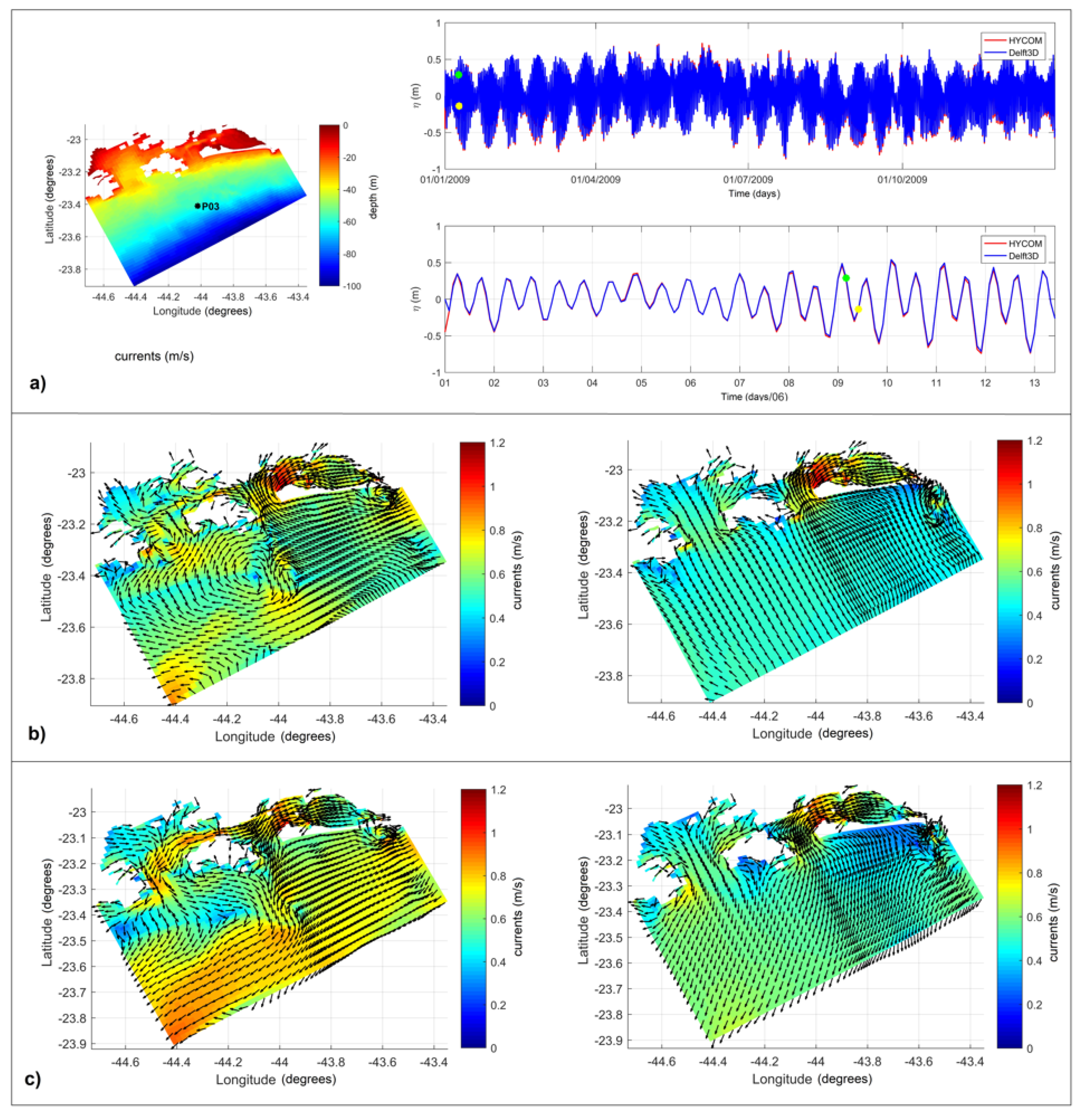
Figure 17. Comparison between Delft3D and HYCOM time series (a, on the right) for a central point in the computational mesh (a, on the left), focusing on the moments of flood (yellow dot) and ebb (green dot) used in the spatial representation of the Delft3D results with (on the left) and without (on the right) the meteorological signal for instants of flood (b) and ebb tide (c).

Figure 18. Spatial distribution of the difference between the time series of the Delft3D results with and without the meteorological signal for sea level (left) and current intensity (right).

Figure 19. Spatial variation of levels (on the left) and currents (on the right) of the Delft3D results for simulation considering only the M2 component with a lag of 1 min between the western and eastern borders for the following times from 09/19/2009 (from top to bottom): 2 h; 6 h; 10 h; 12 h.

Figure 20. Spatial variation of levels (on the left) and currents (on the right) of the Delft3D results for simulation considering only the M2 component with a lag of 4.92 h between the southern and northern borders for the following times from 09/19/2009 (from top to bottom): 2 h; 6 h; 10 h; 12 h.

Table 1. Total water volumes crossing the boundaries for the coastal (Delft3D) and ocean (HYCOM) models.

Boundary	HYCOM (m³)			Delft3D (m³)			Difference (m³)
Boundary	Volume out	Volume in	Residual	Volume out	Volume in	Residual	(V_HYCOM-V_Delft3D)
Western (wes)	1.65E+09	-1.78E+09	-5.24E+08	1.80E+09	-1.92E+09	-5.33E+08	9.20E+06
Southern (sou)	1.49E+09	-1.14E+09	4.51E+08	1.66E+09	-1.24E+09	5.40E+08	-8.88E+07
Eastern (eas)	9.06E+08	-8.96E+08	2.72E+08	8.34E+08	-8.45E+08	2.16E+08	5.62E+07
Grande I. (gra)	3.79E+07	-4.45E+07	-9.36E+06	1.54E+08	-1.34E+08	2.72E+07	-3.66E+07
Sepetiba I. (sep)	1.12E+07	-1.78E+07	-7.89E+06	1.04E+08	-1.08E+08	9.43E+06	-1.73E+07
Bacalhau (bac)	-	-	-	4.83E+04	-1.40E+05	-3.80E+04	3.80E+04
Total	4.10E+09	-3.88E+09	1.82E+08	4.55E+09	-4.24E+09	2.60E+08	-7.73E+07

Table 2. Initial and final volumes in the domain for the coastal (Delft3D) and ocean (HYCOM) models.

Measurements	HYCOM	Delft3D
Surface Area (m²)	1.38E+09	1.38E+09
Initial Volume (m³)	7.75E+10	7.83E+10
Final Volume (m³)	7.72E+10	7.80E+10
Difference (m³)	-2.35E+08	-3.23E+08

Table 3. Cross correlations of measured sea water level in Guanabara Bay (Ilha Fiscal station) and modeled for Sepetiba Bay (Guaíba Island station), after astronomical components removal.

Time interval	Length of series (months)	Cross correlation	Lag
jan/2009 to dec/2009	12	0.81	5h
jan/2009 to jun/2009	6	0.88	5h
jul/2009 to dec/2009	6	0.73	4h
jan/2009 to mar/2009	3	0.78	6h

Disclaimer/Publisher’s Note: The statements, opinions and data contained in all publications are solely those of the individual author(s) and contributor(s) and not of MDPI and/or the editor(s). MDPI and/or the editor(s) disclaim responsibility for any injury to people or property resulting from any ideas, methods, instructions or products referred to in the content.

© 2023 by the authors. Licensee MDPI, Basel, Switzerland. This article is an open access article distributed under the terms and conditions of the Creative Commons Attribution (CC BY) license (http://creativecommons.org/licenses/by/4.0/).

Copyright: This open access article is published under a Creative Commons CC BY 4.0 license, which permit the free download, distribution, and reuse, provided that the author and preprint are cited in any reuse.

MDPI Initiatives

Important Links

Choose an area of interest and we will send you notifications of new preprints at your preferred frequency.

Disclaimer