Quantitative Research of Cutoff Wavenumber and Wave Spectrum for Electromagnetic Scattering Computation with Two-Scale Method

Preprint

Article

Quantitative Research of Cutoff Wavenumber and Wave Spectrum for Electromagnetic Scattering Computation with Two-Scale Method

Altmetrics

Downloads

119

Views

Comments

This version is not peer-reviewed

Submitted:

16 December 2023

Posted:

18 December 2023

You are already at the latest version

Alerts

Abstract

The two-scale method (TSM) is an effective approach to simulate electromagnetic (EM) scattering from rough sea surface, to interpret physical interaction of EM wave with rough sea surfaces. The sea surface roughness spectrum and the cutoff wavenumber are two key factors affecting the accuracy of TSM simulation. This paper takes the geophysical model functions (GMFs) of different band as reference, and quantitatively studies the two factors based on the numerical simulation of different polarization backscattering coefficients. The numerical simulation demonstrates that Apel spectrum is more suitable for the backscattering simulation in C/X/Ku-band, and the optimal cutoff wavenumbers are also derived for TSM simulation of EM scattering in C/X/Ku-band. Then an empirical model function of optimal cutoff wavenumbers with respect to frequency, incident angle and wind speed are obtained with regression method. Finally, the simulation results with the new model function of cutoff wavenumber are compared with the GMF and measured data in different bands and they are all consistent. Moreover, a physical explanation for the optimal cutoff wavenumber is also given.

Keywords:

Subject: Environmental and Earth Sciences - Remote Sensing

1. Introduction

Ocean microwave remote sensing provides an important technology for global sea surface observation. Many scatterometers and radar missions have observed the ocean in space, such as Microwave Imaging Radiometer with Aperture Synthesis (MIRAS) on the ESA SMOS satellite, L-band microwave radiometer on NASA's Aquarius satellite, phased array L-band synthetic aperture radar (PALSAR) on Japan's ALOS satellite, Deutsche Aerospace's TerraSAR-X radar satellite and the microwave scatterometers on China's HaiYang-2 (HY-2) satellites. Based on certain inversion models, some marine environmental parameters, such as ocean wind vector, sea surface salinity/temperature, sea surface height, and so on, can be obtained from the observation data [1,2,3,4]. General, the inversion accuracy strictly relies on the electromagnetic (EM) scattering models of rough sea surfaces, which mainly include the empirical models and the physical models. The empirical models, generally called as geophysical model functions (GMF), are often obtained by fitting the observation data with the non-physical models, so they are limited by measurement geometry and physical mechanisms [5,6]. Therefore, it’s necessary to establish a physical model in line with real marine environments according to EM scattering mechanism.

Among the existing rough sea surface scattering models, the two-scale method (TSM) is widely used due to its ability to simultaneously consider the scattering contributions of both large-scale and small-scale roughness [4,6,7,8]. However, it’s well known that the simulation accuracy of TSM mainly depends on the input models, such as seawater permittivity, roughness spectrum of sea surface and cutoff wavenumber.

Most classical permittivity models were developed based on Debye model and measured data. Meissner and Wentz (2004) combined their measurements and the observation data of Special Sensor Microwave/Imager (SSM/I) to fit the Debye relaxation parameter of the seawater permittivity by minimizing the total error between the observations and the model calculations [9]. Furthermore, Meissner et al. improved the fitting model in 2012 by combining WindSat measurements at C-band and X-band [10]. Zhou et al. (2021) developed the GW2020 model based on the measurement with the resonance method [11]. Since these models are fitted based on specific observation data, they all have their own applicable ranges. So, we will sift a suitable one from the existing models [4,9,10,11,12] for TSM computation.

The sea spectrum is another important input for TSM computation. Researchers have developed many roughness spectrums based on experimental data, wave formation mechanism and scattering/radiation data. For example, Pierson and Moskowitz developed the first reliable PM wave spectrum according to the data of the North Atlantic experiment. The PM spectrum describes a fully developed sea surface, that is, it describes stable and uniform wind-driven waves on infinite sea surface, and there is a balance between input and dissipation of each wavelength [13]. As the fully developed wind wave is an ideal concept, researchers further developed JONSWAP spectrum, Phillips spectrum and so on based on PM spectrum and experimental data [6]. However, these spectrums only describe the gravity wave accurately and are only suitable for EM scattering simulation of sea surface in some frequency bands. In 1979, Bjerkaas and Riedel put forward the first full wavenumber BR spectrum by connecting four independent wavenumber ranges including gravity wave, short gravity wave, gravity capillary wave and capillary wave [14]. Since the arbitrary constants used to connect independent bands in BR spectrum have no physical significance, researchers later proposed Durden-Vesecky spectrum, Apel spectrum, Elfouhaily spectrum, KHCC03 spectrum [15], etc. Elfouhaily et al. also developed a unified angular spread function as they thought that the Fourier transform of the real even spreading function in the sea spectrum should have the characteristics of central symmetry [16]. Moreover, Hwang et al. proposed a series of H spectrum models by inverting the polarized echo data (scattering cross-section and emissivity data) to obtain the short-scale properties of the ocean surface [17]. Until now, numerous spectrum models have been proposed to describe the sea surface geometry, but none of these spectra has been proven suitable for EM scattering simulation in full frequency band, full polarization and full sea state [6]. In this paper, three commonly used spectrums, including DV spectrum [18], Apel spectrum [19] and Elfouhaily spectrum, are analyzed for backscattering computation.

The TSM algorithm divides the sea surface spectrum into large- and small- scales, with Kirchhoff approximation (KA) for large-scale scattering contribution and small perturbation method (SPM) for small-scale part. Therefore, the value of cutoff wavenumber for division of large-scale and small-scale spectrum is crucial for the scattering results. Some researchers empirically selected the cutoff wavenumber according to the scattering characteristics in different situations [18,20,21], but these empirical cutoff wavenumbers are always limited to specific conditions. As early as 1987, Guissard and Sobieski proposed a cutoff wavenumber criterion that varies with frequency and roughness spectrum by simplifying the applicability conditions for large-scale and small-scale surfaces [22]. Then, this criterion was used by Liu et al. in FASTEM-4 [4]. Furthermore, Li et al. (2020) proposed an adaptive cutoff wavenumber by making the measured sea surface roughness equal to the root mean square height of the small-scale sea surface spectrum [23]. Based on the assumption that the physical optical integral is asymptotically "α-stable distribution" under high frequency limit conditions, Johnson et al. (2022) proposed a cutoff wavenumber model that depends on frequency, spectrum, and incident angle. They have proved that this method can improve the consistency between geometric optical prediction and small slope approximation under some incident conditions [24]. But there is still no comprehensive evaluation of these methods.

In this paper, seawater permittivity, sea spectrum and cutoff wavenumber are studied for exact EM scattering computation with TSM. The paper is organized as follows. Section 2 describes the principle of TSM. Section 3 discusses the selection of the input models in TSM. The model of seawater permittivity is determined by comparing four different models. With the corresponding GMFs as reference (CMOD7 in C-band [25], XMOD2 in X-band [1] and NSCAT-4 in Ku-band [26]), the optimal cutoff wavenumbers and the most suitable spectrum are obtained. Then the fitting functions of the optimal cutoff wavenumber with respect to radar parameters and wind speed are obtained by multiple regression analysis. In Section 4, the simulation results using Apel spectrum and different cutoff wavenumber models are compared with GMFs and Haiyang-2 satellite data to evaluate the fitting functions. Section 5 gives some conclusions.

2. The Theory of Two-Scale Method

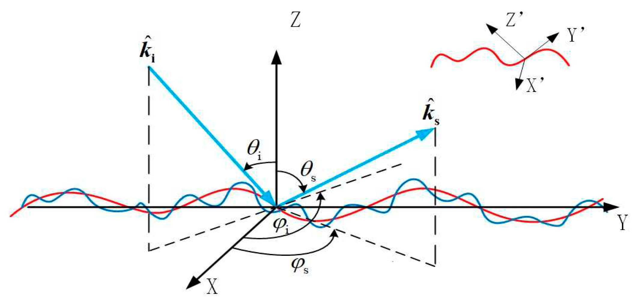
TSM was first proposed by Wentz et al. to expand the application scope by combining KA and SPM [20]. It treats the sea surface as a composite model, with a small-scale fluctuation superimposed on a large-scale fluctuation (Figure 1). The Kirchhoff approximation and geometric optical (KA-GO) method is used to solve EM scattering of the large-scale rough surface, and the backscattering coefficient is expressed as [27]

γ^{KA - GO} = \frac{{|R (0)|}^{2}}{2 \cos^{4} θ_{i} s_{u} s_{c}} \exp (- \frac{\tan^{2} θ_{i}}{2 s_{u} s_{c}}),

(1)

Here

R (0)

stands for the Fresnel reflection coefficient at normal incidence,

s_{u}

s_{c}

respectively represent the root mean square slope in upwind and crosswind directions.

Figure 1. The two-scale model of electromagnetic scattering from rough sea surface.

The SPM is used to solve EM scattering of the small-scale rough surface. Because of the variance of local incident angle caused by the large-scale surface slope, the horizontal and vertical polarization backscattering coefficients in local coordinate system are expressed as

{γ^{'}}_{aa}^{SPM} = 4 π k_{i}^{2} \cos^{4} θ_{il} {|f_{aa}|}^{2} W_{s} (2 k_{i} \sin θ_{il}),

(2)

f_{hh} = - \frac{2 k_{i} (ε_{r} - 1)}{{(\cos θ_{il} + \sqrt{ε_{r} - \sin^{2} θ_{il}})}^{2}},

(3)

f_{vv} = \frac{2 k_{i} (ε_{r} - 1) [ε_{r} + (ε_{r} - 1) \sin^{2} θ_{il}]}{{(ε_{r} \cos θ_{il} + \sqrt{ε_{r} - \sin^{2} θ_{il}})}^{2}},

(4)

Here

θ_{il}

is local incident angle caused by the large-scale surface slope,

W_{s} = W (k_{ρ} > k_{c})

represents the small-scale roughness spectrum,

k_{c}

is the cutoff wavenumber,

k_{ρ}

is the spatial wave number of ocean waves,

k_{i}

is the incident wave number,

ε_{r}

represents the relative permittivity of seawater. Since the above SPM formulas are expressed in the local coordinate system, the following polarization transformation is needed.

[\begin{array}{l} \begin{matrix} S_{hh} & S_{hv} \end{matrix} \\ \begin{matrix} S_{vh} & S_{vv} \end{matrix} \end{array}] = [\begin{array}{l} \begin{matrix} {\hat{h}}_{s} \cdot {\hat{h}}_{sl} & {\hat{h}}_{s} \cdot {\hat{v}}_{sl} \end{matrix} \\ \begin{matrix} {\hat{v}}_{s} \cdot {\hat{h}}_{sl} & {\hat{v}}_{s} \cdot {\hat{v}}_{sl} \end{matrix} \end{array}] [\begin{array}{l} \begin{matrix} {S^{'}}_{hh} & {S^{'}}_{hv} \end{matrix} \\ \begin{matrix} {S^{'}}_{vh} & {S^{'}}_{vv} \end{matrix} \end{array}] [\begin{array}{l} \begin{matrix} {\hat{h}}_{il} \cdot {\hat{h}}_{i} & {\hat{h}}_{il} \cdot {\hat{v}}_{i} \end{matrix} \\ \begin{matrix} {\hat{v}}_{il} \cdot {\hat{h}}_{i} & {\hat{v}}_{il} \cdot {\hat{v}}_{i} \end{matrix} \end{array}],

(5)

where

\hat{h}

\hat{v}

are horizontal and vertical polarization. The subscript

l

represents the local coordinate system,

i

and

s

represent the incident and scattering directions, respectively.

{S^{'}}_{ab}

S_{ab}

represent the scattering amplitude in the local coordinate system and the globe coordinate system. The relationship between

S_{ab}

and

γ_{ab}

γ_{ab} = 4 π < {|S_{ab}|}^{2} >,

(6)

here

< \cdot >

stands for set averaging. The amplitude of

{S^{'}}_{a b}

can be obtained by (2) and (6). A random phase, uniformly distributed in

[- π, π]

, is often added to represent the phase of

{S^{'}}_{ab}

[28]. Once the

{S^{'}}_{ab}

is obtained, we can use (5) and (6) to get the scattering coefficients in the globe coordinate system

γ_{ab}^{SPM}

. Finally, according to the tilt modulation of large-scale surface, the backscattering coefficient of TSM is written as

\begin{array}{l} γ_{ab}^{TSM} (θ_{s}, φ_{s}; θ_{i}, φ_{i}) = γ_{ab}^{KA - GO} (θ_{s}, φ_{s}; θ_{i}, φ_{i}) + \\ \int_{- \infty}^{\infty} d {s'}_{y} \int_{- \cot θ_{i}}^{\infty} d {s'}_{x} [γ_{ab}^{SPM} (θ_{sl}, φ_{sl}; θ_{il}, φ_{il}) (1 - {s'}_{x} \tan θ_{i}) p (s_{x}, s_{y})] \end{array},

(7)

Here

p (s_{x}, s_{y})

is the distribution function of large-scale slope.

s_{x}

s_{y}

are the slopes along

x

and

y

axes in the principle system, and

{s'}_{x}

{s^{'}}_{y}

are the slopes in the observation system of radiometer.

3. Key factors of TSM Model

3.1. Permittivity model of Seawater

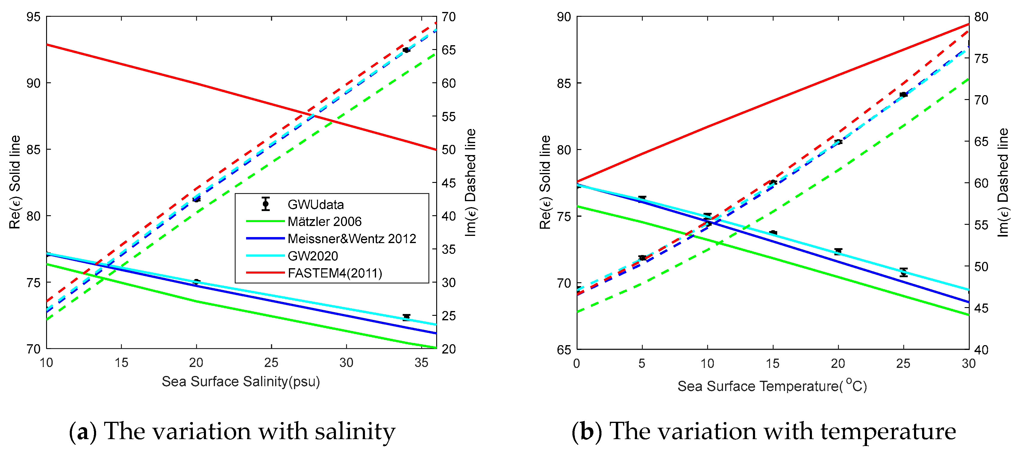
As one of the inputs to the scattering model of TSM, the seawater permittivity model needs to reflect the real marine environment, so as to get more exact scattering results. At present, a variety of seawater permittivity models suitable for different temperatures and salinities have been developed based on the measurement data [4,9,10,11,12]. Figure 2 compares four models with the experimental data presented by Zhou et al. (2021). The real part of FASTEM4 model developed by Liu et al. (2011) [4] always deviates significantly from the experimental data, whether changing seawater temperature or salinity. The GW2020 model is the most consistent with the data, and it is selected as the input of the scattering model in the following.

The GW2020 model was developed by Zhou et al. for the Aquarius satellite mission to create a global salinity distribution map. Utilizing measurement data acquired through a resonant cylindrical microwave cavity in transmission mode, they fitted the coefficients in the single Debye model. The expression of the model is as follows [11]

ε_{r} (S, T) = 4.9 + \frac{ε_{s} (T) r (S, T) - 4.9}{1 + j 2 π f τ (T)} - j \frac{δ (S, T)}{2 π f ε_{0}},

(8)

Here

ε_{0}

is the vacuum permittivity,

f

is the frequency of incident EM wave (Hz),

ε_{s} (T)

is the static permittivity of pure water (

f = 0

δ (S, T)

is the conductivity of seawater,

τ (T)

is Debye relaxation time,

T

is the sea surface temperature (

℃

S

is the sea surface salinity (psu). These specific Debye parameter forms are fitted as follows with the measured data.

τ (T) = 1.7503 \times 10^{- 11} - 6.1299 \times 10^{- 13} T + 1.2451 \times 10^{- 14} T^{2} - 1.1493 \times 10^{- 16} T^{3},

(9)

ε_{s} (T) = 88.052 - 4.0179 \times 10^{- 1} T - 5.1027 \times 10^{- 5} T^{2} + 2.5589 \times 10^{- 5} T^{3},

(10)

\begin{matrix} r (S, T) = 1 - 3.9719 \times 10^{- 3} S + 2.4921 \times 10^{- 5} S \cdot T + 4.2756 \times 10^{- 5} S^{2} \\ - 3.9283 \times 10^{- 7} S^{2} \cdot T - 4.1535 \times 10^{- 7} S^{3} \end{matrix},

(11)

\begin{matrix} δ (S, T) = (9.5047 \times 10^{- 2} S - 4.3086 \times 10^{- 4} S^{2} + 2.1618 \times 10^{- 6} S^{3}) \\ \times (1 + 3.7602 \times 10^{- 2} T + 6.3283 \times 10^{- 5} T^{2} + 4.8342 \times 10^{- 7} T^{3} \\ - 3.9748 \times 10^{- 4} S \cdot T + 6.2652 \times 10^{- 6} S^{2} \cdot T) \end{matrix} .

(12)

3.2. Spectrum Model of Rough Sea Surface

General, the expression of sea spectrum can be written as [16]

W (k_{ρ}, φ) = \frac{1}{k} S (k_{ρ}) ϕ (k_{ρ}, φ),

(13)

Here

S (k_{ρ})

describes the one-dimensional omnidirectional wave spectrum,

ϕ (k_{ρ}, φ)

is the spreading function that describes the dependence of wind direction. The relationship between one-dimensional omnidirectional spectrum

S (k_{ρ})

and wave spectrum is expressed as

S (k_{ρ}) = \int_{- π}^{π} W (k_{ρ}, φ) k_{ρ} d φ .

(14)

Based on the Bragg scattering mechanism, the accuracy of TSM simulation depends on the accurate statistical description of the sea surface topography in the range from gravity waves to capillary gravity waves. Many experiments have measured the wind-induced gravity spectrum, but these measurements are only applicable to certain ocean conditions and sea areas. And it is often very difficult to measure the undulating height of sea surface by situ experiments, especially the short-wave part. Up to now, no experiment has been carried out to measure the spectrum of the whole wavelength at the same time. So, there is still no universally accepted spectrum model for EM scattering computation and inversion of ocean parameters [5,6].

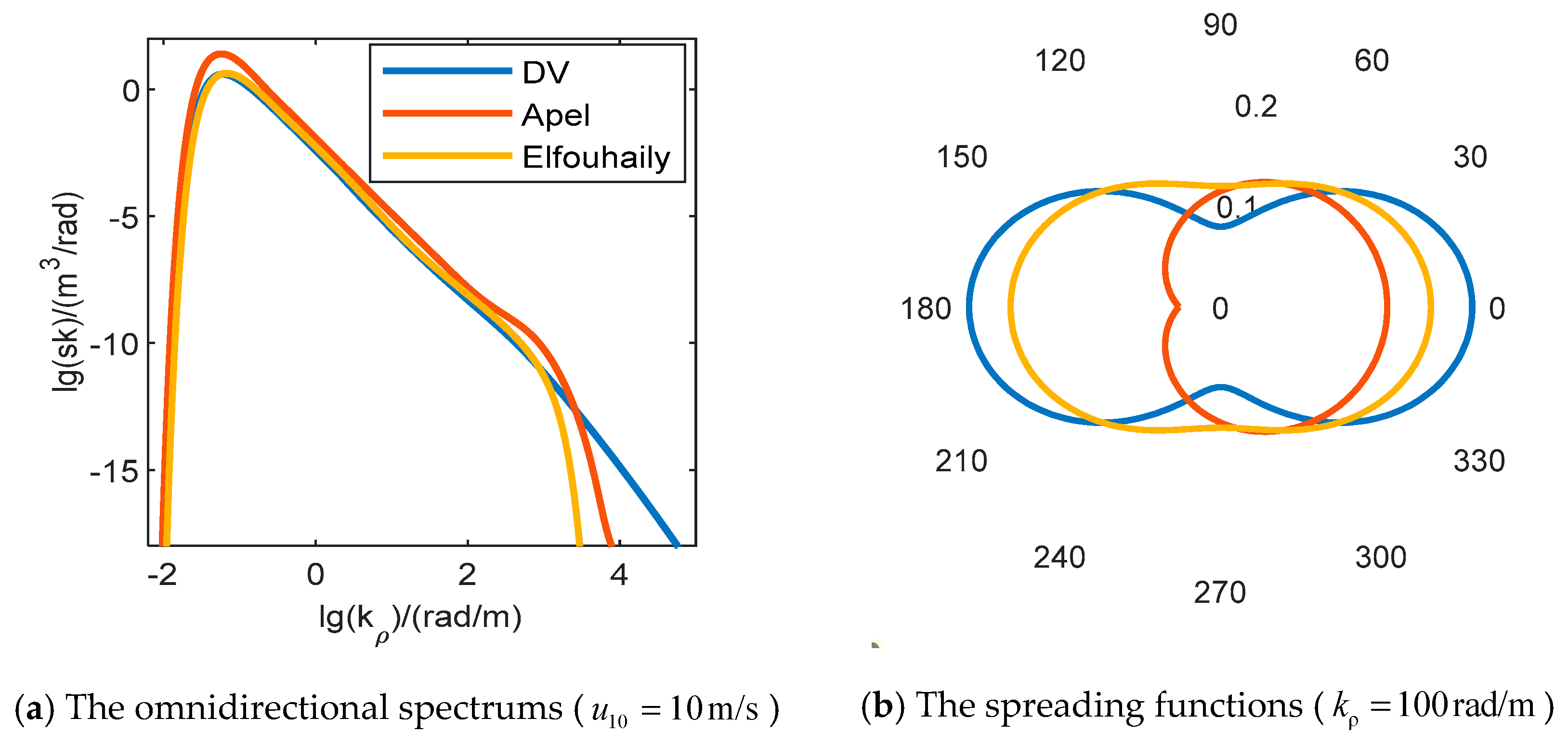
Since no sea surface roughness spectrum can be used for all frequency and all polarization simulation, the spectrums suitable for different conditions should be studied [5]. In this paper, several commonly used spectrums: DV spectrum, Apel spectrum and Elfouhaily spectrum are employed to investigate their applicability for TSM simulation at different conditions. The details are in Appendix A, B and C. According to (13) and (14), the integral of

ϕ (k_{ρ}, φ)

at (

- π ~ π

) should be equal to 1, while the integrals of the original spreading functions of DV spectrum and Apel spectrum in this interval are

2 π

. Based on this analysis, the spreading functions of these two spectrums are normalized in this paper, and the omnidirectional spectrum of Apel spectrum is modified by combining (13) and the normalized spreading function. Figure 3 compares these three spectrums. Figure 3(a) shows three omnidirectional spectrums at wind speed of 10 m/s, and the difference is mainly focused on the description of the shortwave part. Figure 3(b) shows the directional transfer functions of these three spectrums at

k_{ρ} = 100 r a d / m

. The spreading function of Apel spectrum is asymmetric and can be used for Doppler spectrum simulation of radar reflected signals which require an asymmetric spreading function [6]. While the spreading functions of DV and Elfouhaily spectrum are centrally symmetric and they are analytically suitable for EM models. The distribution of these three spectrums under other wind speed or wave number values is similar to Figure 3.

3.3. Effect of Different Cutoff Wavenumbers

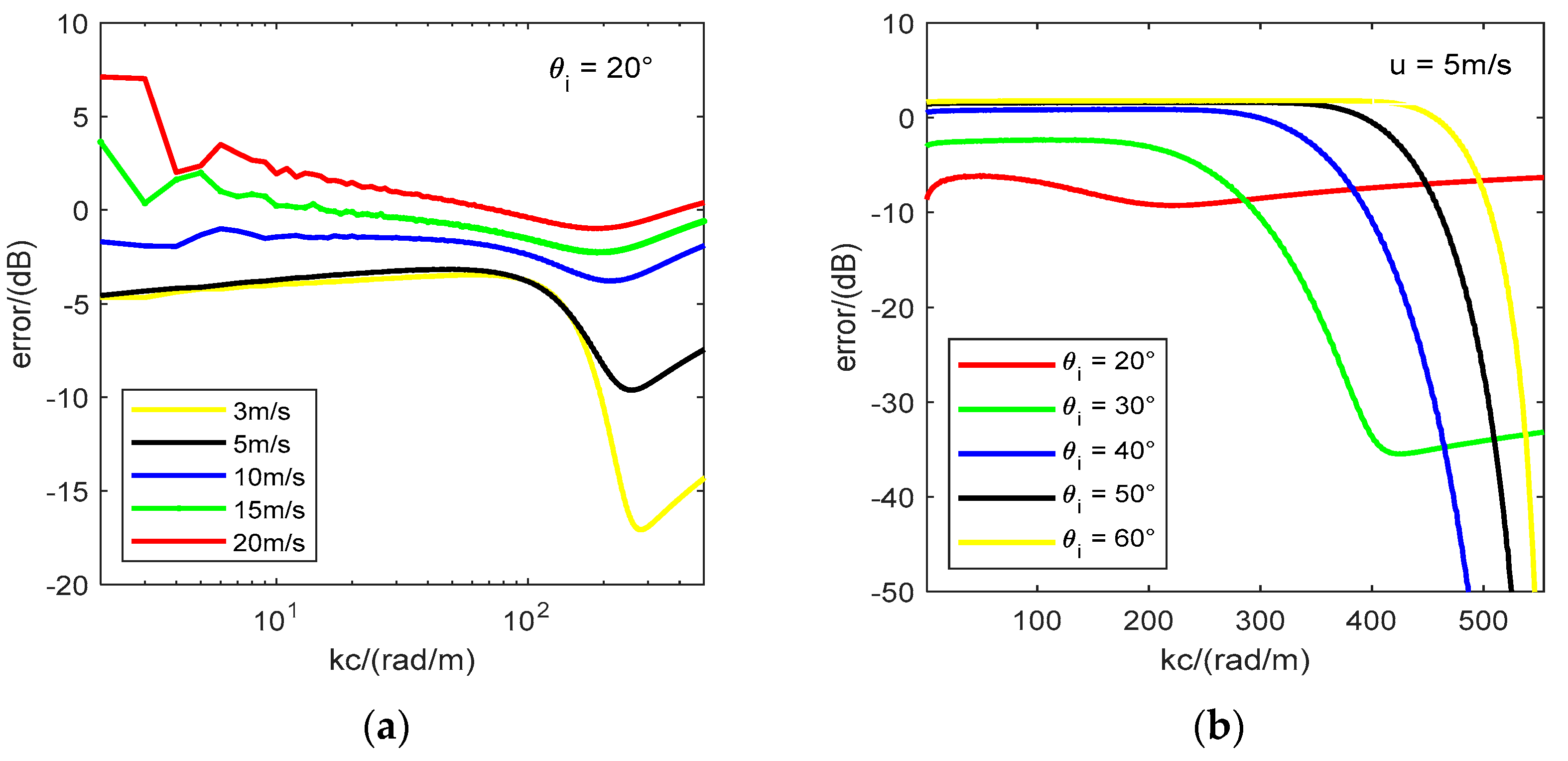
For TSM simulation, the cutoff wavenumber used to divide the large-scale and small-scale spectrum is also an important factor. Even for the same sea spectrum and the same incident wave parameters, different cutoff wavenumbers will infer different scattering calculation results. Taking the scattering calculation in Ku-band as example, Figure 4 shows the difference of backscattering coefficients between TSM simulation results and the NSCAT-4 model when the cutoff wavenumber takes different values. Here we used the DV spectrum describing the sea surface geometry. The error varies obviously with the cutoff wavenumber. And the values of the black line and the yellow line in Figure 4(a) are always less than 4dB while a cutoff wavenumber can be found in other lines to make the error about 1dB. This observation suggests that DV spectrum may be not suitable for the backscattering simulation of TSM in Ku-band when the wind speed is less than 5 m/s.

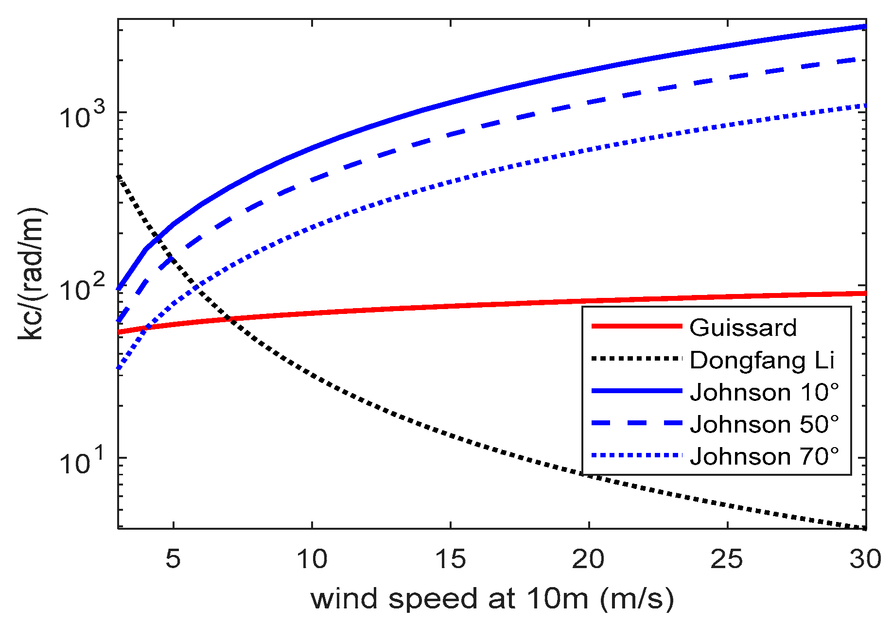
Since TSM simulation results of different cutoff wavenumbers are different, it is necessary to study an approximate cutoff wavenumber to improve the accuracy of TSM simulation. Several cutoff wavenumber models have been proposed [22,23,24]. Since Li's model does not vary with frequency, the three models are compared in the Ku-band and the frequency is 13.256 GHz. Figure 5 shows the results of these models for the division of DV spectrum. The red line and black line respectively show the results of Guissard criterion and Li’s model with wind speed, and the three blue lines show Johnson’s model at different incident angles. The cutoff wavenumbers given by different models vary greatly under the same incident conditions, so it’s essential to delve into the discussion of cutoff wavenumber next.

3.4. The Selection of Spectrum and Cutoff Wavenumber

To validate the accuracy of a model, researchers often compare the simulation results of the scattering model with the empirical GMF, which describes a direct relationship between backscattering cross section and marine physical parameters. A GMF is firstly established qualitatively according to the variation trend of scatterometer data with physical parameters. Then the coefficients are determined quantitatively by fitting methods such as least square. General, the GMF is related to frequency, incident angle, polarization

p

, wind speed

u

and relative wind direction [27], where the relative wind direction is defined as the difference of the wind direction azimuth minus the scatterometer observation azimuth. Since GMFs do not have a clear physical mechanism, it is usually used to verify the theoretical simulation model of sea surface microwave scattering. In the following, the CMOD7 in C-band [25], XMOD2 in X-band [1] and NSCAT-4 in Ku-band [26] are used for comparison. Using the corresponding GMF model as reference, the optimal cutoff wavenumbers will be determined to minimize the absolute error

|γ_{TSM} - γ_{GMF}|

for different frequency and incident conditions. Since CMOD7 in C-band and XMOD2 in X-band only work at VV polarization, we employ the polarization ratio (PR) model to obtain HH polarization in these two bands. The PR model is defined as following

PR = \frac{γ_{vv}}{γ_{hh}} .

(15)

The PR model used in C-band is expressed

PR_c = 0.453041 \times \exp (0.032457 θ_{i}) + 0.524303 .

(16)

For the PR model used in X-band, we adopt the model proposed by Shao et al. in 2016, which incorporates both incidence angle and sea surface wind speed [29]. The expression of this model is

PR_x = (0.0011 θ_{i}^{2} - 0.0615 θ_{i} + 1.9581) \cdot u_{10}^{(0.0082 θ_{i} - 0.2308)} .

(16)

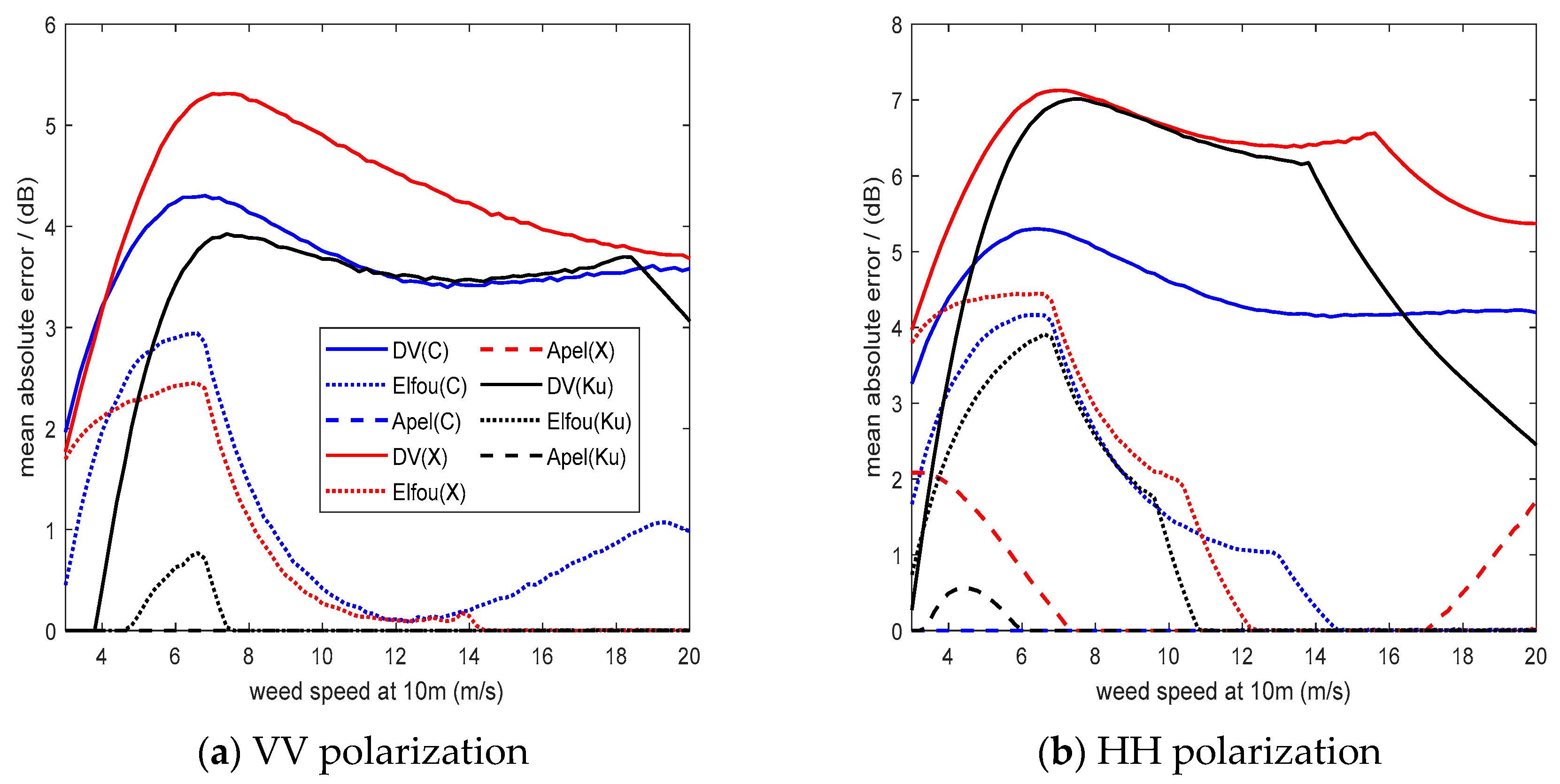
Figure 6 shows the minimum absolute errors of different spectrums, when the incident direction is

θ_{i} = 30 °

φ_{i} = 90 °

and the frequencies are 5.255 GHz (C-band), 9.65 GHz (X-band) and 13.256 GHz (Ku-band) respectively. For VV polarization, the simulation errors of Apel spectrum at corresponding optimal cutoff wavenumbers are always the smallest. What’s more, we also compared the minimum absolute errors at other incident condition (wind speed of 3~20 m/s, the incident angle of 30°~66°, and the azimuth angle of 0°~180°) and found that the Apel spectrum has the smallest error at VV polarization. These results demonstrate that a suitable

k_{c}

can always be found to make the simulation result of Apel spectrum exactly equal to the GMF result. In the case of HH polarization, the minimum error between the simulation results of Apel spectrum and GMF is mostly between 0~3dB when the wind speed

u_{10} > 15

m/s. Therefore, the applicable range of wind speed for Apel spectrum is adjusted to 3~15m/s at HH polarization.

Since the incident angle ranges of GMFs used in this paper are different, Table 1 gives the applicable incident angle ranges suitable for simulating with the Apel spectrum in different frequency bands. The lower limit is chosen because when the incident angle is less than 30°, the minimum error between the simulation results of Apel spectrum and GMF is mostly between 2~3dB. We analyzed that the reason may be that KA-GO plays a dominant role in the two-scale model when the incident angle is less than 30°. It can be observed from Equation (3) that

γ^{KA - GO}

is a function of root mean square slope of upwind and crosswind. However, the slopes change relatively slowly with the cutoff wavenumber and the KA-GO simulation results only depend weakly on the selected cutoff wavenumber [24]. It’s not feasible to improve TSM simulation results by adjusting the cutoff wavenumber when incident angles are less than 30°.

3.5. Empirical Function of Optimal Cutoff Wavenumber

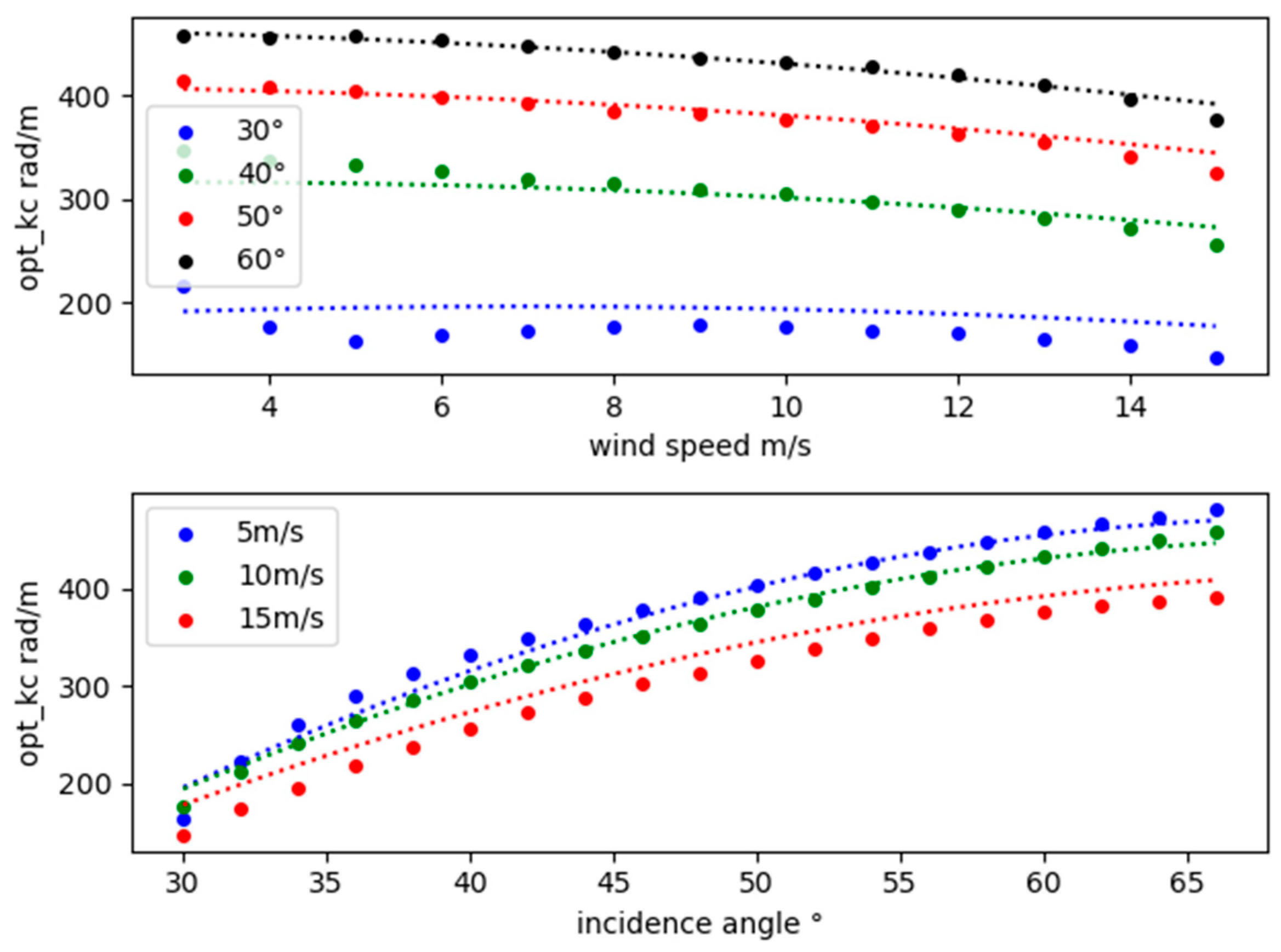
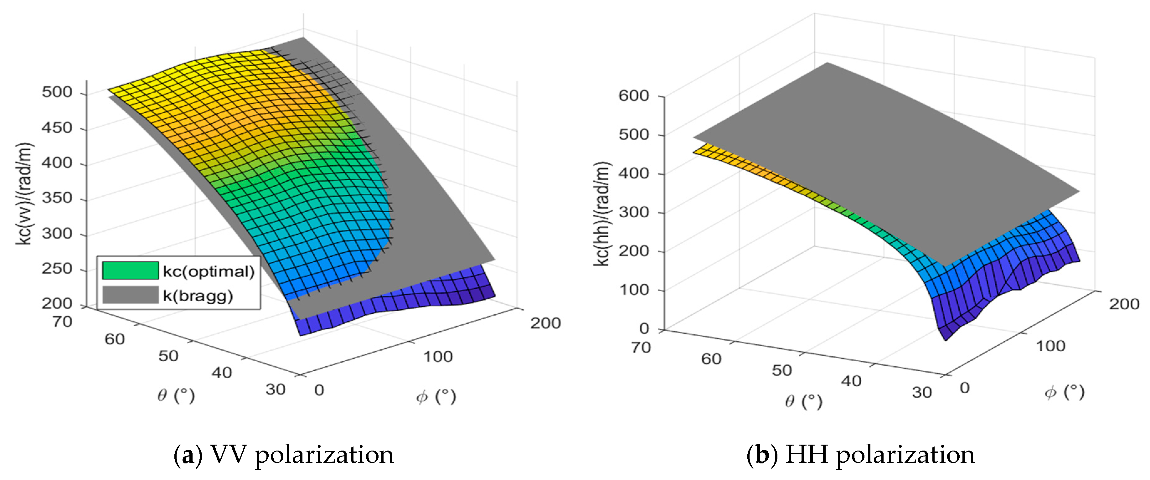
The above analysis indicates that the optimal cutoff wavenumber is related to multiple parameters. For ease of use, a functional relationship of cutoff wavenumber vs. wind speed, frequency, incident angle and azimuth angle will be fitted using the multiple linear regression method in this section. Figure 7 shows the optimal cutoff wavenumbers of Apel spectrum in Ku-band vs. incident angle and azimuth angle when the wind speed

u_{10} = 5

m/s. The gray surface represents the Bragg wavenumber (

k_{b} = 2 k \sin θ_{i}

). The trend of the optimal cutoff wavenumber is basically consistent with the gray surface. Besides, Figures 7(a) and 7(b) illustrate that the optimal cutoff wavenumbers vary for different polarizations. Therefore, we have fitted the empirical functions of cutoff wavenumber for VV and HH polarizations respectively.

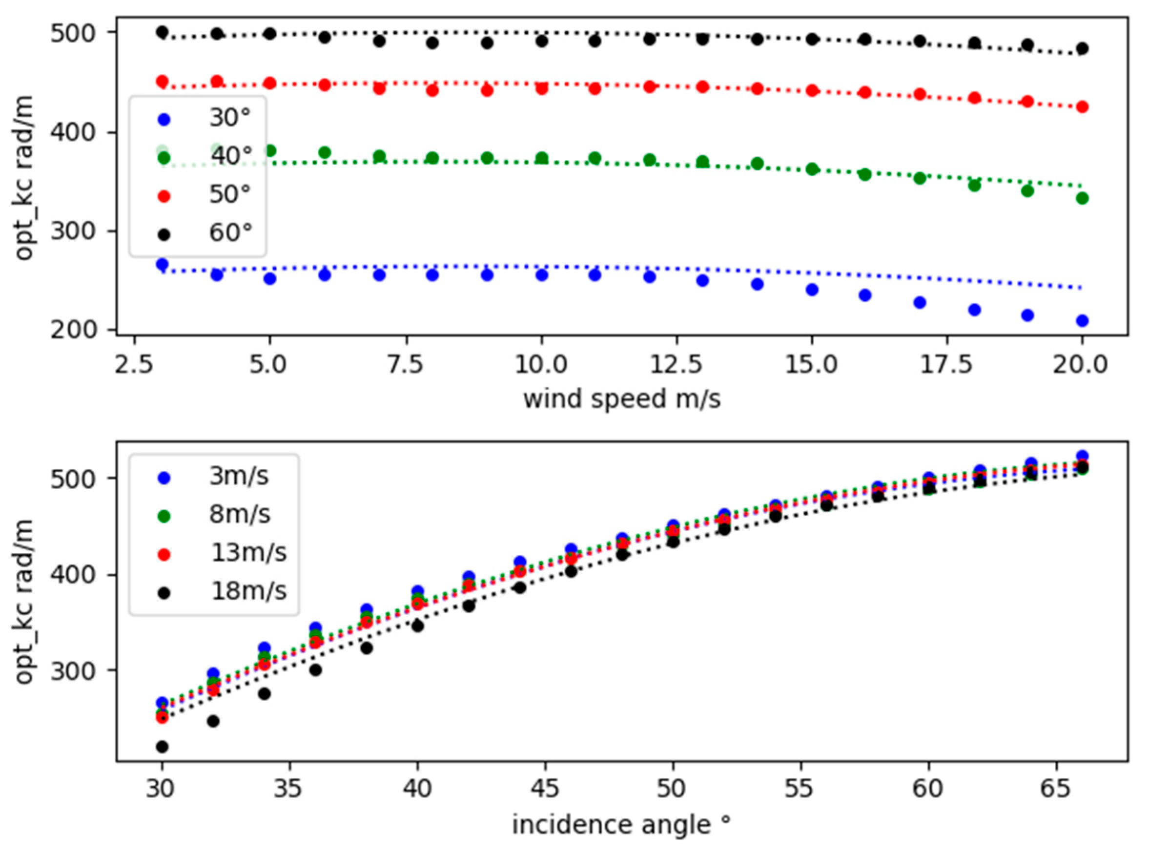
Based on the Bragg scattering mechanism and the dependence on azimuth angle of GMF [1], [25,26], we choose the trigonometric functions of incident angle and azimuth angle as the basic functions of linear regression model [31]. Then the n-order polynomial of six basis functions is generated as

{(k + u_{10} + \sin θ_{i} + \cos θ_{i} + \sin φ_{i} + \cos φ_{i})}^{n}

(n=1~6). The ridge regression model with L2 regularization is used to obtain the coefficients [31]. Four regression evaluation indicators, including mean squared error (MSE), root mean squared error percentage (RMSE%), R-squared score (r2_score) and explained variance score (EVS), are used to evaluate the performance of regression, as shown in Figure 8 and Figure 9, and the abscissa is the number of terms in n-order polynomial. Figure 8 indicates that the number of the polynomial terms increases sharply with the increase of the order. However, when the order is greater than 3, increasing the order of polynomial does not significantly reduce the mean squared error. This means that there may be many irrelevant redundant features in higher-order polynomial, which may lead to over-fitting. Considering the complexity of the cutoff wavenumber empirical function and the four evaluation indexes (as shown in Figure 8), we finally use the second-order polynomial to make regression analysis.

Table 2 gives the terms and their coefficients in the second-order polynomial fitting function for VV polarization optimal wavenumber in C-, X- and Ku-bands. The four evaluation indexes of this regression model are MSE=51.199, RMSE%= 0.027, r2_score = EVS = 0.997. Figure 10 gives the comparison between the fitted empirical function (dotted line) and the original data (dot). The fitting model is basically consistent with the data.

Table 2. Terms and coefficients of the empirical function for vertical polarization optimal wavenumber in C-, X- and Ku-bands.

	Term	Coefficient		Term	Coefficient		Term	Coefficient
1	$k$	-2.747	10	$k \sin θ_{i}$	3.248	19	$\cos θ_{i} \sin θ_{i}$	16.530
2	$u_{10}$	8.638	11	$k \cos φ_{i}$	0.060	20	$\cos θ_{i} \cos φ_{i}$	45.798
3	$\cos θ_{i}$	-28.403	12	$k \sin φ_{i}$	0.042	21	$\cos θ_{i} \sin φ_{i}$	34.490
4	$\sin θ_{i}$	37.915	13	$u_{10}^{2}$	-0.169	22	$\sin θ_{i} \cos φ_{i}$	41.850
5	$\cos φ_{i}$	-69.707	14	$u_{10} \cos θ_{i}$	-5.178	23	$\sin θ_{i} \sin φ_{i}$	-17.445
6	$\sin φ_{i}$	-23.356	15	$u_{10} \sin θ_{i}$	-5.127	24	$\cos 2 φ_{i}$	-7.696
7	$k^{2}$	0.003	16	$u_{10} \cos φ_{i}$	0.036	25	$\cos φ_{i} \sin φ_{i}$	10.271
8	$k u_{10}$	0.002	17	$u_{10} \sin φ_{i}$	1.507	26	1	56.343
9	$k \cos θ_{i}$	1.127	18	$\cos 2 θ_{i}$	-6.875

Figure 10. Comparison between empirical function and data at VV polarization (

φ_{i} = 30 °

f = 13.256 GHz

Figure 10. Comparison between empirical function and data at VV polarization (

φ_{i} = 30 °

f = 13.256 GHz

For HH polarization, we still conducted a regression analysis using a second-order polynomial for the optimal cutoff wavenumber data obtained from the Apel spectrum in the Ku-band. Table 3 gives the terms and their coefficients in the second-order polynomial fitting function for HH polarization optimal wavenumber in C-, X- and Ku-band. The four evaluation indexes of this regression model are MSE=152.517, RMSE%=0.053, r2_score = EVS = 0.991. Figure 11 gives the comparison between the fitted empirical function (dotted line) and the original data (dot). It can see that the fitting model is basically consistent with the data in most cases. But there are also some cases where the empirical model overestimates the cutoff wavenumber (

θ_{i} = 30 °

). And the empirical function range for the cutoff wavenumber in HH polarization is adjusted to 3~15 m/s as the minimum error between the HH polarization simulation results of Apel spectrum and GMF is mostly between 0~3dB when the wind speed

u_{10} > 15

m/s. To further access the accuracy of the empirical models given in Table 2 and Table 3, both models will be brought into TSM for verification in the following.

Table 3. Terms and coefficients of the empirical function for horizontal polarization optimal wavenumber in C-, X- and Ku-bands.

	Term	Coefficient		Term	Coefficient		Term	Coefficient
1	$k$	-4.111	10	$k \sin θ_{i}$	4.282	19	$\cos θ_{i} \sin θ_{i}$	52.002
2	$u_{10}$	32.072	11	$k \cos φ_{i}$	0.113	20	$\cos θ_{i} \cos φ_{i}$	34.884
3	$\cos θ_{i}$	-4.257	12	$k \sin φ_{i}$	-0.017	21	$\cos θ_{i} \sin φ_{i}$	26.527
4	$\sin θ_{i}$	38.190	13	$u_{10}^{2}$	-0.266	22	$\sin θ_{i} \cos φ_{i}$	28.048
5	$\cos φ_{i}$	-62.579	14	$u_{10} \cos θ_{i}$	-15.855	23	$\sin θ_{i} \sin φ_{i}$	19.327
6	$\sin φ_{i}$	-42.113	15	$u_{10} \sin θ_{i}$	-27.360	24	$\cos 2 φ_{i}$	-11.624
7	$k^{2}$	0.004	16	$u_{10} \cos φ_{i}$	-0.135	25	$\cos φ_{i} \sin φ_{i}$	9.809
8	$k u_{10}$	-0.010	17	$u_{10} \sin φ_{i}$	2.918	26	1	43.345
9	$k \cos θ_{i}$	1.215	18	$\cos 2 θ_{i}$	44.469

Figure 11. Comparison between empirical function and data at HH polarization (

φ_{i} = 30 °

f = 13.256 GHz

Figure 11. Comparison between empirical function and data at HH polarization (

φ_{i} = 30 °

f = 13.256 GHz

4. Comparison and Discussion

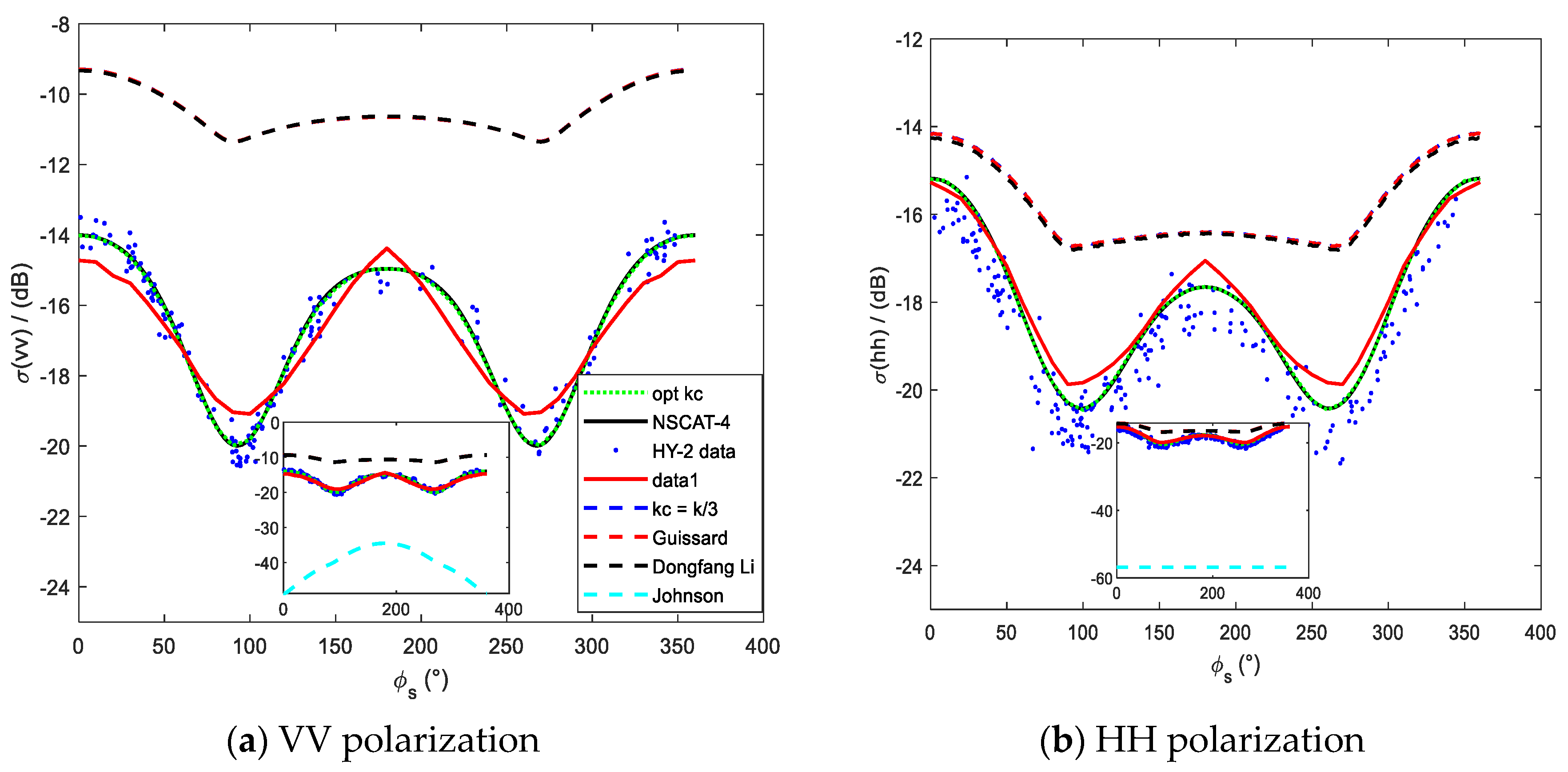
To further illustrate that the TSM backscattering simulation of Apel spectrum can be improved with the appropriate cutoff wavenumber, the simulation results in C-, X- and Ku-bands with different cutoff wavenumber models are compared. The results are also compared with the corresponding GMFs in these bands. Moreover, the HY-2 satellite data (backscattering cross section products of orbit-17453 on 2022, Apr.17, 18:53~20:38) provided by the China Ocean Satellite Service System is used for comparison in Ku-band.

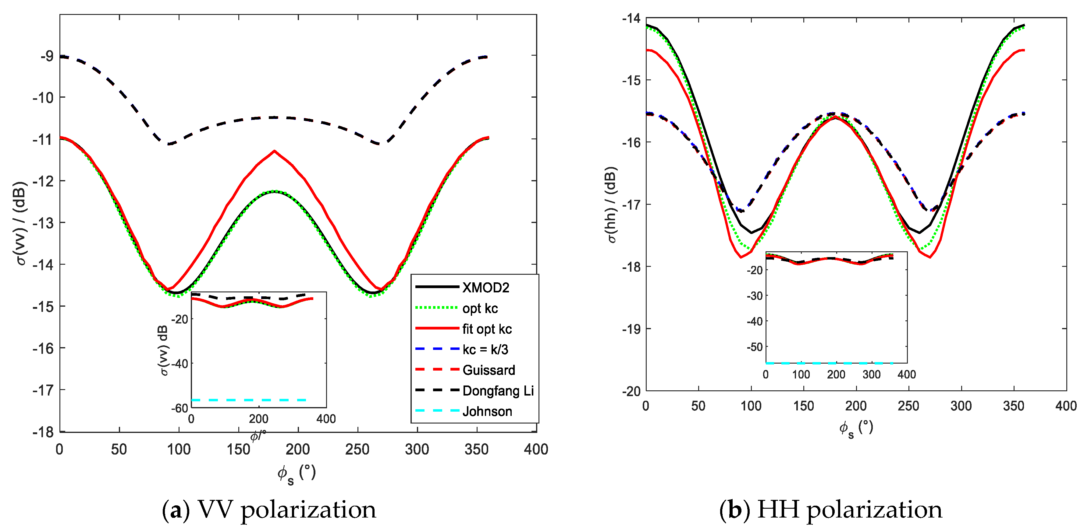
Figure 12, 13 and 14 show the comparison results of backscattering coefficients as a function of scattering azimuth in C-, X- and Ku-bands respectively. The black solid line represents the simulation results of GMFs model, the red solid line represents the TSM simulation results using the cutoff wavenumber given by our empirical function, and the green dotted line represents the TSM simulation results with the optimal cutoff wavenumber data. The dashed lines show the results of other cutoff wavenumber models. In comparison with the dashed lines, the simulation results with our cutoff wavenumber model are more consistent with the GMFs. The slight difference between the green dotted line and red solid line is due to the error of the fitting function, but the maximum difference is less than 0.5dB for C-band and less than 1dB for both X- and Ku-band. Considering this difference, additional research is required to establish a more simplified empirical function of cutoff wavenumber by exploring alternative function forms for regression analysis.

Figure 12. Comparison of simulation results using different cutoff wavenumber with CMOD7 (C-band,

θ_{i} = 38 °

u_{10} = 10

m/s).

Figure 12. Comparison of simulation results using different cutoff wavenumber with CMOD7 (C-band,

θ_{i} = 38 °

u_{10} = 10

m/s).

Figure 13. Comparison of simulation results using different cutoff wavenumber with XMOD2(X-band,

θ_{i} = 40 °

u_{10} = 10

m/s).

Figure 13. Comparison of simulation results using different cutoff wavenumber with XMOD2(X-band,

θ_{i} = 40 °

u_{10} = 10

m/s).

Figure 14. Comparison of simulation results with HY-2 satellite data and NSCAT-4 (Ku-band,

u_{10} = 10

m/s). (a)

θ_{i} = 48.5 °

; (b)

θ_{i} = 41.4 °

Figure 14. Comparison of simulation results with HY-2 satellite data and NSCAT-4 (Ku-band,

u_{10} = 10

m/s). (a)

θ_{i} = 48.5 °

; (b)

θ_{i} = 41.4 °

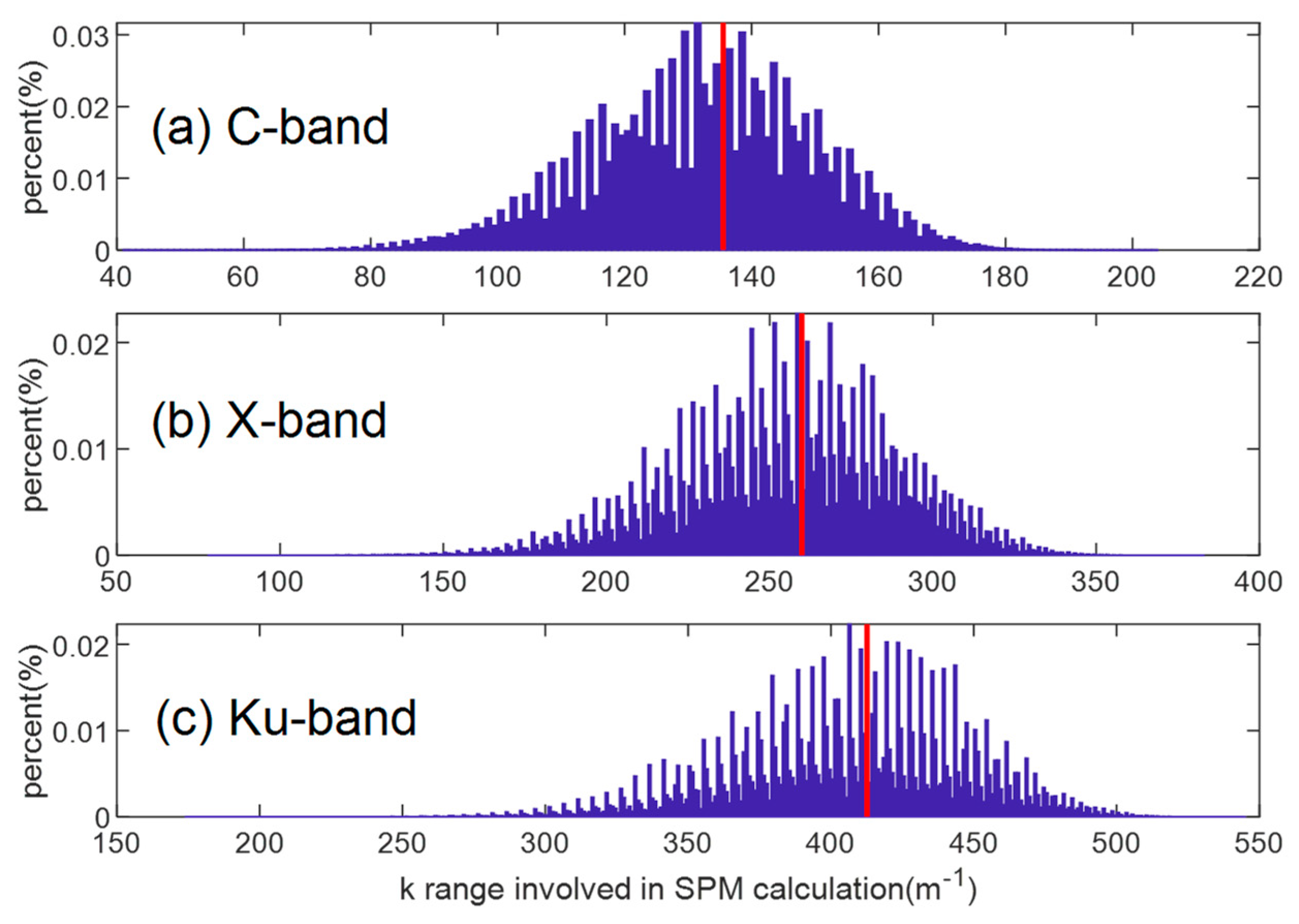
From these figures, we can also see that the simulation results of other models (dashed lines) are basically coincident, except for Johnson's model. To explain this phenomenon, Table 4 lists cutoff wavenumber values of different models and it shows that the cutoff wavenumbers of these models are different at the same incident conditions. To illustrate the reason why the TSM simulation results of different cutoff wavenumbers changes greatly, we select the large-scale surface slopes satisfying

p (s_{x}, s_{y}) > e^{- 25}

and calculate the local incident angles

θ_{il}

used in the integral term of Equation (7). Here, we assumed that the slope distributions of large-scale surface at different cutoff wavenumbers are basically the same due to slow changes of

s_{u}

s_{c}

with cutoff wavenumbers [24]. Then

2 k \sin θ_{il}

is used to get the wavenumber range involved in SPM calculation when the wave spectrum is not truncated.

Figure 15 shows the range and distribution of wavenumbers used in SPM before sea spectrum is divided, and the red line is the Bragg wavenumbers at the corresponding global incident conditions. In the final TSM simulation, only the components larger than the cutoff wavenumber are retained. The cutoff wavenumbers of other models in Table 4 seem ineffective for dividing the sea spectrum components in Figure 15. For example, the cutoff wavenumbers of Johnson's model are too large in these bands, so that the spectral components involved in SPM simulation are not included and the results are dominated by KA-GO. While the cutoff wavenumbers of other models are too small, and all spectrum components in Figure 15 are used for small-scale SPM. So, the simulated backscattering coefficients are all too large, as shown by the blue, red and black dashed lines in the Figure 12(a), 13(a), 14(a) and 14 (b). And it is also the reason that the simulation results of the fixed cutoff wavenumber, Guissard criterion and Li’s model are always basically the same in these three bands. In these cases, the division of sea spectrum becomes meaningless. The cutoff wavenumber of our model can effectively divide the sea spectrum into large and small scales, and the Bragg wavenumbers can contribute to the SPM computation. Table 4 also illustrates that other four models generally give a constant value for a given frequency as these models do not vary with the azimuth angle of satellite observation, while our model gives a value range. The comparison between the results of other cutoff wavenumber models and our empirical model in Figure 12(b) and Figure 13(b) suggests that different cutoff wavenumber should be valued for different incident azimuth angle.

Table 4. Cutoff wavenumbers of different models. The incident conditions in C-, X- and Ku-bands are consistent with those in Figure 12, Figure 13, Figure 14 and Figure 15.

	Cutoff wavenumber (C-band)	Cutoff wavenumber (X-band)	Cutoff wavenumber (Ku-band)
Fixed value	$k / 3 \approx 36.69$	$k / 3 \approx 67.37$	$k / 3 \approx 92.54$
Guissard et al.	32.55	62.42	89.58
Dongfang Li et al.	64.15	64.15	64.15
Johnson et al.	240.93	430.10	573.16
Optimal kc	105~136(vv) 67~115(hh)	214~253(vv) 151~196(hh)	405~448(vv) 275~341(hh)

5. Conclusions

The selection of the sea surface roughness spectrum and cutoff wavenumber is always important in the simulation analysis of sea surface EM scattering by TSM. By comparing the results of DV spectrum, Apel spectrum and Elfouhaily spectrum with their respective optimal cutoff wavenumbers, we concluded that Apel spectrum is more suitable for C-, X- and Ku-bands backscattering simulation of TSM. The optimal cutoff wavenumbers for different incident condition were numerically obtained by comparison the simulation results with the GMFs. Then, a four-variable polynomial containing twenty-six terms was obtained by regression analysis to represent these optimal cutoff wavenumbers. When the wind speed is 10m/s, the error between the simulation results using Apel spectrum and empirical function of cutoff wavenumber and the results of GMFs is less than 1dB. Compared with the simulation results of other cutoff wavenumber models, our cutoff wavenumber empirical function is obviously better. Besides, we also compared the performance of five classical seawater dielectric constant models based on the seawater dielectric constant data measured by Zhou et al. (2021), and finally chose GW2020 model proposed by Zhou et al. as the permittivity input of the two-scale model.

The conclusions obtained in this paper are applicable to the backscattering simulation of TSM with wind speed of 3~20m/s and incident angle of 30° ~ 66°. The lower limit was chosen based on the observation that when the incident angle is less than 30°, the minimum error between the simulation results of Apel spectrum and GMF mostly falls between 2~3dB. We analyzed the reason may be that KA-GO plays a dominant role in TSM when the incident angle is less than 30° as the KA-GO simulation results depend weakly on the selected cutoff wavenumber [24]. Hence, for small incident angle scattering, we plan to conduct an in-depth investigation into the Kirchhoff approximation and physical optics method (KA-PO) as a potential replacement for KA-GO in the future. What’s more, further research will be made on the EM scattering model of sea surface at wind speed above 20m/s and other frequency bands combining the satellite observation data and other more accurate sea surface geometric models.

Author Contributions

Conceptualization and methodology, Hongxia Ye; validation and writing, Chenyu Guo; supervision, Hongxia Ye. All authors have read and agreed to the published version of the manuscript.

Funding

This research was funded by the National Key Research & Development Program of China, No.2021YFB3900401.

Data Availability Statement

The XMOD2 model can be found here [1]. The HY-2 satellite data is available on line: https://osdds.nsoas.org.cn/.

Acknowledgments

The authors would like to thank the anonymous associate editor and reviewers for their persistent efforts in reading the manuscripts and for offering invaluable comments and suggestions that substantially improves this paper. The authors would like to thank Royal Netherlands Meteorological Institute scatterometer team for providing the codes of NSCAT-4 and CMOD7 GMFs, which are available on line: http://projects.knmi.nl/scatterometer/.

Conflicts of Interest

The authors declare no conflict of interest. The funders had no role in the design of the study; in the collection, analyses, or interpretation of data; in the writing of the manuscript; or in the decision to publish the results.

Appendix A. DV Spectrum

Durden and Vesecky proposed a new spectrum model based on the PM spectrum in 1985 to accurately described the spectral components behind the spectral peak of PM spectrum. The coefficients in the expression of DV spectrum were obtained by fitting RADSCAT 13.9GHz data with the two-scale method. The expression of DV spectrum is described as [18]

S (k_{ρ}) = \frac{0.004}{k_{ρ}^{3}} \times \{\begin{cases} \exp (0.74 g^{2} (\frac{1}{4 u_{19.5}^{4}} - \frac{1}{k_{ρ}^{2} u_{19.5}^{4}})) (k_{ρ} < 2) \\ {(\frac{1.25 k_{ρ} u_{*}^{2}}{g + 7.25 \times 10^{- 5} k_{ρ}^{2}})}^{0.225 \log (k_{ρ} / 2)} (k_{ρ} \geq 2) \end{cases},

(A1)

where

g = 9.81 m / s^{2}

u_{19.5}

is the wind speed at 19.5m above sea level,

u_{*}

is the friction velocity. Durden and Vesecky followed the spreading function of Fung and Lee as

ϕ (k_{ρ}, φ) = \frac{1}{2 π} [1 + \frac{2 \cos 2 φ (1 - R)}{(1 + R) (1 - D)} (1 - e^{- 0.00015 k_{ρ}^{2}})],

(A2)

R = \frac{3 + 1.92 u_{12.5}}{3.16 u_{12.5}},

(A3)

D = \frac{\int_{0}^{\infty} k_{ρ}^{2} S (k_{ρ}) e^{- 0.00015 k_{ρ}^{2}} d k_{ρ}}{\int_{0}^{\infty} k_{ρ}^{2} S (k_{ρ}) d k_{ρ}},

(A4)

Here

u_{12.5}

is the wind speed at 12.5m above sea level. The wind speed at any height

z

can be calculated as

u (z) = \frac{u_{*}}{0.4} \ln (\frac{z}{\frac{0.0000684}{u_{*}} + 0.00428 {u *}^{2} - 0.000443}),

(A5)

Appendix B. Apel Spectrum

In order to better interpret the radar images of ocean surfaces, Apel (1994) developed an improved spectrum model [19]. The omnidirectional spectrum followed the basic form of Banner spectrum, and he selected the second peak of the curvature spectrum (

B (k_{ρ}) = k_{ρ}^{3} S (k_{ρ})

) at 750 rad/m to conform with the measurement results. The omnidirectional spectrum is expressed as

S (k_{ρ}) = 0.0123 \frac{\exp (- k_{p}^{2} k_{ρ}^{- 2})}{k_{ρ}^{3}} {1.7}^{\exp [- \frac{{(k_{ρ}^{0.5} - k_{p}^{0.5})}^{2}}{0.32 k_{p}}]} H_{i},

(B1)

here

k_{p} = \frac{g}{\sqrt{2} u_{10}^{2}}

is the location of spectral peak,

u_{10}

is the wind speed at 10m above sea level.

H_{i}

is used to describe gravity capillary wave properties, and the expression is

H_{i} = [\frac{10000}{10000 + k_{ρ}^{2}} + 0.8 k_{ρ} \times 10^{- 4.95 + 3.45 (1 - \exp (- \frac{u_{10}}{4.7}))} \times sech (\frac{k_{ρ} - 400}{450})] \times e^{- {(\frac{k_{ρ}}{6283})}^{2}},

(B2)

The spreading function is improved based on the angular distribution function of Donelan and Banner, and is expressed as

ϕ (k_{ρ}, φ) = \frac{1}{2 π} \exp [- (0.14 + \frac{5 k_{p}^{1.3}}{k_{ρ}^{1.3}}) φ^{2}] .

(B3)

Appendix C. Elfouhaily Spectrum

Elfouhaily spectrum is a full-wave spectrum consisting of low-frequency gravitational wave spectrum and high-frequency tension wave spectrum, and is expressed as [16]

S (k_{ρ}) = \frac{1}{k_{ρ}^{3}} [F_{p} \frac{α_{p} c (k_{p})}{2 c (k_{ρ})} + F_{m} \frac{α_{m} c (k_{m})}{200 c (k_{ρ})}],

(C1)

α_{m} = \{\begin{cases} 1 + \ln (u_{*}) - \ln (0.23) u_{*} \leq 0.23 \\ 1 + 3 [\ln (u_{*}) - \ln (0.23)] u_{*} > 0.23 \end{cases},

(C2)

c (k_{ρ}) = \sqrt{\frac{g}{k_{ρ}} + \frac{g k_{ρ}}{k_{m}^{2}}},

(C3)

Here

k_{m} = 363 r a d / m

k_{p} = g \frac{Ω^{2}}{u_{10}^{2}}

α_{p} = 0.006 \sqrt{Ω}

(

Ω

is the wave age).

F_{p}

and

F_{m}

represent the side effect function of long and short waves respectively, and are expressed as

F_{p} = \exp [- \frac{1.25 k_{p}^{2}}{k_{ρ}^{2}} + \frac{Ω}{\sqrt{10}} (1 - \sqrt{\frac{k_{ρ}}{k_{p}}})] \cdot γ^{Γ},

(C4)

F_{m} = \exp [- \frac{1.25 k_{p}^{2}}{k_{ρ}^{2}} - {(\frac{k_{ρ} - k_{m}}{2 k_{m}})}^{2}] \cdot γ^{Γ},

(C5)

γ = \{\begin{cases} 1.7, 0.84 \leq Ω < 1 \\ 1.7 + 6 \log (Ω), 1 \leq Ω < 5 \\ 2.7 Ω^{0.57}, Ω \geq 5 \end{cases},

(C6)

Γ = \{\begin{cases} \exp [- 0.5 {((\sqrt{\frac{k_{ρ}}{k_{p}}} - 1) / (0.08 + 0.32 Ω^{- 3}))}^{2}], 0.84 \leq Ω < 5 \\ \exp [- 0.5 {((\sqrt{\frac{k_{ρ}}{k_{p}}} - 1) / 0.16)}^{2}], Ω \geq 5 \end{cases} .

(C7)

Elfouhaily proposed a unified directional transfer function based on the first two even-order harmonics of the Fourier series expansion. The expression is

ϕ (k_{ρ}, φ) = \frac{1}{2 π} [1 + Δ (k_{ρ}) \cos (2 φ)],

(C8)

Δ (k_{ρ}) = \tanh [\frac{\ln 2}{4} + \frac{4 c^{2.5} (k_{ρ})}{c^{2.5} (k_{p})} + \frac{0.13 u_{*} \cdot c^{1.5} (k_{m})}{c^{2.5} (k_{ρ})}]

(C9)

References

Li, X.-M.; Lehner, S. Algorithm for Sea Surface Wind Retrieval From TerraSAR-X and TanDEM-X Data. IEEE Trans. Geosci. Remote Sensing 2014, 52, 2928–2939. [Google Scholar] [CrossRef]
Sun, D.; Zhang, Y.; Wang, Y.; Chen, G.; Sun, H.; Yang, L.; Bai, Y.; Yu, F.; Zhao, C. Ocean Wave Inversion Based on Airborne IRA Images. IEEE Trans. Geosci. Remote Sensing 2022, 60, 1–13. [Google Scholar] [CrossRef]
Peng, Y.; Xie, X.; Lin, M.; Pan, C.; Li, H. A Modeling Study of the Impact of the Sea Surface Temperature on the Backscattering Coefficient and Wind Field Retrieval. IEEE Access 2020, 8, 78652–78662. [Google Scholar] [CrossRef]
Liu, Q.; Weng, F.; English, S.J. An Improved Fast Microwave Water Emissivity Model. IEEE Trans. Geosci. Remote Sensing 2011, 49, 1238–1250. [Google Scholar] [CrossRef]
Xie, D.; Chen, K.-S.; Yang, X. Effects of Wind Wave Spectra on Radar Backscatter From Sea Surface at Different Microwave Bands: A Numerical Study. IEEE Trans. Geosci. Remote Sensing 2019, 57, 6325–6334. [Google Scholar] [CrossRef]
Ryabkova, M.; Karaev, V.; Guo, J.; Titchenko, Yu. A Review of Wave Spectrum Models as Applied to the Problem of Radar Probing of the Sea Surface. JGR Oceans 2019, 124, 7104–7134. [Google Scholar] [CrossRef]
Yueh, S.H. Modeling of Wind Direction Signals in Polarimetric Sea Surface Brightness Temperatures. IEEE Trans. Geosci. Remote Sensing 1997, 35, 1400–1418. [Google Scholar] [CrossRef]
Wang, T.; Tong, C. An Improved Facet-Based TSM for Electromagnetic Scattering From Ocean Surface. IEEE Geosci. Remote Sensing Lett. 2018, 15, 644–648. [Google Scholar] [CrossRef]
Meissner, T.; Wentz, F.J. The Complex Dielectric Constant of Pure and Sea Water from Microwave Satellite Observations. IEEE Trans. Geosci. Remote Sensing 2004, 42, 1836–1849. [Google Scholar] [CrossRef]
Meissner, T.; Wentz, F.J.; Ricciardulli, L. The Emission and Scattering of L-band Microwave Radiation from Rough Ocean Surfaces and Wind Speed Measurements from the Aquarius Sensor. JGR Oceans 2014, 119, 6499–6522. [Google Scholar] [CrossRef]
Zhou, Y.; Lang, R.H.; Dinnat, E.P.; Le Vine, D.M. Seawater Debye Model Function at L-Band and Its Impact on Salinity Retrieval From Aquarius Satellite Data. IEEE Trans. Geosci. Remote Sensing 2021, 59, 8103–8116. [Google Scholar] [CrossRef]
Thermal Microwave Radiation: Applications for Remote Sensing; Mätzler, C., Institution of Engineering and Technology, Eds.; IET electromagnetic waves series; Institution of Engineering and Technology: London, 2006; ISBN 9780863415739.
Pierson, W.J.; Moskowitz, L. A Proposed Spectral Form for Fully Developed Wind Seas Based on the Similarity Theory of S. A. Kitaigorodskii. J. Geophys. Res. 1964, 69, 5181–5190. [Google Scholar] [CrossRef]
Preisendorfer, R.W.; Mobley, C.D. Albedos and Glitter Patterns of a Wind-Roughened Sea Surface. J. Phys. Oceanogr. 1986, 16, 1293–1316. [Google Scholar] [CrossRef]
Kudryavtsev, V.; Hauser, D.; Caudal, G.; Chapron, B. A Semiempirical Model of the Normalized Radar Cross-section of the Sea Surface 1. Background Model. J. Geophys. Res. 2003, 108. [Google Scholar] [CrossRef]
Elfouhaily, T.; Chapron, B.; Katsaros, K.; Vandemark, D. A Unified Directional Spectrum for Long and Short Wind-driven Waves. J. Geophys. Res. 1997, 102, 15781–15796. [Google Scholar] [CrossRef]
Hwang, P.A.; Fois, F. Surface Roughness and Breaking Wave Properties Retrieved from Polarimetric Microwave Radar Backscattering. JGR Oceans 2015, 120, 3640–3657. [Google Scholar] [CrossRef]
Durden, S.; Vesecky, J. A Physical Radar Cross-Section Model for a Wind-Driven Sea with Swell. IEEE J. Oceanic Eng. 1985, 10, 445–451. [Google Scholar] [CrossRef]
Apel, J.R. An Improved Model of the Ocean Surface Wave Vector Spectrum and Its Effects on Radar Backscatter. J. Geophys. Res. 1994, 99, 16269–16291. [Google Scholar] [CrossRef]
Wentz, F.J. A Two-Scale Scattering Model for Foam-Free Sea Microwave Brightness Temperatures. J. Geophys. Res. 1975, 80, 3441–3446. [Google Scholar] [CrossRef]
Plant, W.J. A Two-scale Model of Short Wind-generated Waves and Scatterometry. J. Geophys. Res. 1986, 91, 10735–10749. [Google Scholar] [CrossRef]
Guissard, A.; Sobieski, P. An Approximate Model for the Microwave Brightness Temperature of the Sea. International Journal of Remote Sensing 1987, 8, 1607–1627. [Google Scholar] [CrossRef]
Li, D.; Zhao, Z.; Qi, C.; Huang, Y.; Zhao, Y.; Nie, Z. An Improved Two-Scale Model for Electromagnetic Backscattering From Sea Surface. IEEE Geosci. Remote Sensing Lett. 2020, 17, 953–957. [Google Scholar] [CrossRef]
Johnson, J.T.; Raines, E.; Toporkov, J.V.; Hwang, P.; Ouellette, J.D. On the Cutoff Wavenumber in the Geometrical Optics Theory of Near Specular Scattering from the Sea Surface. In Proceedings of the IGARSS 2022 - 2022 IEEE International Geoscience and Remote Sensing Symposium; IEEE: Kuala Lumpur, Malaysia, July 17 2022; pp. 4963–4965.
Stoffelen, A.; Verspeek, J.A.; Vogelzang, J.; Verhoef, A. The CMOD7 Geophysical Model Function for ASCAT and ERS Wind Retrievals. IEEE J. Sel. Top. Appl. Earth Observations Remote Sensing 2017, 10, 2123–2134. [Google Scholar] [CrossRef]
Royal Netherlands Meteorological Institute. NSCAT-4 Geophysical Model Function, Accessed: Mar. 1, 2016. Available online: http://projects.knmi.nl/scatterometer/nscat_gmf/.
Tsang, L.; Kong, J.A. Scattering of Electromagnetic Waves: Advanced Topics; 1st ed.; Wiley, 2001; ISBN 9780471388012.
Quegan, S. Understanding Synthetic Aperture Radar Images; Oliver, C. (Eds.) ; The SciTech radar und defense series; SciTech Publishing, Inc: Raleigh, NC, 2004; ISBN 9781891121319. [Google Scholar]
Shao, W.; Zhang, Z.; Li, X.; Wang, W. Sea Surface Wind Speed Retrieval From TerraSAR-X HH Polarization Data Using an Improved Polarization Ratio Model. IEEE J. Sel. Top. Appl. Earth Observations Remote Sensing 2016, 9, 4991–4997. [Google Scholar] [CrossRef]
Bishop, C.M. Pattern Recognition and Machine Learning; Information science and statistics; Springer: New York, 2006; ISBN 9780387310732. [Google Scholar]
Scikit-learn: Machine Learning in Python, Pedregosa et al., JMLR 12, pp. 2825-2830, 2011.

Figure 2. Comparison of real and imaginary parts of four permittivity models with data.

Figure 3. Comparison of different sea spectrums.

Figure 4. The error between the TSM simulation (DV spectrum) and the NSCAT-4 model when taking different cutoff wavenumbers. (a) The error variation of different wind speeds at 10m (

θ_{i} = 20 °

φ_{i} = 0 °

); (b) The error variation of different incident angles (

φ_{i} = 90 °

u_{10} = 5 m / s

Figure 4. The error between the TSM simulation (DV spectrum) and the NSCAT-4 model when taking different cutoff wavenumbers. (a) The error variation of different wind speeds at 10m (

θ_{i} = 20 °

φ_{i} = 0 °

); (b) The error variation of different incident angles (

φ_{i} = 90 °

u_{10} = 5 m / s

Figure 5. Variation of cutoff wavenumber with wind speed given by different models.

Figure 6. Minimum absolute error of three spectrums at C-, X- and Ku-bands. (

θ_{i} = 30 °

φ_{i} = 90 °

Figure 6. Minimum absolute error of three spectrums at C-, X- and Ku-bands. (

θ_{i} = 30 °

φ_{i} = 90 °

Figure 7. The optimal cutoff wavenumber vs. incident angle and azimuth angle (

u_{10}

= 5 m/s,

f

= 13.256 GHz). The gray surface represents the Bragg wavenumber.

Figure 7. The optimal cutoff wavenumber vs. incident angle and azimuth angle (

u_{10}

= 5 m/s,

f

= 13.256 GHz). The gray surface represents the Bragg wavenumber.

Figure 8. Evaluate the fitting results using n-order polynomial. The data used for fitting correspond to the optimal cutoff wavenumber values for the Apel spectrum in C-, X-, and Ku-bands under vertical polarization.

Figure 9. Evaluate the fitting results using n-order polynomial. The data used for fitting correspond to the optimal cutoff wavenumber values for the Apel spectrum in Ku-band under horizontal polarization.

Figure 15. The range and distribution of sea wavenumbers involved in SPM calculation. (a) C-band,

θ_{i} = 38 °

u_{10} = 10

m/s; (b) X-band,

θ_{i} = 40 °

u_{10} = 10

m/s; (c) Ku-band,

θ_{i} = 48.5 °

u_{10} = 10

m/s. The red lines in (a), (b) and (c) are Bragg wavenumbers of the corresponding incident angles.

Figure 15. The range and distribution of sea wavenumbers involved in SPM calculation. (a) C-band,

θ_{i} = 38 °

u_{10} = 10

m/s; (b) X-band,

θ_{i} = 40 °

u_{10} = 10

m/s; (c) Ku-band,

θ_{i} = 48.5 °

u_{10} = 10

m/s. The red lines in (a), (b) and (c) are Bragg wavenumbers of the corresponding incident angles.

Table 1. The Incident angle range of GMFs in different bands.

Frequency Band	Incident Angle Range
C-band	$30 ° ~ 66 °$
X-band	$30 ° ~ 45 °$
Ku-band	$30 ° ~ 66 °$

Disclaimer/Publisher’s Note: The statements, opinions and data contained in all publications are solely those of the individual author(s) and contributor(s) and not of MDPI and/or the editor(s). MDPI and/or the editor(s) disclaim responsibility for any injury to people or property resulting from any ideas, methods, instructions or products referred to in the content.

© 2023 by the authors. Licensee MDPI, Basel, Switzerland. This article is an open access article distributed under the terms and conditions of the Creative Commons Attribution (CC BY) license (http://creativecommons.org/licenses/by/4.0/).

Copyright: This open access article is published under a Creative Commons CC BY 4.0 license, which permit the free download, distribution, and reuse, provided that the author and preprint are cited in any reuse.

MDPI Initiatives

Important Links

Choose an area of interest and we will send you notifications of new preprints at your preferred frequency.

Disclaimer

Quantitative Research of Cutoff Wavenumber and Wave Spectrum for Electromagnetic Scattering Computation with Two-Scale Method

Abstract

1. Introduction

2. The Theory of Two-Scale Method

3. Key factors of TSM Model

3.1. Permittivity model of Seawater

3.2. Spectrum Model of Rough Sea Surface

3.3. Effect of Different Cutoff Wavenumbers

3.4. The Selection of Spectrum and Cutoff Wavenumber

3.5. Empirical Function of Optimal Cutoff Wavenumber

4. Comparison and Discussion

5. Conclusions

Author Contributions

Funding

Data Availability Statement

Acknowledgments

Conflicts of Interest

Appendix A. DV Spectrum

Appendix B. Apel Spectrum

Appendix C. Elfouhaily Spectrum

References

MDPI Initiatives

Important Links

Subscribe