1. Introduction
Marine plankton species diversity governs one of the most important ecosystem functions - biological productivity [
1]. Phytoplankton are responsible for the annual production of approximately 50% of the Earth's net primary production [
2]. It is mainly consumed by zooplankton which in turn supports planktivorous fish production. Together with the structure of the ecosystem, which contains its biotic and abiotic elements, these functions generate an essential service – the habitat [
3] which, if healthy, creates important social and economic benefits for the coastal community. Romania’s "Blue Economy" sector is undeveloped, both in comparison with other European Union (EU) member states and with other national economic sectors. With just over one billion euros, it represented, in 2018, 0.6% of the national economy and 66,600 jobs [
4]. Of these, the living resources sector generated only 85 million euros and 6,200 jobs. Excluding issues related to legislative gaps and organizational shortcomings (such as the absence of a maritime spatial plan and the failure to designate areas for aquaculture), it can be said that the growth prospects rely on the well-being of the ecosystem. The health of the ecosystem depends mainly on the intensity of the pressures to which it is subjected. The northwestern area of the Black Sea has endured, over time, several abrupt changes in the transition from a low-production system (the 1970s) to a highly eutrophicated system (1980s) and then an intermediate state with relatively low biomass (90s-00s), when bacterioplankton, zooplankton and living marine resources had low quantities. Still, the nonfodder component of zooplankton (
Noctiluca scintillans), and gelatinous organisms were at moderate levels, indicating a degraded ecosystem [
5] and not a trend of improvement and rehabilitation [
6]. All these regimes were mainly driven by nutrient discharges from point and diffuse sources. Nowadays, to these are added the effects of climate change, by warming the seawater, which is expected to cause the extinction of some species in the future by exceeding their thermal limit and the restructuring of the community’s composition, both associated with possible consequences on the functioning of the marine food chain and biogeochemical cycles [
1].
Unfortunately, current managerial practices are considered ineffective in managing complex phenomena, such as ecosystem regime changes, due to the lack of adequate explanatory models [
7]. Thus, the use of semi-quantitative modelling coupled with statistical methods (Machine Learning) to assess the natural and anthropogenic variability of the relationships between abiotic factors and different trophic levels of the marine ecosystem can facilitate the understanding of less known processes that may occur within the ecosystem.
This was achieved in this study through the application of semi-quantitative modelling (Mental Modeler – Fuzzy Cognitive Maps) and machine learning algorithms (Machine Learning) that create the model for generating applicable predictions in decision-making regarding the management of pressures on the marine ecosystem. Thus, for the success of decisions, the model can distinguish between factors by generating robust results and improving case study analysis methods [
8].
However, the purpose of the modelling is fully achieved if we run scenarios resulting from the combination of variables and their variability to predict the behaviour of the ecosystem.
The objective of the study is to introduce qualitative and semi-quantitative modelling coupled with machine learning algorithms to assess the natural variability and anthropogenic impact of the relationships between abiotic factors and the first two trophic levels of the marine ecosystem and run the scenarios to predict the behaviour of the ecosystem.
2. Materials and Methods
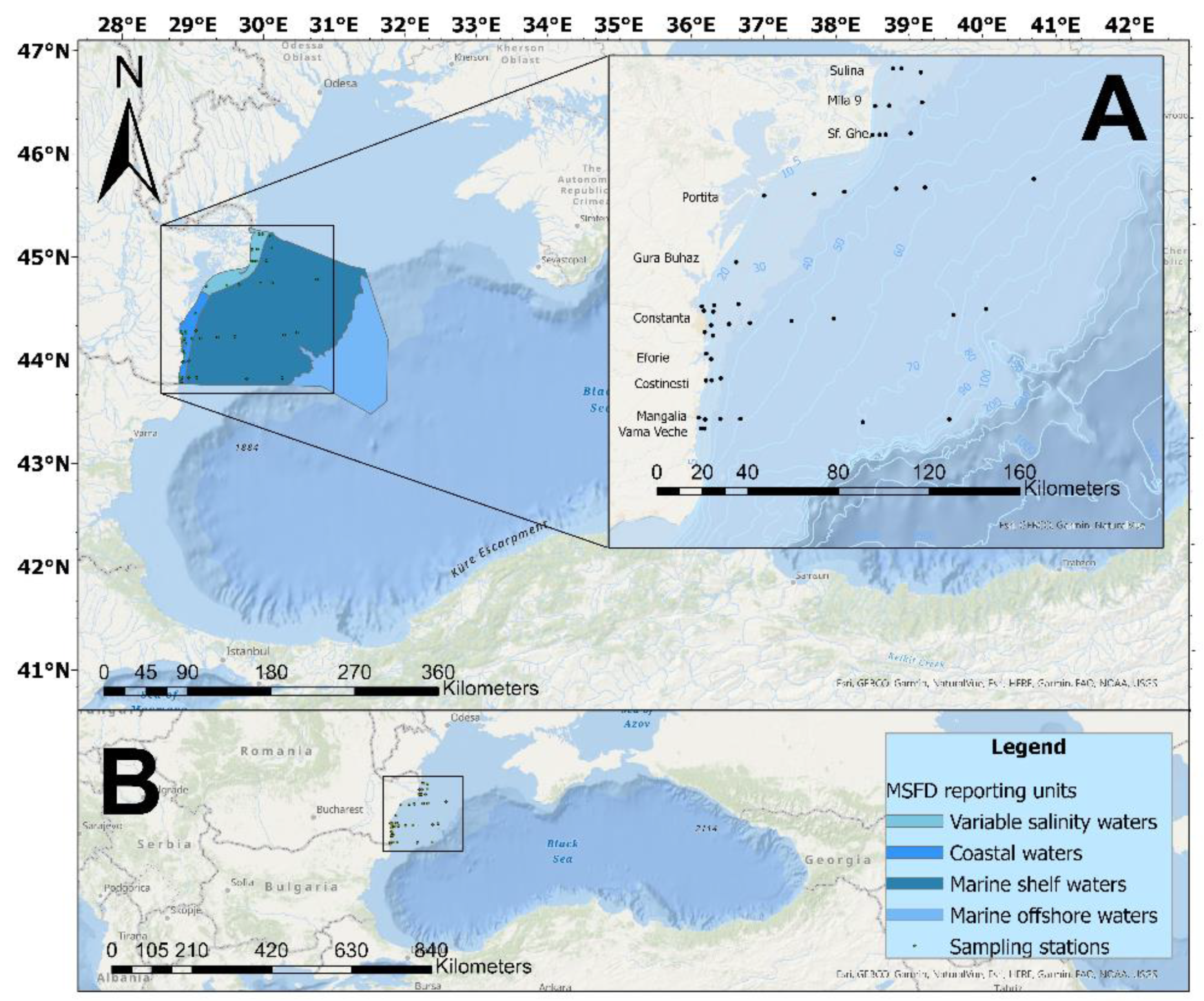
Seawater and biological (for phytoplankton and zooplankton) samples were collected in expeditions organized in the warm season (from May to September) of 2008-2018, on the Black Sea monitoring network consisting of 39 stations located in variable salinity, coastal and marine waters (
Figure 1). 2012 was not included in the analysis, as in this year expeditions were undertaken only in the cold season.
Phytoplankton and zooplankton samples were collected and analysed according to the methodology [
9,
10].
Temperature and salinity were measured using the reversible thermometer and the titration method, as well as the CastAway CTD multiparameter probe (YSI Cast Away model).
Dissolved nutrient concentrations were determined according to standard methods for seawater analysis [
11].
Data statistics and their visualization were performed with STATISTICA 14.0.0.15 [
12], an advanced software package that provides data analysis, data management, statistics, data mining, machine learning, text analysis and data visualization procedures. The data were analyzed by general descriptive statistics and visualized (boxplot) then the correlations between the parameters (Pearson coefficient, r) were performed which determine the extent to which the values of two variables are "proportional" to each other. The significance level (p) calculated for each correlation is a primary source of information about the reliability of the correlation. In the statistical analysis, the threshold value p=0.05 and a sufficient number of data (over 100) were used so that the hypothesis of normality was respected.
The semi-quantitative modelling was carried out with the Mental Modeler software - a decision support software (open-source,
https://www.mentalmodeler.com/) that helps experts understand the impact associated with environmental changes and develop strategies for reducing unwanted outcomes by capturing, communicating, and representing knowledge. By building Cognitive Knowledge Maps (FCMs), the Mental Modeler allows to development of the semi-quantitative model that: (1) defines the important components (2) defines the strength of the relationships between the components and (3) runs scenarios that determine how the system reacts in certain conditions [
13].
ArcGIS Desktop 10.7 software (ESRI, 2019) [
14] was used for creating distribution maps and machine learning (ML) algorithms. The basic premise of ML is that a machine (ie an algorithm or model) can make predictions based on existing data. The basic technique behind all ML methods is an iterative combination of statistics and error minimization, applied and combined to varying degrees. Many ML algorithms iteratively check all or a very large number of possible outcomes to find the best outcome for the problem at hand. The potentially large number of iterations is prohibitive for manual calculations and is a large part of the reason these methods are only now widely available to individual researchers.
1. The first step in applying ML was to learn the algorithm using the training dataset (2008-2018) which consists of the independent variables (abiotic components – T, S, PO4, DIN) with dependent variables (total phytoplankton density). The training data is used to "learn" how the independent (input) variables relate to the dependent (output) variable.
2. In step two, when the algorithm has applied to new input data, corresponding to the scenarios to be tested, the model applies the learned relationship and returns a prediction. After the algorithm is trained, it must be tested to obtain a measure of the quality of predictions from new data.
3. This requires another data set with independent and dependent variables, but the dependent (target) variables are not provided (10-20% of the original data). Algorithm predictions (output) are compared with retained data (target) to validate the algorithm. This comparison represents the significant difference between ML and traditional statistical techniques that use p-values for validation.
ArcGIS creates models and generates predictions using an adaptation of the random forest algorithm (Leo Breinman) called Forest-based Classification and Regression, a supervised machine learning method. Predictions can be made for both categorical (classification) and continuous (regression) variables. By default, ML uses 90% of the data to build the model and 10% to validate it.
Two scenarios for forecasting the growth of phytoplankton and zooplankton were developed and analysed: Bussiness as Usual in which temperature increases by 0.4 oC, salinity increases by 0.84‰ and nutrient levels remains constant and the Mild scenario, in which sea water temperature increases by 0.8 oC and salinity increases by 1.68‰ and nutrients concentrations are decreased by 25% for phosphates and 70% for inorganic nitrogen until 2042.
3. Results
3.1. Semi-quantitative model of causal relationships between abiotic factors (temperature, salinity and nutrients) and two trophic levels
The water temperature recorded values in the range of 13.5 - 28.0
oC, the variability - expressed as standard deviation being 3.51
oC. Over the entire analyzed period, an increasing trend was observed, with 0.18
oC, equivalent to an average of 0.02
oC/year. The salinity ranged from 0.11 to 20.00‰, with values lower than 6.06‰ being uncharacteristic (outliers). During the warm season, there is a noticeable upward trend in salinity variation, with an increase of 0.42‰ (
Table S1 and
Figure 2). This is primarily attributed to the significant influence of evaporation and the mixing of water masses, which surpasses the impact of river and precipitation input.
Against the backdrop of increasingly dry summers, a slight decrease in phosphates and silicates was also observed, nutrients whose external input is largely influenced by river input and continental drainage (
Figure 2) (r
po4-s = -0.37; r
sio4 -s = -0.72). The levels of inorganic nitrogen forms (nitrites, nitrates, ammonium) have different variations during the analyzed period. Thus, nitrites and nitrates have increasing trends by 0.08 µM and 0.20 µM, respectively, while ammonium decreases by 0.28 µM (
Figure 2).
In all cases, uncharacteristic values (outliers) and extremes of the concentrations of nutrients dissolved in seawater were also observed.
Within the phytoplankton assembly, a total of 298 species were distinguished, spanning diverse varieties and forms spread across 16 taxonomic classes (Bacillariophyceae, Chlorodendrophyceae, Chlorophyceae, Chrysophyceae, Conjugatophyceae, Cryptophyceae, Cyanophyceae, Dictyochophyceae, Dinophyceae, Ebriophyceae, Euglenoidea, Prasinophyceae, Prymnesiophyceae, Trebouxiophyceae, Ulvophyceae, and Xanthophyceae). The peak species count, 160 species, occurred in 2013, while the lowest count, 71 species, was recorded in 2016. Diatoms (102 species) and dinoflagellates (76 species) constituted the majority, contributing to 60% of the overall species diversity, followed by chlorophytes (46 species) and cyanobacteria (31 species) at 15% and 10%, respectively. In less diverse classes (comprising 5 to 14 species), the Trebouxiophyceae class contributed 5% to the total species count, while both Euglenoidea and Cryptophyceae represented 2% each. Classes exhibiting lower diversity (containing 1-4 species), including Chlorodendrophyceae, Conjugatophyceae, Chrysophyceae, Dictyochophyceae, Ebriophyceae, Prymnesiophyceae, Ulvophyceae, and Xanthophyceae, collectively constituted 6% of the qualitative composition (
Figure 3).The yearly means for overall phytoplankton density fluctuated between 245.33x10
3 cells/L (in 2016) and 4.10x10
6 cells/L (in 2014). Regarding biomass, the average annual values ranged from 370 mg/m
3 (in 2016) to 2820 mg/m
3 (in 2009) (
Table S1).
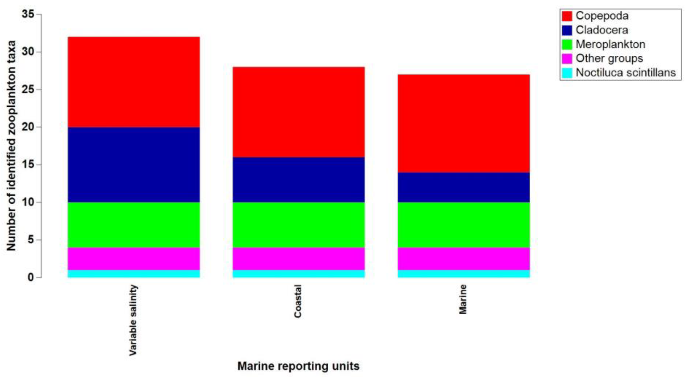
Between 2008 and 2018, a total of 32 zooplankton taxa were identified, with the highest count found in waters with variable salinity under the Danube's discharge influence. Copepods prevailed across all marine regions, followed by ten species of cladocerans in areas with variable salinity. The meroplanktonic group encompassed six taxa, while the "other groups" category included three species (
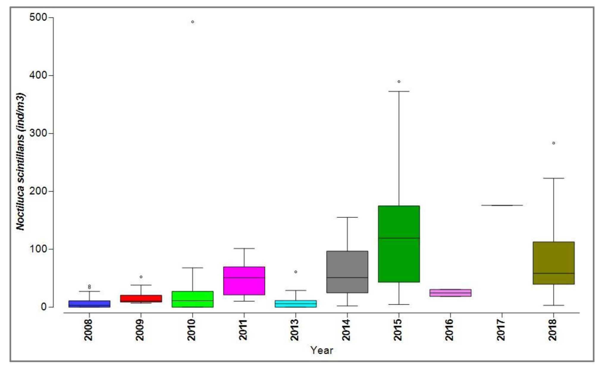
Figure 4). Along the entire Black Sea coast, the nonfodder component was evident, with the dinoflagellate N. scintillans being the sole representative species (
Figure 5). Fodder zooplankton exhibited fluctuations in both density and biomass, reaching a peak annual density of 51,430 ind/m
3 and a maximum annual biomass of 1,539 mg/m
3, both in 2018 (
Table S1).
N. scintillans exhibited notable quantitative fluctuations, particularly high biomass and density were observed in 2010, 2015, and 2018, marked by some atypical values (outliers) (
Figure 5).
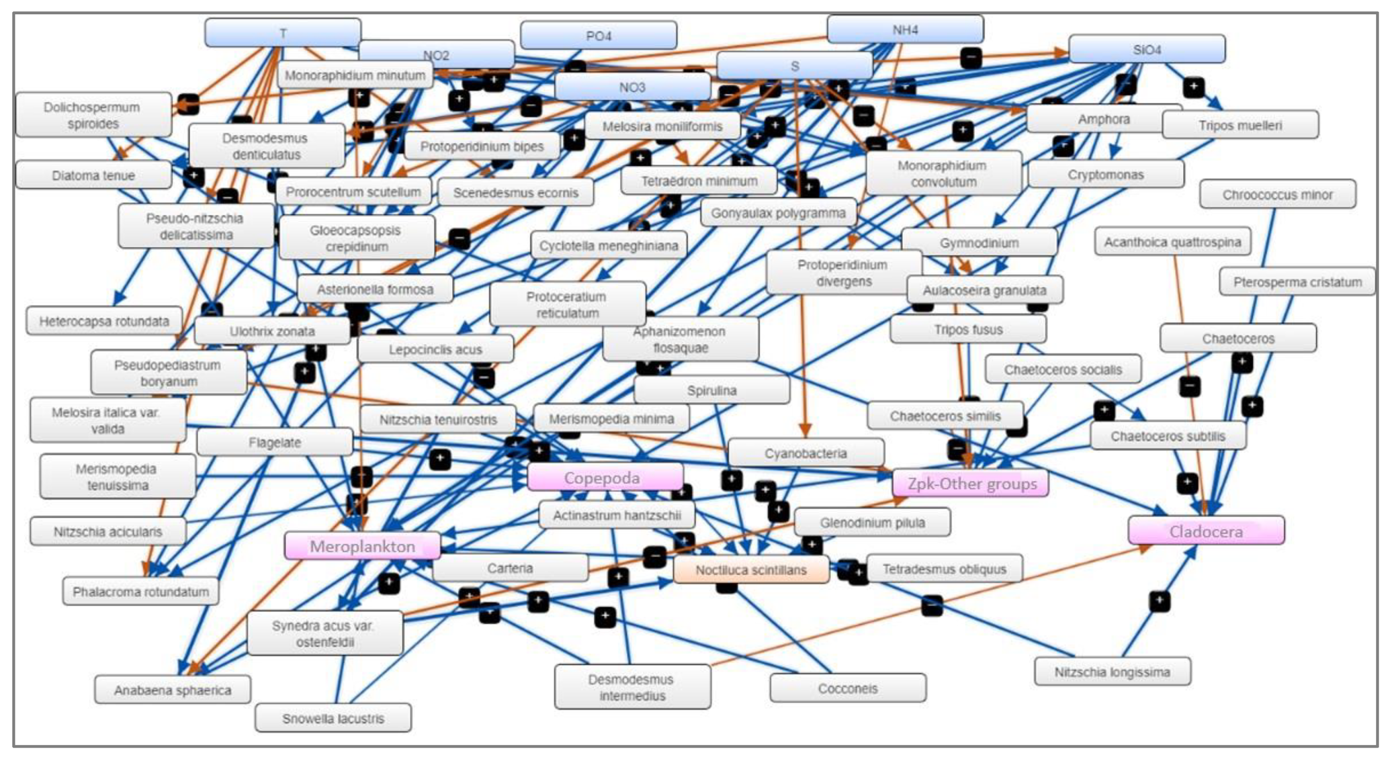
The analysis of significant correlations between the three levels of the marine ecosystem (abiotic components - temperature, salinity and nutrients; phytoplankton - species densities and zooplankton - group densities) led to the creation of the Mental Modeler model. Examining the noteworthy correlations among the abiotic and biotic components resulted in the development of the Mental Modeler model.
In this context, the aim of these "models" isn't to predict the state of this intricate ecosystem but rather to semi-quantitatively assess (using significant correlation coefficients) the connections among the various components. These connections serve as working hypotheses in the subsequent development of scenarios. Thus, FCM uses three characteristics of the studied system:
- System components (N=89) – abiotic parameters (T, S, nutrients), phytoplankton species with more than 10 presences, zooplankton groups,
- Positive or negative relationships between components (N=203) – significant correlations, greater than ±0.50, between components,
- The degree of influence that one component can have on another, defined by qualitative weights (for example, high, medium or low influence) - the significant correlations (p<0.05) coefficient between the system components.
Thus, apart from temperature as the main abiotic driver, the model identified as the main "drivers" (out of a total of 31), in order of importance, the concentrations of silicates and ammonium, and as "receivers" (out of a total of 26) the densities of “other groups” and copepods (
Figure 6).
3.2. Ecosystem evolution scenarios under climate change conditions from the Romanian coast of the Black Sea using FCM and ML
Models based on two data sets – normal phytoplankton (domain without outliers and extremes) development (N=7107) and phytoplankton blooms (over 1 million cel/L) were analysed (N=756), to which we applied two development scenarios aiming at predicting the density of copepods, cladocerans, meroplankton, other zooplankton groups and the density of N. scintillans. The explanatory variables used were temperature (oC), salinity (‰) and concentrations of phosphates (PO4) and inorganic nitrogen (DIN - the sum of nitrates, nitrites and ammonium) (µM) to which we added the total phytoplankton density (cel/L ) in the case of zooplankton predictions.
A separate model was developed for each prediction resulting in 12 regression models with different performances (
Table 1). One of the performance parameters of the model is the regression coefficient R
2 which represents the proportion of variation in the result that the model can predict based on its characteristics and which is easily calculated with formula (1).
With one exception, good results are observed when validating the models, expressed in the form of R2 regression coefficients. Therefore, given the poor performance (0.17) of the model described by the explanatory variables chosen for Total phytoplankton density - normal conditions, it will be excluded from the following discussions in applying the scenarios.
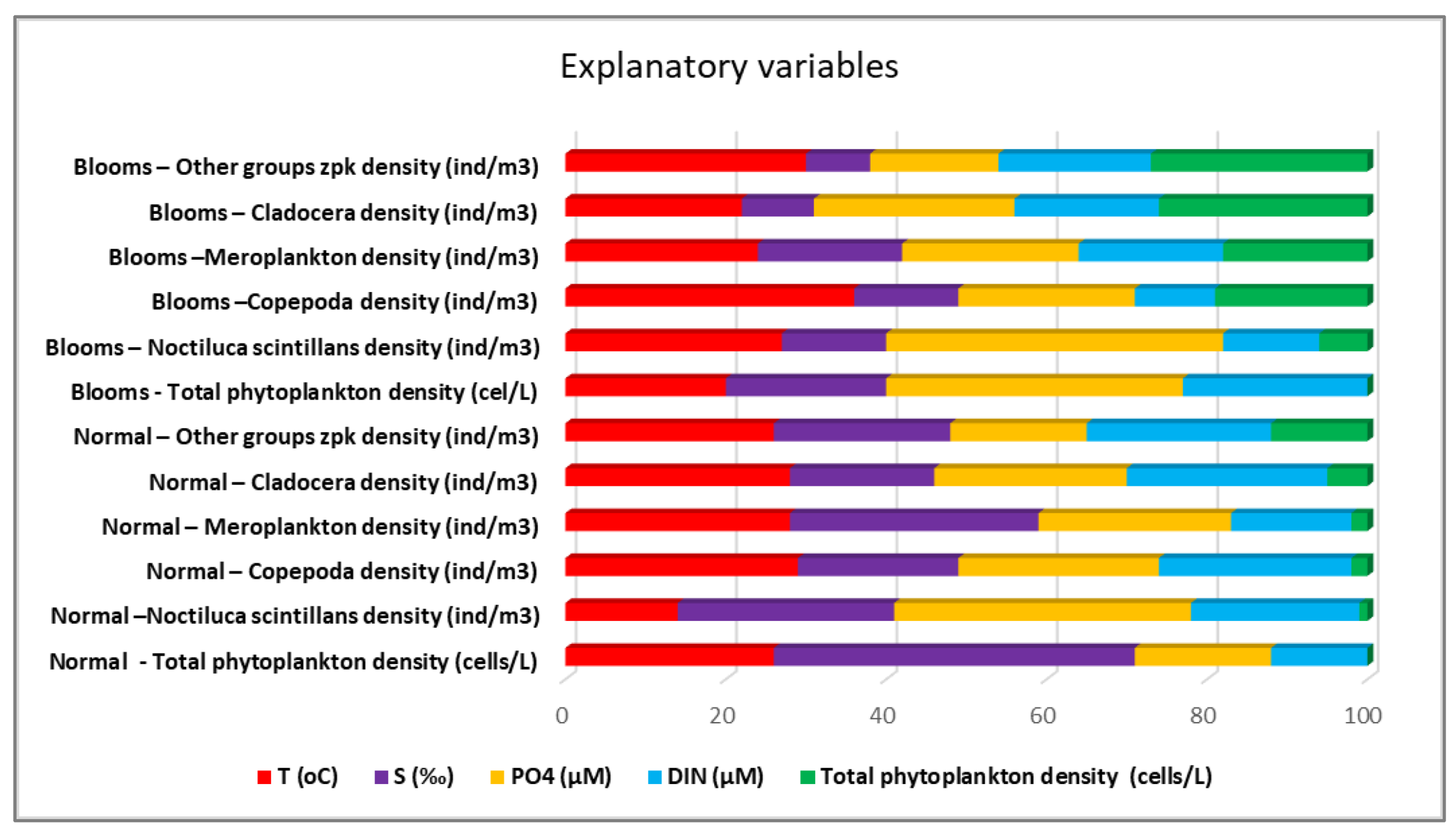
Although the collected data refer to a single season, the warm one, the importance of water temperature is observed, which is the dominant variable in the case of the density of copepods (36%) and “other” zooplankton groups (30%) during the blooming period. Water temperature had the least influence on
N. scintillans under normal conditions. Fluctuations in salinity, closely linked to variations in silicate levels—typically associated with riverine input—have a significant impact on the regular growth of phytoplankton. However, the proliferation of extensive phytoplankton blooms is primarily attributed to phosphate concentrations, which, notably, did not exhibit significant correlations with salinity throughout the study period. This suggests that the phosphate source responsible for these blooms may not be the result of riverine input (
Figure 7). It is well recognised that certain taxonomic groups of zooplankton have strong relationships with particular hydrographic, physical, and chemical circumstances, as well as with the phytoplankton composition [
15]. This most likely translates into particular characteristics or quantitative trait values that are more or less strongly correlated with particular physico-chemical circumstances and phytoplankton composition. Using fitness maximisation techniques, trait-based models may be able to forecast which strategies will be chosen in a given environment [
16]
.
Similar to previous research findings documented in Lomartire et al., [
17], it has been observed that the overall density of phytoplankton exerts a limited influence on the proliferation of non-fodder zooplankton, such as N. scintillans. However, it does facilitate the prevalence of "other groups" and cladocerans, especially evident during expansive bloom occurrences.
3.3. Working hypotheses for future research on planktonic proliferations in the Romanian area of the Black Sea
Taking into account the above, we developed and run two scenarios (which do not take into account the socio-economic development aspects of the area) to predict the development of the pelagic biological components (phytoplankton and zooplankton) in the warm season in the next 20 years (2042):
1. The BAU (Business As Usual) scenario in which the variables behave as they did during the study period – temperature increases by 0.4 oC, salinity increases by 0.84‰, and nutrient concentrations remain constant.
2. The scenario corresponding to RCP2.6, the "mildest" climate warming scenario in which sea water temperature increases by 0.8
oC by 2050 [
18]. Associated with this increase, we consider an increase in salinity by 1.68‰. Given that such a scenario envisages environmental protection measures and emission reduction, we consider that nutrient concentrations could also be reduced by 25% for phosphates and 70% for inorganic nitrogen [
19].
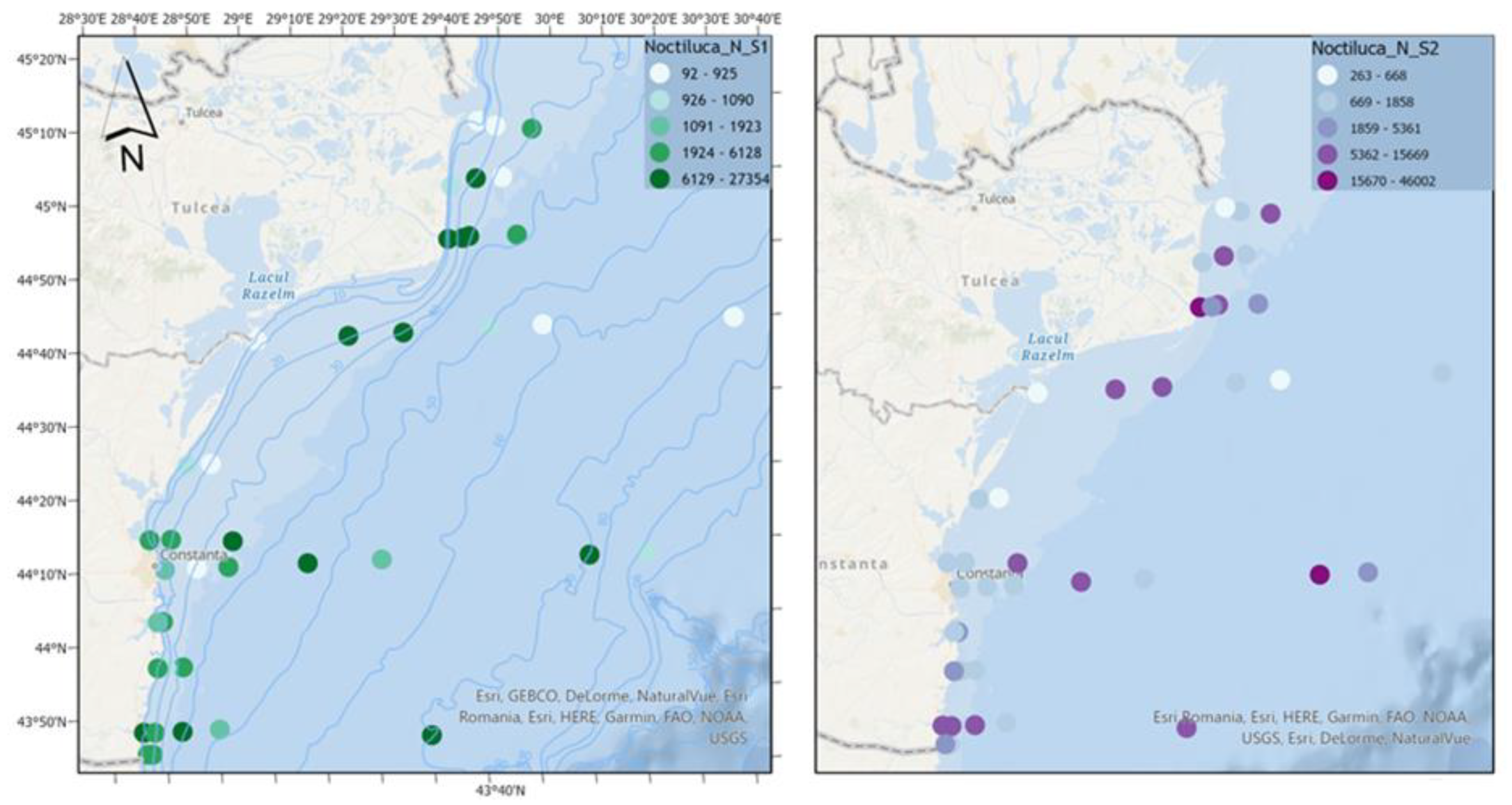
For the dinoflagellate N. scintillans, it is observed that in both scenarios high densities of the species are reached (with extreme values that in scenario 2 exceed scenario 1 by approximately 70%), characteristic of a eutrophic ecosystem (
Figure 8).
Spatial analysis indicates that in scenario 1, lacking nutrient reduction strategies, elevated abundances are observed in the coastal region. However, in scenario 2, marked by substantial nutrient reduction efforts amidst amplified climate change impacts, non-fodder zooplankton displays comparable abundance levels in the coastal area and heightened values offshore. This shift potentially introduces imbalances, underscoring the critical significance of reducing nutrients within the context of climate change scenarios.
Copepods, a major component of marine zooplankton, are the main food source of fish larvae [
20], favoring the survival, growth and development of juvenile fish [
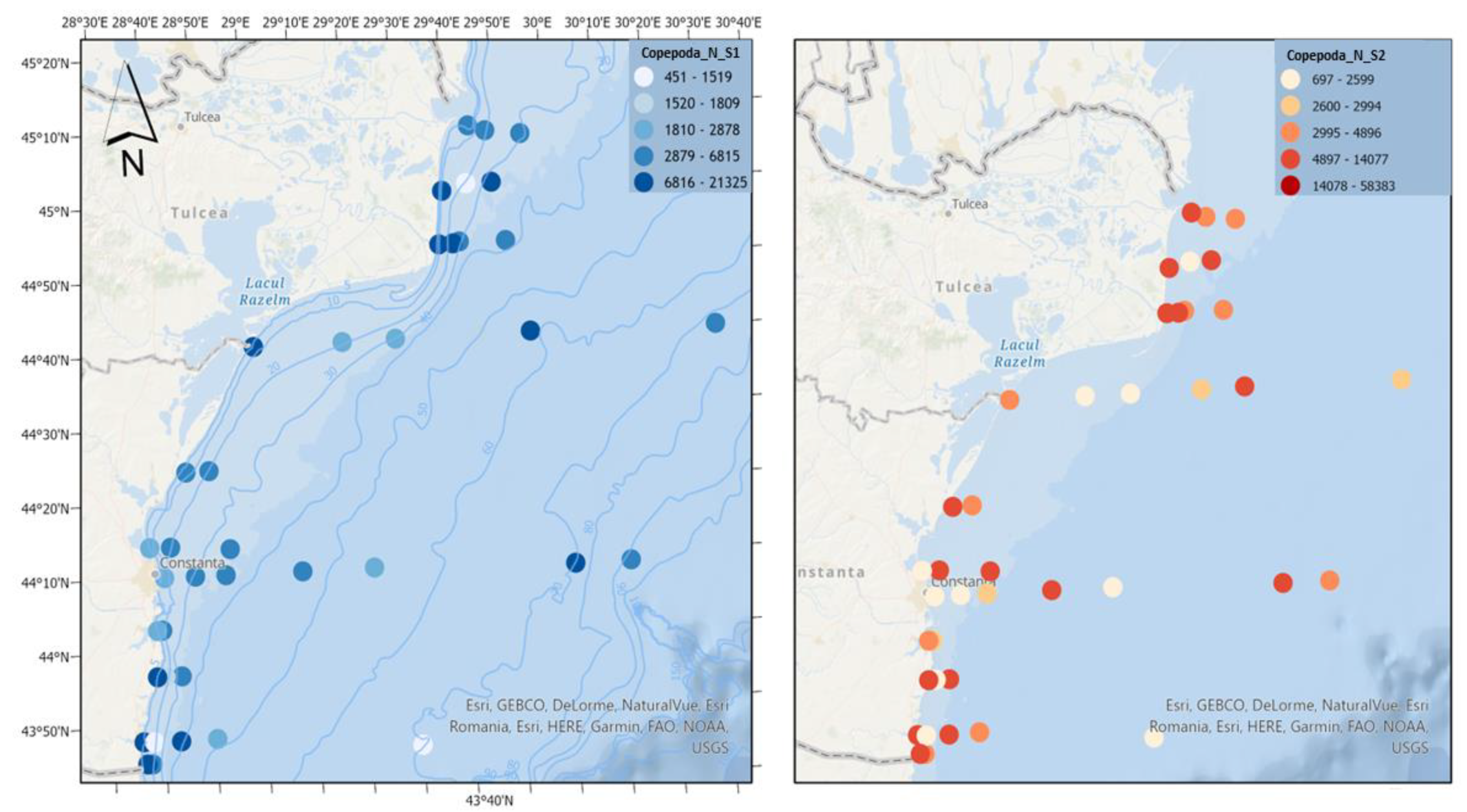
21]. It is observed that in the first scenario, copepods record optimal densities, which indicates a good trophic base for fish. The second scenario involves reaching much higher densities of copepods, which would lead to the development in more than favourable conditions of pelagic fish species, which prefer higher water temperatures (
Figure 9).
Cladocerans are important components of food webs, consuming large amounts of microalgae and detritus, in turn serving as food for copepods and larval and juvenile stages of fish [
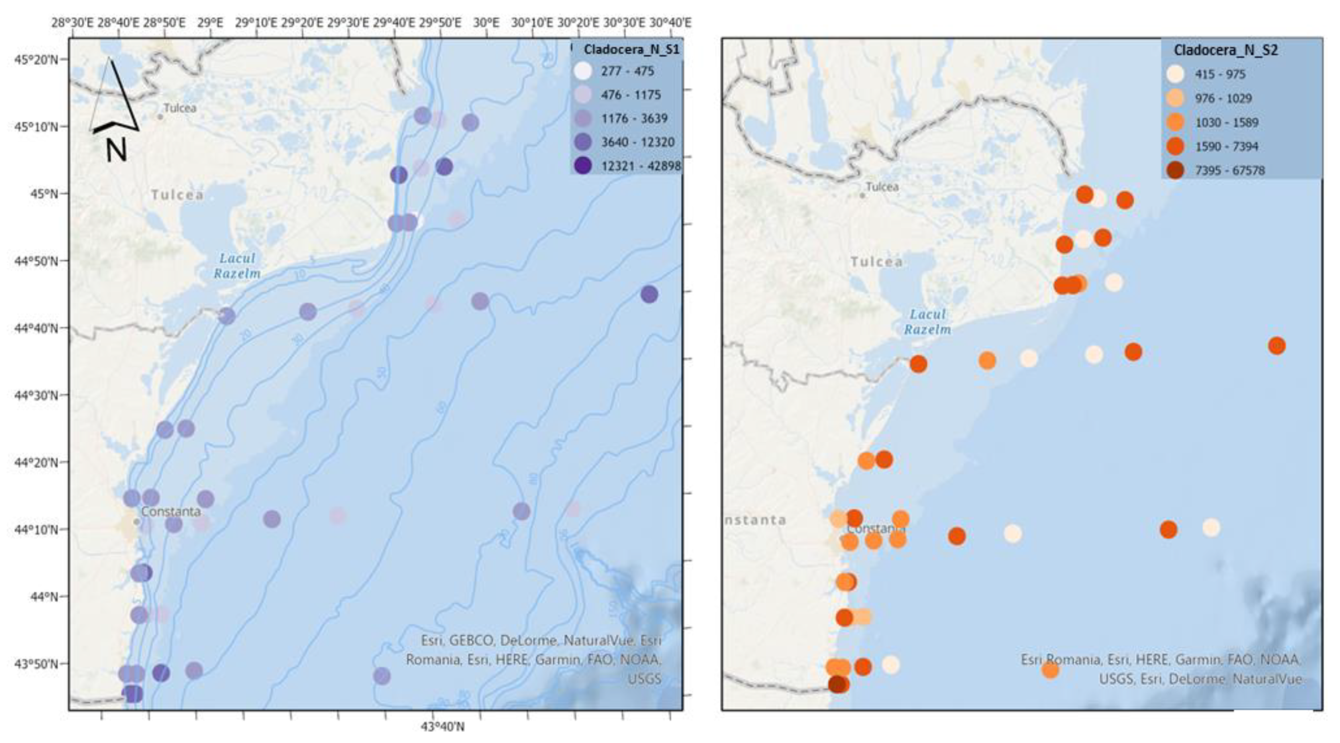
22]. In both scenarios, cladocerans reach high densities, indicating, in certain areas, a sustainable trophic base for higher trophic levels adapted to predicted temperature and salinity conditions (
Figure 10).
Meroplankton can represent a substantial part of the zooplankton community, with its contributions to total density being greater in estuarine areas [
23]. The main characteristic of shallow areas is the abundance of meroplankton organisms, which can produce real explosions in the water mass, constituting the dominant elements in the zooplankton composition [
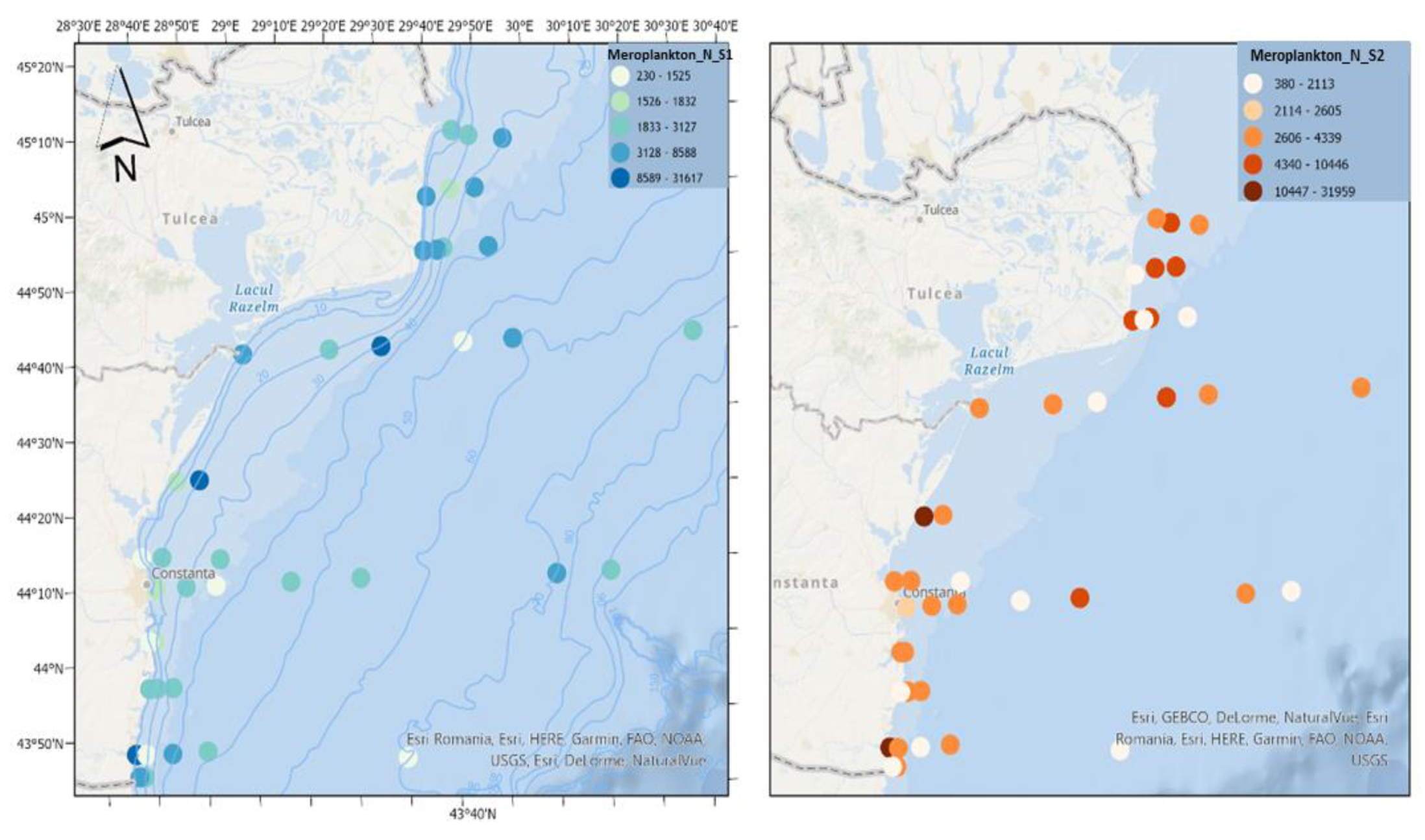
24]. In the two scenarios, the meroplanktonic component reaches similar density values (
Figure 11). It can compete for resources with holoplanktonic species and serves as a food source for planktonic predators [
25]. On the other hand, climate change can affect the reproduction and recruitment of benthic invertebrates, affecting the abundance of meroplankton [
26].
The category “Other groups” consists of the appendicular
Oikopleura dioica, the chaetognath
Parasagitta setosa and the mysid
Mesopodopsis slabberi, the latter being much less represented and with a low frequency of occurrence. Being important as food for fish larvae, appendicularians bridge the gap between small primary producers and higher trophic consumers [
27].
Parasagitta setosa can exert high predation pressure on copepods and thus compete with the food available for the larval stages of fish [
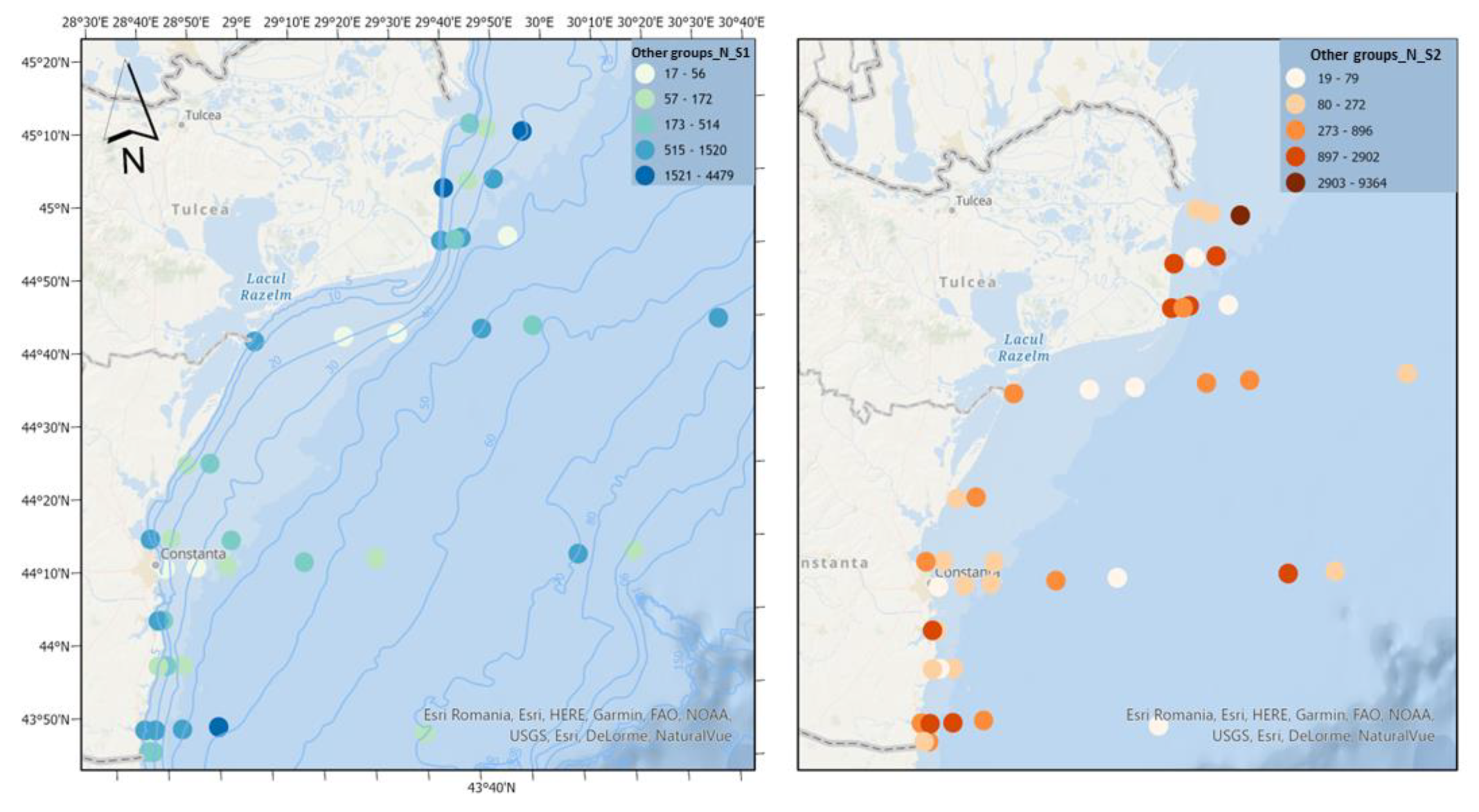
28]. Scenario 2 experiences a significant increase in the density of the "Other groups" category, in contrast to scenario 1, which shows minimal growth (
Figure 12). This difference is primarily driven by the overall phytoplankton density.
4. Discussion
Zooplankton is crucial for moulding planktonic ecosystems, controlling phytoplankton growth, and transferring energy from lower-trophic animals to higher ones [
29]. The local community structure is shaped by local environmental parameters, such as water temperature, pH, salinity, trophic state, or combinations of these factors (i.e., the species-sorting hypothesis) [
30]. Furthermore, zooplankton is significantly influenced by nutrients in the environment [
31,
32], having an indirect impact on zooplankton by having a top-down effect on phytoplankton [
33].
The assessment of physico-chemical parameters is required to analyse the water quality and energy succession of an aquatic environment. The physico-chemical parameters of an aquatic ecosystem affect phytoplankton and zooplankton diversity and abundance [
34]. A significant issue for the aquatic food web is eutrophication which is caused by high phosphate and nitrate concentrations. Algal blooms prevent phytoplankton and other organisms from getting enough oxygen, which can lead to an organism's demise, leading to a decline in biodiversity and water body toxicity [
35].
Fuzzy-Logic Cognitive Mapping (FCM) was developed as early as 1986 as a way to structure expert knowledge using a systems programming approach that is "fuzzy", thought to be similar to how the human mind makes decisions. Because of their flexibility, FCMs were created to examine perceptions of an environmental problem or to model a complex system where uncertainty is high and there is little empirical data available.
The model created by us within the project has 89 components and 203 linear connections (positive or negative) between them, connections that human thinking cannot make simultaneously to allow a clear analysis of the evolution of the pelagic component of the marine ecosystem
, the concentrations of silicates and nitrates affecting the densities of meroplankton and copepods. Copepods are usually known as ammonium-excreting microorganisms, hence positive associations between copepods and nitrite (NO
2) and nitrate (NO
3) have also been documented [
36,
37].
A comprehensive approach to improving water quality must take into account the macroenvironmental elements influencing it as well as the participation of many stakeholders in water management decisions [
38,
39,
40,
41,
42,
43,
44].
The results obtained with the help of FCM are further the basis of the system knowledge and the generation of hypotheses for the predictions in different scenarios developed by us based on the specialized literature.
In the next stage, based on the collected data and supervised machine learning (ML) algorithms from ArcGIS, we obtained the models and proliferation scenarios of phytoplankton and zooplankton, indicators of eutrophication in the waters of the Romanian Black Sea coast. Zooplankton demonstrates a wide range of ecological strategies, dominance patterns, and effects on ecosystems in marine habitats. It is difficult and still early to adequately express this variation in conceptual and mathematical frameworks [
16].
The advantage of ML over traditional statistical techniques, especially in earth sciences and ecology, is the ability to model numerous variables, which may be non-linear, with complex interactions between them and sometimes with missing values [
45,
46].
Several comparative studies have already shown that ML techniques can outperform traditional statistical approaches in a wide variety of problems in earth sciences and ecology. However, this requires a careful analysis which is why we chose to create the semi-quantitative model based on FCM in the preliminary stage [
46].
In both scenarios developed using ML, high densities of
N. scintillans were observed. This dinoflagellate produces impacts on the ecosystem in coastal areas around the world [
47], generally in the spring and summer seasons when it registers high abundances, establishing the blooming phenomenon of the species [
48]. The blooms generated by
N. scintillans are closely related to food availability, especially to the presence of diatoms, which it consumes, controlling the dynamics of this phytoplankton group [
37]. The phenomenon causes mortalities among fish, many of which are of economic importance, as well as marine invertebrates due to the accumulation of high levels of ammonia in the water [
49].
N. scintillans plays an important role in marine food chains [
48], feeding on a wide variety of organisms such as phytoplankton (mainly diatoms), eggs, larvae and faecal pellets of crustaceans, as well as with other mesozooplanktonic organisms [
50]. High densities of this dinoflagellate can limit local population growth of copepods, not only when they compete for food, but also because they feed on their eggs and nauplii [
51].
The run scenarios for copepods showed an increase in abundance, which can generate a positive impact on the environment, especially for pelagic fish. There is evidence that recruitment is highly dependent on copepod production [
52], high prey availability encourages recruitment and early survival by maximising food intake and growth throughout the larval stage of life in the plankton [
53]. These findings offer information regarding the presence of plankton prey, which can lead to a more efficient management decision regarding fisheries. Although it is not conclusive to conclude that zooplankton biomass is the only factor affecting fish recruitment, high prey abundance available at the time of fish spawning will promote recruitment [
17]. Still, there remains a possibility that the increase in temperature could lead to a reduction in copepod species diversity and a shift toward smaller-sized copepod communities [
54]. Additionally, another potential risk associated with copepods, the predominant zooplankton in oceans, involves their influence on seawater through the introduction of distinct polar lipids known as copepodamides. These lipids can stimulate toxin production and bioluminescence in harmful dinoflagellates [
55].
Meroplankton recorded similar abundance values in both scenarios. The ecological significance of planktonic larvae is two-fold: they are a dispersal stage for benthic organisms [
56], determining the potential of benthic species to colonise adjacent habitats, but they can also constitute a major portion of zooplankton [
57], potentially competing for resources with holoplanktonic species, and serving as food source for planktonic predators [
25,
28]. Larval movement is a crucial biophysical mechanism in benthic ecosystems that, in advection-dominated environments, can result in a spatial decoupling between local community production and settlement [
59].
“Other groups” category does not know a very large development from a quantitative point of view, in contrast to scenario 2 where a much greater increase in density is noted. Species belonging to this group act as a crucial link in the food chain between pico- and nanophytoplankton and larger zooplankton like fish larvae [
60], copepods, ctenophores [
61], jellyfish [
62].
P. setosa grows and matures at high copepod density and greater temperature, indicating that temperature and food are the main factors influencing
P. setosa growth in the Black Sea [
63] as observed in scenario 2.
Jellyfish and ctenophores, acting as predators of young fish and zooplankton, indicate ecosystem health decline or human-induced stress from overfishing and the reduction of zooplankton predators when they form blooms. This scenario might lead to an excessive presence of gelatinous zooplankton, causing a considerable adverse impact on fish recruitment [
17]. The appearance of gelatinous zooplankton indirectly affects the ecosystem by boosting phytoplankton and detritus levels, consequently reducing water quality, triggering hypoxia, and causing harm to fish and other wildlife [
64].
The nutritional quality of phytoplankton significantly influences the entire food web, especially through its relationship with zooplankton. Therefore, to ensure efficient stock management and optimize fishing resources, it's crucial to consistently assess the trophic interactions among phytoplankton, zooplankton, and fish within fishery management practices [
65]. Diminished future phytoplankton biomass will favor the development of gelatinous food webs. Hence, employing the trait-based modelling framework showcased here becomes a potent method for uncovering fresh perspectives on the impact of climate change on zooplankton and their crucial role in global marine ecosystems, effectively linking planktonic organisms with fish populations [
66].
Elevated organic matter levels could potentially initiate alterations in the nitrogen-to-phosphorus ratio, significantly affecting the growth and diversity of phytoplankton and various marine algae. These imbalances might lead to shorter trophic food webs, reduced predator numbers, and potential decreases in biodiversity [
67].
Author Contributions
Conceptualization, L.L. and E.B.; methodology, L.L. and E.B.; software, L.L.; validation, L.L. and E.B.; formal analysis, L.L. and E.B.; investigation, L.L. and E.B.; resources, L.L., L.B., E.P., F.T., O.V., E.B.; data curation, L.L., L.B., E.P., F.T., O.V., E.B.; writing—original draft preparation, L.L. and E.B.; writing—review and editing, L.L., L.B., E.P., F.T., O.V., E.B; visualization, L.L., L.B., E.P., F.T., O.V., E.B.; supervision, L.L. and E.B; project administration, L.L. and E.B; funding acquisition, E.B. All authors have read and agreed to the published version of the manuscript.
Figure 1.
Map of the study area. The square shows the location of the sampling sites on the Romanian coastline (A) and the position in the Black Sea region (B).
Figure 1.
Map of the study area. The square shows the location of the sampling sites on the Romanian coastline (A) and the position in the Black Sea region (B).
Figure 2.
Annual variation of temperature, salinity and nutrients - Romanian Black Sea coast, 2008-2018, warm season.
Figure 2.
Annual variation of temperature, salinity and nutrients - Romanian Black Sea coast, 2008-2018, warm season.
Figure 3.
Phytoplankton composition from the Romanian Black Sea coast, 2008-2018, warm season.
Figure 3.
Phytoplankton composition from the Romanian Black Sea coast, 2008-2018, warm season.
Figure 4.
Zooplankton composition from the Romanian Black Sea coast, 2008-2018, warm season.
Figure 4.
Zooplankton composition from the Romanian Black Sea coast, 2008-2018, warm season.
Figure 5.
Distribution of Noctiluca scintillans from the Romanian Black Sea coast, 2008-2018, warm season.
Figure 5.
Distribution of Noctiluca scintillans from the Romanian Black Sea coast, 2008-2018, warm season.
Figure 6.
Fuzzy Cognitive Map (FCM) – the result of applying statistically significant correlations between abiotic factors (blue), phytoplankton species (grey) and zooplankton groups (magenta) and N. scintillans (orange) – warm season, 2008-2018.
Figure 6.
Fuzzy Cognitive Map (FCM) – the result of applying statistically significant correlations between abiotic factors (blue), phytoplankton species (grey) and zooplankton groups (magenta) and N. scintillans (orange) – warm season, 2008-2018.
Figure 7.
The importance of explanatory variables from the models made by Machine Learning - Forest-based Classification and Regression algorithm for the ecosystem of the Romanian Black Sea coast, 2008-2018, warm season.
Figure 7.
The importance of explanatory variables from the models made by Machine Learning - Forest-based Classification and Regression algorithm for the ecosystem of the Romanian Black Sea coast, 2008-2018, warm season.
Figure 8.
Density of N. scintillans in scenario 1 (BAU) (left) and 2 (RCP2.6) (right) – ML prediction for warm season (2042).
Figure 8.
Density of N. scintillans in scenario 1 (BAU) (left) and 2 (RCP2.6) (right) – ML prediction for warm season (2042).
Figure 9.
Density of Copepoda in scenario 1 (BAU) (left) and 2 (RCP2.6) (right) – ML prediction for warm season (2042).
Figure 9.
Density of Copepoda in scenario 1 (BAU) (left) and 2 (RCP2.6) (right) – ML prediction for warm season (2042).
Figure 10.
Density of Cladocera in scenario 1 (BAU) (left) and 2 (RCP2.6) (right) – ML prediction for warm season (2042).
Figure 10.
Density of Cladocera in scenario 1 (BAU) (left) and 2 (RCP2.6) (right) – ML prediction for warm season (2042).
Figure 11.
Density of meroplankton in scenario 1 (BAU) (left) and 2 (RCP2.6) (right) – ML prediction for warm season (2042).
Figure 11.
Density of meroplankton in scenario 1 (BAU) (left) and 2 (RCP2.6) (right) – ML prediction for warm season (2042).
Figure 12.
Density of other groups in scenario 1 (BAU) (left) and 2 (RCP2.6) (right) – ML prediction for warm season (2042).
Figure 12.
Density of other groups in scenario 1 (BAU) (left) and 2 (RCP2.6) (right) – ML prediction for warm season (2042).
Table 1.
Performance of models and importance of explanatory variables – 2008-2018, warm season.
Table 1.
Performance of models and importance of explanatory variables – 2008-2018, warm season.
| |
Model |
R2 (validation) |
T$@$(oC) |
S$@$(‰) |
PO4$@$(µM) |
DIN$@$(µM) |
Total FPK density$@$(cel/L) |
| 1 |
Normal - Total phytoplankton density (cells/L) |
0.17 |
26 |
45 |
17 |
12 |
- |
| 2 |
Normal –Noctiluca scintillans density (ind/m3) |
0.66 |
14 |
27 |
37 |
21 |
2 |
| 3 |
Normal – Copepoda density (ind/m3) |
0.56 |
29 |
20 |
25 |
24 |
2 |
| 4 |
Normal – Meroplankton density (ind/m3) |
0.55 |
28 |
31 |
24 |
15 |
2 |
| 5 |
Normal – Cladocera density (ind/m3) |
0.71 |
28 |
18 |
24 |
25 |
5 |
| 6 |
Normal – Other groups zooplankton density (ind/m3) |
0.67 |
26 |
22 |
17 |
23 |
12 |
| 7 |
Blooms - Total phytoplankton density (cells/L) |
0.91 |
20 |
20 |
37 |
23 |
- |
| |
Blooms – Noctiluca scintillans density (ind/m3) |
0.95 |
27 |
13 |
42 |
12 |
6 |
| 9 |
Blooms –Copepoda density (ind/m3) |
0.80 |
36 |
13 |
22 |
10 |
20 |
| 10 |
Blooms –Meroplankton density (ind/m3) |
0.87 |
24 |
18 |
22 |
18 |
18 |
| 11 |
Blooms – Cladocera density (ind/m3) |
0.99 |
22 |
9 |
25 |
18 |
27 |
| 12 |
Blooms – Other groups zooplankton density (ind/m3) |
0.98 |
30 |
8 |
16 |
19 |
27 |
