1. Introduction
The cement industry is one of the most energy-intensive industrial sectors today [
1]. In addition, the increase in industrial cement production creates the need to reduce energy and polluting components. The optimization of the cement production process, whether it concerns the ratio of materials in the mill [
2,
3,
4,
5,
6,
7,
8,
9,
10,
11,
12,
13,
14] or the fineness of cement [
15,
16,
17] or the improvement of the occurrence of failures [
18,
19,
20] or the reduction of the environmental footprint [
3,
21] or the optimization of the kiln’s lubrication [
22] or the reduction of the energy consumed [
21,
23,
24,
25,
26,
27] is based on two main approaches: Optimization through mathematical models where the operations in the cement plant are expressed through linear or non-linear relationships[
2,
8,
9,
11,
12,
17,
18,
19,
21,
26,
27,
28] and optimization through improvement of the system architecture and control process [
3,
4,
5,
6,
7,
10,
13,
14,
15,
16,
18,
20,
23,
24,
25,
26]. Due to the complexity of the production process in cement production and the different parameters that need to be taken into account (temperature, exhaust gas, material quality, etc.), the optimization of the overall cement production is necessary to satisfy as many conditions as possible. Two important steps in the cement production process are the grinding of the material in the mill and the processing of the material in the kiln.
The mill’s optimal operation is challenging due to its mechanism complexity, the constant slurry composition changes, and raw material grinding. In addition, the problems caused by overloading or underloading of the mill cause damage to the equipment which increases over time depending on the mill operator and the strength of the materials [
2]. The mill operator is therefore an important factor in the optimum operation of the mill in terms of energy consumption and cement quality as well as the useful life of the equipment. The non-linear relationships will be expressed by machine learning models with optimized parameters. However, this is not sufficient as optimized operation of the cement plant is not guaranteed. For this reason, it is important to introduce the machine learning models into an optimization function to derive a final optimized operation.
In this work, the system operator determines the objective function to be optimized rather than having a predetermined form. To be more precise, the operator establishes whether a parameter is to be within predetermined bounds or converge to a desired value. It is also defined whether the optimization will be maximized or minimized. The data are extracted from a Mongo database that contains information about the Greek cement factory’s kiln or mill. The objective is to predict seven (7) non-manipulated variables for the mill and three (3) non-manipulated variables for the kiln. The manipulated variables are those that the user can determine, whereas the non-manipulated variables are those that are calculated using linear or non-linear relationships between the manipulated variables. Since there are fifty-four (54) features for the mill and twenty (20) features for the kiln, two feature selection algorithms named Recursive Feature Elimination with Cross-Validation (RFECV) and Sequential Feature Selector (SFS) are used to select the most suitable features for training the machine learning models. More specifically, the best features are the common features selected by these two algorithms. Machine learning models are used to compute the non-manipulated variables because it is well known that the relationships between parameters in a complex process are almost unlikely to be linear. The optimal model is selected from among the regressors KNN, Linear, LGBM, XGBoost, GBR, CatBoost, Random Forest, and TTR based on the target variable’s case.
Before training the models and selecting the best of them, the user has the right to intervene and define the optimal parameters of the model. Then the user switches to the next interface and specifies the bounds or the target value together with the monotonicity. This study adds to a dynamic optimization system in an actual Greek cement factory where the operator or the system defines the active Artificial Intelligence (AI) models and the expert determines the objective function. Essentially, the current method utilizes mathematical models to combine equipment optimization through mathematics and user participation to create a hybrid model. The machine operator’s experience should be combined with the AI model training and the optimization process. The expert concerns the data distribution and then utilizes the data clustering method. The clusters of data are divided based on the concept drift of the data. The occurrence of concept drift means that certain points of data signal a new distribution of data or a new behavior of data. In the next step, the Intelligent Decision Making System (IDMS) interacts with the expert user. The user establishes the bounds of the not-manipulated parameters both for the kiln and the mill. The recommendations of the method are shown on the dashboard, where the user can determine whether they are appropriate values. Furthermore, the user possesses the ability to specify the parameters of the active prediction AI model. After training, the system can, nevertheless, choose the active AI model based on the NRMSE metric. Last but not least, the form of the objective function is defined by the user. In general, human-system interaction is the foundation of the entire system.
2. Related Work
More than half a century has passed since the first attempts to automate the process of cement production towards automating the cement production process through the interconnection of the various parts of the factory with computer systems [
29]. Many works have dealt with the optimal management of industrial units and cement plants. By exploiting exhaust gases [
30] and utilizing high temperatures in the rotary kiln shell [
31], thermal energy loss and the release of polluting gases are reduced. Nitrogen oxides in the kiln also contribute to the worsening of the environmental impact of cement industries [
32,
33]. The optimization of water, heat, and electricity was addressed in [
34] and the optimization of nitrogen dioxide in [
35] as well as in work [
36]. The temperature of the lime kiln was investigated in [
37]. However, individual parameter optimization does not create an overall reliable solution that optimizes the cement plant as a whole system. In work [
21], several objective functions were created to reduce energy consumption, gas emission intensity, and economic cost. In the same work, nonlinear or linear relationships between parameters are not considered, thus machine learning models could play this role. In work [
38] the combination of AI and optimization methods is used to determine the optimal composition of the mix concerning the cement mortar materials. The study [
39] considers the slurry’s optimal composition and the properties relevant to cement production. In the work [
40], AI and optimization models are used to find the optimal point for environmental, economic, and engineering objectives in silica concrete production. The proportion of materials in concrete also occupied the work [
41]. Machine learning models are created using nine (9) parameters. These models, in combination with heuristics, establish a system of proposals regarding the "recipe" of the concrete. The work [
42] used machine learning models and an optimization algorithm to determine the content of free calcium oxide in cement clinker. In [
43] a method for the management of big data coming from the installations of a cement plant is proposed. The analysis of the data and their presentation is carried out using an Enterprise resource planning (ERP) system. However, neither innovative optimization models nor AI models are involved in the process. The same idea is also the basis of the work [
44], where more emphasis is placed on optimizing the presentation of the results in the UI (User Interface) than on the data processing method. In this case, simple statistical methods are used. The work [
45] proposes a method to optimize cost, energy, and material supply using PLC-based controllers. However, neither machine learning models nor an advanced mathematical optimization model are used.
The architecture and design of the mill and separator are altered to create an Advanced Process Control (APC) system in work [
46], which uses a costly method to improve the mill feed and cement fineness without allowing the user to provide feedback on the quality of the results in the control panel. In the current study, the user defines the optimization process via the dynamic dashboard. In [
47] the problem in the optimal management of information systems in the cement industry is identified in terms of the system’s acquisition cost, usability, quick response time, and KPIs management. The work [
48] aims to optimize the kiln and the quality of the clinker extracted from the kiln. Although AI models are being used and considerable data points are being taken into account, advanced optimization methods are not being employed and the models are retrained with data of varying distributions. In the current study these issues are solved. This work is an extension of the study [
49], where now the objective function is dynamic, the parameters of the objective function have been enriched in both the mill and the kiln and the method has been integrated into a cement production process control system. Last but not least, in the current study the user can determine the retraining of the models through the control table if he/she observes from the visualization of the data distribution based on the clustering method that there is a concept drift in the data. In our case, we have a small improvement in the performance of the algorithms after changing the data understanding in energy consumption.
3. Materials and Methods
3.1. System Overview
In general, the developed system is based on the production needs of the cement industry of Thessaloniki and aims to provide manufacturing industries with an autonomous, cognitive, intelligent and reliable framework. Based on embedded mechanisms of collective cognitive thinking, the goal is to efficiently use and reuse raw resources and energy. Furthermore, the system aims to monitor, control, and optimize the production process performance while minimizing human intervention.
The system is a digital technology unit which utilizes an Industrial Internet-of-Things (IoT) subsystem to collect real-time data from sensors during the production process. The system also employs algorithmic Artificial Intelligence and decision-making tools to analyze the collected data, all to optimize the production process through predictive analysis. The industery facilities which will interact with the system are demonstrated in
Figure 1.
3.2. System Architecture
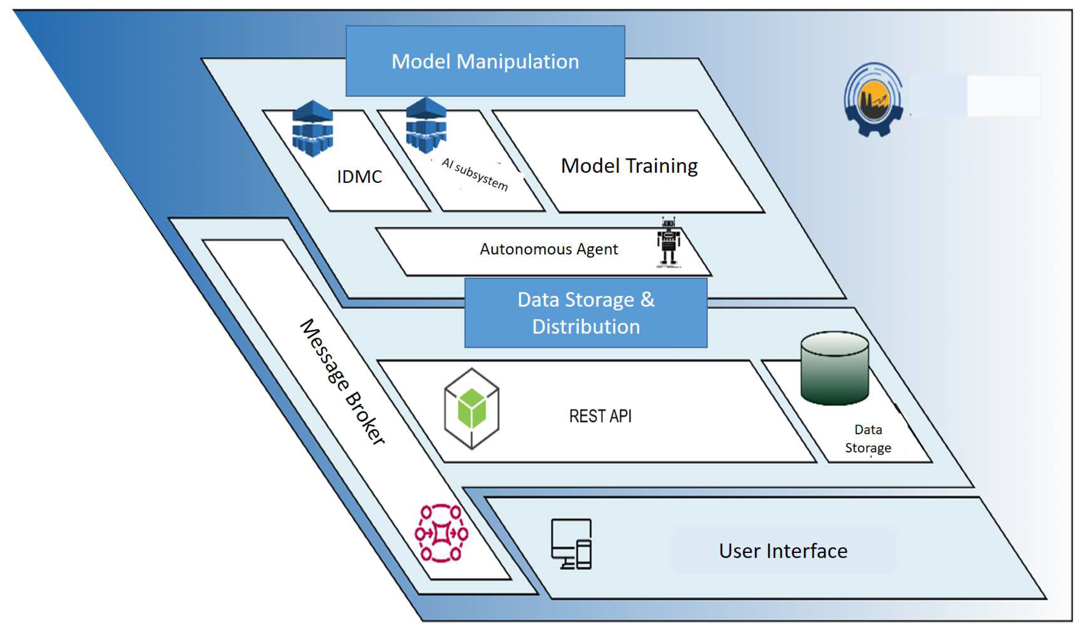
The main responsibility of the physical layer - factory is to send sensory data to the system to optimize production. The exchange of this data is achieved by using MQTT (Message Queuing Telemetry Transport) protocol requests which are received by the message broker. The message broker has direct communication with all the algorithmic tools/services in the system and thus forwards the data received to them.
The REST API (RESTful Application Programming Interface) is the intermediary for any action to store or retrieve data from the database. This is how the algorithmic tools communicate: i) With the message broker for data requiring real-time exchange and ii) with the REST API to retrieve and/or store data in the database. The services of the system include the IDMS and AI Subsystem tools which exchange data between them through the message broker. These services utilize predictive models which are trained and acting during production. The message with the predictive data is also traced by the API which will store the data in the database for future use. The autonomous agent tool is either a real user or an intelligent system. After getting the evaluation of the acting AI model (training parameters, performance metrics, historical data, historical predictions), the agent decides if the retraining routine should be called so the re-training parameters are entered into it.
3.3. System Sub-modules
The sub-modules developed for the system, consist of tools and technologies that are necessary for its operation. Using Docker allows the creation of images for each of these subunits and ensures that they work uniformly in every environment. The system sub-modules are listed below:
3.3.1. The Mongo Database
The Mongo Database server sub-module is the one that hosts the database that is utilized by the system to store the data necessary for its operation. The Mongo database image includes the Mongo server and all the necessary dependencies for its operation. The Dockerfile for the database defines the sequence of actions to be performed to install and configure the Mongo database server inside the Docker container.
3.3.2. User Interface (UI)
The graphical interface is one of the most important tools of the system, as it enables the user to manipulate the system functions. It is hosted by the Web Server, which includes all the necessary dependencies for executing the interface code and communicating it with the various sub-modules of the system. The Interface, which is configured for the respective sub-module, is a central platform for collaboration between the different sub-modules of the system. It offers a set of methods and functions, allowing the other sub-modules of the system to exploit its methods for training, prediction, optimization, and decision-making in an automated and coordinated manner. Finally, the interface aims to ensure maximum flexibility and efficiency of the process by ensuring that the methods are extensively used by the other sub-modules of the system.
3.3.3. Mosquitto MQTT Broker
The Message broker sub-module is responsible for the real-time communication between the different sub-modules of the system. It includes all the necessary dependencies required for its operation and the security of the communication. Cedalo’s Mosquitto Management Center is a modern graphical environment that enables organized control and management of customers connected to an IoT architecture through the Mosquitto message broker, provided by Eclipse. It offers several features aimed at improving the process of managing and monitoring the information generated by customers. Some of these features include real-time data visualization, organizing customers into hierarchical groups, the ability to perform searches based on various criteria, and extracting data for further processing. Finally, Cedalo’s Mosquito Management Center offers easy configuration of security levels, allowing the definition of access rights for customers. The image for the message broker includes the Mosquitto message broker, an MQTT protocol server, and all the necessary dependencies for its operation. The Dockerfile for Mosquitto defines the commands to install and configure it.
3.3.4. Mosquitto Management Center
The image of the Management Center includes its implementation and all the necessary dependencies for its operation. The Dockerfile defines the commands to be executed to install and start the Management Center application. The system’s services are divided into two main elements as follows.
3.3.5. AI subsystem
The AI subsystem is responsible for applying the models generated by the retraining algorithm as well as generating predictions and making decisions. The AI subsystem combines the historical data with the recently collected data to provide real-time predictions of the values of the variables in the IDMS.
3.3.6. Intelligent Decision Making System (IDMS)
The IDMS utilizes the methods provided by the AI subsystem and promotes the optimal values to the other sub-modules of the system. The DE optimization method is used to compensate the system for the optimized values of the manipulated variables as derived from the combination of the optimization method of the AI methods and the feature selection methods.
3.3.7. Receiving Real-Time Data
The implementation of real-time communication between the system and the physical layer is based on cloud tools and services. Azure Databricks and Azure Data Lake are two critical tools for managing and processing large volumes of data. Data Lake is designed for data storage, supporting the ability to store data in various formats. Data are stored in the parquet format. This format is efficient in storing column-oriented data and provides high performance in reading and processing data. Azure Databricks is a powerful data processing and analysis tool. By leveraging Databricks, an algorithm for reading and sending data was developed using the Python programming language. In
Figure 3 the Databricks interface is shown. The data are sent via HTTP request to the system’s server. The server receives the data from Databricks and verifies whether the received values exist or not. The new values received are stored in the system’s beta database while those that exist are ignored. In this way, data loss is minimized and duplicate values are avoided, to achieve smooth and seamless real-time communication.
3.4. Data Description
3.4.1. Cement Mill
The data used were from a period of almost three (3) years. Specifically, it consisted of the months of 11/2020-12/2022 and 06-07/2023. The data prepossessing involves the elimination of the data points where there is no mill operation. In the same context, the data relating to the first twenty minutes (20 minutes) after starting the mill operation were also discarded due to the instability of production in these intervals. The manipulated variables are the following: The mill feed, the grinding pressure, the separator speed, the water flow, the mill inlet pressure, the mill outlet pressure, and the mill inlet temperature. The prediction models are connected with the mill energy consumption, the mill differential pressure, the separator energy consumption, the mill exit temperature, the environmental dust, and the mill vibrations as well as the cement finesses indices (Blaine and Residue).
3.4.2. Cement Kiln
The data used was throughout approximately six (6) months. Specifically, they relate to the period 01/12/2022 - 12/06/2023. The first step in the data pre-processing process involved cutting out the intervals of kiln inactivity. Kiln operation was defined as those intervals during which the kiln feed rate exceeds 135 t/h. The manipulated variables are the Total feed, the Preheater and the Solid Fuel Feed. The kiln prediction models are associated with models the calculated nitrogen oxides, the kiln amps, and the preheater carbon dioxide.
3.5. Feature Selection Methods
For feature selection, we applied an automated selection procedure in which we combined two well-known methods: RFECV and SFS. This combined approach allowed us to identify a set of features that are highly relevant to the predicted variable. The subset resulting from the combination of the RFECV and SFS results is then introduced as input for training the prediction models.
3.5.1. Recursive Feature Elimination with Cross-Validation (RFECV)
The features are initially given weights according to an estimator such as the coefficients of a model. In the RFE method, features are eliminated iteratively by considering smaller sets of features in each iteration. The importance of each feature depends on some metric such as the pseudo-efficiency [
50]. The least significant features are excluded from the selected features. The process is terminated when the desired features reach the desired number. The RFECV method additionally uses the stratified validation method in the selection of mapping features [
51].
3.5.2. Sequential Feature Selector (SFS)
This method is based on the greedy approach where at each step a feature is added or removed based on the overlap method [
52]. However, it only considers the independent variables in the training process and not the dependent variable to be predicted [
53].
3.6. Artificial Intelligence Methods
3.6.1. Multi-layer Perceptron Regressor (MLP)
By calculating the partial loss derivatives at each MLP Regressor training cycle, the parameters are updated. In the loss function, the model parameters are reshaped using a regularization term to avoid overfitting [
54]. For the MLP model, the best value for the hyperparameter hidden layer sizes was chosen among (1,), (2,), (5,), (1,1), (2,2) and (5,5), where the number of hidden layers and the number of neurons in each is determined. Also, tanh was set as the activation function, blogs as the optimization method (solver), 108 as the maximum number of iterations, and the regularization parameter
was set equal to 0, as these options seemed to give generally better results than the default values of these hyperparameters, based on preliminary experiments.
3.6.2. Gradient Boosting Regressor (GB)
By creating a progressively additive model through an estimator, it is possible to optimize random differentiable loss functions. The negative slope of any given loss function is mapped to a regression tree [
55]. For the GBR model the best value for the max depth hyperparameter was chosen between the values 5, 10, and 15, for the number of estimators hyperparameter among the values 50, and 100, while for the min_samples_split hyperparameter, the value 8 was set instead of the default, which is 2, as it seemed to give better results based on preliminary experiments.
3.6.3. Light Gradient Boosting Regressor (LGBM)
LightGBM is a type of GB Regressor where discrete buckets sort continuous values based on histogram algorithms. Thus it speeds up the training process while being a computer memory-friendly process [
56]. For the LGBM model, the best value for the max depth hyperparameter was chosen among the values 5, 10, and 15, and for the number of leaves hyperparameter among the values 8, 10, and 12.
3.6.4. Extreme Gradient Boosting Regressor (XGBoost)
The XG Boost algorithm is a variant of the GB algorithm and is based on trees to create regression models using gradient boosting. The advantages of the XG Boost algorithm are summarized in the intelligent splitting of trees into short leaf nodes, and randomization [
57].
3.6.5. Random Forest Regressor
A large number of decision trees create a meta-evaluator random forest. Each of the decision trees is mapped to different subsets of the dataset. The average error improves the predictive accuracy while controlling for overfitting. The size of each subset of the sample is expressed by the hyperparameter max, otherwise, each tree is generated from the entire dataset [
58]. For the Random Forest Regressor model, the best value for the hyperparameter number of estimators was chosen among the values 10, 15, 20, 25, 50, and 100, and for the hyperparameter max depth among the values 1, 2, 5, and 10.
3.6.6. k-nearest neighbors (KNN) Regressor
In this method, uniform weights are used. That is, in each local neighborhood of a point the distribution of candidate solutions is uniform. Depending on the case, weights are given to nearby points or distant points [
59]. For the KNN the best value for the hyperparameter number of neighbors was chosen among the values 5, 10, 50, 100, and 200, and for the hyperparameter leaf size among the values 20, 30, 50, and the hyperparameter weights between the values uniform and distance.
3.6.7. Linear Regressor
In linear regression analysis, there is the dependent variable to be predicted and the independent variable that is known. The model is essentially a linear correlation between the dependent and independent variable or independent variables [
60].
3.6.8. Cat Boost Regressor
Combining decision trees with the greedy approach and gradient boosting theory to combine several weak models at each step of the algorithm is the main idea behind the CatBoost method. Each new tree improves its performance by learning from the errors of previous trees until the intercept of the performance metric is not reduced [
61].
3.6.9. Transformed Target Regressor (TTR)
Used for non-linear transformations of the dependent variable. Either a transformer such as the Quantile Transformer or its inverse is used [
62]. For the CatBoost model and the TTR model, their hyperparameters were set equal to their default values.
3.7. Clustering Data Method
3.7.1. k-means
The k-means algorithm is an unsupervised machine learning algorithm which clusters data points that have some similarity. The number of clusters is predefined and the method sets the center of each cluster (centroid). This value is representative of each cluster [
63]. Depending on the distance of each point to the centroids, the algorithm assigns it to the least distant cluster.
3.8. Normalised Root Mean Squared Error (NRMSE)
The NRMSE is a variant of the RMSE. The RMSE is calculated according to Equation (
1). The smaller the RMSE, the closer the predictions are to the actual prices.
where
is the actual value of variable and
its predicted value. The
n reflects the number of observations. The values that have a different measurement from the active forecasts cannot be compared and therefore the construction of a metric that can be applied to all variables is necessary [
64]. This metric is the NRMSE, which weights the mean squared error in terms of mean, standard deviation, difference between maximum and minimum, or interquartile range. When the NRMSE is equal to 0 it means that the predictions coincide with the actual values [
65]. In the current study, the mean square error is normalized with respect to the standard deviation. The normalized form of the mean squared error is mainly useful in large statistical samples and in cases of heterogeneous outcome variables. The NRMSE is calculated according to Equation (
2). The
is the standard deviation of variable’s distribution.
3.9. Objective Function
The objective function is also the KPI of the application. Essentially the degree of optimization of the cement production process is user-oriented. The user dynamically determines the form of the key performance indicator which is equal to the objective function as Equation (
3).
where
is the weight the user assigns to the variable when it is selected the variable to be within constraints. The
and the
is equal to either the value 0 or 1 depending on whether the upper and lower ends of the constraints are selected respectively. The
and
are both Boolean variables which are equal to
False until the active value of the variable is either less than the minimum threshold (
minimum) or greater than the maximum threshold (
maximum). These thresholds are set by the user.
is a binary variable where it is equal to -1 if the user chooses to maximize the current variable and 1 if the user chooses to maximize the current variable since DE minimizes the objective function.
equals the weight the user gives to the monotony of the corresponding term in the objective function.
is the weight given if we choose the variable to have values close to a target value. In case we choose a target value, both the choice of bounds and monotony are disabled.
expresses the target value,
expresses the actual value of the variable at the current step in the optimization process,
expresses the standard deviation and finally
expresses the mean value of the variable from the data.
where
Wn that equals a power of 10 if the user chooses to set it within a predefined range or equals 0 if the user does not choose this variable. Also, the upper and lower edge of the variable’s bounds is specified by the user. The
is a variable where it is equal to the negative sign in maximization and equal to the positive sign in minimization. The value of the weight in this case exponentially amplifies the existing weight. This case is expressed by the first term of equation
3 and it is activated if the Boolean variable is true. The monotony is not needed, in the case where the user selects to minimize the distance of the variable from a target value. The weight of each variable is determined by the user again.
If the selected variable
belongs to manipulated variables, it receives the current value within the predefined bounds (
), and if the variable is non-manipulated then the value of the variable depends on the linear or non-linear relationships between the selected variables. These variables were determined by the feature selection algorithms while the dependent value is estimated by the active machine learning models (
) as it is represented in Equation (
4).
3.10. Differential Evolution (DE)
The DE is a metaheuristic of continuous iterations until the candidate solution is judged to be the best. The initial assumptions about the problem are few or none and the space of candidate solutions is very large. In general, DE is considered a stable and reliable optimization algorithm. The origination of the method is in work [
66]. The studies [
67,
68,
69,
70] prove that the DE is the most stable and reliable optimization algorithm. The DE method belongs to the stochastic evolutionary methods, chooses the best among numerous candidate solutions, and has only three (3) parameters. The existence of a few parameters is one of its main advantages. The main disadvantage of the method is that the selection of the best parameter values is a hard task. Finding the optimal values of the control parameters can be time-consuming and difficult, especially for difficult problems. For these reasons, researchers study and develop new advanced DE variants that exhibit adaptive or self-adaptive control parameters. The control parameters are adjusted based on the feedback received during the search process [
71]. In our case, the bound intervals of the manipulated variables are the minimum and maximum values from the data. We set the maximum number of iterations to three hundred (300) which is quite a high number, while the population size of candidate solutions is equal to five (5). The number of iterations is high since the problem is likely to be multidimensional and the value of iterations depends on the ability of the algorithm to find candidate solutions [
72]. The optimization method is represented in the Equation (
5).
where
Ne is the number of parameters,
x = { , ..., } is the vector containing the candidate solution areas
of all elements and
is the value of element i. In addition,
is the behavioral constraint, of K variables. At each step, the algorithm generates a new candidate solution by combining the existing solutions of the previous step. The candidate solutions give the objective function the best value, which is either the highest or lowest according to monotony, at each step. The procedure is iterative until the satisfaction of a predefined criterion [
72].
4. Results
4.1. Data Clustering
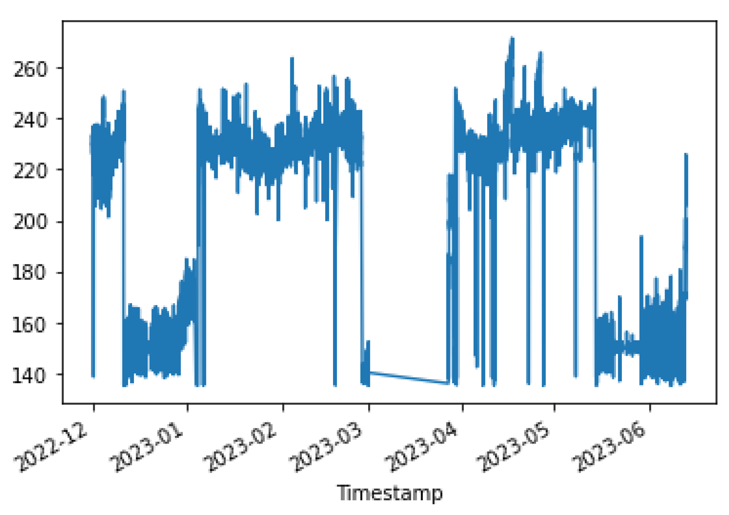
The data in the kiln feed exhibits two distinct distributions over time. As can be observed from
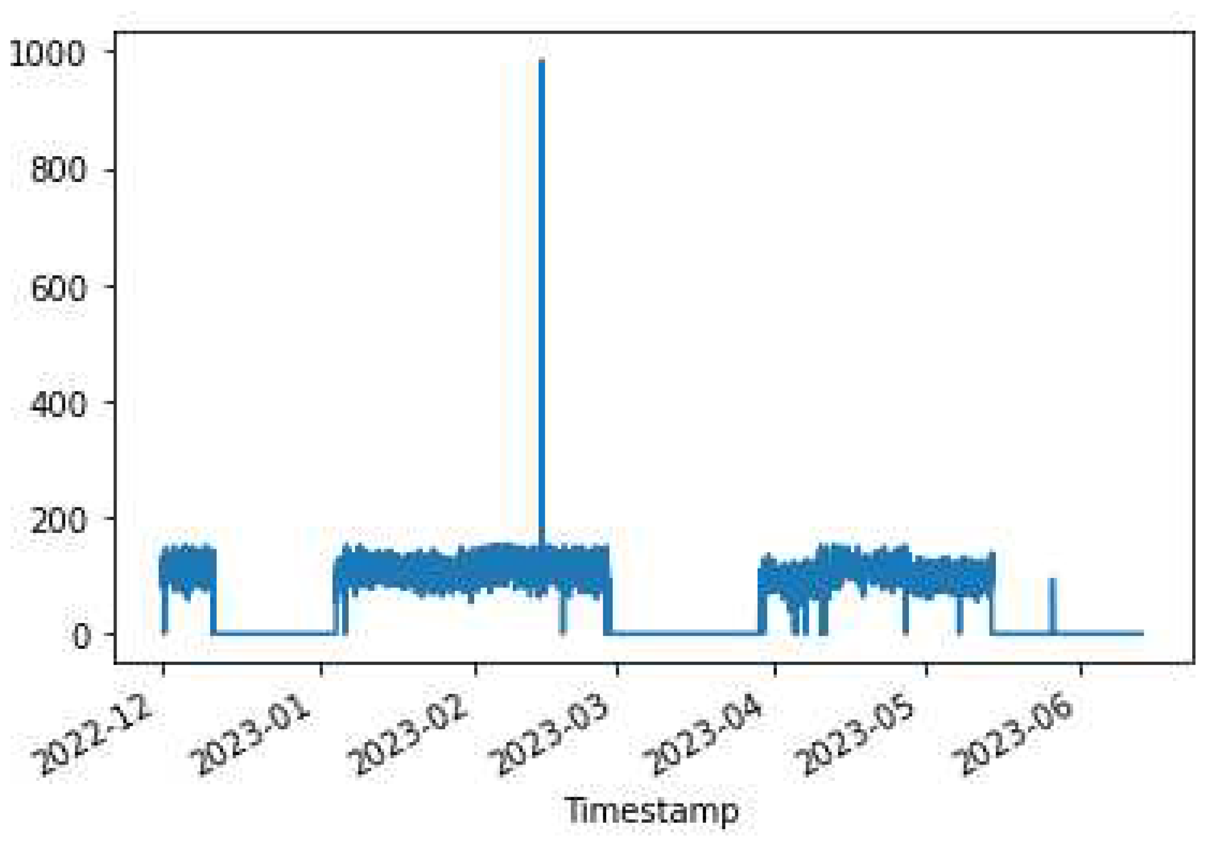
Figure 4, the first distribution describes the feed between 140 and 160 tons, while the other describes the feed between 220-240 tons. The Kiln ambers distribution is drawn in
Figure 5. Kiln ambers are almost zero (0) during the lowest kiln feed period, which is observed to indicate that the kiln is not operational. The model which will be created will predict the non-operational periods even when the kiln loading exceeds 135 t/h.
4.2. AI subsystem Results
Feature selection methods RFECV and SFS seek the features of the data which create the best-performing model. The intersection of the results of the two methods, i.e., the common features, are those with which the machine learning models were trained. These characteristics are represented in
Table 1 for the mill and in
Table 2 for the kiln.
During the training of machine learning models, the one which performs best is always selected. This is not an easy process, as the performance of the models often depends on the hyperparameters of the algorithms and their numerous combinations. Therefore, it is necessary to find a way to tune the hyperparameters to the set of hyperparameters of the best-performing model [
73]. The Python library scikit-learn with the GridSearchCV method provides a hyperparameter tuning tool in an automatic and fast way [
74].
Table 3 and
Table 4 represent the results obtained in each step for the cement mill and kiln respectively. After training the AI regression models the represented results show the best-performing model for each variable as well as its test NRMSE and its optimal parameters.
The results in
Table 5 and in
Table 6 are derived after applying the feature selection methods combined with the clustering method for the cement mill and kiln respectively. Indeed, the clustering method achieves the segregation of data into operational periods. The NRMSE of the models is examined in the case where there are two behaviors in the data. The total NRMSE is obtained by summing the squared errors of all classes in a single square root in the numerator, which is equal to the deviations between the actual value and forecast, and the denominator, which is equal to deviations between the actual value and the mean value.
Observing
Table 4 and
Table 6, the results imply that in the kiln although there are two different behaviors in the kiln feed and in the kiln amps the model retraining brings no improvement in NRMSE and all cases marginally worsens it. For the case of the mill (
Table 3 and
Table 5), the results in some variables are improved and more specifically for the non-manipulated variables Mill Differential Pressure, Environmental Dust Blaine, and Residue however the improvements of RNMSE are again marginal.
4.3. Cement Mill Optimization Results
4.3.1. Experimental Set Up
To ensure that the optimized results apply to the cement plant, it will be set the bounds for the non-manipulated variables as to differ by ten (10) percent from the value of the non-manipulated variable in the last data point. The timestamp of the last data point is 7/16/2023 5:00:00 PM. The Mill Feed value at the last data point is equal to 104.2245, so the constraint is the interval between 93.79 and 114.64. The weight assigned is equal to 1 and is the smallest as the mill feed should not significantly affect the other optimization parameters. In this point, the current study differs from the previous one ([
49]) where the mill feed was the most important variable. On the other hand, the current study is similar to the previous approach [
49] as target values were set for Blaine and Residue, namely 4900 for the former and 2.3 for the latter. The weight given to these parameters is equal to 10.
The Mill Differential Pressure, the Environmental Dust, and the Mill Exit temperature are parameters added to this work. More specifically the last value for mill differential pressure is equal to 21.67 and the optimal value will be found within the interval [19.503, 23.837]. The weight to be given is equal to and it is desirable to be maximized. For the environmental dust, the last point value is 6.14, so the optimal solution is between 5.53 and 6.76. One main goal is the improvement of the environmental footprint, so the environmental dust should be minimized. The weight given is equal to 100. The mill exit temperature should be maximized to save energy. The last data point value was equal to 91.87 and the optimum value will be in the range [82.68,101.06]. The weight assigned to the variable is equal to .
The power consumption of the mill and separator and the vibrations of the mill are the most important variables in the optimization process. For this reason, they are given weights of , and respectively. The last point value for mill power consumption in Kilowatt (KW) was 2079.82, for separator power consumption in KW was 94.421, and for mill vibration was 1.102364 mm/s. The intervals within which the optimization intervals will be found are [1871.84, 2287.81], [84.97, 103.86], and [0.99, 1.21] respectively.
4.3.2. Setting parameters from the UI
Figure 6 demonstrates the user’s initial selection in the Control Panel. The optimization will apply to either the mill or the kiln. Of course, the user has the right to undo his selection and return to this step.
Figure 7 represents the user’s ability to specify the parameters which will be included in the objective function. If the user does not select any parameter, then the weight to be given to it is set equal to zero (0). The user has the right to select the constraints of the variable together with its monotony or a target value for this variable. In the case where the constraints are chosen, he/she may not choose a target value and vice versa. Furthermore, if the target variable is selected, the user cannot specify the monotony.
Finally, the user selects the parameters of the DE optimization method as it is represented in
Figure 8. These parameters are important in the efficiency of the method. More specifically, the population size determines the initial population while the number of iterations is the upper limit of steps of the algorithm.
4.3.3. Cement Mill Results
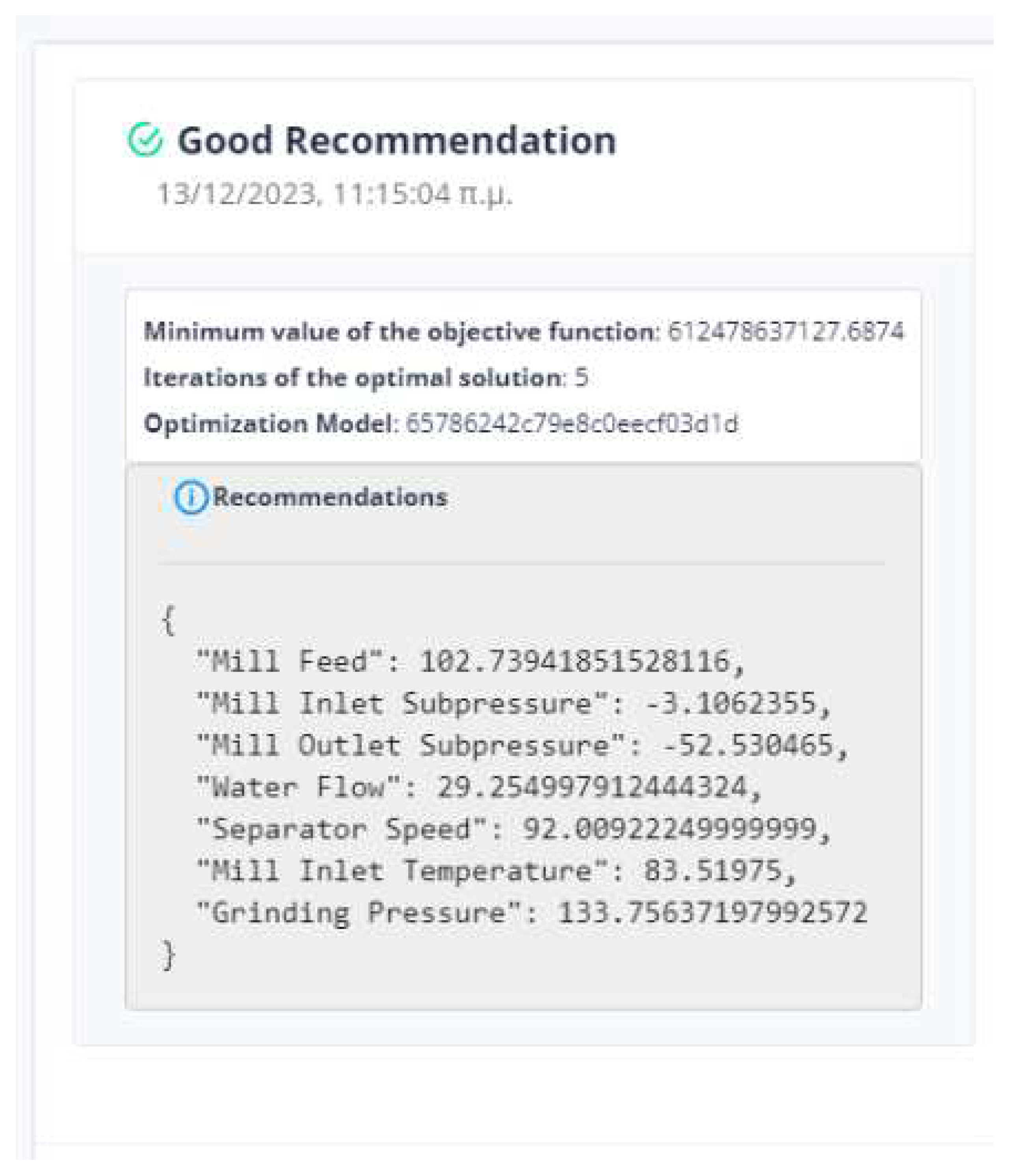
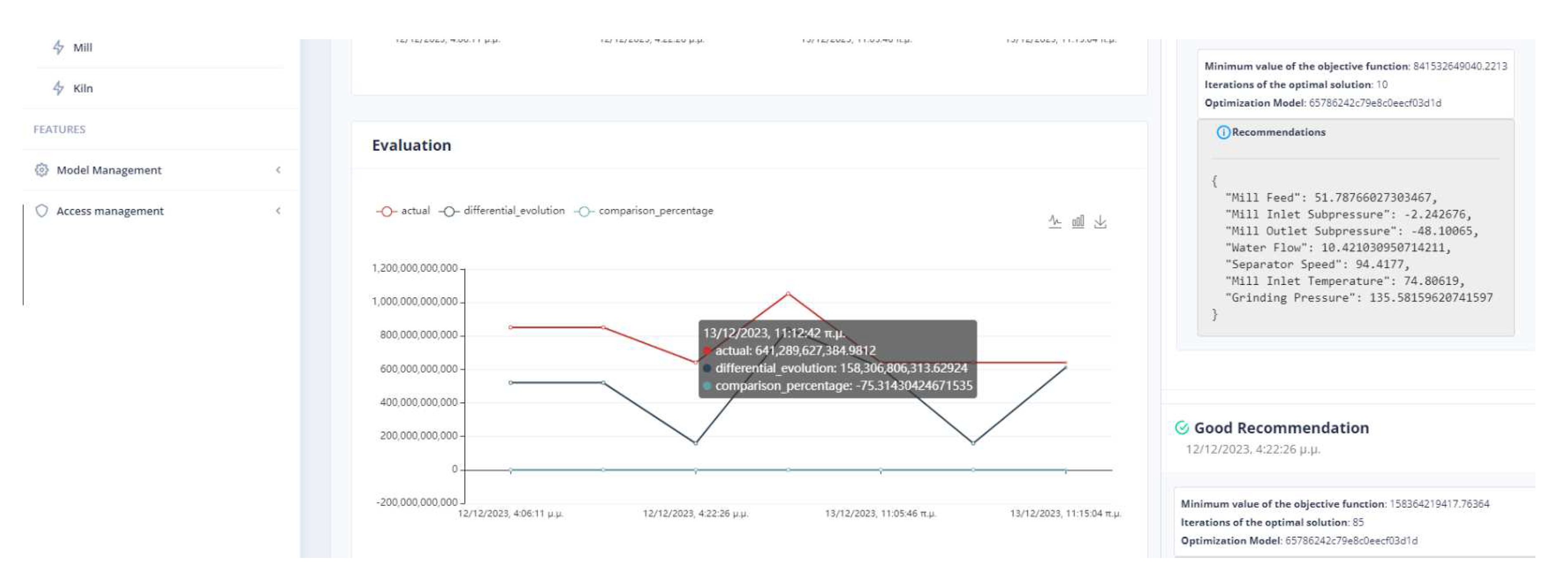
The evaluation of the optimization is carried out by comparing two variables. The first quantity is the value of the objective function as obtained by applying the DE method and the second is the calculation of the objective function by giving the values of the parameters equal to the values at the last data point. If the DE achieves a lower value compared to the last data point then we have an acceptable recommendation of optimal operation as in
Figure 9.
Six (6) trials of the DE function were conducted at different times. In all cases, the value of the function from DE is less than the value of the function from the active data point. The actual result of the optimization is the percentage change in the active value of the function relative to the value from DE. In our example, the value of the objective function improves the process by about 75%. as it is drawn in
Figure 10.
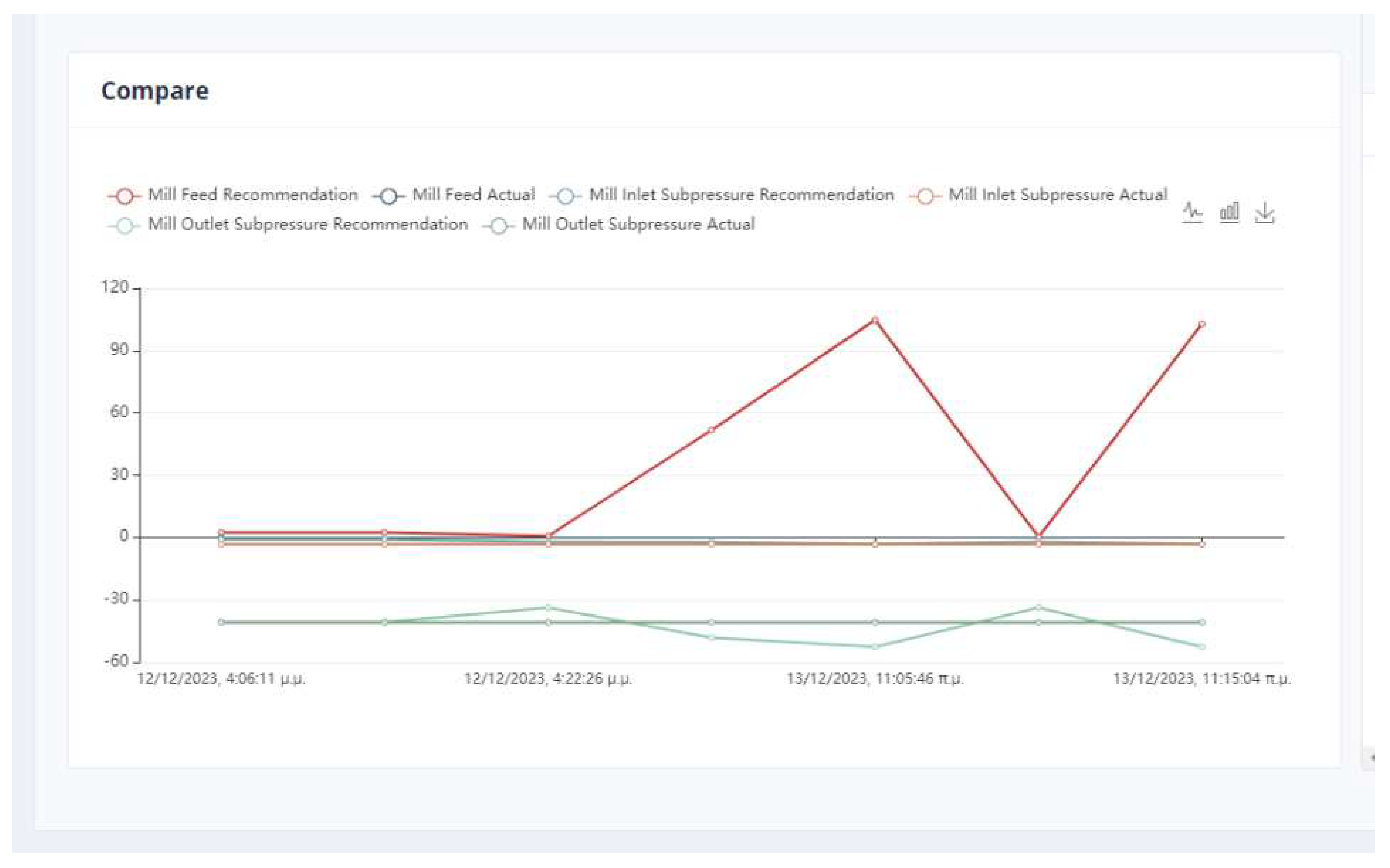
An important issue in the optimization process is the proximity of the proposed values to the effective values so that the system can transition to them without crashing. In
Figure 11 it can be seen that the feed of the mill is far from the recommended value. Although in the rest of the cases, the mill will operate without any problems, the possible sudden changes are an issue that must be taken care of by the user.
The effectiveness of the method was assessed with non-manipulated variables using inference from the best-performing machine learning models. The models’ predicted values, when the proposed values from the IDMS are used as input, fall within the acceptable limits established in the DE, as indicated in
Table 7.
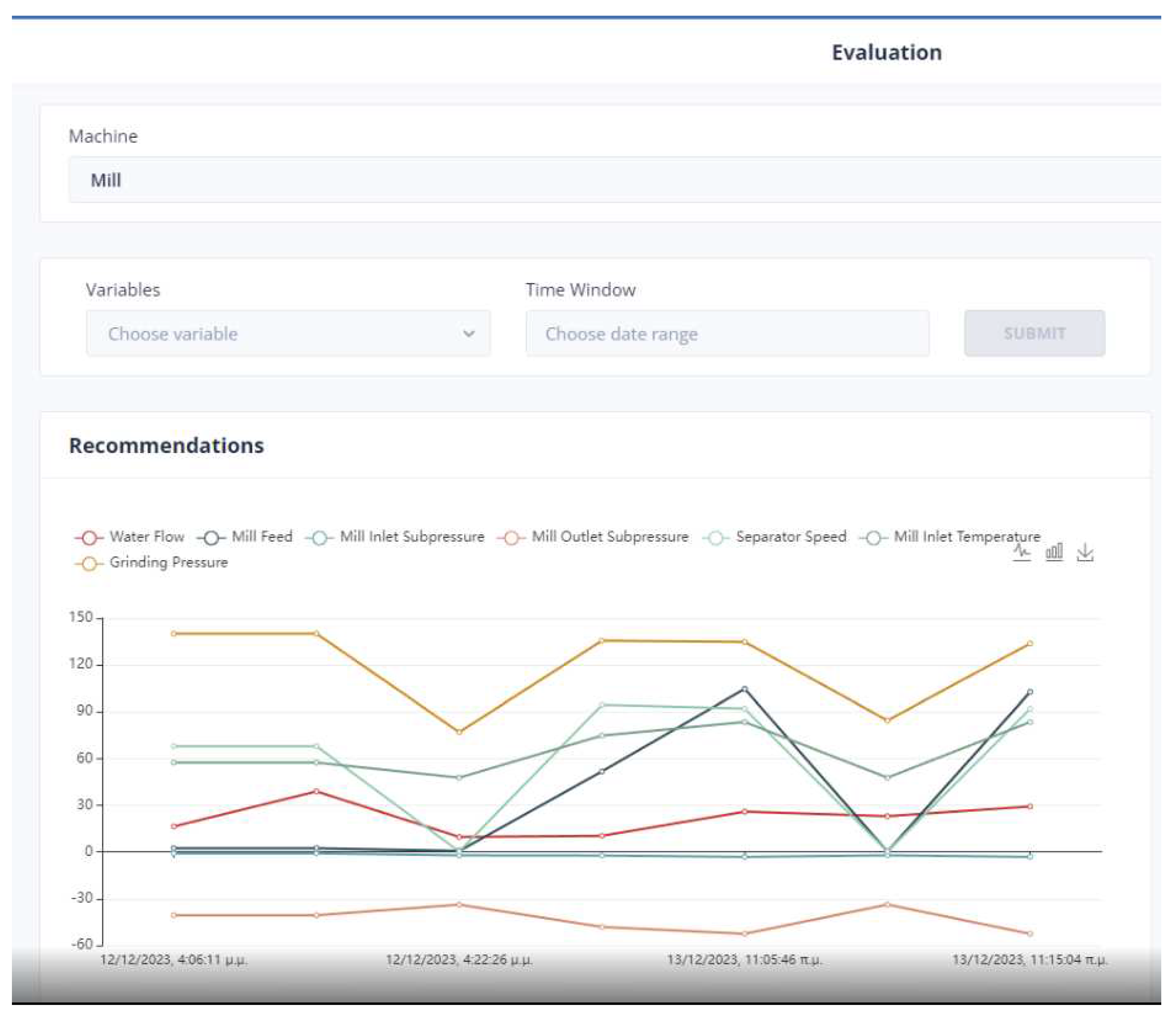
The system can retain past recommendations and demonstrate them to the user as in
Figure 12. In this way, it is possible to judge indirectly whether the behavior of the system has changed. In addition, the user can determine the time range of the data which will be utilized during the process.
4.4. Cement Kiln Optimization Results
4.4.1. Experimental Set Up
The kiln is optimized based on both three manipulated variables and three non-manipulated variables predicted by the models. The objective function considers the two types of variables along with their respective weights. Any fluctuation in the variables that are part of the objective function will be 30% close to its last data value. Specifically, the maximum and minimum values will be 30% greater and less than the last data value respectively.
The total feed is given a weight equal to 10 and must be within the limits of the interval [174.285, 323.673]. It is also the only variable that is maximized. The variable PreheaterO2 shall be within the interval [0.606, 1.126]. It is minimized and gets a weight of 10. Finally, the Solid fuel variable is restricted to the interval [3.963, 7.359], has a weight equal to 10, and is minimized.
The Calculated Nox variable is minimized and given a weight of 1000. It falls within the range of 0.0002278 and 0.000423. Kiln Amps, on the other hand, is also minimized and weights 10000. It is constrained to be in the range of 92.205 and 171.238. Lastly, Preheater CO is minimized with a weight of 1000. It is within the range of 0.0255 and 0.04748. These variables are not manipulated and are bounded within their respective ranges.
4.4.2. Setting parameters from the UI
In the kiln, the operator makes the corresponding settings to the dashboard in the mill shown in
Figure 6,
Figure 7 and
Figure 8.
4.4.3. Cement Kiln Results
The system’s recommendations to the user are recorded in the dashboard as shown in the
Figure 13. The application user can refer to earlier system recommendations where another objective function was probably involved in the optimization.
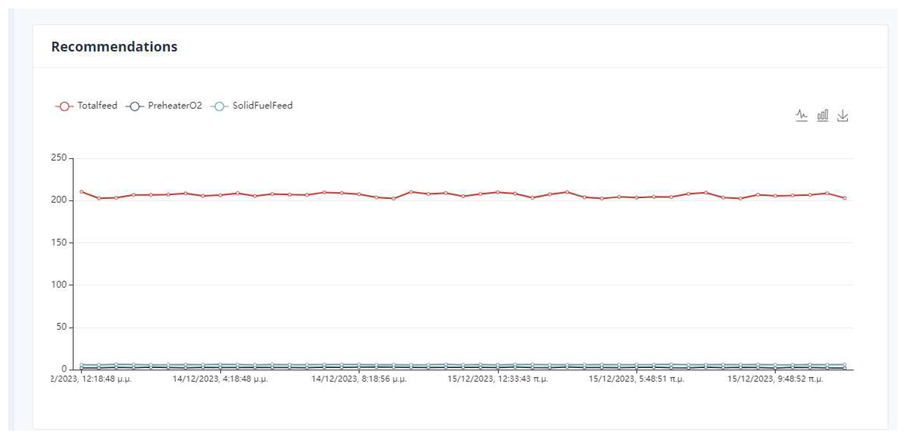
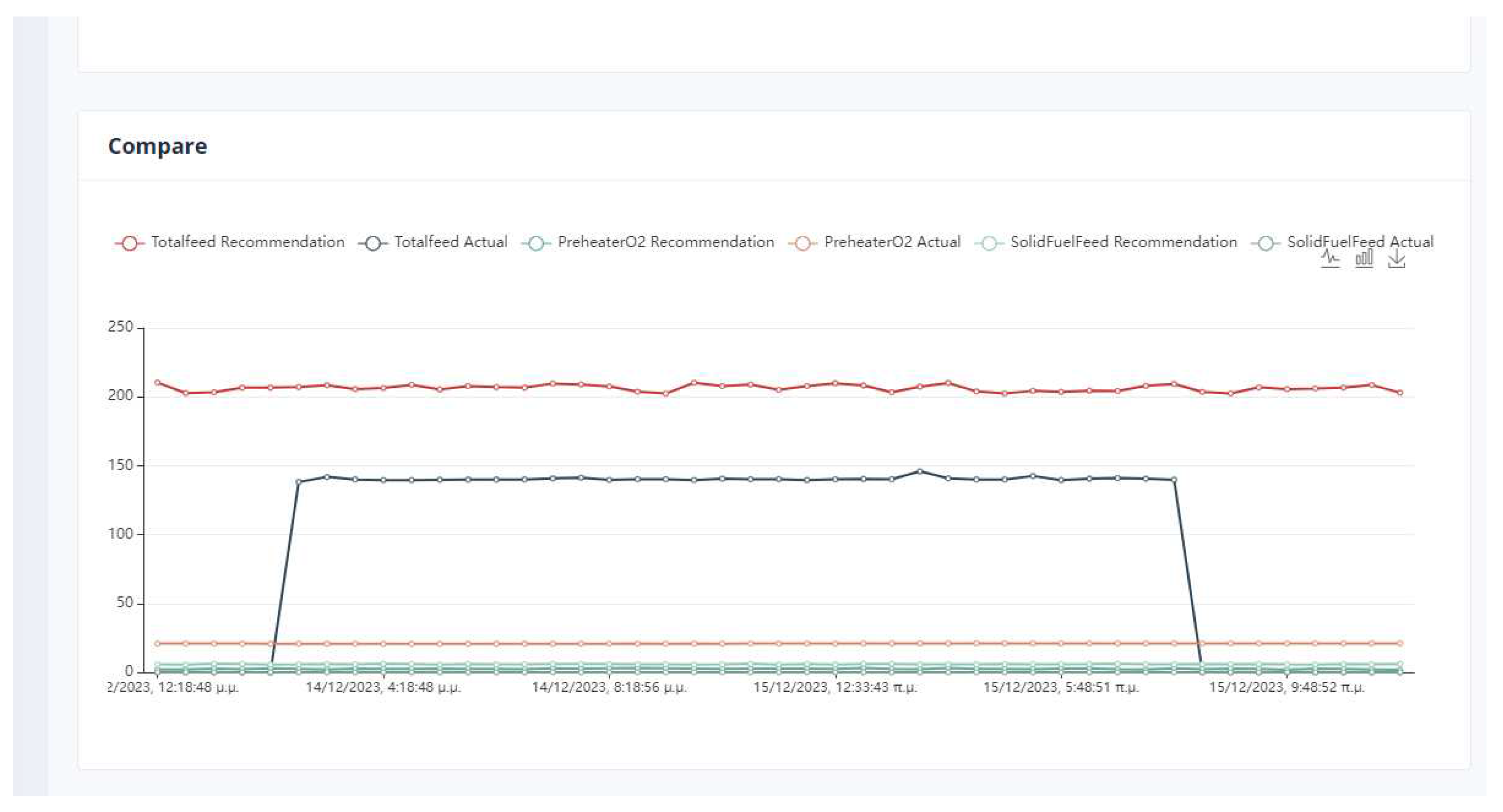
Observing
Figure 14, it can be concluded that the recommendations optimize the system. For example, the total feed is increased relative to the current value. The user has to decide if it is feasible to switch to this production point. The same is observed for the PreheaterO2 variable where the active value is higher than the recommended value.
5. Discussion
The cement industry is presently one of the most energy-intensive sectors. In addition, cement is an important material in the construction sector. It is essential to combine with the maintenance of the quality of cement expressed by Blaine and residue, the reduction of energy consumption, and the devaluation of the environmental footprint of the plants. The cement production has many parameters which are either calculated by deterministic functions or measured by special sensors. Also, during production, there are either manipulated variables which can be defined by the cement plant user, non-manipulated variables, or uncontrolled variables. The non-manipulated variables play an important role in the optimization of the production and the uncontrollable variables are getting values within a predefined range. The non-manipulated variables of either the mill or the kiln depend linearly or non-linearly on both the manipulated variables and the uncontrollable variables. The relationships between these parameters are difficult to determine, so feature selection methods are used to find the most relevant parameters. Machine learning models are then trained to incorporate the correlation between each dependent variable and independent variables.
The current study concerns a cement industry in Greece that has several plants. Each cement plant has different stresses and the maintenance works of each machine change the data distribution of each parameter. For the above reasons, it is imperative to retrain the AI models if the production conditions change. However, many times the data distribution changes as the production conditions are dynamic e.g., there are parameters such as internal or external temperature. In this work, the expert is concerned with the data distribution and if a sharp concept shift is observed, the data is clustered into groups and retrained. The overall NRMSE resulting from all clusters is the final measure. With the data provided by the factory, no improvement in the results of the cement mill models was observed. In addition, no improvement was observed in any of the predicted variables of the kiln. The optimization of the production parameters in the cement mill and the cement kiln was derived from a dynamic objective function in which the expert operator can assign monotony or value-weighting to each manipulated or non-manipulated variable. According to the use cases that came from the operators of the cement plant, the objective function is improved compared with the value that gets the objective function if the values of the variables came from the last database entry.
An important limitation of the work is the lack of historical data that could further improve the results. In a future extension of the work, more and more advanced clustering methods should be applied. In addition, more pre-processing may be needed on the data. Last but not least, another limitation is the fact that many times the current mill or kiln operation values cannot be switched abruptly to the proposed values derived from the IDMS. This point should also be taken into account in future extensions of the work. At this stage, the specific issue must be taken care of by the user of the system.
Authors should discuss the results and how they can be interpreted from the perspective of previous studies and of the working hypotheses. The findings and their implications should be discussed in the broadest context possible. Future research directions may also be highlighted.
6. Conclusions
In this work, the optimization method applied in a cement plant in Greece was combined with feature selection algorithms, AI methods, and behavioral data separation. In addition, a major innovation was the definition of the objective function by the user where each selection from the control matrix created an additional term in a linear form function. The non-linear relationships of the functions were expressed by the AI models.
The constraints of the non-manipulated variables were specified to be 10% to 30% close to the active variable. The final results depicted in the dashboard showed that the value of the objective function decreases with the application of DE concerning the active value of the objective function from the last data point in both the mill and the kiln of the cement plant .
7. Patents
This section is not mandatory, but may be added if there are patents resulting from the work reported in this manuscript.
Author Contributions
Conceptualization, O.M. and N.K.; methodology, N. K., M.Sk., O.M., M.L., I.P., C.K. P.G. and N.K.; software, M.Sk., C.K., D.Tzi., M.O., M.L., and N.T; validation, M.Sk., C.K., D.Tzi., M.O., M.L., N,T., P.G., and N.K.; formal analysis, M.Sk., N.K.; investigation, M.Sk., O.M., A.T., I.P., N.K., C.K.; resources, O.M., A.T., D.I., D.Tzo. and M.St.; data curation, N.T., M.O., D.Tzi., M.Sk., N.K.; writing—original draft preparation, M.Sk; writing—review and editing, M.Sk., O.M., D.I., N.K..; visualization, M.O., D.Tzi.; supervision, N.K., D.I., D.Tzo. and M.St.; project administration, O.M., A.T., D.I., D.Tzo. and M.St.; funding acquisition, D.I., D.Tzo. All authors have read and agreed to the published version of the manuscript.
Acknowledgments
This work is partially supported by the SIROKO project co-financed by the European Regional Development Fund of the European Union and Greek national funds through the Operational Program Competitiveness, Entrepreneurship and Innovation, under the call RESEARCH – CREATE – INNOVATE (project code: T2EDK-04748).
Conflicts of Interest
The authors declare no conflict of interest.
Abbreviations
The following abbreviations are used in this manuscript:
| APC |
Advanced Process Control |
| AI |
Artificial Intelligence |
| DE |
Differential evolution |
| ERP |
Enterprise resource planning |
| GB |
Gradient Boosting Regressor |
| IDMs |
Intelligent Decision Making System |
| IoT |
Internet-of-Things |
| KNN |
k-nearest neighbors |
| KPIs |
key performance indicators |
| KW |
Kilowatt |
| LGBM |
Light Gradient Boosting Regressor |
| MDPI |
Multidisciplinary Digital Publishing Institute |
| MLP |
Multi-layer Perceptron Regressor |
| MQTT |
Message Queuing Telemetry Transport |
| NRMSE |
Normalised Root Mean Squared Error |
| PLC |
Programmable Logic Controller |
| REST API |
RESTful Application Programming Interface |
| RFECV |
Recursive Feature Elimination with Cross-Validation |
| SFS |
Sequential Forward Selection |
| TTR |
Transformed Target Regressor |
| UI |
User Interface |
| XGBoost |
Extreme Gradient Boosting Regressor |
References
- Zhang, W. , Maleki A., Khajeh M.G., Zhang Y., Mortazavi S. M., Vasel-Be-Hagh A. A novel framework for integrated energy optimization of a cement plant: An industrial case study. Sustainable Energy Technologies and Assessments 2019, 35, 245–256. [Google Scholar] [CrossRef]
- Tang, J. , Qiao J., Liu Z., Zhou X., Yu G., Zhao J. Mechanism characteristic analysis and soft measuring method review for ball mill load based on mechanical vibration and acoustic signals in the grinding process. Minerals Engineering 2018, 128, 294–311. [Google Scholar] [CrossRef]
- Campos, H.F. , Klein N. S., Marques F.J., Bianchini M. Low-cement high-strength concrete with partial replacement of Portland cement with stone powder and silica fume designed by particle packing optimization Journal of Cleaner Production 2020, 261, 121228. [Google Scholar] [CrossRef]
- Alsobaai A., M. Effect of Feed Amount and Composition on Blaine and Residue in Cement Mill.
- Altun, O. Simulation aided flow sheet optimization of a cement grinding circuit by considering the quality measurements. Powder technology 2016, 96, 1242–1251. [Google Scholar] [CrossRef]
- Schnatz, R. Optimization of continuous ball mills used for finish-grinding of cement by varying the L/D ratio, ball charge filling ratio, ball size and residence time. International journal of mineral processing 2004, 74, S55–S63. [Google Scholar] [CrossRef]
- Čáchová, M. , Kot’átková J. , Koňáková D., Vejmelková E., Bartoňková E., Černỳ R. Properties of Lime-cement Plasters with the Addition of a Pozzolana Procedia Engineering 2016, 151, 127–132. [Google Scholar] [CrossRef]
- Anwar, S. , Afrizalmi L. L. Optimization of Production Planning Using Goal Programming Method (A Case Study in a Cement Industry) Int. J. Appl. Math. Electron. Comput 2015, 3, 90–95. [Google Scholar]
- Altun, O. , Benzer H. Selection and mathematical modelling of high efficiency air classifiers Powder technology 2014, 264, 1–8. [Google Scholar] [CrossRef]
- Genç, Ö. Optimization of a fully air-swept dry grinding cement raw meal ball mill closed circuit capacity with the aid of simulation. Minerals Engineering 2015, 74, 41–50. [Google Scholar] [CrossRef]
- Ichalal, D. Marx B., Maquin D., Ragot J. Observer design for state and clinker hardness estimation in cement mill. In IFAC Workshop on Automation in Mining, Mineral and Metal Industries, MMM 2012; Publishing House: CDROM, 2012. [Google Scholar]
- Wang, X.-Y. Analysis of hydration and strength optimization of cement-fly ash-limestone ternary blended concrete. Construction and Building Materials 2018, 166, 130–140. [Google Scholar] [CrossRef]
- Antoni, M. , Rossen J. , Martirena F. Scrivener K. Cement substitution by a combination of metakaolin and limestone Procedia Engineering 2012, 42, 1579–1589. [Google Scholar] [CrossRef]
- Aqel, M. , Panesar D. K. Hydration kinetics and compressive strength of steam-cured cement pastes and mortars containing limestone filler Construction and Building Materials 2016, 113, 359–368. [Google Scholar] [CrossRef]
- ASTM. ASTM Standard test methods for fineness of hydraulic cement by air-permeability apparatus ASTM International 2011, 261.
- Bentz, D.P. , Sant G. , Weiss J. Early-age properties of cement-based materials. I: Influence of cement fineness Journal of materials in civil engineering 2008, 20, 502–508. [Google Scholar] [CrossRef]
- Mejeoumov, G.G. Improved cement quality and grinding efficiency by means of closed mill circuit modeling. Publishing House: Texas A&M University;
- Das, O. , Das D.B., Birant D. Machine learning for fault analysis in rotating machinery: A comprehensive review. Heliyon, 2023. [Google Scholar] [CrossRef]
- Al-Dahidi, S. , Baraldi P., Di Maio F., Zio E. A novel fault detection system taking into account uncertainties in the reconstructed signals. Heliyon 2023. [Google Scholar] [CrossRef]
- Abdel-Aleem, A. , El-Sharief M.A., Hassan M.A., El-Sebaie M.G. Implementation of fuzzy and adaptive neuro-fuzzy inference systems in optimization of production inventory problem. Applied Mathematics & Information Sciencesg 2017, 11, 289–298. [Google Scholar]
- Dinga, C.D. , Wen Z. Many-objective optimization of energy conservation and emission reduction in China’s cement industry. Applied Energy 2021, 304, 117714. [Google Scholar] [CrossRef]
- Zanoli S.M., Pepe C., Rocchi M., Astolfi G. Application of Advanced Process Control techniques for a cement rotary kiln. In 2015 19th International Conference on System Theory, Control and Computing (ICSTCC); Editor 1, IEEE, Ed.; Publishing House: IEEE, 2015; pp. 723–729. [Google Scholar]
- Altun, O. Energy and cement quality optimization of a cement grinding circuit. Advanced Powder Technology 2018, 29, 1713–1723. [Google Scholar] [CrossRef]
- Madlool, N.A. , Saidur R. , Hossain M.S., Rahim N.A. A critical review on energy use and savings in the cement industries Renewable and sustainable energy reviews 2011, 15, 2042–2060. [Google Scholar] [CrossRef]
- Huang, Y.-H. , Chang Y. -L., Fleiter T. A critical analysis of energy efficiency improvement potentials in Taiwan’s cement industry Energy Policy 2016, 96, 14–26. [Google Scholar] [CrossRef]
- Dundar, H. , Benzer H, Aydogan N. A., Altun O., Toprak N.A., Ozcan O., Eksi D.S. Simulation assisted capacity improvement of cement grinding circuit: case study cement plant Minerals Engineering 2011, 24, 205–210. [Google Scholar] [CrossRef]
- Golmohamadi, H. , Keypour R. , Bak-Jensen B., Pillai J. R. A multi-agent based optimization of residential and industrial demand response aggregators International Journal of Electrical Power & Energy Systems 2019, 107, 472–485. [Google Scholar] [CrossRef]
- Rigatos G., Siano P., Wira P., Busawon K., Jovanovic I.M. Nonlinear H-infinity control for optimizing cement production. In 2018 UKACC 12th international conference on control (CONTROL); Publishing House: IEEE, Country, 2007; pp. 248–253.
- Gautier, E.H. , Hurlbut I.R., Rich E.A.E. Recent developments in automation of cement plants. IEEE Transactions on Industry and General Applications 1971, 4, 458–469. [Google Scholar] [CrossRef]
- Sanaye, S. , Khakpaay N., Chitsaz A., Yahyanejad M.H., Zolfaghari M. A comprehensive approach for designing, modeling and optimizing of waste heat recovery cycle and power generation system in a cement plant: A thermo-economic and environmental assessment. Energy Conversion and Management 2020, 205, 112–353. [Google Scholar] [CrossRef]
- Mirhosseini, M. , Rezania A., Rosendahl L. Power optimization and economic evaluation of thermoelectric waste heat recovery system around a rotary cement kiln. Journal of Cleaner Production 2019, 232, 1321–1334. [Google Scholar] [CrossRef]
- Yang, Y. , Zhang Y., Li S., Liu R., Duan E. Numerical simulation of low nitrogen oxides emissions through cement precalciner structure and parameter optimization. Chemosphere 2020, 258, 127420. [Google Scholar] [CrossRef] [PubMed]
- Shi C., Cai J., Ren Q., Wu H. Optimization of Fuel In-Situ Reduction (FISR) Denitrification Technology for Cement Kiln using CFD Method. Journal of Thermal Science 2023, 1–17. [CrossRef]
- Sani, M.M. , Noorpoor A., Motlagh M.S.-P. Optimal model development of energy hub to supply water, heating and electrical demands of a cement factory. Energy 2019, 177, 574–592. [Google Scholar] [CrossRef]
- Okoji, A.I. , Anozie A.N., Omoleye J.A, Taiwo A.E, Babatunde D.E. Evaluation of adaptive neuro-fuzzy inference system-genetic algorithm in the prediction and optimization of NOx emission in cement precalcining kiln. Environmental Science and Pollution Research 2023, 30, 54835–54845. [Google Scholar] [CrossRef]
- Geng, Y. , Wang Z., Shen L., Zhao J. Calculating of CO2 emission factors for Chinese cement production based on inorganic carbon and organic carbon. Journal of Cleaner Production 2019, 217, 503–509. [Google Scholar] [CrossRef]
- Lian, L. , Zong X., He K., Yang Z. Soft sensing of calcination zone temperature of lime rotary kiln based on principal component analysis and stochastic configuration networks. Chemometrics and Intelligent Laboratory Systems 2023, 240, 104923. [Google Scholar] [CrossRef]
- Zhu, F. , Wu X., Zhou M., Sabri M.M.S. Intelligent design of building materials: Development of an ai-based method for cement-slag concrete design. Materials 2022, 15, 3833. [Google Scholar] [CrossRef]
- Li, Z. , Lu D., Gao X. Multi-objective optimization of gap-graded cement paste blended with supplementary cementitious materials using response surface methodology. Construction and Building Materials 2020, 248, 118552. [Google Scholar] [CrossRef]
- Zhang, J. , Huang Y., Ma G. Nener B. Mixture optimization for environmental, economical and mechanical objectives in silica fume concrete: A novel frame-work based on machine learning and a new meta-heuristic algorithm. Resources, Conservation and Recycling 2021, 167, 105395. [Google Scholar] [CrossRef]
- Zhang, J. , Huang Y., Wang Y., Ma G. Multi-objective optimization of concrete mixture proportions using machine learning and metaheuristic algorithms. Construction and Building Materials 2020, 253, 119208. [Google Scholar] [CrossRef]
- Hao, X. , Zhang Z., Xu Q., Huang G., Wang K. Prediction of f-CaO content in cement clinker: A novel prediction method based on LightGBM and Bayesian optimization. Chemometrics and Intelligent Laboratory Systems 2022, 220, 104461. [Google Scholar] [CrossRef]
- Dutta, D. , Bose I. Managing a big data project: the case of Ramco Cements Limited. International Journal of Production Economics 2015, 165, 293–306. [Google Scholar] [CrossRef]
- Walther, T. Digital transformation of the global cement industry. In 2018 IEEE-IAS / PCA Cement Industry Conference (IAS/PCA); Publishing House: IEEE, 2018; pp. 1–8. [Google Scholar]
- Samanta, A. , Chowdhury A., Dutta A. Process automation of cement plant. Int. J. Inform. Technol. Control Automat 2012, 2, 63–72. [Google Scholar] [CrossRef]
- Simmons A., Sarao G., Campain D. A Cement Mill Upgrade Story Reboot. In 2019 IEEE-IAS/PCA Cement Industry Conference (IAS/PCA); Publishing House: IEEE, 2019; pp. 1–8.
- Mielli, F. Cost effective energy information system for cement manufacturers. In 2012 IEEE-IAS/PCA 54th Cement Industry Technical Conference; Publishing House: IEEE, 2012; pp. 1–6. [Google Scholar]
- Tong, R. , Sui T., Feng L., Lin L. Nener B. The digitization work of cement plant in China. Cement and Concrete Research 2023, 173, 107266. [Google Scholar] [CrossRef]
- Manis, O. , Skoumperdis M., Kolokas N., Kioroglou C., Panagoulis I., Tsolkas A., Ioannidis D., Tzovaras D. Optimization of manipulated cement mill variables using AI models. Optimization of manipulated cement mill variables using AI models. ICACTA 2023, in press.
- sklearn.feature_selection.RFECV. Available online: https://scikit-learn.org/stable/modules/generated/sklearn.feature_selection.RFECV.html (accessed on 01 12 2023).
- Guyon, I. , Weston J., Barnhill S., Vapnik V. Gene selection for cancer classification using support vector machines. Machine learning 2002, 46, 389–422. [Google Scholar] [CrossRef]
- sklearn.feature_selection.SequentialFeatureSelector. Available online: https://scikit-learn.org/stable/modules/generated/sklearn.feature_selection.SequentialFeatureSelector.html (accessed on 01 12 2023).
- Ferri F.J., Pudil P., Hatef M., Kittler J. Comparative study of techniques for large-scale feature selection. In Machine intelligence and pattern recognition; Publishing House: Elsevier, 1994; pp. 403–413. [CrossRef]
- sklearn.neural_network.MLPRegressor. Available online: https://scikit-learn.org/stable/modules/generated/sklearn.neural_network.MLPRegressor.html (accessed on 01 12 2023).
- sklearn.ensemble.GradientBoostingRegressor. Available online: https://scikit-learn.org/stable/modules/generated/sklearn.ensemble.GradientBoostingRegressor.html (accessed on 01 12 2023).
- lightgbm. Available online: https://lightgbm.readthedocs.io/en/latest/Features.html (accessed on 01 12 2023).
- Khan M., I. , Abbas Y. M. Robust extreme gradient boosting regression model for compressive strength prediction of blast furnace slag and fly ash concrete. Materials Today Communications 2023, 35, 105793. [Google Scholar] [CrossRef]
- sklearn.ensemble.RandomForestRegressor¶. Available online: https://scikit-learn.org/stable/modules/generated/sklearn.ensemble.RandomForestRegressor.html (accessed on 01 12 2023).
- Nearest Neighbors. Available online: https://scikit-learn.org/stable/modules/neighbors.html#regression (accessed on 01 12 2023).
- What is linear regression? Available online: https://www.ibm.com/topics/linear-regression# (accessed on 01 12 2023).
- CatBoost regression in 6 minutes. Available online: https://towardsdatascience.com/catboost-regression-in-6-minutes-3487f3e5b329 (accessed on 01 12 2023).
- sklearn.compose.TransformedTargetRegressor. Available online: https://scikit-learn.org/stable/modules/generated/sklearn.compose.TransformedTargetRegressor.html (accessed on 01 12 2023).
- Understanding K-means Clustering in Machine Learning. Available online: https://towardsdatascience.com/understanding-k-means-clustering-in-machine-learning-6a6e67336aa1 (accessed on 08 12 2023).
- NRMSE. Available online: https://www.statisticshowto.com/nrmse/ (accessed on 04 12 2023).
- HOW TO NORMALIZE THE RMSE. Available online: https://www.marinedatascience.co/blog/2019/01/07/normalizing-the-rmse/# (accessed on 04 12 2023).
- Storn, R. , Price K. Differential evolution–a simple and efficient heuristic for global optimization over continuous spaces. Journal of global optimization 1997, 11, 341–359. [Google Scholar] [CrossRef]
- Abbas, Q. , Ahmad J., Jabeen H. A novel tournament selection based differential evolution variant for continuous optimization problems. Mathematical Problems in Engineering 2015, 2015. [Google Scholar] [CrossRef]
- Charalampakis, A.E. , Tsiatas G.C. Critical evaluation of metaheuristic algorithms for weight minimization of truss structures. Frontiers in Built Environment 2019, 5, 113. [Google Scholar] [CrossRef]
- Mezura-Montes, E. , Velázquez-Reyes J. Coello Coello C. A comparative study of differential evolution variants for global optimization. In Proceedings of the 8th annual conference on Genetic and evolutionary computation; 2006. [Google Scholar] [CrossRef]
- Plevris, V. , Papadrakakis M. A hybrid particle swarm—gradient algorithm for global structural optimization. Computer-Aided Civil and Infrastructure Engineering 2011, 26, 48–68. [Google Scholar]
- Eiben, Á. E, Hinterding R., Michalewicz Z. Parameter control in evolutionary algorithms. IEEE Transactions on evolutionary computation 1999, 3, 124–141. [Google Scholar] [CrossRef]
- Georgioudakis, M. , Plevris V. A comparative study of differential evolution variants in constrained structural optimization. Frontiers in Built Environment 2020, 6, 102. [Google Scholar] [CrossRef]
- Hyperparameter Tuning With Grid Search, CV. Available online:. Available online: https://www.mygreatlearning.com/blog/gridsearchcv/ (accessed on 06 12 2023).
- sklearn.model_selection.GridSearchCV. Available online: https://scikit-learn.org/stable/modules/generated/sklearn.model_selection.GridSearchCV.html (accessed on 06 12 2023).
Figure 1.
The cement industry facilities in Greece.
Figure 1.
The cement industry facilities in Greece.
Figure 2.
High-level architecture overview diagram.
Figure 2.
High-level architecture overview diagram.
Figure 3.
Monitoring the results of timed executions of the data reading algorithm.
Figure 3.
Monitoring the results of timed executions of the data reading algorithm.
Figure 4.
The Distribution of Kiln Feed parameter
Figure 4.
The Distribution of Kiln Feed parameter
Figure 5.
The Distribution of Kiln Amps parameter
Figure 5.
The Distribution of Kiln Amps parameter
Figure 6.
The option between mill and kiln in the dashboard to determine the corresponding objective function.
Figure 6.
The option between mill and kiln in the dashboard to determine the corresponding objective function.
Figure 7.
Creation of Objective Function via the Dashboard.
Figure 7.
Creation of Objective Function via the Dashboard.
Figure 8.
Determination of the DE optimization matrix parameters via the Control Panel.
Figure 8.
Determination of the DE optimization matrix parameters via the Control Panel.
Figure 9.
Recommendations of manipulated variables to reach optimal operation in cement mill.
Figure 9.
Recommendations of manipulated variables to reach optimal operation in cement mill.
Figure 10.
Recommendations of manipulated variables to reach optimal operation in cement mill.
Figure 10.
Recommendations of manipulated variables to reach optimal operation in cement mill.
Figure 11.
Comparison Between Actual and Recommended values of parameters.
Figure 11.
Comparison Between Actual and Recommended values of parameters.
Figure 12.
Comparison Between Actual and Recommended values of parameters in mill.
Figure 12.
Comparison Between Actual and Recommended values of parameters in mill.
Figure 13.
The distribution of system’s recommendations in Kiln.
Figure 13.
The distribution of system’s recommendations in Kiln.
Figure 14.
Comparison Between Actual and Recommended values of parameters in Kiln.
Figure 14.
Comparison Between Actual and Recommended values of parameters in Kiln.
Table 1.
The selected features in cement mill for each variable.
Table 1.
The selected features in cement mill for each variable.
| Dependent Variable Y |
Independent Variables |
Manipulated Variables |
| Mill Motor |
Grinding Pressure, Separator Speed, Mill Feed, Water Flow, Mill Inlet Pressure, Limestone%, Pozzolana%, FlyAsh%, Grinding Aid PV, Grinding Layer Roller |
Grinding Pressure, Separator Speed, Mill Feed, Water Flow, Mill Inlet Pressure |
| Mill Differential Pressure |
Mill Feed, Mill Outlet Pressure, Bag Filter, Mill Inlet Pressure, Separator Speed, Gypsum% |
Mill Feed, Mill Outlet Pressure, Mill Inlet Pressure, Separator Speed |
| Separator Motor |
Mill Feed, Separator Speed, Mill Outlet Pressure, Grinding Pressure, Mill inlet Temperature, Limestone%, Pozzolana%, Fly Ash%, Grinding Layer Roller |
|
| Mill Exit Temperature |
Mill Feed, Grinding Pressure, Separator Speed, Mill inlet Temperature, Mill Inlet Pressure, Limestone%, Pozzolana%, FlyAsh% |
Mill Feed, Grinding Pressure, Separator Speed, Mill inlet Temperature, Mill Inlet Pressure |
| Environmental Dust |
Separator Speed, Bag Filter, Limestone% |
Separator Speed |
| Blaine |
Mill Outlet Pressure, Limestone%, FlyAsh% |
Mill Outlet Pressure |
| Residue |
Mill Inlet Pressure, Mill Outlet Pressure, Water Flow, Limestone% |
Mill Inlet Pressure, Mill Outlet Pressure, Water Flow |
| Mill Vibrations |
Mill Feed, Mill Inlet Pressure, Water Flow, Separator Speed, Grinding Pressure, Limestone% |
Mill Feed, Mill Inlet Pressure, Water Flow, Separator Speed, Grinding Pressure |
Table 2.
The selected features in Kiln for each variable.
Table 2.
The selected features in Kiln for each variable.
| Dependent Variable Y |
Independent Variables |
Manipulated Variables |
| Calculated NOx |
Heat Main Burner, Clinker CaO, Kiln Feed LSF, Total Feed, PreheaterO2, Solid Fuel Feed |
PreheaterO2, Solid Fuel Feed, Total Feed |
| Kiln Amps |
Total Air Flow, Secondary Air Temp, Kiln Vortex Temp, Solid Fuel Feed, Kiln Inlet Press, Total Feed, PreheaterO2
|
PreheaterO2, Solid Fuel Feed, Total Feed |
| Preheater CO |
Kiln Inlet Press, Press Transport Air, Press MAS Air, Total Air Flow, Clinker CaO, Secondary Air Temp, Total Feed, PreheaterO2, Solid Fuel Feed |
PreheaterO2, Solid Fuel Feed, Total Feed |
Table 3.
The results of supervised learning models for the cement mill.
Table 3.
The results of supervised learning models for the cement mill.
| Variable |
Model Type |
Number of Estimators |
Max Depth |
Number of Leaves |
NRMSE |
| Mill Motor |
Random Forest |
10 |
5 |
- |
0.34 |
| Mill Differential Pressure |
LGBM |
- |
10 |
10 |
0.23 |
| Separator Motor |
LGBM |
- |
5 |
12 |
0.49 |
| Mill Exit Temperature |
XGBoost |
50 |
3 |
- |
0.35 |
| Environmental Dust |
GBR |
50 |
3 |
- |
0.89 |
| Blaine |
GBR |
50 |
3 |
- |
0.67 |
| Residue |
TTR |
- |
- |
- |
0.78 |
| Mill Vibrations |
Random Forest |
50 |
5 |
- |
0.69 |
Table 4.
The results of supervised learning models for the kiln.
Table 4.
The results of supervised learning models for the kiln.
| Variable |
Model Type |
Fit Intercept |
Number of Estimators |
Max Depth |
Hidden Layer Sizes |
Number of Leaves |
NRMSE |
| Kiln Amps |
XGBoost |
- |
50 |
3 |
- |
- |
0.14 |
| Preheater CO |
LGBM |
- |
- |
5 |
- |
8 |
0.96 |
Table 5.
Results of the cement mill’s supervised learning models when data are clustered.
Table 5.
Results of the cement mill’s supervised learning models when data are clustered.
| Variable |
Model Type |
Number of Estimators |
Max Depth |
Number of Leaves |
Hidden Layer Sizes |
NRMSE |
| Mill Motor |
Random Forest |
50 |
10 |
- |
- |
0.40 |
| Mill Differential Pressure |
MLP |
- |
- |
- |
(5,) |
0.21 |
| Separator Motor |
XGBoost |
50 |
3 |
- |
- |
0.53 |
| Mill Exit Temperature |
XGBoost |
50 |
3 |
- |
- |
0.37 |
| Environmental Dust |
LGBM |
- |
5 |
8 |
- |
0.84 |
| Blaine |
MLP |
- |
- |
- |
(5,) |
0.68 |
| Residue |
TTR |
- |
- |
- |
- |
0.76 |
| Mill Vibrations |
LGBM |
- |
5 |
10 |
- |
0.70 |
Table 6.
Results of the cement kiln’s supervised learning models when data are clustered.
Table 6.
Results of the cement kiln’s supervised learning models when data are clustered.
| Variable |
Model Type |
Number of Estimators |
Max Depth |
Number of Leaves |
NRMSE |
| Kiln Amps |
XGBoost |
50 |
3 |
- |
0.21 |
| Preheater CO |
GBR |
50 |
3 |
- |
0.98 |
Table 7.
The predictions of machine learning models if they get the recommended values.
Table 7.
The predictions of machine learning models if they get the recommended values.
| Variable |
Prediction |
| Mill Motor |
1897.66 |
| Mill Differential Pressure |
22.88 |
| Separator Motor |
85.62 |
| Environmental Dust |
5.92 |
| Blaine |
4600 |
| Residue |
2.6 |
| Mill Vibrations |
1.08 |
|
Disclaimer/Publisher’s Note: The statements, opinions and data contained in all publications are solely those of the individual author(s) and contributor(s) and not of MDPI and/or the editor(s). MDPI and/or the editor(s) disclaim responsibility for any injury to people or property resulting from any ideas, methods, instructions or products referred to in the content. |
© 2023 by the authors. Licensee MDPI, Basel, Switzerland. This article is an open access article distributed under the terms and conditions of the Creative Commons Attribution (CC BY) license (http://creativecommons.org/licenses/by/4.0/).

