Quantitative Planning Credit Policy for Business Management

Preprint

Article

Quantitative Planning Credit Policy for Business Management

Altmetrics

Downloads

Views

Comments

Todor Atanasov STOILOV^*

Krasimira Petrova Stoilova

Todor Atanasov STOILOV^*

Krasimira Petrova Stoilova

This version is not peer-reviewed

Submitted:

18 December 2023

Posted:

19 December 2023

You are already at the latest version

Alerts

Abstract

This study considers the values of the credit payments that are made at random values for both payment size and number. The simultaneous existence of the two random variables increases the total value of the volatility of the payment process. The dependence for the simultaneous influence of the two random variables is derived by applying conditional probabilistic formulations. Formal relations apply to animal husbandry credit payments. The credit policy was analyzed for the cases of regular payments and with a stochastic number of payments. A recommendation for the upper level of credit payments is proposed based on a model predictive approach using historical payment data. A credit management algorithm is derived, in which decision-making for credit payments is formally derived and numerically discussed. The application of derived quantitative relations is empirically applied to real data on animal husbandry. The recommendations from the dependencies obtained allow a reduction in the mean values of credit payments, which correspond to a reduction in the credits used for business management, without a change in business policy.

Keywords:

Subject: Business, Economics and Management - Business and Management

1. Introduction

Working capital is the force that takes the role of engine for the business operations of economic entities. Working capital management is critical to business management, as the amount of financial resources currently available is often lower than needed. Thus, working capital management is a prerequisite for the success or even failure of a business. Working capital refers to short-term assets that must be allocated to corresponding liabilities [1]. Therefore, the day-to-day management of working capital is a prerequisite for maintaining the growth, liquidity, and profitability of a business entity [2]. The importance of such management and the work tasks to be undertaken are discussed in the references [3,4,5]. The nature of working capital allows its value to be variable and it can be reduced or increased depending on current business behavior [6].

A decision to increase working capital to cover current liabilities is the policy of taking and recovering credits. This paper is aimed at deriving a quantitative approach for assessing and forecasting the credit needs of a business entity based on its historical credit behavior. A formal model based on conditional probabilities is applied to estimate the potential volumes of credit credits that an enterprise can take out. The assessment of credit volumes is based on an analysis of payments and refunds made during the year by the enterprise.

2. Review of credit management policies

The factors that influence the credit policy are classified as external and internal [7]. External factors come from the business environment. They have a strong influence on the current management of the business entity [8]. However, our intention is more on the internal factors that concern available assets and liabilities. Internal factors are a consequence of an organization’s available assets and their influence on the set of required obligations. The organization that interacts in the credit market is a dual actor. In general, the first category of organizations are banking institutions that offer credits and credits. The second category of organizations are business authorities that take credits or credits. The overall objective of the banking institution is to reduce the credit risk that may occur if the credit defaults [9]. Therefore, credit management carried out by bank institutions contains a quantitative assessment of credit risk. Credit risk management is formalized as multi-criteria decision-making [10]. Protection of the banking sector is recommended by the Basel Capital Adequacy Approach for credit risk [11].

One approach to quantifying credit risk is by forecasting the likelihood of credit default. A formal method for such prediction is used by Mehul by applying decision trees and random forests [12]. Customer credit forecasting with training techniques is done in [13]. The assessment of the eligibility of a credit is discussed in [14]. Credit default prediction assessed by machine learning approaches was developed in [15]. An overview of credit default prediction models is given in [16]. A random forest algorithm is used to quantify the credit default prediction [17]. Credit approval forecast is assessed and evaluated in [18]. Credit risk management makes changes in the modeling and application of business management decision-making [19]. The credit management practice of banking authorities is discussed in [20,21].

These changes in credit management are usually related to the fact that banking institutions need to properly assess the potential of credit applicants to avoid credit defaults. From the point of view of credit seekers, their credit management policies contain a slightly different task. A medium-sized business must plan its credit policy [22]. Credit policy is an ongoing working capital management decision [23]. The credit management policy should be related to the profitability of the company [24]. Recommendations for medium and small businesses regarding trade credits are presented in [25]. The management practice of borrowing credits is analyzed in [26]. Effective working capital management by entrepreneurship is assessed in [27]. Working capital management is discussed in [5,28]. Business performance is closely related to working capital management [3,29,30]. Resources added to working capital can be beneficial to the profit of the business entity [3]. Because credit is a share of the value of working capital, it can benefit business results and performance. The values of credits, their number, and volumes are favorably evaluated by the management of the enterprise by predicting the future of the credit policy to be followed and applied.

In this study, our goal is to derive a quantitative approach that can predict the limits of credit policy. We differ from the presentation of the quantitative business management method in [31], where a mathematical basis for optimization is presented. Our approach is aimed at formalizing and defining the problem, which is closely related to the support for decision-making about the credit management policy of the enterprise. In this way, the permissible value of the credits that the business entity can afford can be recommended. The developed approach is based on an analysis of historical payments to cover existing credit schedules. In this way, the potential volume of credits that the enterprise can allow for its management is evaluated and quantified. This approach allows us to indirectly take into account the current inflow of financial resources, the success of the business management, and the values of working capital to estimate the volume of credits that the enterprise can successfully use.

This research makes a general analysis of the monthly installments made to cover the installments of the credit. Along with the volume of payments, the number of payments is also considered for the analysis. This allows us to predict the limits for credit payments as a volume of newly taken credits. The added value of this research contains the definition of the statistical parameters of a complex random process, which is composed of a sum of two random processes for the value of credit payments and for an arbitrary number of payments. These characteristics are used to determine the upper level of credit payments that the business entity can comply with. In addition, the mean value and variance of individual credit were estimated. The paper proposes a quantitative solution for minimizing the average credit payment in case of compliance with the above credit limits.

The formal approach in this research to the analysis and evaluation of credit payments is based on the application of formal conditional probability rules. The result of such formal modeling should give estimates and limits for the necessary credit resource for future business management.

The paper contains 7 sections. Section 1 and Section 2 set out the purpose of the study to derive quantitative relationships supporting decision-making in by assessment of the historical credit policy decision-making by evaluating the historical credit payments of the business entity. Section 3 derives a formal relationship between mean and variability for a complex process. The latter collect the random values of credit payments and their random numbers. Section 4 analyzes the upper level of credit payments that can occur for given statistical characteristics of credit payments. This allows to define an algorithm to estimate credit payments that should be lower than the identified upper level. Section 5 applies the rules for estimating the statistical parameter of a complex process composed as the sum of two random processes. Section 6 derives relations that estimate the statistical parameters of an individual credit using those of the complex stochastic process. Section 7 derives a credit policy that aims to minimize the average credit payments and may implement irregular monthly payments. The last parts of the article present discussions and conclusions as results of the presented research.

3. Formal modeling of the credit business model

The credit modeling was carried out for a real case of business management of animal husbandry in the central part of Bulgaria. Animal husbandry products are based on cow’s milk. Day-to-day management of livestock includes maintenance of feed for the animals, transportation, and human salaries. Financial resources are needed to cover payments for electricity, fuel, medicine, salaries, and other types of resources. Since cash inflows are not regular for livestock farming, the management must cover these needs through the general use of credit and credits. But to cover the required repayment schedule, livestock farming implements irregular payments with different amounts of financial resources. In different months of the year, the number of credit payments N={n} is different. The value l of each payment is also not constant and varies. Thus, the total value of credit payments that the farm has made is T

T = \sum^{N} l, L = \{l\}

(1)

The peculiarities about n and

l

are that these variables are random, resulting in the total value T being a random variable. The assessment of T is related to the ability of the farm to cover its credits and avoid the situation of credit default. Therefore, the assessment of T’s eligibility limits is a prerequisite for safe credit management. The estimation of these constraints is based on the use of formal conditional probability relations.

The stochastic characteristics of credits l_i

\in L

and their number n_i

\in N

, (L , N are set of admissible random numbers of l_i and n_i ) are:

-: mean E(L) and standard deviation $σ (L)$ ;
-: mean E(N) and standard deviation $σ (N)$ ;

It is assumed that these values can be evaluated over a predetermined period. In this study, one year is used as the period for which the stochastic characteristics for L, N, and T are considered. The formal problem to be solved concerns how to calculate the mean

E (T)

and its standard deviation

σ (T)

for the total amount of credit payments T if the characteristics of credit payments, volume ,and standard deviation

(E (L), σ (L))

and, respectively, for the number of payments

(E (N), σ (N))

are available. The formal derivation is presented as conditional probability relations.

Since both variables L and N are random, the total value of credit payments T in a year is also random because it depends on both their volume L and the numbers N, T(L,N). The values N and L are assumed to be independent stochastic normally distributed. Following (1), the total sum T depends on the joint distribution of the arguments N and L. The random behavior of N and L gives rise to difficulties in estimating the stochastic parameters of T, its mean

E (T)

and standard deviation

σ (T)

For the independent random L, its mean E(L) and variance Var=

{σ (L)}^{2}

can be estimated. The same is true for random values of N, with corresponding mean E(N) and variance Var=

{σ (N)}^{2}

The estimate of mean

E (T)

and variance Var=

{σ (T)}^{2}

should be estimated according to the statistical characteristics of the two random variables N and L:

E (N)

E (L)

σ (L)

and

σ (N)

. To derive the necessary relationships, the conditional Bayes equation is used [32]

p (L = l| N = n) = \frac{p (L = l, N = n)}{p (N = n)}

(2)

where l and n are values from the set of random numbers L and N.

From (2), the mutual probability is

p (l, n) = p (l| n) p (n) .

(3)

The relation (3) can be written for all values of n∊ N and these relations are added, which gives

\sum^{n} p (l, n) = \sum^{n} p ((l| n)) p (n) .

(4)

The left-hand side of (4) gives the limiting frequency of L

p (L) = \sum^{n} p (l, n) = \sum^{n} p (l ∣ n) p (n) .

(5)

The corresponding relation for the marginal function

P (N)

is also written in the same way

p (N) = \sum^{l} p (l, n) = \sum^{l} p (l∣ n) p (l) .

(6)

The relation (6) is used to estimate the mean value E(N), according to its definition

E (N) = \sum^{n} n p (l, n) .

(7)

Using (7), the conditional expectation of the mean E(N) for the predefined L=

l

is written as

E (L = l∣ N) = \sum^{l} n p (l ∣ n),

(8)

where the conditional probability

p (l∣ n)

is used. The ratio (8) is multiplied on both sides by the conditional probability p(

l

) for all values

l

∊ L and successively added or

\sum^{l} E (L = l∣ N) p (l) = \sum^{n} n \sum^{l} p (l ∣ n) p (l) .

(9)

The component on the right-hand side of (9) is equal to (6) or

\sum^{l} p (l ∣ n) p (l) = p (n)

Therefore, using relations (6) and (9) and considering the right-hand side of (7), it follows

\sum^{l} E (L = l∣ N) p (l) = \sum^{l} n p (l ∣ n) = E (N) .

(10)

Next is changing the order of L and N in the same way

E (L) = \sum^{n} E (L∣ N = n) p (n))

(11)

E (N) = \sum^{l} E (L = l∣ N) p (l) .

Relations (11) can be described in a common form (7) as mean values of conditional means

E (L∣ N)

, respectively

E (N∣ L)

E (L) = E [E (L∣ N)]

(12)

E (N) = E [E (N∣ L)]

Ratios (12) can be applied to the random variable T for the total amount of credits or

E (T) = E [E (T ∣ N)] .

(13)

For a fixed value N=

n

, the conditional mean

E (T∣ N)

gives

E (T∣ N = n) = n E (L) .

(14)

since the number of credit payments

n

is fixed and the average value of the total

E (T∣ n)

is equal

n

times the average value of the credits

E (L)

. For the case when

n

is not fixed, but an arbitrary N, relation (14) assumes a value

E (T∣ N) = N E (L) .

(15)

The average values of both sides of (15) gives

E [E (T∣ N)] = E [N E (L)] = E (N) E [E (L)] = E (N) E (L)

(16)

because

E (L)

is a constant and

E [E (L)] = E (L)

Therefore, given (13) and (16), the final relation for the mean value E(T) is

E (T) = E (N) E (L) .

(17)

The ratio (17) determines the average value of the total volume of credit payments that the business can take in one year for its management. The standard deviation of σ(T) must now be estimated to have the most important features for the random variable T. The formal definition of the variance

V a r (T)

V a r (T) = E [({t - E (T))}^{2}] = E [T^{2} - 2 T E (T) + {E (T)}^{2}]

V a r (T) = E (T^{2}) - E (2 T E (T)) + E ({E (T)}^{2})

V a r (T) = E (T^{2}) - 2 E (T) E (T) + {E (T)}^{2}

V a r (T) = E (T^{2}) - {E (T)}^{2} .

(18)

The relation (18) applies to the conditional cases of the argument

(T∣ N)

V a r (T∣ N) = E (T^{2}∣ N) - {E (T∣ N)}^{2} .

(19)

For the case where

n

is a fixed value , N=

n

, (19) takes the form

V a r (T∣ N = n) = V a r (\sum^{n} l) = n V a r (L)

or if N is an arbitrary value

V a r (T∣ N) = N V a r (L) .

(20)

Evaluating the averages of the left and right sides of (19) gives

E (V a r (T∣ N)) = E (E (T^{2}∣ N) - E (E (T∣ N)^{2}) .

(21)

It follows from (13)

E (E (T∣ N)) = E (T)

and accordingly for conditional argument

(T^{2}∣ N)

E (E (T^{2}∣ N)) = E (T^{2}) .

(22)

The relation (21) is rearranged, given the equality (22) and

E (V a r (T∣ N)) = E (T^{2}) - E ((E (T∣ N))^{2}) .

(23)

Now relation (19) is further developed by replacing the random argument (T ∣ N) with the random mean E(T ∣ N). The resulting substitution gives the equality

V a r (E (T∣ N)) = E ((E (T^{2}∣ N))) - E ((E (T∣ N))^{2})

and given (13) this gives

V a r (E (T∣ N)) = E ((E (T^{2}∣ N))) - E (T^{2}) .

(24)

Next is the addition of the left and right sides of (23) and (24)

E (V a r (T∣ N)) + V a r (E (T∣ N)) = = E (T^{2}) - E ((E (T∣ N))^{2}) + E ((E (T∣ N))^{2}) - E (T)^{2}

E (V a r (T∣ N)) + V a r (E (T∣ N)) = E (T^{2}) - E (T)^{2} .

(25)

The right-hand side of (25) gives the value of the variance

V a r (T)

according to (19) and finally (25) gives

V a r (T) = E (V a r (T∣ N)) + V a r (E (T∣ N)) .

(26)

Now we apply the two relations (15) and (20), which gives

E (T∣ N) = N E (L) and V a r (T∣ N) = N V a r (L) .

Furthermore, we can consider the equality for the value of the variance for normally distributed processes

V a r (α T) = α^{2} V a r (t),

where α is a constant.

The components of (26) can be recast in the forms

E (V a r (T∣ N)) = E (N V a r (L)) = E (N) V a r (L)

because

V a r (L)

is not a random variable.

Respectively

V a r (E (T ∣ N)) = V a r (E (N) E (L) = E {(L)}^{2} V a r (N) .

since

E (L)

is not an arbitrary value and is the average of all credit payment values of L. As a result, relation (26) takes the form

V a r (T) = E (N) V a r (L) + E (L)^{2} V a r (N) .

(27)

Relations (17) and (27) determine the statistical characteristics

E (T)

and

V a r (T)

of the arbitrary total sum T from (1) as functions of the statistical characteristics of the components of the amount of credit payments L and their numbers N. These relations are applied to estimate the potential volumes of newly arriving credits, which support the planning of the resources of the business management of an enterprise or firm. The application of these ratios is applied empirically with the set of data concerning the credit payments of a farm from the central part of Bulgaria.

4. Analysis of the farm’s credit policy

Initial credit management data is taken from the holding’s ledger for 3 years: 2019-2021. The available data gives the number of credit payments N, per month and the values of the payments for each month, taken for the respective month and the total value of the funds received from the credits for that month. These data are given in Table 1.

This research assumes that the random processes L and N have a normal distribution and this allows using the obtained relations (17) and (27). Using the numerical data in Table 1, the monthly means

E (L)

and

E (N)

and the corresponding standard deviations

σ (L)

and

σ (N)

for each year are estimated according to the relations

E (L) = \frac{1}{12} \sum_{i = 1}^{12} l_{i}, E (N) = \frac{1}{12} \sum_{i = 1}^{12} n_{i} σ^{2} (L) = \frac{1}{12} \sum_{i = 1}^{12} (l_{i} - E (L))^{2}, σ^{2} (N) = \frac{1}{12} \sum_{i = 1}^{12} (n_{i} - E (N))^{2} .

(28)

The estimation results of (28) are given in Table 2.

The results of Table 2 allow to determine the limits between which the real values of L and N can change. For a stochastic process x(t), the real values of this process can lie between the upper and lower bounds with the corresponding probability as follows [33]

P_{r} \{{(E}_{x} - σ_{x}) \leq x (t) \leq {(E}_{x} + σ_{x})\} \approx 68.27 %

(29)

P_{r} \{{(E}_{x} - {2 σ}_{x}) \leq x (t) \leq {(E}_{x} + 2 σ_{x})\} \approx 95.45 % P_{r} \{{(E}_{x} - {3 σ}_{x}) \leq x (t) \leq {(E}_{x} + 3 σ_{x})\} \approx 99.73 %,

where

E_{x}, σ_{x}

are the mean and standard deviation of the process x(t) for the preset period,

P_{r} {}

is probability notation.

The most used practical consideration applies the first inequality of (29) to estimate the real values of x(t). Hence the limits between which the real volumes of credit payments per month are estimated in Table 3

The business management risk is the presence of high upper limits UB(L) and low limits LB(L) of credit payments. Their values are estimated according to (29) as

U B (L) = E (L) + σ (L), L B (L) = E (L) - σ (L) .

(30)

Therefore, we will estimate the levels of the estimated averages of the monthly credit payment amounts E(L), since UB(L) and LB(L) are around this average. But from a practical point of view, the default situation can occur if the upper bound

U B (L) = E (L) + σ (L)

is high and the business management cannot afford such credit level payments. The interpretations of the limits UB(L) and LB(L) are given graphically in Figure 1, taking the corresponding values from Table 2 and Table 3. Since the real credit payments lie between the upper bounds UB(L) and the lower bounds LB(L), therefore the required credits must have a volume between these bounds as well. Higher credit volume than UB(L) may lead to default risk.

This result can be interpreted in the case of forecasts for the needs of monthly volumes of additional resources and/or credits. The algorithm for this credit management policy to predict future needs for financial resources or credits can be described with the following sequence

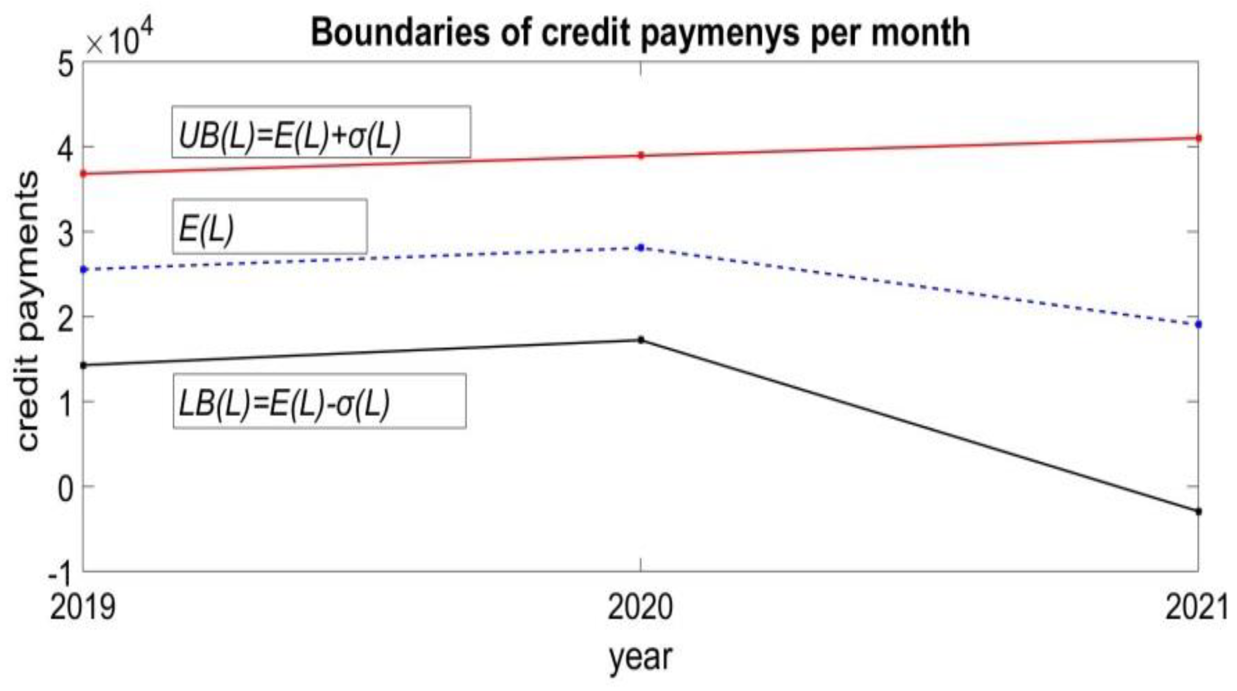
Estimation of average E(L) and $σ (L)$ for the previous historical period of credit payments. For the case of 2019 this gives $E_{2019} (L) = 25542$ and $σ_{2019} (L) = 11264$ .
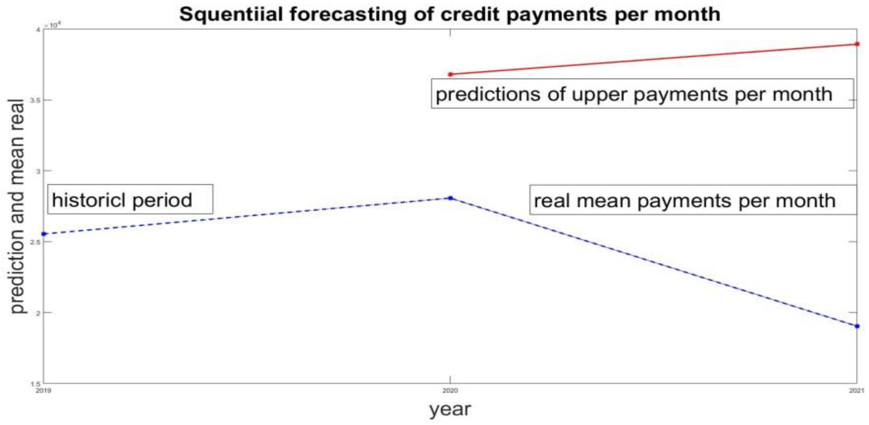
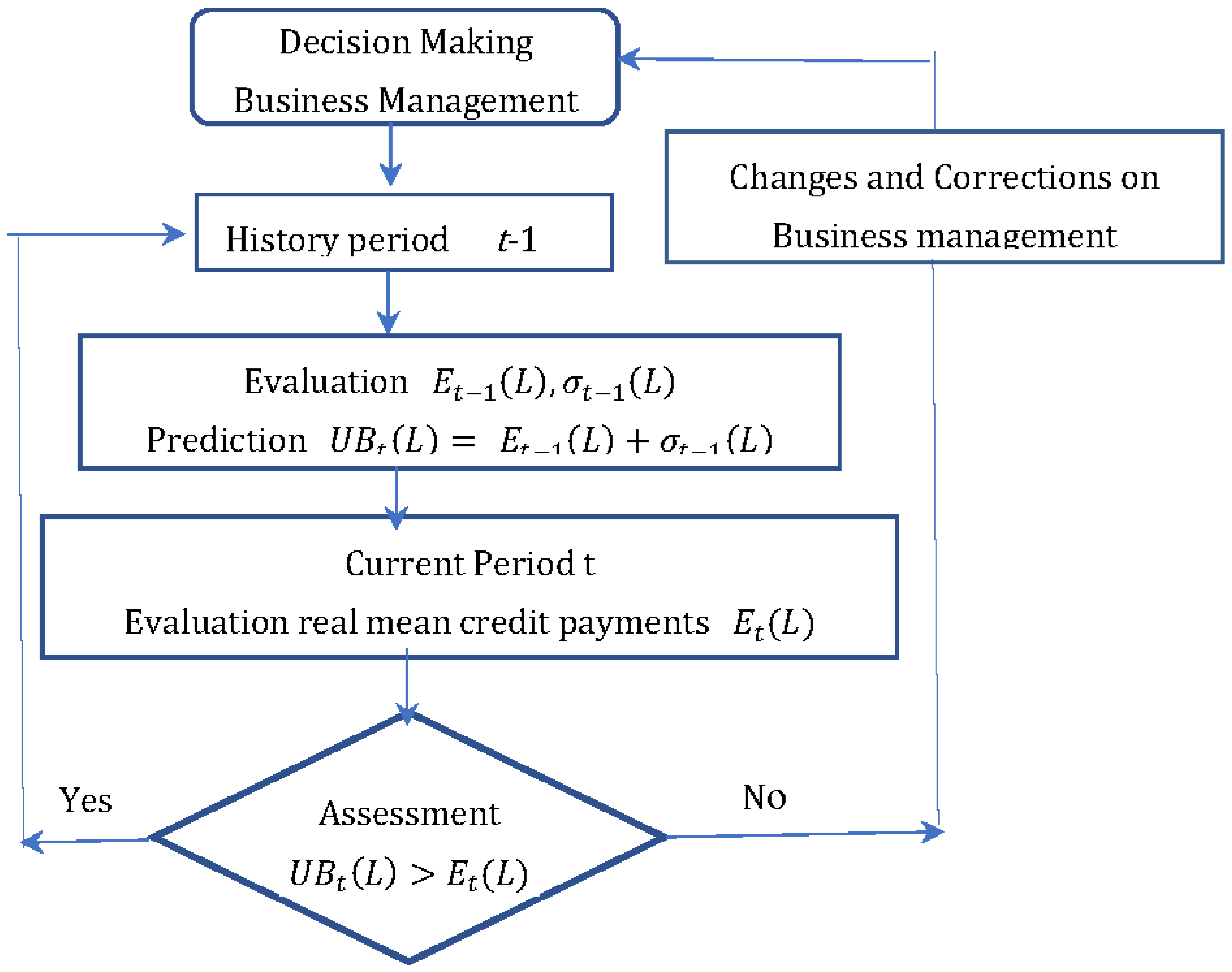
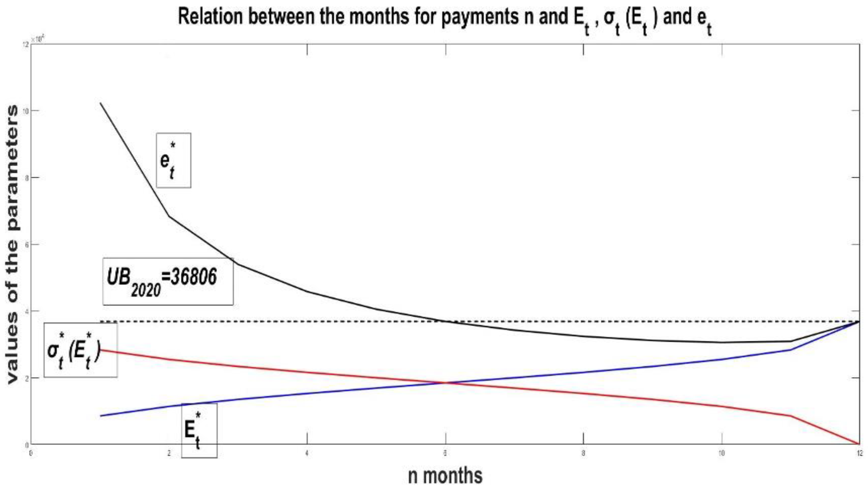
Estimate the upper bound $U B$ for this historical period. For the case of 2019 this gives ${U B}_{2019} (L) = 36806$ . The value of ${U B}_{2019} (L)$ is taken as the forecast of the monthly credit payments for 2020. Accordingly, this gives limits on the new credits that can be taken. This is the maximum amount of credit that can be used in 2020.
Evaluation of the forecast. At the end of 2020, average payments payments $E_{2020} (L)$ are estimated. It is a measure of the real values of credit payments L. The comparison between the forecast of the upper limit of the forecast volume of new credits ${U B}_{2019} (L)$ and the actual average payments $E_{2020} (L)$ gives the estimate

{{U B}_{2019} (L) > E}_{2020} (L) .

Thus, the prediction sets the upper bounds on future possible credit volumes L .

The application of this algorithm is applied with the data from Table 2 and Table 3 for the years 2019-2021. By successively moving the historical period forward by one year, we consistently obtain that the prediction inequality satisfies

{U B}_{t - 1} (L) > E_{t} (L),

where t is the reign year.

The results of using this management policy numerically are given in Table 4 and Figure 2

The applied sliding procedure makes forecasts and estimates for the needs of credit volumes that are recommended for livestock management in the current year. This assessment helps the decision makers decide on the need and/or eligibility to borrow additional resources through non-default funds. The prediction is based on previous business results, which indirectly takes into account the potential of the business entity to take credits or credits and successfully repay these financial obligations. The graphical interpretation of this predictive business management model is given in Figure 3.

The history period predicts the upper bound level of the credit payments. If these forecasts are lower than the actual average, the credit policy of the business management can be maintained in volumes. But if the average payments are higher than the predicted level, the management of the business must take measures to adjust and reduce the volumes of the credit policy.

This algorithm has been extended to be applied to a larger time horizon from monthly to annual time scale. This gives the total value of the possible credit volume that can be successfully be taken and recovered by the organization.

5. Assessment of the total credit volumes per year

In this case, the total amount of credit volume T is evaluated, according to the sum (1), where N and L are random variables. The estimation of annual values for mean

E_{12} (T)

and variance

{V a r}_{12} (T)

for 12 months is carried out by ratios (17) and (27), using

E_{12} (L)

E_{12} (N)

σ_{12} (L)

and

σ_{12} (N)

for the calculations data from Table 1. The estimated

E_{12} (T)

and

σ_{12} (T)

values are given in Table 5 for each year

Applying the algorithm of Section 4 with the sequence of values for

E_{12} (T)

and

σ_{12} (T)

gives the results presented in Table 6.

For this case of a forecast with a historical period longer than one year, the quantitative assessment of credit compliance is again the same

{U B}_{T - 1} (L) > E_{T} (L) .

Therefore, such a quantitative assessment can support the credit policy of the business entity for a longer time horizon.

6. Assessment of characteristics for individual credit

The initial data from Table 1 do not give the volume of the individual credits (i) that were taking per month. The available data refer to the total volume by month for both the credit volume

L

and their number

N

. Practical requirements require that the individual credit characteristics

E_{i}

and

σ_{i}

be evaluated. Such an estimate can be made in the same way by applying relations (17) and (27), but applied to the monthly scale. For this case, the values of the monthly parameters of credit payments are taken from Table 2, which are:

E_{1} (L) = 25 541

σ_{1} (L) = 1125

. The corresponding values for the mean monthly number are

E_{1} (N) = 2.67

and standard deviation

σ_{1} (N) = 0.78

Following (17), the average value of an individual credit payment can be estimated as

E_{1} (L) = E_{i} (L) E_{1} (N) or E_{i} (L) = \frac{E_{1} (L)}{E_{1} (N)} = \frac{25 541}{2.67} = 9578

The variance

V_{i} (L)

is evaluated from (27) or

σ_{1}^{2} = E_{1} (N) σ_{i}^{2} (L) + E_{i} (L) σ_{1}^{2} (L)

where

σ_{i} (L)

is unknown. Numerically, this gives

σ_{i} (L) = \sqrt{\frac{σ_{1}^{2} (L) - E_{i}^{2} (L) σ_{1}^{2} (N)}{E_{1} (N)}} = \frac{11264^{2} - 9578^{2} {0.78}^{2}}{25542} = 5170 .

The evaluation of the characteristics of an individual credit payment (i) per year is given in Table 7.

Application of the algorithm in Section 4 yields the “prediction-estimation” sequence with values from Table 8.

For this case of individual credit payment (i) the relation “prediction” > “actual mean” is again satisfied. Therefore, maintaining historical records of credit payments and applying ratios (17) and (27) the evaluated upper limit for potential credit remains lower compared to the actual average values of credit resources used,

{U B}_{T - 1} (l_{i}) > E_{T} (l_{i}) .

7. Potential solution for business management correction

The sequential credit limit prediction algorithm, given in Figure 3 omits a possible branch content recommendation when the upper limit and average payment criteria are not satisfied. Analytically, using the formal definition of upper bounds UB() from (30), the inequality leads to the form

{U B}_{t - 1} (L) < E_{t} (L) + σ_{t} (L)

(31)

In this case, changes and adjustments in the business management of the credit policy are required to reduce the total payments on the credits. In this section, a quantitative decision to make such a decision is motivated with appropriate formal descriptions. Changing the sign of the inequality in (31) can be done by reducing one or both components

E_{t} (L) a n d / o r σ_{t} (L) .

Our particular solution relates to monthly credit payments that are marked by

e_{t}

. These monthly payments are made only in n number of months, since the income of the farm does not have a regular inflow. Average credit payments per month on an annual basis are denoted as

E_{t}

. We need to define those values of

E_{t}

e_{t}

and

σ_{t}

respectively, which will satisfy the target relation

{U B}_{t - 1} \geq E_{t} (L) + σ_{t} (L)

(32)

with a predetermined number of n monthly payments. For such a defined credit payment policy, the credit payment variance will be as per the formal definition

σ_{t}^{2} = \frac{1}{12} [n (e_{t} - E_{t})^{2} + (12 - n)]

(32)

It is assumed that n-month credit payments will be made at a value

e_{t}

and no payments will be made the other months of the year. After rearranging (32) it follows

σ_{t}^{2} = \frac{1}{12} [n e_{t}^{2} - 2 n e_{t} E_{t} + 12 E_{t}^{2}] .

(33)

Our business policy is defined in such a way as to estimate that value of average monthly credit payments

E_{t}

that minimizes the variation of credit payments

σ_{t}^{2}

or the ratio

σ_{t}^{2} (E_{t})

from (33). The first derivative of this relation gives

\frac{d (σ_{t}^{2})}{d (E_{t})} = \frac{1}{12} (- 2 n e_{t} + 24 E_{t} = 0

which gives the solutions

E_{t}^{*} = \frac{n}{12} e_{t} or e_{t}^{*} = \frac{12 E_{t}}{n} .

(34)

Substituting the solutions (34) into the variance (33) gives its corresponding value

σ_{t}^{* 2} (E_{t}^{*}) = E_{t}^{* 2} (\frac{12}{n} - 1) = e_{t}^{* 2} \frac{n}{12} (1 - \frac{n}{12}) .

(35)

Relations (34) and (35) depend on the defined parameter n. The graphical interpretation of

E_{t}^{*} (n)

and

σ_{t}^{* 2} (n)

is given in Figure 4. The value of

E_{t}^{*}

depends linearly on n according to (34). But

σ_{t}^{* 2} (n)

is a nonlinear function towards n. The relationship

E_{t}^{*} (σ_{t}^{* 2} (n))

is plotted in Figure 4.

It can be seen that for different values of

E_{t}^{*}

the volatility

σ_{t}^{* 2}

has the same values. That is why, it is recommended to use only half of the graph

E_{t}^{*} (σ_{t}^{* 2} (n))

, which will give the appropriate values of the required credit. From a practical point of view, the larger value of the low-volatility credit is preferable, which corresponds to the upper part of the

E_{t}^{*} (σ_{t}^{* 2} (n))

curve.

The values of

E_{t}^{*}

and

σ_{t}^{*} (E_{t}^{*})

are found from the basic relation (32). For the specific case is valid

{U B}_{t - 1} \geq E_{t}^{*} + σ_{t}^{* 2} (E_{t}^{*}) = E_{t}^{*} + \sqrt{E_{t}^{* 2} (\frac{12}{n} - 1)},

where relation (35) is used for the analytical description of

σ_{t}^{* 2} (E_{t}^{*})

After rearrangements follows

E_{t}^{*} \leq \frac{{U B}_{t - 1}}{1 + \sqrt{(\frac{12}{n} - 1)}} .

(36)

The corresponding value of the standard deviation

σ_{t}^{*} (E_{t}^{*})

is evaluated according to (35) or

σ_{t}^{*} (E_{t}^{*}) \leq \frac{{U B}_{t - 1}}{1 + \sqrt{(\frac{12}{n} - 1)}} \sqrt{(\frac{12}{n} - 1)}

(37)

Accordingly, each of the n monthly payments

e_{t}

has a value according to (34) as

e_{t}^{*} \leq \frac{12}{n} (\frac{{U B}_{t - 1}}{1 + \sqrt{(\frac{12}{n} - 1)}} .

(38)

Relations (36)-(37) apply to the case of real monthly payments given with their mean and variance values from Table 2. Figure 5 shows the relationships between the number of months n , which determine how many months credit payments will be made in a year. The value of n is the argument of the mean credit payment per month

E_{t}^{*}

, the standard deviation

σ_{t}^{*}

and the value of the actual credit payment

e_{t}^{*}

for each month of category n. Calculations are performed for maximum level

{U B}_{2020} = 36806

. Equations (34) and (35) were used to evaluate these credit payment parameters.

The graphics present the internal relationships of the parameters

E_{t}^{*}

σ_{t}^{*} (E_{t}^{*})

and

e_{t}^{*}

from the number of months n when credit payments are due. For the case when the upper UB is a constant, as n changes, the real payment

e_{t}^{*}

for the month of category n decreases. The same is the case for the value of the standard deviation

σ_{t}^{*} (E_{t}^{*})

. Since the upper bound UB contains the sum of

E_{t}^{*} + σ_{t}^{*} (E_{t}^{*})

, as

σ_{t}^{*} (E_{t}^{*})

decreases, the corresponding values of

E_{t}^{*}

increase, which means that business can take larger credits. But relations (36)-(37) are inequalities and this gives that the graphs illustrate upper bounds for each parameter. An important feature of the graph

e_{t}^{*} (n)

says that there is a minimum below which the real monthly payment of category n can be found,

e_{t}^{*} (n)

. For the described case it is n=11. Therefore, if 11 months of the year credit payments are made, the monthly value will be the smallest. For the case illustrated here, n=11 and the monthly payment is

e_{t}^{*} (11)

= 3085.

8. Discussions

This research applies formal approaches to evaluate the statistical parameters of the sum of random values of credit payments and their random number. These relations were applied to estimate average monthly credit payments and total annual payments. Corresponding standard deviations are also estimated. This allows determining the upper and lower bounds of the actually required amount of credits. An algorithm is derived based on empirical results from real data from livestock management. The algorithm applies a sequential sliding procedure where historical data are used to predict future upper limits of credit volumes. Empirical results prove that the forecast levels are higher than the actual average volume of credit payments. The algorithm can be modified by extending or shortening the historical period. Extending the period will give numerical assessment of slow changes in market behavior and can support decision-making in a long period of time management. Conversely, shortening the historical period will benefit day-to-day operational management. This research does not directly link the results obtained to the exact recommendations for business management. However, its overall result is that it quantifies a really important part of business management, the amount of credit a business can afford. In addition, a quantitative solution is derived to minimize average credit payments, which is applicable if current credit payments are higher than the recommended upper level. This assessment is based on historical credit repayments, which indirectly reflect the entity’s potential to repay credits without default.

9. Conclusions

The paper derives a quantitative approach for assessment the characteristics of the credit policy of a business entity. Quantification was performed using conditional probabilistic relations for normal stochastic processes. The assessment of the credit policy of payment of an economic entity was carried out with available real data from the accounting book of animal husbandry. Numerical evaluations are made with the application of a derived algorithm, which performs the identification of the upper level of the permissible credit volumes and the consistent verification of the real average credit payments. A credit management solution based on the quantification and restricting the upper levels of credit payments is derived. A potential solution for business management by minimizing average credit payments is derived. Empirical results from the application of this algorithm provide useful links and support the quantification of credit policy for business management. This research can be expected to be extended in relation to the assessment of credit characteristics with managerial decisions to increase business profit and/or reduce credit risk while avoiding defaults. In this way, the current state of the business can be taken into account for taking a higher or lower value of credits necessary for the normal functioning of the business entity.

Acknowledgments

The research leading to these results has received funding from the Ministry of education and science under the National science program INTELLIGENT ANIMAL HUSBANDRY, grant agreement N Д01-62/18.03.2021.

Conflicts of Interest

The authors declare no conflict of interest.

References

Kipronoh, P.; Mweta, T. Overview of Working Capital Management: Effective Measures in Managing Working Capital Components to Entrepreneurs. European Journal of Business and Management, 2018, 10(8), 83-86. Available online: https://www.researchgate.net/publication/327435910_Overview_of_Working_Capital_Management_Effective_Measures_in_Managing_Working_Capital_Components_to_Entrepreneurs (Accessed on 09.12.2023).
Tiwary, D.; Paul S. Role of Bank Credit and External Commercial Borrowings in Working Capital Financing: Evidence from Indian Manufacturing Firms. Journal of Risk and Financial Management, 2023, 16(11) 468. Available online: https://www.mdpi.com/1911-8074/16/11/468 (Accessed on 09.12.2023). [CrossRef]
Ismail, R. Working Capital – An Effective Business Management Tool. International Journal of Humanities and Social Science Invention, 2017, 6(3), 12-23. Available online: https://www.researchgate.net/publication/315445011_Working_Capital_-_An_Effective_Business_Management_Tool (Accessed on 09.12.2023).
Pakdel, M.; Ashrafi, M. Relationship between Working Capital Management and the Performance of Firm in Different Business Cycles. Dutch Journal of Finance and Management, 2019, 3(1), 1-7. Available online: https://www.djfm-journal.com/article/relationship-between-working-capital-management-and-the-performance-of-firm-in-different-business-5874 (Accessed on 09.12.2023). [CrossRef]
Samithamby, S. Working Capital Management. SSRN Electronic Journal, 2020, 1-22. 10.2139/ssrn.3578141. Available online: https://papers.ssrn.com/sol3/papers.cfm?abstract_id=3578141 (Accessed on 09.12.2023). http://dx.doi.org/10.2139/ssrn.3578141.
Fatema, H.; Feysal, M.; Nobanee, H. Working Capital Management of Johnson and Johnson, 2022. Available online: https://www.researchgate.net/publication/358021457_Working_Capital_Management_of_Johnson_and_Johnson (Accessed on 11.12.2023).
Herdinata, C. Credit Policy Planning in Medium Scale Business. Mediterranean Journal of Social Sciences, 2017 8(1), 14-19. Available online: https://www.researchgate.net/publication/313786341_Credit_Policy_Planning_in_Medium_Scale_Business (Accessed on 11.12.2023). [CrossRef]
Reyad H.M.; Zariyawati M.A.; Ong T.S.; Muhamad H. The Impact of Macroeconomic Risk Factors, the Adoption of Financial Derivatives on Working Capital Management, and Firm Performance. Sustainability. 2022, 14(21), 14447. Available online: https://www.mdpi.com/2071-1050/14/21/14447 (Accessed on 11.12.2023). [CrossRef]
Ntiamoah, E. B.; Egyiri, P. O.; Fiaklou, D.; Kwamega, M. An Assessment of Credit Management Practices on Loan Performance. International Journal of Marketing, Strategy, Operations Research and Organizational Behavior, 2014, 30(20), 1127-1131, Available online: https://www.academia.edu/7871974/An_Assessment_of_Credit_Management_Practices_on_Loan_Performance?email_work_card=view-paper (Accessed on 11.12.2023).
Liu, Wenjuan. Enterprise Credit Risk Management Using Multicriteria Decision-Making. J. Mathematical Problems in Engineering, 2021, 1-10. Available online: https://www.hindawi.com/journals/mpe/2021/6191167/ (Accessed on 11.12.2023). [CrossRef]
Rutkowski, M.; Tarca, S. Regulatory Capital Modelling for Credit Risk. International Journal of Theoretical and Applied Finance, 2015, 18(5). Available online: https://www.worldscientific.com/doi/abs/10.1142/S021902491550034X (Accessed on 11.12.2023). [CrossRef]
Madaan, M.; Kumar, A.; Keshri, C.; Jain, R.; Nagrath, P. Loan default prediction using decision trees and random forest: A comparative study. IOP Conf. Series: Materials Science and Engineering, 2021, 1022 012042, IOP Publishing. Available online: https://iopscience.iop.org/article/10.1088/1757-899X/1022/1/012042 (Accessed on 12.12.2023). [CrossRef]
Bhanu, L. U.; Narayana, S. Customer Loan Prediction Using Supervised Learning Technique. International Journal of Scientific and Research Publications (IJSRP), 2021 11(6), 403-407. Available online: https://www.ijsrp.org/research-paper-0621/ijsrp-p11453.pdf (Accessed on 12.12.2023). [CrossRef]
Kumari, S.; Swapnesh, D.; Nayak, D. S. K.; Tripti, S. Loan eligibility prediction using machine learning: a comparative approach. Global Journal of Modeling and Intelligent Computing, 2023, 3(1), 48-54, ISSN: 2767-1917, Available online: https://www.researchgate.net/publication/372656643_LOAN_ELIGIBILITY_PREDICTION_USING_MACHINE_LEARNING_A_COMPARATIVE_APPROACH (Accessed on 12.12.2023).
Wu, W. Machine Learning Approaches to Predict Loan Default. J. Intelligent Information Management, 2022, 14, 157-164. Available online: https://www.scirp.org/pdf/iim_2022092709434339.pdf (Accessed on 12.12.2023). [CrossRef]
Aslam, U.; Aziz, H. I. T.; Sohail, A.; Batcha, N.K. An Empirical Study on Loan Default Prediction Models. Journal of Computational and Theoretical Nanoscience, 2019, 16(8), 3483-3488. Available online: https://www.researchgate.net/publication/335966806_An_Empirical_Study_on_Loan_Default_Prediction_Models (Accessed on 12.12.2023). [CrossRef]
Zhu, L.; Qiu, D.; Ergu,D.; Ying, C.; Liu, K. A study on predicting loan default based on the random forest algorithm, Procedia Computer Science, 2019, 162, 503-513, ISSN 1877-0509 Available online: https://www.sciencedirect.com/science/article/pii/S1877050919320277 (Accessed on 12.12.2023). [CrossRef]
Nalawade, S.; Andhe, S.; Parab, S.; Sankhe, A. Loan Approval Prediction. International Research Journal of Engineering and Technology, 2022, 09(04), 669-673, ISSN: 2395 Available online: https://www.academia.edu/85429526/Loan_Approval_Prediction?email_work_card=view-paper (Accessed on 12.12.2023).
Orlova, E. Mechanism and Model for Decision-Making in Credit Risk Management. Conference: Proceedings of the Fourth Workshop on Computer Modelling in Decision Making (CMDM 2019), 2019. Available online: https://www.atlantis-press.com/proceedings/cmdm-19/125925611 (Accessed on 12.12.2023). [CrossRef]
Olabamiji, O.; Michael, O. Credit Management Practices and Bank Performance: Evidence from First Bank. South Asian Journal of Social Studies and Economics, 2018, 1(1), 1-10. Available online: https://journalsajsse.com/index.php/SAJSSE/article/view/502 (Accessed on 12.12.2023). [CrossRef]
Mburu, I.; Mwangi, L.; Muathe, S. Credit Management Practices and Loan Performance: Empirical Evidence from Commercial Banks in Kenya. International Journal of Current Aspects in Finance, Banking and Accounting, 2020, 2(1), 51-63. ISSN 2707-8035 Available online: https://journals.ijcab.org/journals/index.php/IJCFA/article/view/105 (Accessed on 12.12.2023). [CrossRef]
Herdinata, C. Credit Policy Planning in Medium Scale Business. Mediterranean Journal of Social Sciences, 2017, 8(1), 14-19. Available online: https://dspace.uc.ac.id/bitstream/handle/123456789/961/Paper961.pdf?sequence=6&isAllowed=y (Accessed on 14.12.2023). [CrossRef]
Farhan, N.H.S.; Almaqtari, F.A.; Al-Matari, E.M.; SENAN, N.A.M.; Alahdal, W.M.; Hazaea S.A. Working Capital Management Policies in Indian Listed Firms: A State-Wise Analysis, Sustainability, 2021, 13(8), 4516. Available online: https://www.mdpi.com/2071-1050/13/8/4516 (Accessed on 14.12.2023). [CrossRef]
Olabisi, J.; Oladejo, D. A.; Adegoke, J. F.; Abioro, M. Credit management policy and firms’ profitability: evidence from infant manufacturing firms in southwest Nigeria. The Journal Contemporary Economy, 2019, 4(4), 59-69, ISSN 2537–4222. Available online: https://www.researchgate.net/publication/338423067_CREDIT_MANAGEMENT_POLICY_AND_FIRMS'_PROFITABILITY_EVIDENCE_FROM_INFANT_MANUFACTURING_FIRMS_IN_SOUTHWEST_NIGERIA (Accessed on 14.12.2023).
Otto, W. Management of trade credit by small and medium-sized enterprises. Journal of Economic and Financial Sciences, 2018, 11(1), 1-8. Available online: https://www.researchgate.net/publication/324361630_Management_of_trade_credit_by_small_and_medium-sized_enterprises (Accessed on 14.12.2023). [CrossRef]
Poot, M. Credit and Collection Management Practices, Credit Risk Management, and Financial Performance of Private Higher Educational Institutions (HEIs) in the Philippines: Basis for Continuous Improvement. Proceedings of the 8th International Conference on Entrepreneurship and Business Management (ICEBM 2019), Advances in Economics, Business and Management Research, 2020, 14, 288-295. Available online: https://www.researchgate.net/publication/342778867_Credit_and_Collection_Management_Practices_Credit_Risk_Management_and_Financial_Performance_of_Private_Higher_Educational_Institutions_HEIs_in_the_Philippines_Basis_for_Continuous_Improvement (Accessed on 14.12.2023). [CrossRef]
Kipronoh, P.; Mweta, T. Overview of Working Capital Management: Effective Measures in Managing Working Capital Components to Entrepreneurs. European Journal of Business and Management, 2018, 10(8), 83-86, ISSN 2222-1905, Available online: https://www.researchgate.net/publication/327435910_Overview_of_Working_Capital_Management_Effective_Measures_in_Managing_Working_Capital_Components_to_Entrepreneurs (Accessed on 14.12.2023).
Zimon, G. Working Capital. Encyclopedia, 2021, 1(3), 764-772. Available online: https://www.mdpi.com/2673-8392/1/3/58 (Accessed on 14.12.2023). [CrossRef]
Pakdel, M.; Ashrafi, M. Relationship between Working Capital Management and the Performance of Firm in Different Business Cycles. Dutch Journal of Finance and Management, 2019, 3(1), 1-7. Available online: https://www.researchgate.net/publication/335204064_Relationship_between_Working_Capital_Management_and_the_Performance_of_Firm_in_Different_Business_Cycles (Accessed on 14.12.2023). [CrossRef]
Demiraj, R.; Dsouza, S.; Abiad, M. Working Capital Management Impact on Profitability: Pre-Pandemic and Pandemic Evidence from the European Automotive Industry. Risks, 2022, 10(12):236. Available online: https://www.mdpi.com/2227-9091/10/12/236 (Accessed on 14.12.2023). [CrossRef]
Ngugi, D. Quantitative Methods For Business Management. 2018; p. 420. Available online: https://www.researchgate.net/publication/329031752_Quantitative_Methods_For_Business_Management (Accessed on 14.12.2023).
Lariviere, M. A.; Porteus, E.L. Stalking information: Bayesian inventory management with unobserved lost sales. Management Science, 1999, 45(3), 346–363. Available online: https://pubsonline.informs.org/doi/10.1287/mnsc.45.3.346 (Accessed on 14.12.2023). [CrossRef]
Standard Normal Distribution Showing Standard Deviations. Digital image. Statistics How To, 2016. Available online: https://www.statisticshowto.com/probability-and-statistics/ (Accessed on 14.12.2023).

Figure 1. Graphical representation of the limits of the monthly volumes of credit payments E(L).

Figure 2. Estimates between predicted and actual averages.

Figure 3. An algorithm for sequential credit limit prediction.

Figure 4. Graphic representation of the relation

E_{t}^{*} (σ_{t}^{* 2} (n))

Figure 4. Graphic representation of the relation

E_{t}^{*} (σ_{t}^{* 2} (n))

Figure 5. Ratio between months for payments and

E_{t}^{*}

σ_{t}^{*} (E_{t}^{*})

and

e_{t}^{*}

Figure 5. Ratio between months for payments and

E_{t}^{*}

σ_{t}^{*} (E_{t}^{*})

and

e_{t}^{*}

Table 1. Initial data for credits per month.

Month	2019 l_i [BGN]	2019 n_i [BGN]	2020 l_i [BGN]	2020 n_i [BGN]	2021 l_i [BGN]	2021 n_i [BGN]
I	7690	1	45802	3	4750	1
II	6000	1	34297	2	19523	4
III	25195	3	11505	1	18447	4
IV	25195	3	45802	5	20598	6
V	25195	3	22463	3	0	0
VI	25195	3	22463	3	0	0
VII	25195	3	22463	3	58569	4
VIII	25195	3	38614	5	14824	3
IX	25195	3	26665	4	0	0
X	25195	3	27760	5	19824	4
XI	45802	3	19523	5	0	0
XII	45802	3	19523	3	63315	6

Table 2. Statistical parameters of random L and N per month.

Year	$E (L)$	σ(L)	$E (N)$	σ(N)
2019	25542	11264	2.67	0.78
2020	28074	10853	3.5	1.31
2021	19041	21965	2.67	2.35

Table 3. Limits on the real values of L and N.

Year	min $L B (L) = E (L) - σ (L)$	max $U B (L) = E (L) + σ (L)$	min $E (N) - σ (N)$	max $E (N) - σ (N)$
2019	14278	36806	1.89	3.45
2020	17221	38927	2.19	4.81
2021	-2924	41006	0.35	5.02

Table 4. Numerical data for the consistent forecasting of credit volumes for a month and the average value of actual credit payments.

Historical period	Prediction of maximal credit for 2020	Real mean value of payments 2020	Historical period	Prediction of maximal credit for 2021	Real mean value of payments 2021
2019	36 806	28 074	2020	38 027	19 041

Table 5. Estimated statistical parameters to the total volume T per year.

Year	2019	2020	2021
$E_{12} (T)$	306 510	336 880	228 497
$σ_{12} (T)$	39 021	37 596	76 089
${U B}_{12} (T) = = E_{12} (T) + σ_{12} (T)$	345 531	374 476	304 586

Table 6. Numerical data on the consistent forecasting of credit volumes for a year.

Historical period	2020 maximum credit forecast	Real average payments 2020	Historical period	2021 maximum credit forecast	Real average payments 2021
2019	345 531	336 880	2020	374 476	228 497

Table 7. Evaluated statistical parameters for individual credit (i) per year.

Year	2019	2020	2021
$E_{i} (L)$	9578	8021	7140
$σ_{i} (L)$	5170	1379	8687
${U B}_{i} = = {E_{i} (L) + σ}_{i} (L)$	14 748	9400	15 828

Table 8. Numerical data on the sequential forecasting of individual credit volume (i).

Historical period	2020 maximum credit forecast	Real average payments 2020	Historical period	2021 maximum credit forecast	Real average payments 2021
2019	14 748	8021	2020	9400	7140

Disclaimer/Publisher’s Note: The statements, opinions and data contained in all publications are solely those of the individual author(s) and contributor(s) and not of MDPI and/or the editor(s). MDPI and/or the editor(s) disclaim responsibility for any injury to people or property resulting from any ideas, methods, instructions or products referred to in the content.

© 2023 by the authors. Licensee MDPI, Basel, Switzerland. This article is an open access article distributed under the terms and conditions of the Creative Commons Attribution (CC BY) license (http://creativecommons.org/licenses/by/4.0/).

Copyright: This open access article is published under a Creative Commons CC BY 4.0 license, which permit the free download, distribution, and reuse, provided that the author and preprint are cited in any reuse.

MDPI Initiatives

Important Links

Choose an area of interest and we will send you notifications of new preprints at your preferred frequency.

Disclaimer

Quantitative Planning Credit Policy for Business Management

Abstract

1. Introduction

2. Review of credit management policies

3. Formal modeling of the credit business model

4. Analysis of the farm’s credit policy

5. Assessment of the total credit volumes per year

6. Assessment of characteristics for individual credit

7. Potential solution for business management correction

8. Discussions

9. Conclusions

Acknowledgments

Conflicts of Interest

References

MDPI Initiatives

Important Links

Subscribe