1. Introduction
Peanut, also known as groundnut (
Arachis hypogaea L.) is a major economically important legumes and crucial source of protein and vegetable oil, which is widely grown in more than 100 countries in the world, especially in China, India, Nigeria, and the United States [
1]. Early leaf spot (
Cercospora arachidicola S. Hori) and late leaf spot (
Cercosporidium personatum) are the most destructive foliar diseases of peanut in the late growth stage and commonly result in necrotic lesions on leaves, stems, and become a dominant yield-limiting factor of peanut worldwide. Defoliation occurs shortly after the appearance of leaf lesions, and if not controlled, can reach 100% and yield losses of up to 70% [
2]. The visual investigation in the field usually is the most common and traditional way to acquire the peanut leaf spot disease infection information. This method requires investigators mastering relevant expertise of plant protection and has the disadvantages of being highly subjective, time-consuming, and lagging behind proper spraying. Timely and accurate detection on peanut leaf spot disease is important to adequately accomplish disease management measures.
At present, fungicide spraying is a standard measure to control peanut leaf spot. However, the excessive use of fungicides enhances peanut disease management cost and causes problems such as environmental pollution and threats to food safety [
2]. Therefore, prevention and precision spraying according to the occurrence of diseases in the field can effectively cut economic losses, reduce fungicide application, and ensure food safety [
3].
Traditional methods of disease monitoring are based on manually covering large areas of farmland or plant communities at regular intervals (weekly or monthly), which can result in areas being inadequately monitored, thus missing early signs of plant disease. So traditional disease monitoring methods are limited by time and space[
4,
5]. In recent years, machine learning and deep learning methods have shown strong potential in the field of agriculture, especially in the task of plant disease prediction [
4,
5,
6,
7]. Azadbakht et al. [
8] analyzed to characterize the performance of leaf rust detection in wheat using four machine learning methods, namely, Gaussian process regression, Random Forest regression, v-support vector regression and boosted regression tree and the researchers also predicted the severity of rust disease. Some research has also been devoted to random forest approach to identify common characteristics of soil microbial communities to predict the potential of wilt [
9]. However, traditional machine learning models usually require manual feature engineering, i.e., selecting and designing appropriate features, which may require domain knowledge and experience, and may perform poorly when dealing with highly nonlinear and complex relational problems [
10,
11]. Deep learning, on the other hand, especially Recurrent Neural Networks (RNN) or Long Short-Term Memory Networks (LSTM), is able to automatically capture patterns and trends in time-series data [
12,
13]. It is worth mentioning that the combined use of machine learning and deep learning may achieve more satisfactory results. For example, deep learning models (e.g., convolutional neural networks) are used to extract advanced features from raw data, and then these features are used in traditional machine learning models (e.g., support vector machines, random forests) for prediction [
14,
15,
16].
A leading cause for the prevalence of plant diseases is weather conditions, in addition to pathogen spread as a major factor [
17,
18,
19]. Plant disease prediction models are usually trained based on a large amount of historical weather data and disease monitoring data. By analyzing these data through deep learning or machine learning, the models can learn the association between weather conditions and plant diseases, and thus make predictions about future disease outbreaks. A study reported the use of Aprioro algorithm to determine the association rules between meteorological factors and cotton pests and diseases, and proposed a time-series prediction model for cotton pests and diseases by LSTM [
20].
Long Short-Term Memory Network (LSTM) is a special type of Recurrent Neural Network (RNN) with excellent sequence modeling capability. Its ability to capture long-term dependencies in time series data makes LSTM perform well in time series prediction tasks [
21]. Although both Back-Propagation (BP) neural networks and Generalized Regression Neural Networks (GRNN) can be used for prediction model building, they are prone to the problem of gradient vanishing or gradient explosion when dealing with long sequences, have difficulty in capturing long-term dependencies, and lack a gating mechanism, which is not user-friendly when dealing with information flow in sequences. Therefore, this study aimed to accurately predict the occurrence of peanut leaf spot disease using CNN and LSTM models, combined with years of meteorological data and disease survey records.
In this study, we discarded the traditional feature correlation analysis and use multiple sets of meteorological features as model inputs to combat the loss of important hidden features. We also discarded the traditional convolutional neural network down-sampling process, and we utilized continuous multiple convolution and short-circuiting mechanisms connected with the Squeeze-and-Excitation attention mechanism together as the LSTM upstream input. By constructing an efficient prediction model, we predicted the outbreak of leaf spot disease in advance, which will help farmers to take appropriate control measures in time and minimize the adverse effects of the disease on peanut yield and quality.
2. Materials and Methods
2.1. Data Acquisition and Cleaning
Open-Meteo is an open-source weather API and offers free access for non-commercial use (
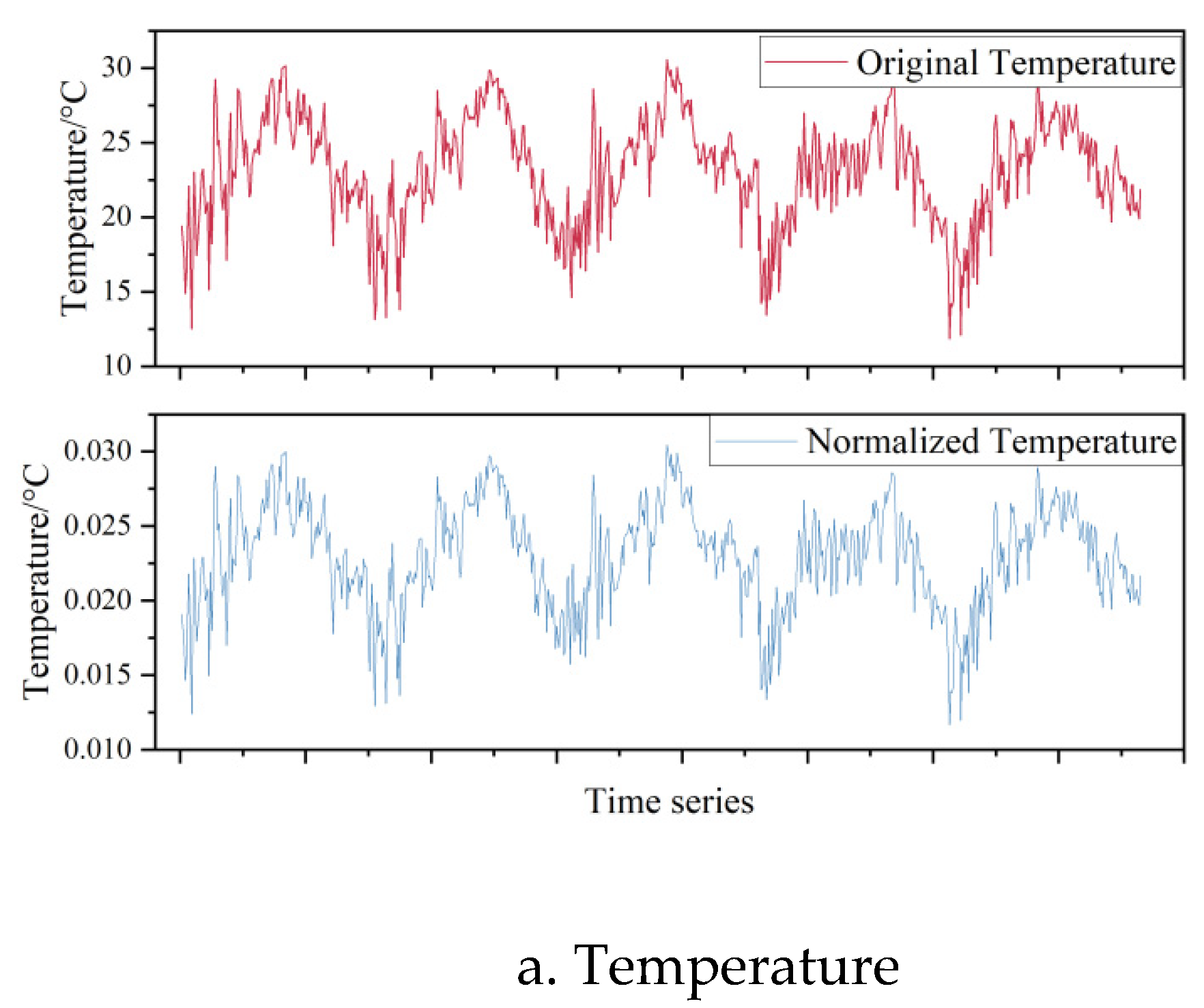
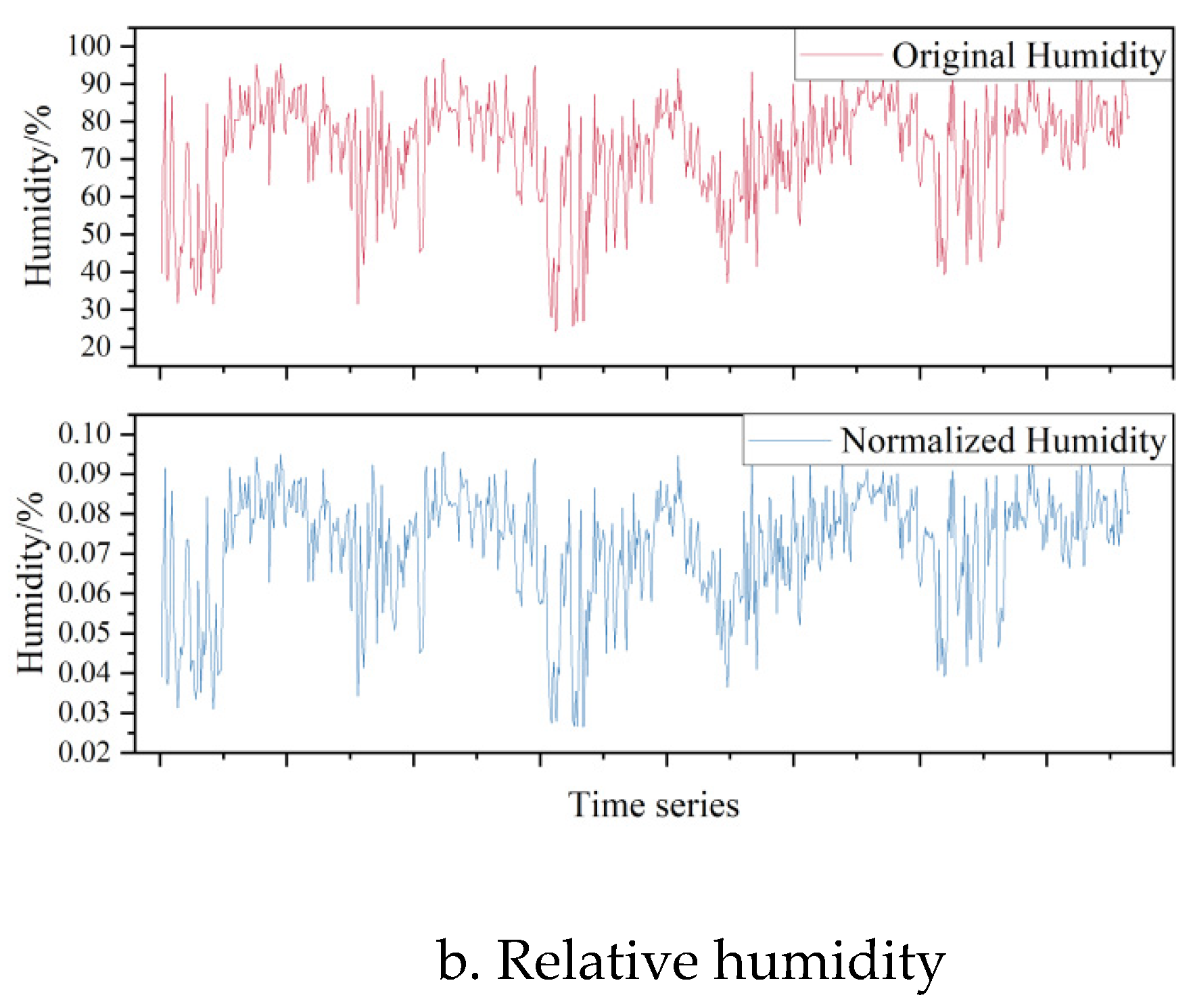
https://open-meteo.com/). We purchased from this website to obtain five consecutive years of meteorological data from 2017 to 2023 for the peanut planting base in Laixi, Qingdao City, Shandong Province, containing nine elements, including temperature, humidity, dew point, precipitation, sea level barometric pressure, surface barometric pressure, wind direction, wind speed, and solar radiation. Open-Meteo provides high-resolution open data from 1 to 11 kilometers, which is more reflective of the meteorological conditions over a large area. The monitoring range of a single weather station is very limited, which may be only a few tens of meters, so we calibrate the data through a small weather station at the experimental base. In this study, we used the data from 2017 to 2021 as inputs to the model, and the data from 2022 and 2023 as to conduct the actual validation of the model. Considering that if an input has a large scale, its weight update may be larger than other inputs, which may cause the model to rely too much on certain features during training. In order to eliminate the presence of scale effects between different metrics, the data are normalized. Normalization speeds up the convergence of the model while preventing numerical overflow and gradient explosion, and improves the accuracy of the prediction model to some extent. We use the mapminmax function to carry out the normalization operation of the data, and its calculation principle is:
The time series raw meteorological data and normalized data are shown in
Figure 1.
2.2. Disease survey
Peanut plants were cultivated in an experimental field at the Shandong Peanut Research Institute (SPRI) in Laixi city, Qingdao, China, which is located at latitude 36°48′46 "N - longitude 120°30'5 "E. The field has been planted biennially in a peanut/wheat/corn rotation. Peanuts are sown in early May each year, and the experimental site is a multi-year peanut cropping field with severe peanut leaf spot (brown spot and black spot). Peanut planting plots were arranged in randomized groups, repeated twice, and the density of peanut planting was 10,000 holes per mu, with two grains per hole. Peanut varieties are "HuaYu", "LuoHua", "PuHua" three series, which are moderate or highly susceptible to leaf spot disease. We use manual survey method to record the disease index and relative resistance index sampling, from the early July to the beginning of September each year for the survey. The severity of peanut leaf spot was assessed on a scale of 0-4, with 0 representing no disease and 4 representing plant death (
Table 1).
We randomly selected 20 plants in each plot to assess the severity of leaf spot disease. The average disease index (DI) was calculated using the following formula:
Due to the weather anomaly in 2017, peanut disease occurrence was generally light in June and July due to persistent high temperatures and drought, and the rest of the year did not experience weather anomalies. Based on manual surveys, peanut brown spot disease appeared in mid-July, peanut black spot disease appeared in mid- to late August, and with increased rainfall in mid- to late August, peanut black spot and brown spot disease occurred in large quantities, and net blotch disease basically did not occur.
2.3. Model building
2.3.1. Related work
LSTM is an optimized form of RNN designed to solve the problems of gradient vanishing and gradient explosion faced by traditional RNNs [
22]. Its structure contains an input layer, an implicit layer and an output layer. LSTM introduces specialized memory units and gating mechanisms to efficiently capture and retain long-term dependencies in sequential data.
CNN effectively reduces the number and dimensionality of deep neural network parameters while deeply mining spatial features of meteorological data through operations such as local connection, weight sharing and pooling operation, which makes the computational speed and data analysis ability of convolutional god network effectively improved. Its basic structure consists of input layer, convolutional layer, pooling layer, fully connected layer and output layer.
Among them, the convolutional layer performs convolutional computation on all input information, and at the same time, the data features are effectively extracted through the pooling layer to compress the input features, simplify the computational complexity of the network, and extract the main features, and the calculation method of convolution can be based on the formula (3):
where f_c is the activation function, n, m and k are the length, width and depth of the node matrix, respectively;
is the value of node (x, y, z) in the node matrix;
is the weight of the filter input node (x, y, z) with respect to the ith node in the unit matrix; and
is the bias parameter used to fit the weight data.
2.3.2. Squeeze-and-Excitation Networks Block
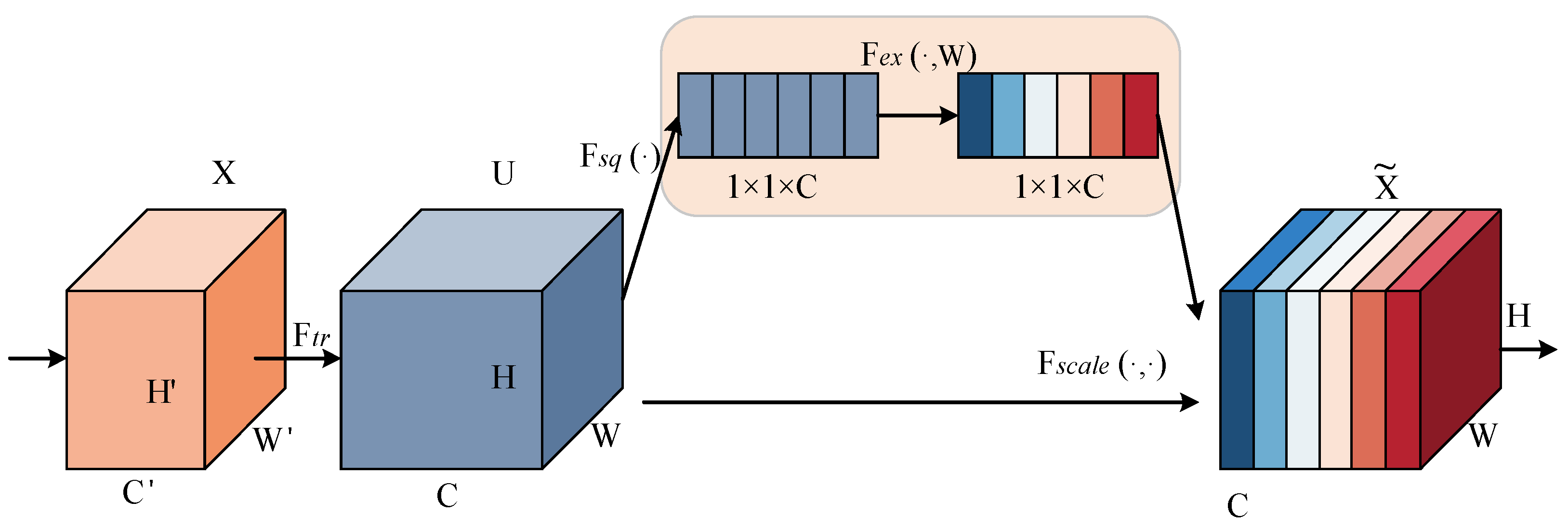
The traditional feature transfer method is to pass the weights such as the Feature Map of the network to the next layer, while the Squeeze-and-Excitation (SE) Networks Block attention mechanism adaptively re-corrects the intensity of the feature response between channels through the global loss function of the network, that is to say, the SE block is to extract effective features by augmenting or aligning the corresponding channels for different tasks through the weights of the importance of each feature channel [
23]. As shown in the
Figure 2, the process of an SE block is divided into two steps: Squeeze and Excitation. Squeeze obtains the global compressed feature vector of the current Feature Map by performing Global Average Pooling on the Feature Map layer, and Excitation obtains the weights of each channel in the Feature Map through the two-layer full connectivity, and uses the weighted Feature Map as the input of the next layer of the network. The weighted Feature Map is used as the input to the next layer of the network.
In the figure, the Feature Map is squeezed into a 1×1×C feature vector to get the global information embedding (feature vector) for each channel of U. This process is based on the global average pooling to obtain the average value of the Feature Map, i.e., Equation (3):
After Excitation learns the feature weights of each channel in C, the feature map with the same dimension as the squeeze operation is obtained, and the computation process is as follows:
where δ denotes the ReLU activation function, denotes the sigmoid activation function. W1 and W2 are the weight matrices of the two fully connected layers, respectively. r is the number of hidden nodes in the middle layer. The compressed and activated values will be weighted by Fscale(⋅,⋅) of U to get the feature map.
2.3.3. The proposed model
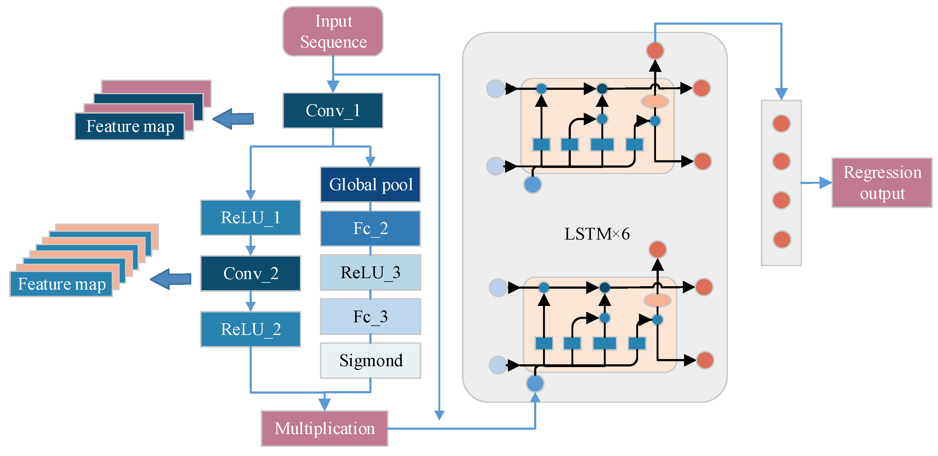
In the design of the improved model, since the dimension of the input features was not large, we designed the part of the CNN as a three-layer convolutional structure and fused the SE Attention Mechanism module through the short-circuit mechanism, and the Feature map after convolutional neural network was used as the input of the LSTM. The increase of the number of implicit layers of the LSTM helped to improve the prediction performance of the model, which, although increased the amount of computation, it didn't not affect the performance of the computer. Therefore we set the number of LSTM hidden units to 8.
As shown in
Figure 3, we preprocessed M × N sequences of historical meteorological data and condition indices and used them as input sequences for this model. In the CNN layer, we set the convolution kernel as 2 convolutional layers of 3×1 and the pooling kernel as 2 maximal pooling layers of 5×5. The activation function of the convolutional layer is ReLU function and the padding was set to the same. The pooling layer took the overall statistical features of the regions adjacent to a position of the input matrix as the output for that position, with the aim of reducing the number of nodes in the fully connected layer and thus simplifying the network parameters. The convolutional layer and the pooling layer together formed a feature extractor that can maximized the potential information of the input values to be reasonably extracted, and also reduced the bias that occurs when the data was extracted by human beings. Therefore, in this study, CNN was first used to extract features from the normalized data, and then analyzed and predicted by LSTM network. The data was extracted from the convolutional layer as well as the pooling layer and the jointly obtained feature map was fed into the LSTM layer of the neural network through the SE Attention Mechanism. The LSTM layer mainly learned the features extracted from the CNN layer. The model was built with 8 layers of hidden units to fully learn the extracted features.
When the data was input at moment t, the LSTM first went through the computation of the forgetting gate:
The value of the input gate was then passed:
The formula for the candidate memory cell was:
The current memory cell state value was:
Then the value of the output gate was:
So the final output of LSTM at moment t was:
In equations (2) to (7), σ represents the sigmond activation function, and tanh is the hyperbolic tangent activation function. 、、 are the values of the forgetting gate, the input gate and the output gate, respectively, and the weights of the forgetting gate, the input gate, the state gate, and the output gate are: 、、、 and the weights of the state gate and the output gate, respectively. weights and biases of the cell and output gates, respectively.
The training of neural networks was prone to overfitting, when overfitting occurs, even if the model showed a small loss function value and high accuracy in the training set, but when applied to the test set, not only the loss value was large, but also the prediction accuracy was low, and the model had no practical significance. Dropout randomly and temporarily set the neurons of the neural network to zero during the training process, that is, it "discarded" the output of these neurons. "Dropout" the output of these neurons. In this way, each time a forward propagation was performed, it was equivalent to training a different, smaller sub-network. This process was similar to randomly removing neurons during training, thus reducing the network overdependence on specific neurons. We therefore set 2 layers of Dropout (with the discard rate set to 0.3 and 0.5 respectively) to prevent overfitting during training.
The hardware device used for the model building process is a Dell laptop with Intel(R) Core(TM) CPU i5-8250U @1.60 GHz processor, 16GB of RAM, Window10 operating system, and the software for data processing and network training is MATLAB 2022b.
2.4. Evaluation metrics
Prediction performance evaluation indexes are criteria for evaluating the performance of peanut leaf spot disease index prediction models. In this study, the coefficient of determination (), mean absolute error (MAE), mean bias error (MBE) and root mean square error (RMSE) were used to evaluate the prediction accuracy of the disease prediction model.
reflects the degree of fit of the model, and the closer its value is to 1, the better the input explains the response, which is calculated as:
MAE is the mean of the absolute value error, which truly reflects the magnitude of the prediction error and is calculated as:
MBE reflects the average deviation between the predicted value and the true value. The indicator is directional, with positive values indicating overestimation and negative values indicating underestimation, and is calculated using the formula:
RMSE takes into account the variation of the actual value and measures the average magnitude of the error, calculated as:
In each of the above formulas
denotes the test value, the actual value of the output at that moment;
denotes the predicted value of the output through the model prediction; N is the number of samples in the test set; and
denotes the sample mean.
3. Results and analysis
3.1. Model Optimization
An exponential scale was used to set the learning rate during the training process, and comparative experiments with different learning rates and number of training parameters were conducted. A larger learning rate may cause the model to converge faster during training. However, if the learning rate was too large, it may cause the model to oscillate around the optimal point or even fail to converge. On the contrary, a smaller learning rate may lead to slower convergence or even fall into a local minimum and fail to continue learning. According to the results in
Table 2, it can be seen that under the same number of training times, when the learning rate was 0.001, the average accuracy of the improved network model on the test set was better than other values especially the R^2 reached 0.951. The MAE, MBE, and RMSE metrics we were concerned about had different degrees of decreased in comparison with the learning rate of 0.01. On the contrary, if the learning rate was set to 0.0001, even though the model can converge quickly, there was anomalous performance of the model
R2 with this hyperparameter.
For this study, we used multiple inputs to build the prediction model. Among the many meteorological metrics, such as dew point and precipitation data with rapidly changing gradients or the presence of noise, SGDM optimizers were less adaptive to non-stationary data, while adaptive learning algorithms (such as the Adam optimizer) are more advantageous. In other words, the adaptivity of Adam may be more advantageous for different input features when they may have different scales or importance. Moreover, Adam introduced the concept of momentum, which helped to accelerate convergence by considering an exponentially weighted moving average of the gradient to overcome local minima during training [
27,
28,
29]. This was useful for dealing with complex loss surfaces or avoiding falling into local minima.
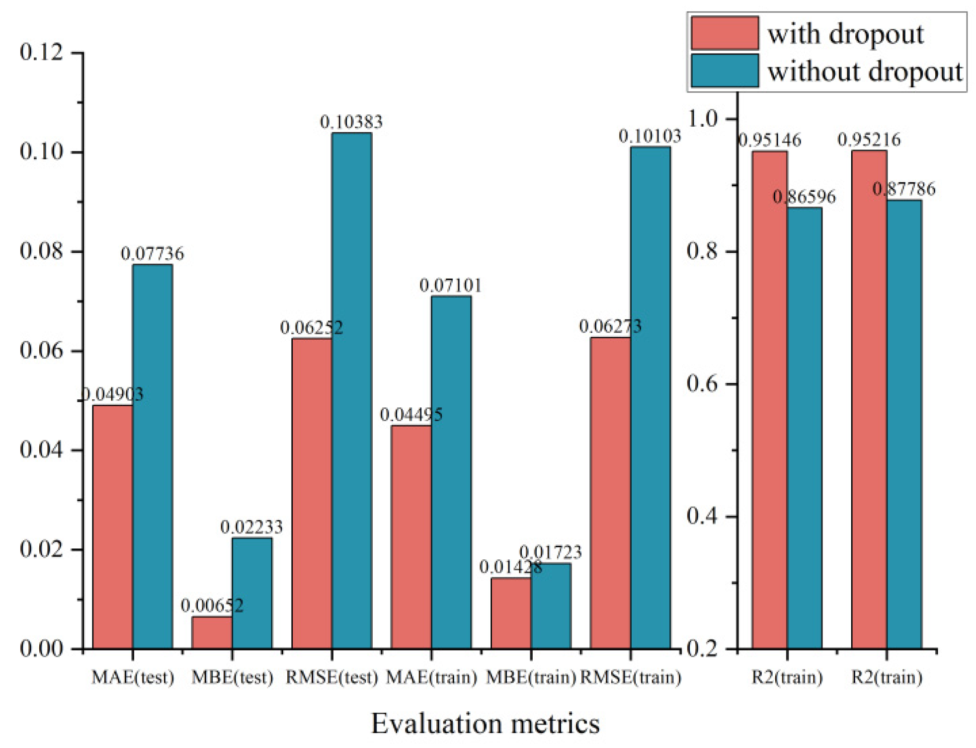
In addition, in order to reduce the interaction between LSTM hidden nodes and decrease the dependence on local features, we added dropout when designing the network, and it is obvious that the addition of dropout decreased the test data by 0.028, 0.016, and 0.041 in MAE, MBE, and RMSE, respectively, and improved the
by 0.0855 as shown in
Figure 4.
3.2. Disease Index Prediction
We constructed the weather data containing nine elements and the disease index and disease warning time as a dataset (weather data as input, disease index and disease warning time as output), and divided it into the training set, testing set and validation set according to the ratio of 7:2:1 in the hold-out method [
24]. After the training of the improved network, we got the prediction results on the training set and test set, respectively.
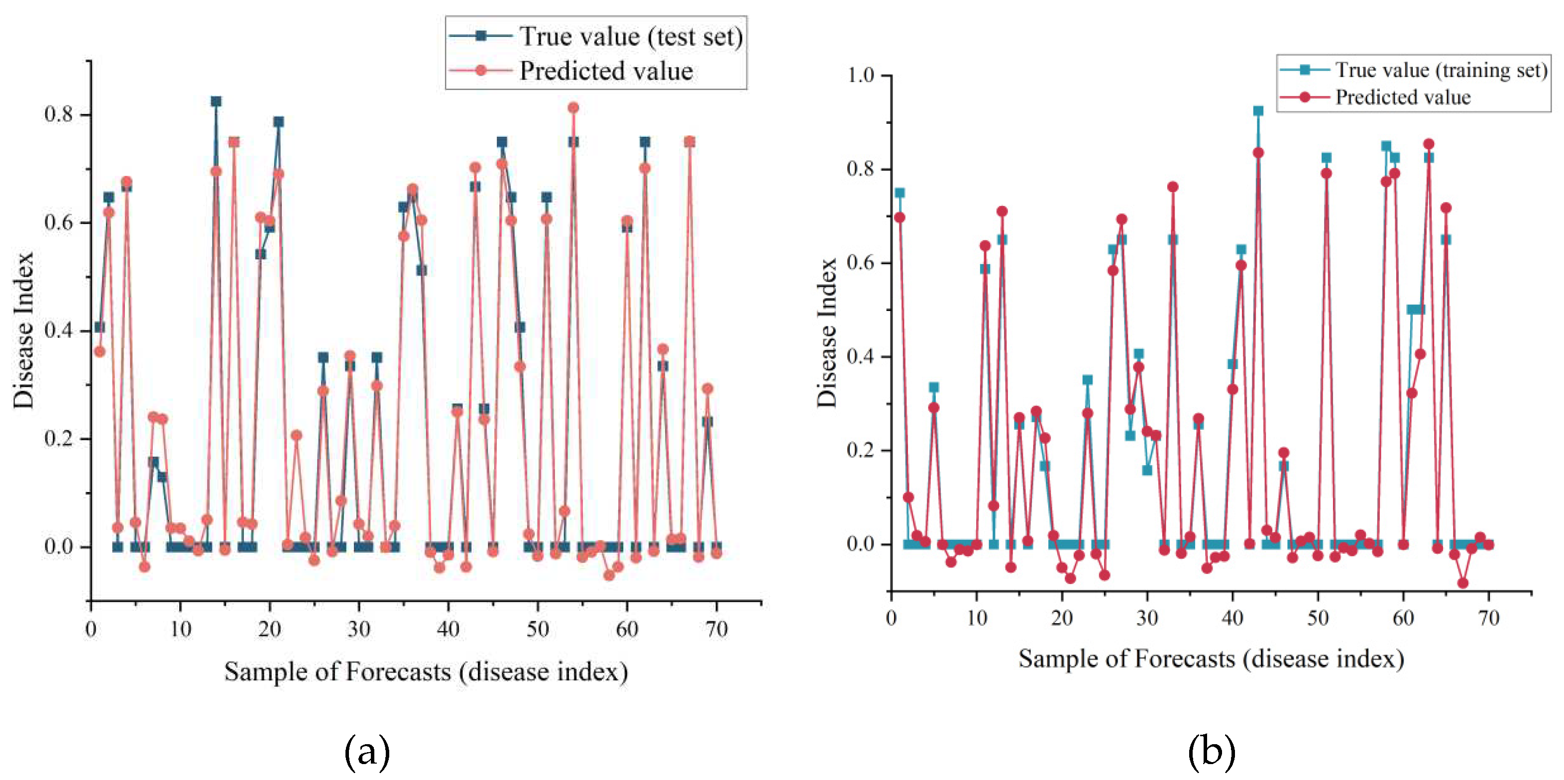
For disease index prediction, we observed that the model achieved disease index prediction with randomly disrupted samples. In
Figure 5b, the prediction performance of the model for the test set data was subsequently not as good as that of the training set data in
Figure 5a, but overall, the true and predicted values matched well, and there was no overfitting such as poor accuracy on the test set.
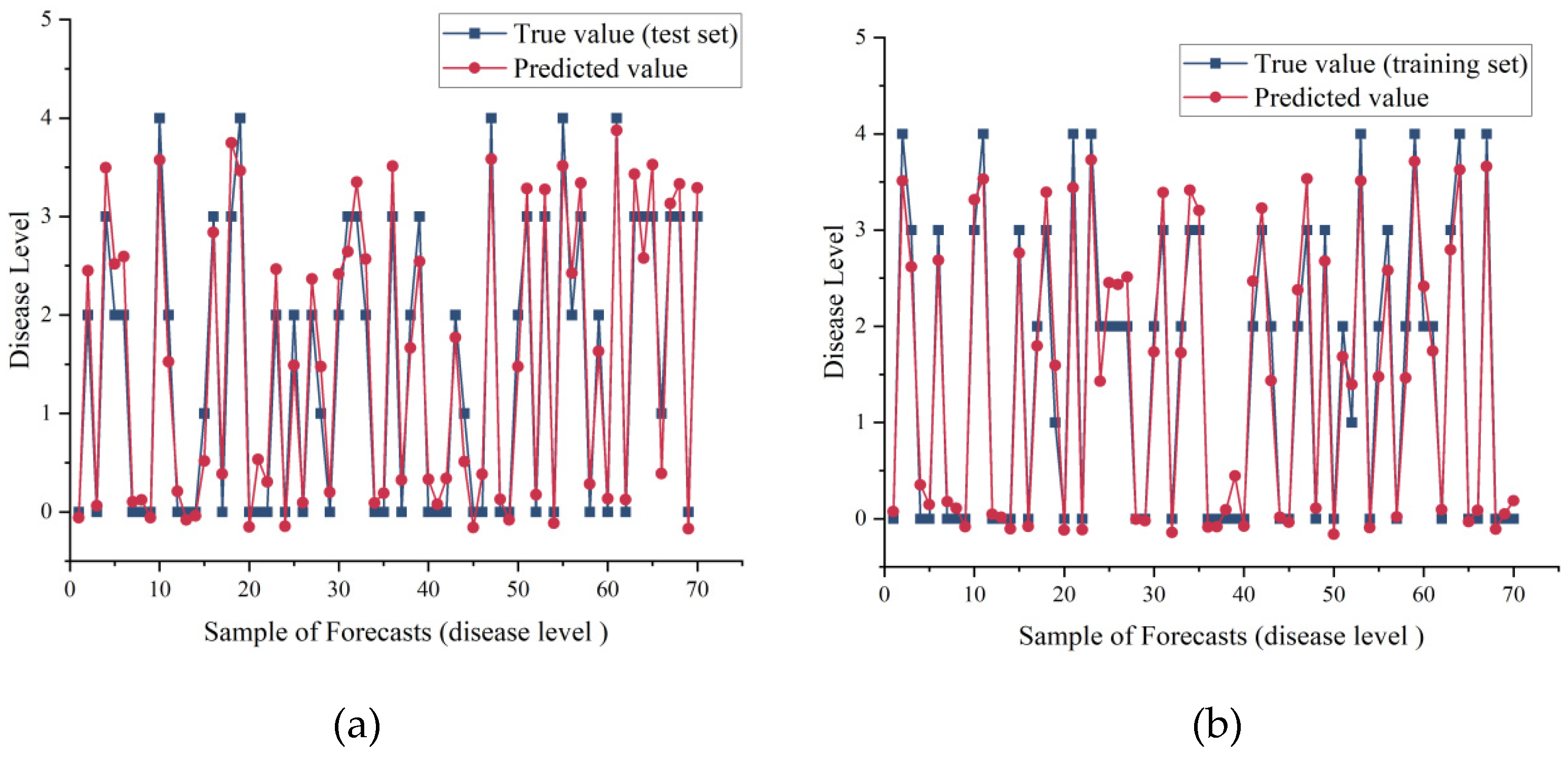
For the disease level, we also obtained better prediction results (
Figure 6). We found that although there were differences in the prediction results of the improved network, the error was extremely small after we rounded the prediction results of the disease level, and by using the disease level 0 and 1 as well as the survey of onset times over the years, we could predict the disease level under future weather forecasts and subsequently infer the onset times.
3.3. Comparison of Prediction Models
Since the improved model combines CNN, LSTM and SE attention mechanism, we compared the performance of CNN, LSTM and the improved model under the same training parameters and environment. From
Table 3, the performance of either the single CNN model or the LSTM model, or the CNN-LSTM model combining the two, was worse than the improved model. Focusing on the test data, the
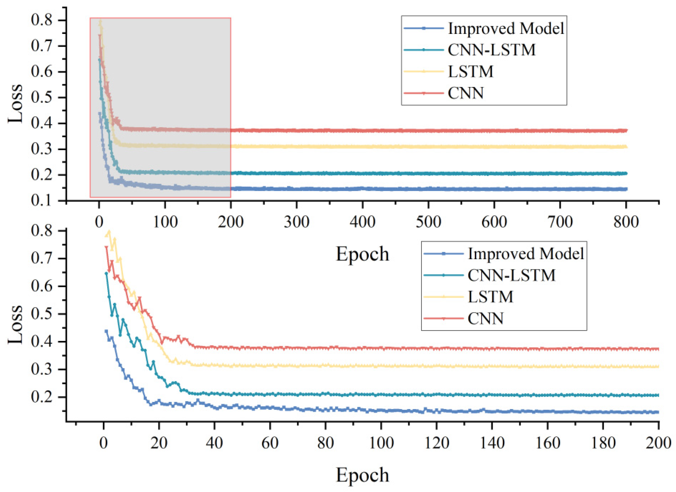
of the improved network was 0.121, 0.155, and 0.013 higher than that of the LSTM, CNN, and CNN-LSTM, in that order, and the RMSE decreased by 0.204, 0.253, and 0.019, in that order. In the loss curves of the training process, we observed that the loss of the improved model was consistently underneath that of the remaining three models. In particular, for the first 200 Epochs (bottom half of
Figure 7), the improved model converged rapidly at the beginning of training (first 20 Epochs), and the loss still fluctuated up to 50 Epochs, and then decays and stabilizes at about 200 Epochs. This showed that the model achieves our expected results.
In addition we included the classic BP neural network and the generalized regression neural network GRNN in the field of deep learning in the comparison. In order to ensure the rationality of the experiment, we also set the same training conditions (hardware environment and model hyperparameters). We found through
Table 3 that the
index of GRNN model on the training set was as high as 0.994, which has exceeded the improved model, but for the test set GRNN
was only 0.811, which is anomalous performance through the actual test results, so we believed that the trained GRNN was an overfitting state. For the BP neural network, the
of the improved model was 0.496 higher than it, and the MAE, MBE, and RMSE were decreased by 0.085, 0.007, and 0.155, respectively. Collectively, the improved model has the best performance in predicting peanut leaf spot disease.
3.2. Practical validation of the model
Authors should discuss the results and how they can be interpreted from the perspective of previous studies and of the working hypotheses. The findings and their implications should be discussed in the broadest context possible. Future research directions may also be highlighted.
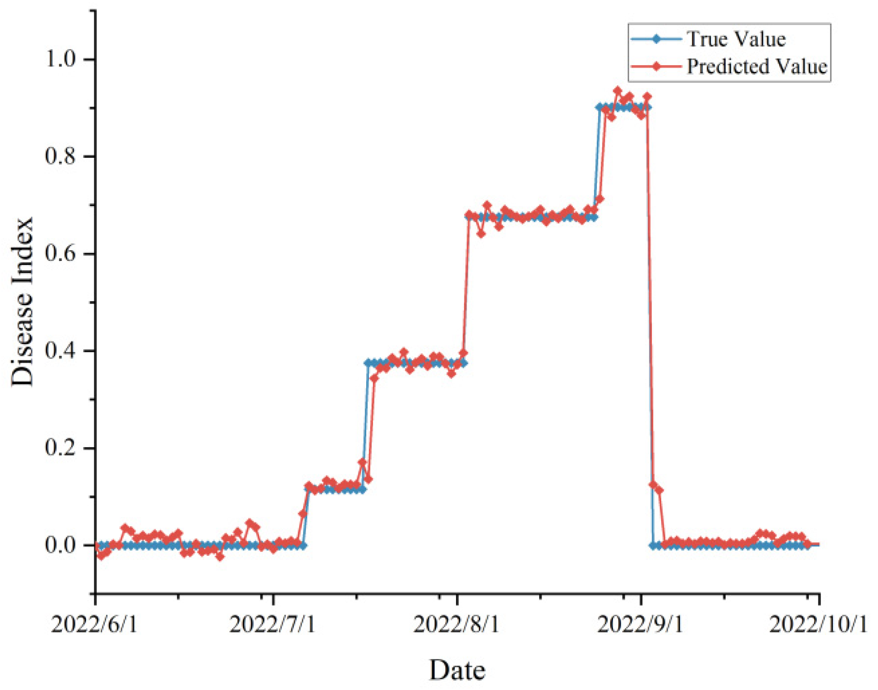
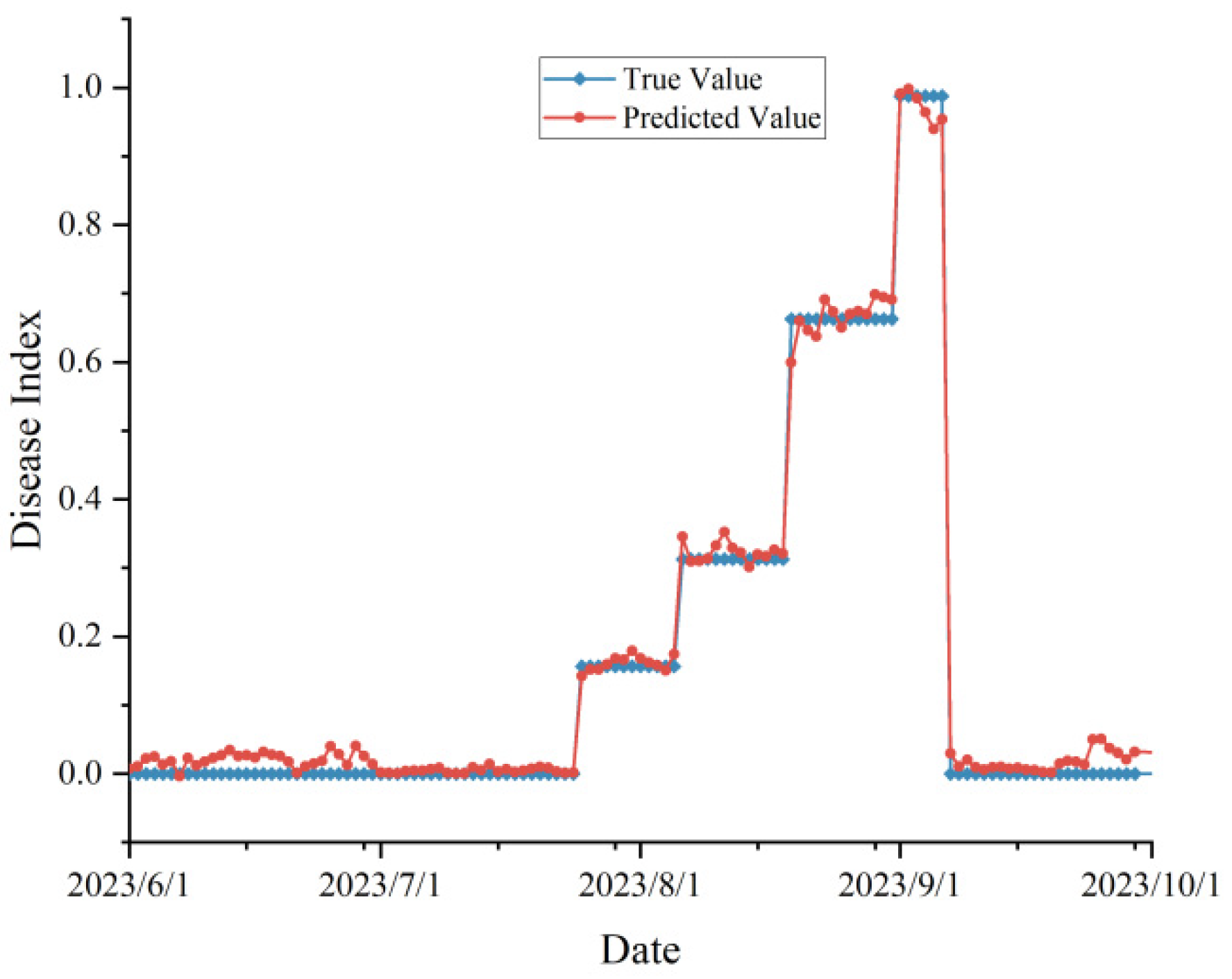
In order to practically test the robustness of our proposed model in real agricultural production scenarios, we investigated the peanut leaf spot disease occurrence in 2022 and 2023, and also obtained the meteorological data from June to September (peanut planting season) of these two years through the Open-Meteo interface. We used the day-by-day meteorological data and time series as inputs to the improved model, or to obtain the prediction results of the disease index, and compared them with the actual surveyed disease occurrence, and the validation results were shown in
Figure 8 and
Figure 9.
In the validation experiment, we predicted disease occurrence based on time scales (without randomly upsetting the data). Since the disease surveys in 2022 and 2023 were not conducted on a day-by-day basis, they were adjusted to a stage-specific disease index when the data were organized. From the figure, the predicted and actual values are highly consistent with each other, and there was no prediction abnormality, which proved that the proposed model was not overfitting and achieves our expected effect. According to the evaluation indexes, the , MAE, MBE, and RMSE of the data in 2022 were 0.932, 0.043, -0.018, and 0.067, respectively, and the indexes in 2023 were 0.938, 0.045, 0.012, and 0.052, respectively, which was a satisfactory result.
4. Conclusions
For consecutive years of meteorological data and peanut leaf spot disease records, we investigated the use of CNN, SE Block and LSTM to build a prediction model for peanut leaf spot disease. Among many deep learning models, by analyzing the relevance and expected goals of each module, we obtained an enhanced LSTM peanut leaf spot disease prediction model to predict its disease index and disease grade with R^2 and RMSE of 0.951 and 0.063, respectively. Through hyper-parameter optimization, it was established that when the learning rate was 0.001, the optimizer was Adma, and the number of cycles was 800, the improved network .odel achieved the best performance on the test set. The experimental results demonstrated that the use of meteorological data and the enhanced LSTM model had certain application value for timely and accurate prediction of peanut leaf spot disease.
Author Contributions
Conceptualization, D.S., Y.C. and M.L.; Methodology, M.L., Z.G. and D.S.; Software, D.S.; Validation, X.C. and Z.G; Formal analysis, Z.G.; Investigation, D.S.,Z.G. and X.C; Resources, M.L. and Z.G.; Data curation, Z.G.,X.C. and D.S.; Writing—original draft preparation, Z.Z. and D.S.; Writing—review and editing, D.S.; Manuscript revising, Z.G. and M.L.; Study design, Z.Z., X.C. and D.S.; Supervision, M.L., Y.C. and D.S.; Project administration, M.L. and Y.C.; Funding acquisition, Y.C. and M.L. All authors have read and agreed to the published version of the manuscript.
Funding
This research was funded by National Natural Science Foundation of China (31972967), National Key Technology Research and Development Program of China (2022YFE0199500), the EU FP7 Framework Program (PIRSES-GA-2013-612659), and Shandong Academy of Agricultural Sciences innovation project (CXGC2023G35).
Data Availability Statement
Not applicable.
Conflicts of Interest
The authors declare no conflict of interest.
References
- Guan, Q.; Song, K.; Feng, S.; Yu, F.; Xu, T. Detection of Peanut Leaf Spot Disease Based on Leaf-, Plant-, and Field-Scale Hyperspectral Reflectance. Remote Sensing. 2022, 14, 4988. [Google Scholar] [CrossRef]
- Partel, V.; Charan Kakarla, S.; Ampatzidis, Y. Development and evaluation of a low-cost and smart technology for precision weed management utilizing artificial intelligence. Computers and Electronics in Agriculture. 2019, 157, 339–350. [Google Scholar] [CrossRef]
- Mueller, D.S.; Bradley, C.A.; Grau, C.R.; Gaska, J.M.; Kurle, J.E.; Pedersen, W.L. Application of thiophanate-methyl at different host growth stages for management of sclerotinia stem rot in soybean. Crop Protection. 2004, 23, 983–988. [Google Scholar] [CrossRef]
- Buja, I.; Sabella, E.; Monteduro, A.G.; Chiriacò, M.S.; De Bellis, L.; Luvisi, A.; Maruccio, G. Advances in plant disease detection and monitoring: From traditional assays to in-field diagnostics. Sensors 2021, 21, 2129. [Google Scholar] [CrossRef] [PubMed]
- Martinelli, F.; Scalenghe, R.; Davino, S.; Panno, S.; Scuderi, G.; Ruisi, P.; Villa, P.; Stroppiana, D.; Boschetti, M.; Goulart, R.L.; et al. Advanced methods of plant disease detection. A review. Agronomy for Sustainable Development 2015, 35, 1–25. [Google Scholar] [CrossRef]
- Islam, M.M.; Adil MA, A.; Talukder, M.A.; Ahamed MK, U.; Uddin, M.A.; Hasan, M.K.; Debnath, S.K. DeepCrop: Deep learning-based crop disease prediction with web application. Journal of Agriculture and Food Research 2023, 14, 100764. [Google Scholar] [CrossRef]
- Fenu, G.; Malloci, F.M. Forecasting plant and crop disease: an explorative study on current algorithms. Big Data and Cognitive Computing 2021, 5, 2. [Google Scholar] [CrossRef]
- Delnevo, G.; Girau, R.; Ceccarini, C.; Prandi, C. A deep learning and social iot approach for plants disease prediction toward a sustainable agriculture. IEEE Internet of Things Journal 2021, 9, 7243–7250. [Google Scholar] [CrossRef]
- Bhatia, A.; Chug, A.; Prakash Singh, A. Application of extreme learning machine in plant disease prediction for highly imbalanced dataset. Journal of Statistics and Management Systems 2020, 23, 1059–1068. [Google Scholar] [CrossRef]
- Azadbakht, M.; Ashourloo, D.; Aghighi, H.; Radiom, S.; Alimohammadi, A. Wheat leaf rust detection at canopy scale under different LAI levels using machine learning techniques. Computers and Electronics in Agriculture 2019, 156, 119–128. [Google Scholar] [CrossRef]
- Yuan, J.; Wen, T.; Zhang, H.; Zhao, M.; Penton, C.R.; Thomashow, L.S.; Shen, Q. Predicting disease occurrence with high accuracy based on soil macroecological patterns of Fusarium wilt. The ISME Journal 2020, 14, 2936–2950. [Google Scholar] [CrossRef]
- Janiesch, C.; Zschech, P.; Heinrich, K. Machine learning and deep learning. Electronic Markets 2021, 31, 685–695. [Google Scholar] [CrossRef]
- Dargan, S.; Kumar, M.; Ayyagari, M.R.; Kumar, G. A survey of deep learning and its applications: a new paradigm to machine learning. Archives of Computational Methods in Engineering 2020, 27, 1071–1092. [Google Scholar] [CrossRef]
- Sherstinsky, A. Fundamentals of recurrent neural network (RNN) and long short-term memory (LSTM) network. Physica D: Nonlinear Phenomena 2020, 404, 132306. [Google Scholar] [CrossRef]
- Zargar, S. Introduction to sequence learning models: RNN, LSTM, GRU. Department of Mechanical and Aerospace Engineering, North Carolina State University, Raleigh, North Carolina, 2021, 27606.
- Bhattacharyya, D.; Joshua ES, N.; Rao, N.T.; Kim, T.H. Hybrid CNN-SVM Classifier Approaches to Process Semi-Structured Data in Sugarcane Yield Forecasting Production. Agronomy 2023, 13, 1169. [Google Scholar] [CrossRef]
- Cao, J.; Wang, J. Stock price forecasting model based on modified convolution neural network and financial time series analysis. International Journal of Communication Systems 2019, 32, e3987. [Google Scholar] [CrossRef]
- Li, M.; Yan, C.; Liu, W. The network loan risk prediction model based on Convolutional neural network and Stacking fusion model. Applied Soft Computing 2021, 113, 107961. [Google Scholar] [CrossRef]
- Juroszek, P.; Racca, P.; Link, S.; Farhumand, J.; Kleinhenz, B. Overview on the review articles published during the past 30 years relating to the potential climate change effects on plant pathogens and crop disease risks. Plant pathology 2020, 69, 179–193. [Google Scholar] [CrossRef]
- Prank, M.; Kenaley, S.C.; Bergstrom, G.C.; Acevedo, M.; Mahowald, N.M. Climate change impacts the spread potential of wheat stem rust, a significant crop disease. Environmental Research Letters 2019, 14, 124053. [Google Scholar] [CrossRef]
- Burdon, J.J.; Zhan, J. Climate change and disease in plant communities. PLoS biology 2020, 18, e3000949. [Google Scholar] [CrossRef]
- Xiao, Q.; Li, W.; Kai, Y.; Chen, P.; Zhang, J.; Wang, B. Occurrence prediction of pests and diseases in cotton on the basis of weather factors by long short term memory network. BMC bioinformatics 2019, 20, 1–15. [Google Scholar] [CrossRef]
- Yu, Y.; Si, X.; Hu, C.; Zhang, J. A review of recurrent neural networks: LSTM cells and network architectures. Neural computation 2019, 31, 1235–1270. [Google Scholar] [CrossRef]
- Sherstinsky, A. Fundamentals of recurrent neural network (RNN) and long short-term memory (LSTM) network. Physica D: Nonlinear Phenomena 2020, 404, 132306. [Google Scholar] [CrossRef]
- Hu, J.; Shen, L.; Sun, G. (2018). Squeeze-and-excitation networks. In Proceedings of the IEEE conference on computer vision and pattern recognition (pp. 7132-7141).
- Larcher, C.H.; Barbosa, H.J. (2021). Evaluating Models with Dynamic Sampling Holdout. In Applications of Evolutionary Computation: 24th International Conference, EvoApplications 2021, Held as Part of EvoStar 2021, Virtual Event, April 7–9, 2021, Proceedings 24 (pp. 729-744).
- Postalcıoğlu, S. Performance analysis of different optimizers for deep learning-based image recognition. International Journal of Pattern Recognition and Artificial Intelligence 2020, 34, 2051003. [Google Scholar] [CrossRef]
- Kingma, D.P.; Ba, J. Adam: A method for stochastic optimization. arXiv 2014, arXiv:1412.6980. [Google Scholar]
- Dogo, E.M.; Afolabi, O.J.; Nwulu, N.I.; Twala, B.; Aigbavboa, C.O. (2018, December). A comparative analysis of gradient descent-based optimization algorithms on convolutional neural networks. In 2018 international conference on computational techniques, electronics and mechanical systems (CTEMS) (pp. 92-99). IEEE.
|
Disclaimer/Publisher’s Note: The statements, opinions and data contained in all publications are solely those of the individual author(s) and contributor(s) and not of MDPI and/or the editor(s). MDPI and/or the editor(s) disclaim responsibility for any injury to people or property resulting from any ideas, methods, instructions or products referred to in the content. |
© 2023 by the authors. Licensee MDPI, Basel, Switzerland. This article is an open access article distributed under the terms and conditions of the Creative Commons Attribution (CC BY) license (http://creativecommons.org/licenses/by/4.0/).
