Preprint
Article

Statistical Inference for Interval-Valued Spatial Error Models

Altmetrics

Downloads

86

Views

10

Comments

0

This version is not peer-reviewed

Submitted:

22 December 2023

Posted:

22 December 2023

You are already at the latest version

Alerts
Abstract
In this paper, we shall introduce the interval-valued spatial error model. Based on the idea of least square method of single-valued case, we give the parameter estimator for interval-valued spatial error model. The theoretical properties of the proposed estimator are proved. Finally, we give the numerical analysis and a real example.
Keywords: 
Subject: Computer Science and Mathematics  -   Probability and Statistics

1. Introduction

It is well known that classical linear regression model and time series models are most widely used in statistical inference, including medical treatment, education, finance, science, technology and many other fields. Most of the cases, these models are used for single-valued random variables. In the real world, there are plenty of random phenomenas cannot be characterized by single-valued random variables. Taking the price of a stock on a given day for example, it is clearly unreasonable to use a single-valued data to decribe the stock price. If only single-valued data such as stock closing price or opening price are used, the fluctuation information in the process of stock trading is ignored and the resulting analysis results provided to decision-makers are also one-sided. Moreover, people will pay more attention to the data in a certain range, such as the temperature for a given day, instead of knowing the temperature at a certain time of one day, people care more about the maximum and minimum temperature of one day. In economic forecasting, economists mostly give a prediction range of economic growth rate. In the process of medical impact diagnosis, the impact result is usually a two-dimensional plan, and it is not a single value. Therefor, the interval-valued data are more appropriate and valuable in these cases because they provide more information. Thus it is necessary to consider the interval-valued statistical models and statictical inference problems.
Interval-valued random variables are special set-valued random variables. In mid twentith century, Aumann and Debreu first used set-valued mapping when studying economic phenomena. Aumann [1] gave the integral of set-valued random variables in 1965. Hiai and Umegaki [6] gave the concept of conditional expectation of set-valued random variables in 1978. Lyashenko [11,12] discussed the properties of set-valued random variables in Euclidean space, introduced the definition of set-valued Gaussian random variables, and gave the definition of variance for set-valued random variables. Vitale [16] studied the properties of D p distance. In 2005, Xuhua Yang and Shoumei Li [17] gave the definitions of variance and covariance for set-valued random variables under the D p distance, and obtained excellent properties. In 2008, Blanco et. al. defined the variance and studied the properties of interval valued random variables under a new distance in [2]. Hess [5], Papageorgiou [14,15], Shoumei Li et. al. [7,8,9] explored the convergence theory of set-valued random variables under different conditions. Molchanov in [13], Shoumei Li et. al. in [10] systematically summarized the theory of set-valued random variables. The above research promoted the development of set-valued random variable theory.
For interval-valued statistical models, Billard and Diday [3] established a linear regression model by using the midpoint of interval-valued random variables in 2000. In 2002, Billard and Diday [4] established linear regression models by using the two endpoints of interval-valued random variables respectively. In 2008, Lima Neto and de Carvalho [19] established linear regression models by using the center and radius of interval-valued random variables. In 2010, Lima Neto and de Carvalho [20] imposed non-negative constraints on the regression coefficients of radius on the basis of [19]. Wang [22] in 2012 proposed the complete information method to deal with the interval-valued linear regression model. Souza [23] introduced the parametrization method to linear regression model in 2017. In 2015, Wang Xun et. al. in [24] used set-valued theory to study linear regression problems, and gave the least square estimaor and the related properties. All the above research works are about the linear regression models of interval-valued random variables. The research on interval-valued spatial regression models and spatial error models are still blank.
As for the single-valued spatial error model, Anselin gave the maximum likelihood estimation method in [26] in 1988. Prucha proposed the generalized moment estimation method in [27] in 1999. In 2020, Yildirim [25] systematically summarized the methods of parameter estimation of spatial error model and proposed a new parameter estimation method based on likelihood equation. Many scholars have studied the classical linear regression and time series models of interval-valued random variables and achieved wonderful research results. We are considering the interval-valued spatial error models.
This paper attempts to extend the classical spatial error model to interval-valued case. The orginazation of this paper is as follows: in Section 2, we mainly introduce the notations and basic concepts of interval-valued random theory. In Section 3, we mainly discuss the interval-valued spatial error model, give the least square estimator of parameter obtain a series of digital characteristics and consistency of parameter estimation; In Section 4, the effectiveness of the method is illustrated by numerical simulation; In Section 5, gives an application of the model by studying the relationship between temperature and latitude in major cities of China.

2. Preliminaries on interval-valued random variables

2.1 d p distance and D p distance

Throughout this paper, we assume that ( Ω , A , μ ) is a complete probability space. R d is a d-dimensional Euclidean space, · and · , · are the norm and inner product in R d respectively, and the family of compact convex subsets in R d is K k c ( R d ) . When d = 1 , R 1 is abbreviated as R , then K k c ( R ) is a family of nonempty bounded closed intervals in R , that is
K k c ( R ) = { A = [ a ̲ , a ¯ ] : < a ̲ a ¯ < , a ̲ , a ¯ R } ,
Where, a ̲ and a ¯ are the left and right endpoints of interval A respectively. In addition, interval A is also denoted as center radius form A = ( c A ; r A ) , where c A = ( a ¯ + a ̲ ) / 2 and r A = ( a ¯ a ̲ ) / 2 are the center and radius of interval A respectively. For any set A, B, the addition and multiplication operations are defined as:
A + B = { a + b : a A , b B } ,
k A = { k a : a A } , k R .
Interval is a special case of set, for A = [ a ̲ , a ¯ ] = ( c 1 ; r 1 ) , B = [ b ̲ , b ¯ ] = ( c 2 ; r 2 ) , the addition and multiplication operations are defined as:
A + B = [ a ̲ + b ̲ , a ¯ + b ¯ ] = ( c 1 + c 2 ; r 1 + r 2 ) , k A = [ k a ̲ , k a ¯ ] , k 0 [ k a ¯ , k a ̲ ] , k < 0 = ( k c 1 ; | k | r 1 ) .
Note that if set A does not degenerate to a point, A A = A + ( A ) { 0 } . Then K k c ( R d ) is not a linear space with respect to addition and multiplication.
For any set A, B in K k c ( R d ) , the subtraction operation is defined as: A B = { a b : a A , b B } . As a special case of set value, for interval A = [ a ̲ , a ¯ ] = ( c 1 ; r 1 ) , B = [ b ̲ , b ¯ ] = ( c 2 ; r 2 ) , the definition of subtraction operation is derived as follows:
A B = [ a ̲ b ̲ , a ¯ b ¯ ] = ( c 1 c 2 ; r 1 + r 2 ) .
The support function of set A K k c ( R d ) is defined as
s ( x , A ) = sup a A x , a , x R d .
The d p distance is defined as follows: for any 1 p < , the d p distance between set A and B is
d p ( A , B ) = S d 1 | s ( x , A ) s ( x , B ) | p d μ ( x ) 1 p , 1 p < ,
where, S d 1 is the unit sphere of R d , μ is a measure on S d 1 , in particular, take μ ( 1 ) = μ ( 1 ) = 1 on S 0 . Further, from Yang and Li [17], ( K k c ( R d ) , d p ) is a complete separable space. Specially, for interval A = [ a ̲ , a ¯ ] = ( c A ; r A ) and B = [ b ̲ , b ¯ ] = ( c B ; r B ) , the d p distance is
d p ( A , B ) = | b ̲ a ̲ | p + | b ¯ a ¯ | p 1 p = [ ( ( c B c A ) ( r B r A ) ) p + ( ( c B c A ) + ( r B r A ) ) p ] 1 p .
In particular, if p = 2 ,
d 2 ( A , B ) = [ ( b ̲ a ̲ ) 2 + ( b ¯ a ¯ ) 2 ] 1 2 = ( ( c B c A ) ( r B r A ) ) 2 + ( ( c B c A ) + ( r B r A ) ) 2 1 2 = [ 2 ( c B c A ) 2 + ( r B r A ) 2 ] 1 2 .
Call set-valued mapping F : Ω K k c ( R d ) be a set-valued random variable, if for any closed sets C K k c ( R d ) ,
F 1 ( C ) = { ω Ω : F ( ω ) C } A .
Let U [ Ω , K k c ( R d ) ] denote the family of set-valued random variables in K k c ( R d ) . The expression of D p distance between set-valued random variables F 1 and F 2 is
D p ( F 1 , F 2 ) = [ E d p p ( F 1 , F 2 ) ] 1 p .
Similarly, for interval-valued random variables, the D p distance between interval value random variables F 1 = [ f ̲ 1 , f ¯ 1 ] = ( c F 1 ; r F 1 ) and F 2 = [ f ̲ 2 , f ¯ 2 ] = ( c F 2 ; r F 2 ) is
D p ( F 1 , F 2 ) = E ( f ̲ 2 f ̲ 1 ) p + E ( f ¯ 2 f ¯ 1 ) p 1 p = E ( ( c F 2 c F 1 ) ( r F 2 r F 1 ) ) p + E ( ( c F 2 c F 1 ) + ( r F 2 r F 1 ) ) p 1 p .
Further, from Yang and Li [17], ( K k c ( R d ) , D p ) is a complete separable distance space. In particular, if p = 2 ,
D 2 ( F 1 , F 2 ) = E ( f ̲ 2 f ̲ 1 ) 2 + E ( f ¯ 2 f ¯ 1 ) 2 1 2 = E ( ( c F 2 c F 1 ) ( r F 2 r F 1 ) ) 2 + E ( ( c F 2 c F 1 ) + ( r F 2 r F 1 ) ) 2 1 2 .

2.2 Moment of set-valued random variables

The expectation of set-valued random variable F U [ Ω , K k c ( R d ) ] is given by Aumann in [1],
E [ F ] = Ω F d ¯ = Ω f d ¯ : f S F ,
where S F is the integrable selection set of F, that is,
S F = { f L p [ Ω , R d ] : f ( ω ) F ( ω ) a . e . ( μ ) } .
Yang and Li in [17] introduced the variance and covariance of set-valued random variables based on D p distance. For set-valued random variable F U [ Ω , K k c ( R d ) ] , the variance is defined as follows:
Var ( F ) = D 2 2 ( F , E [ F ] ) = E d 2 2 ( F , E [ F ] ) = E S d 1 s ( x , F ) s ( x , E [ F ] ) 2 d μ ( x ) .
For two set-valued random variables F 1 , F 2 U [ Ω , K k c ( R d ) ] , the covariance is defined as follows
Cov ( F 1 , F 2 ) = E S d 1 ( s ( x , F 1 ) s ( x , E [ F 1 ] ) ) ( s ( x , F 2 ) s ( x , E [ F 2 ] ) ) d μ ( x ) .
If F = ( c F ; r F ) is an interval-valued random variable, then
Var ( F ) = E [ f ̲ E [ f ̲ ] ] 2 + E [ f ¯ E [ f ¯ ] ] 2 = E ( c F E [ c F ] ) ( r F E [ r F ] ) 2 + E ( c F E [ c F ] ) + ( r F E [ r F ] ) 2 .
The covariance of interval-valued random variables F 1 , F 2 U [ Ω , K k c ( R ) ] is
Cov ( F 1 , F 2 ) = E ( f ̲ 1 E [ f ̲ 1 ] ) ( f ̲ 2 E [ f ̲ 2 ] ) ] + E [ ( f ¯ 1 E [ f ¯ 1 ] ) ( f ¯ 2 E [ f ¯ 2 ] ) = E ( c F 1 E [ c F 1 ] ( r F 1 E [ r F 1 ] ) ) ( c F 2 E [ c F 2 ] ( r F 2 E [ r F 2 ] ) ) + E ( c F 1 E [ c F 1 ] + ( r F 1 E [ r F 1 ] ) ) ( c F 2 E [ c F 2 ] + ( r F 2 E [ r F 2 ] ) ) .
Through calculation, we can easily have
Var ( F ) = 2 E [ c F E [ c F ] ] 2 + 2 E [ r F E [ r F ] ] 2 = 2 Var ( c F ) + 2 Var ( r F ) ,
Cov ( F 1 , F 2 ) = 2 E ( c F 1 E [ c F 1 ] ) ( c F 2 E [ c F 2 ] ) + 2 E ( r F 1 E [ r F 1 ] ) ( r F 2 E [ r F 2 ] ) = 2 Cov ( c F 1 , c F 2 ) + 2 Cov ( r F 1 , r F 2 ) .
The variance and covariance of interval-valued random variables will be used in Section 3. For more information about the variance and covariance of set-valued random variables, readers can refer to [17].

3. Interval-valued spatial error model

Y = X β + u , u = λ w u + ε , | λ | < 1 .
Consider the classical spatial error model with the following form, where X is the explanatory variable, Y is the explained variable, β is the unknown parameter, error term u, and ε are single point values, and W is a known n × n space weight matrix, λ is a spatial autoregressive coefficient parameter,
the error item ε N ( 0 , σ 2 I n ) , I n is an identity matrix. By transforming, model (3.1) becomes,
( I n λ W ) Y = I n λ W X β + ε ,
denoted by
Y λ = I n λ W Y , X λ = I n λ W X ,
Model (3.2) can be expressed as
Y λ = X λ β + ε ,
E ( Y λ ) = X λ β .
Now we extend the above classical single-valued model to interval-valued case.
Definition 3.1 If Y λ = ( Y λ 1 , Y λ 2 , , Y λ n ) T is the n-dimensional vector of interval-valued observations, X λ = ( x λ i j ) n × p is the n × p single point valued design matrix, β = ( β 1 , β 2 , , β p ) is a p-dimensional interval-valued parameter vector, then model (3.3), is called interval-valued space error model.
Next, we give the algorithm for multiplication of the matrix and interval values.
Definition 3.2 Let A i = [ a i ̲ , a i ¯ ] = ( c i ; r i ) , i = 1 , , p be the interval in K k c ( R ) , the interval value vector A = ( A 1 , A 2 , , A p ) T is multiplied by any n × p dimensional matrix ( m i j ) n × p , i = 1 , 2 , , n ; j = 1 , 2 , , p , the algorithm is defined as follows:
( m i j ) n × p A = m 11 A 1 + + m 1 p A p m n 1 A 1 + + m n p A p = m 11 ( c 1 ; r 1 ) + + m 1 p ( c p ; r p ) m n 1 ( c 1 ; r 1 ) + + m n p ( c p ; r p ) = m 11 [ a 1 ̲ , a 1 ¯ ] + + m 1 p [ a p ̲ , a p ¯ ] m n 1 [ a 1 ̲ , a 1 ¯ ] + + m n p [ a p ̲ , a p ¯ ] .
For the general single-valued linear model, the idea of the least squares estimation method is to minimize the sum of the squares of the residuals. We shall use the same mathematical idea here. For interval-valued spatial error model, the least square estimation of interval-valued unknown parameter β is to minimize d 2 2 ( Y λ , X λ β ) under the definition of d 2 distance
d 2 2 ( Y λ , x λ β ) = i = 1 n d 2 2 Y λ i , x λ i 1 β 1 + x λ i 2 β 2 + + x λ i p β p = i = 1 n c Y λ i x λ i 1 c β 1 x λ i p c β p r Y λ i x λ i 1 r β 1 x λ i p r β p 2 + i = 1 n c Y λ i x λ i 1 c β 1 x λ i p c β p + r Y λ i x λ i 1 r β 1 x λ i p r β p 2 = 2 i = 1 n c Y λ i x λ i 1 c β 1 x λ i p c β p 2 + r Y λ i x λ i 1 r β 1 x λ i p r β p 2 ,
where c m and r m represent the center and radius of interval value m respectively. The above formula is the quadratic function of c β j and r β j , and d 2 2 ( Y λ , X λ β ) 0 , so there is a minimum value.
Next, calculate the partial derivatives of c β j and r β j respectively
d 2 2 ( Y λ , X λ β ) c β j = 0 d 2 2 ( Y λ , X λ β ) r β j = 0 , j = 1 , 2 , , p .
that is,
i = 1 n c Y λ i x λ i 1 c β 1 x λ i p c β p x λ i j = 0 i = 1 n r Y λ i | x λ i 1 | r β 1 | x λ i p | r β p | x λ i j | = 0 .
The regular equation is:
X λ T c Y λ = X λ T X λ c β | X λ | T r Y λ = | X λ | T | X λ | r β ,
where | X λ | = x i j n × p . The parameter estimation of the interval-valued spatial error model can be obtained by solving the regular equation. The following is the result about the rank of X λ .
Lemma 3.3 If r k ( X ) = p , then r k ( X λ ) = p .
Proof Since
r k ( X λ ) = r k ( ( I n λ w ) X ) min ( r k ( I n λ w ) , r k ( X ) ) r k ( X ) = p
and
r k ( ( I n λ w ) X ) r k ( I n λ w ) + r k ( X ) n = p ,
it has
r k ( ( I n λ w ) X ) = r k ( X λ ) = r k ( X ) = p .
The result is proved. □
Based on Lemma 3.3, suppose r k ( | X λ | ) = p , then the estimator of interval-valued spatial error model can be obtained by solving the regular equation, which is shown in the following theorem.
Theorem 3.3 Under the condition of Lemma 3.3, the least squares estimation of interval-valued spatial error model is unique, which is denoted as
β ^ L S ( λ ) = ( ( X λ T X λ ) 1 X λ T c Y λ ; ( | X λ | T | X λ | ) 1 | X λ | T r Y λ ) = ( ( X T ( I n λ W ) T ( I n λ W ) X ) 1 X T ( I n λ W ) T ( I n λ W ) c Y ; ( | X | T | I n λ W | T | I n λ W | | X | ) 1 | X | T | I n λ W | T | I n λ W | r Y ) .
After obtaining the estimation form of unknown parameter β , we then discuss the properties. First, consider the unbiasedness of β ^ L S ( λ ) .
Theorem 3.4 The least squares estimate β ^ L S ( λ ) is an unbiased estimate of β .
Proof By Theorem 3.3,
E ( β ^ L S ( λ ) = ( ( X λ T X λ ) 1 X λ T E [ c Y λ ] ; ( | X λ | T | X λ | ) 1 | X λ | T E [ r Y λ ] ) = E ( ( X T ( I n λ W ) T ( I n λ W ) X ) 1 X T ( I n λ W ) T ( I n λ W ) c Y ; ( | X | T | I n λ W | T | I n λ W | | X | ) 1 | X | T | I n λ W | T | I n λ W | r Y ) = ( ( X T ( I n λ W ) T ( I n λ W ) X ) 1 X T ( I n λ W ) T ( I n λ W ) E ( c Y ) ; ( | X | T | I n λ W | T | I n λ W | | X | ) 1 | X | T | I n λ W | T | I n λ W | E ( r Y ) ) = ( ( X T ( I n λ W ) T ( I n λ W ) X ) 1 X T ( I n λ W ) T ( I n λ W ) X c β ; ( | X | T | I n λ W | T | I n λ W | | X | ) 1 | X | T | I n λ W | T | I n λ W | | X | r β ) = ( c β ; r β ) = β .
The result is proved. □
For the interval-valued spatial error model, when r k ( X λ ) = r k ( X λ ) = p , the covariance of β ^ L S ( λ ) can be obtained, as shown in the following result.
Theorem 3.5 If r k ( X λ ) = r k ( X λ ) = p , E ( Y λ ) = X λ β , C o v ( c Y λ ) = c σ 2 I n , C o v ( r Y λ ) = r σ 2 I n , then the covariance matrix of β ^ L S ( λ ) is
(1) i j ,
C o v β ^ L S ( i ) ( λ ) , β ^ L S ( j ) ( λ ) = 2 c σ 2 ( X λ T X λ ) 1 X λ T ( i ) X λ ( X λ T X λ ) 1 ( j ) + 2 r σ 2 ( | X λ | T | X λ | ) 1 | X λ | T ( i ) | X λ | ( | X λ | T | X λ | ) 1 ( j ) ,
(2) i = j ,
C o v β ^ L S ( i ) ( λ ) , β ^ L S ( j ) ( λ ) = 2 c σ 2 X T ( I n λ W ) T ( I n λ W ) X 1 + 2 r σ 2 | X | T | I n λ W | T | I n λ W | | X | 1 ,
where β ^ L S ( i ) ( λ ) , β ^ L S ( j ) ( λ ) represent the ith and jth element of β ^ L S ( λ ) respectively, and A ( i ) , A ( j ) represent the ith, jth rows of matrix A respectively.
Proof For the ith and jth element of β ^ L S ( λ ) , if i j , it has
C o v β ^ L S ( i ) ( λ ) , β ^ L S ( j ) ( λ ) = C o v { ( ( X λ T X λ ) 1 X λ T ) ( i ) c Y λ ; ( ( | X λ | T | X λ | ) 1 | X λ | T ) ( i ) r Y λ , ( ( X λ T X λ ) 1 X λ T ) ( j ) c Y λ ; ( ( | X λ | T | X λ | ) 1 | X λ | T ) ( j ) r Y λ } = 2 C o v ( ( X λ T X λ ) 1 X λ T ) ( i ) c Y λ , ( ( X λ T X λ ) 1 X λ T ) ( j ) c Y λ + 2 C o v ( ( X λ T X λ ) 1 X λ T ) ( i ) r Y λ , ( ( X λ T X λ ) 1 X λ T ) ( j ) r Y λ = 2 ( X λ T X λ ) 1 X λ T ( i ) C o v ( c Y λ ) ( X λ T X λ ) 1 X λ T ( j ) T + 2 ( | X λ | T | X λ | ) 1 | X λ | T ( i ) C o v ( c Y λ ) | X λ | T | X λ | ) 1 | X λ | T ( j ) T = 2 c σ 2 ( X λ T X λ ) 1 X λ T ( i ) X λ ( X λ T X λ ) 1 ( j ) + 2 r σ 2 ( | X λ | T | X λ | ) 1 | X λ | T ( i ) | X λ | ( | X λ | T | X λ | ) 1 ( j ) .
When i = j , it has
C o v β ^ L S ( i ) ( λ ) , β ^ L S ( i ) ( λ ) = 2 c σ 2 ( X λ T X λ ) 1 + 2 r σ 2 ( | X λ | T | X λ | ) 1 = 2 c σ 2 X T ( I n λ W ) T ( I n λ W ) X 1 + 2 r σ 2 | X | T | I n λ W | T | I n λ W | | X | 1 .
The result is proved. □
Next we discuss the estimation of error ε and error variance. We mainly consider the expectation and covariance of interval-valued error estimation.
Theorem 3.6 The error estimator ε ^ can be obtained from Y λ X λ β ^ L S , and its expectation and variance are as follows:
(1) E ( ε ^ ) = 0 ,
(2) C o v ( ε ^ ) = 2 c σ 2 ( I n P x λ ) + 2 r σ 2 ( I n + P | x λ | ) ,
where P X λ = X λ ( X λ T X λ ) 1 X λ T , P | X λ | = | X λ | ( | X λ | T | X λ | ) 1 | X λ | T .
Proof
(1) Since
ε ^ = Y λ X λ β ^ L S ( λ ) = ( c Y λ ; r Y λ ) X λ ( X λ T X λ ) 1 X λ T c Y λ ; ( | X λ | T | X λ | ) 1 | X λ | T r Y λ = ( c Y λ ; r Y λ ) X λ ( X λ T X λ ) 1 X λ T c Y λ ; | X λ | ( | X λ | T | X λ | ) 1 | X λ | T r Y λ = ( c Y λ ; r Y λ ) ( c Y λ ; r Y λ ) = ( 0 ; 2 r Y λ ) ,
it has
E ( ε ^ ) = E ( Y λ X λ β ^ L S ( λ ) ) = ( X λ c β ; | X λ | r β ) ( X λ ( X λ T X λ ) 1 X λ T X λ c β ; | X λ | ( | X λ | T | X λ | ) 1 | X λ | T | X λ | r β = ( X λ c β ; | X λ | r β ) ( X λ c β ; | X λ | r β ) = ( 0 ; 2 | X λ | r β ) .
(2) On the other hand,
ε ^ = Y λ X λ β ^ L S ( λ ) = ( c Y λ ; r Y λ ) X λ ( X λ T X λ ) 1 X λ T c Y λ ; ( | X λ | T | X λ | ) 1 | X λ | T r Y λ = ( I n X λ ( X λ T X λ ) 1 X λ T ) c Y λ ; ( I n + | X λ | ( | X λ | T | X λ | ) 1 | X λ | T ) r Y λ = ( I n P X λ ) c Y λ ; ( I n + P | X λ | ) r Y λ .
Then the ith element of ε ^ is
( I n P X λ ) ( i ) c Y λ ; ( I n + P | X λ | ) ( i ) r Y λ .
Thus when i j ,
C o v ( ε i ^ , ε j ^ ) = C o v { ( I n P X λ ) ( i ) c Y λ ; ( I n + P | X λ | ) ( i ) r Y λ , ( I n P X λ ) ( j ) c Y λ ; ( I n + P | X λ | ) ( j ) r Y λ } = 2 C o v ( I n P X λ ) ( i ) c Y λ , ( I n P X λ ) ( j ) c Y λ + 2 C o v ( I n + P | X λ | ) ( i ) r Y λ , ( I n + P | X λ | ) ( j ) r Y λ = 2 ( I n P X λ ) ( i ) C o v ( c Y λ ) ( I n P X λ ) ( j ) + 2 ( I n P | X λ | ) ( i ) C o v ( r Y λ ) ( I n + P | X λ | ) ( j ) ,
where A ( i ) , A ( j ) respectively represent the ith and jth rows of matrix A. When i = j ,
C o v ( ε ^ ) = 2 ( I n P X λ ) C o v ( c Y λ ) ( I n P X λ ) + 2 ( I n P | X λ | ) C o v ( r Y λ ) ( I n + P | X λ | ) = 2 c σ 2 ( I n P X λ ) + 2 r σ 2 ( I n + P | X λ | ) .
The result is proved. □
Next, we consider the estimation of c σ 2 = C o v ( c Y λ ) and r σ 2 = C o v ( r Y λ ) . Denote c ^ ε = ( I n P X λ ) c Y λ , r ^ ε = ( I n + P X λ ) r Y λ .
Theorem 3.7  c ^ σ 2 = c ^ ε T c ^ ε n p and r ^ σ 2 = c ^ ε T c ^ ε n + p are unbiased estimators of c σ 2 and r σ 2 respectively.
Proof Since ( I n P X λ ) is an idempotent matrix, it has
c ^ ε T c ^ ε = ( I n P X λ ) c Y λ T ( I n P X λ ) c Y λ = c Y λ T ( I n P X λ ) c Y λ .
So
E [ c ^ ε T c ^ ε ] = E c Y λ T ( I n P X λ ) c Y λ = ( X λ c β ) T ( I n P X λ ) ( X λ c β ) + t r ( I n P X λ ) C o v ( c Y λ ) = c σ 2 t r ( I n P X λ ) = c σ 2 ( n p ) .
Then the estimator of c σ 2 is gived as
c ^ σ 2 = c ^ ε T c ^ ε n p .
So
E ( c ^ σ 2 ) = E ( c ^ ε T c ^ ε n p ) = 1 n p c σ 2 ( n p ) = c σ 2 .
Since ( I n + P | X λ | ) is an idempotent matrix, so
r ^ ε T r ^ ε = ( I n + P | X λ | ) r Y λ T ( I n + P | X λ | ) r Y λ = r Y λ T ( I n + P | X λ | ) r Y λ .
Furthermore
E [ r ^ ε T r ^ ε ] = E r Y λ T ( I n + P | X λ | ) r Y λ = ( | X λ | r β ) T ( I n + P | X λ | ) ( | X λ | r β ) + t r ( I n + P | X λ | ) C o v ( r Y λ ) = r σ 2 t r ( I n + P | X λ | ) = r σ 2 ( n + p ) .
The estimator of r σ 2 is given as
r ^ σ 2 = r ^ ε T r ^ ε n + p .
So
E ( r ^ σ 2 ) = 1 n p r σ 2 ( n p ) = r σ 2 .
The result is proved. □
In the following, we discuss the independence of β ^ L S = ( c ^ β ; r ^ β ) and σ 2 ^ = ( c ^ σ 2 ; r ^ σ 2 ) .
Theorem 3.8  c ^ σ 2 and c ^ β are independent, r ^ σ 2 and r ^ β are independent.
Proof Since
σ 2 ^ = ( c ^ σ 2 ; r ^ σ 2 ) = c Y λ T ( I n P X λ ) c Y λ n p ; r Y λ T ( I n + P | X λ | ) r Y λ n p ,
β ^ L S ( λ ) = ( c ^ β ; r ^ β ) = ( X λ T X λ ) 1 X λ T c Y λ ; ( | X λ | T | X λ | ) 1 | X λ | T r Y λ ,
it can be seen that c ^ σ 2 is the quadratic form of c Y λ , c ^ β is the linear form of c Y λ , and c Y λ N 0 , c σ 2 I n .
According to the independence theorem of quadratic form and linear form of normal variables, it is necessary to prove that they are independent of each other, that is, the product of linear part, variance part and quadratic part of normal variables is 0. Then
( X λ T X λ ) 1 X λ T c σ 2 I n ( I n P X λ ) = c σ 2 I n ( ( X λ T X λ ) 1 X λ T ( X λ T X λ ) 1 X λ T P X λ ) = 0 .
Similarly, r ^ σ 2 is the quadratic form of r Y λ , r ^ β is the linear form of r Y λ , and r Y λ N 0 , r σ 2 I n , then
( | X λ | T | X λ | ) 1 | X λ | T r σ 2 I n ( I n P | X λ | ) = r σ 2 I n ( ( | X λ | T | X λ | ) 1 | X λ | T ( | X λ | T | X λ | ) 1 | X λ | T P | X λ | ) = 0 .
Thus c ^ σ 2 and c ^ β are independent, r ^ σ 2 and r ^ β are independent. □
Theorem 3.9 In the sense of D 2 distance, the sufficient condition for the strong consistentancy of β ^ L S ( λ ) for estimating β is:
lim n ( S n 1 + | S n | 1 ) = 0
where, S n = X λ T X λ , | S n | = | X λ | T | X λ | .
Proof According to Theorem 3.4, β ^ L S ( λ ) is an unbiased estimate of β , namely,
E ( β ^ L S ( λ ) ) = β .
Moreover,
V a r ( β ^ L S ( λ ) ) = 2 c σ 2 ( X T ( I n λ W ) T ( I n λ W ) X ) 1 + 2 r σ 2 ( | X | T | I n λ W | T | I n λ W | | X | ) 1 ) ,
From lim n ( S n 1 + | S n | 1 ) = 0 , it has
lim n V a r ( β ^ L S ( λ ) ) = lim n ( 2 c σ 2 ( X T ( I n λ W ) T ( I n λ W ) X ) 1 + 2 r σ 2 ( | X | T | I n λ W | T | I n λ W | | X | ) 1 ) = lim n ( 2 c σ 2 S n 1 + 2 r σ 2 | S n | 1 ) = 0 .
Thus
lim n V a r ( β ^ L S ( λ ) ) = lim n D 2 2 ( β ^ L S ( λ ) , E ( β ^ L S ( λ ) ) ) = 0 .
Therefore, in the sense of D 2 metric, β ^ L S ( λ ) is a strong consistent estimate of β . □

4. Numerical simulation

In this part, the parameter estimation process of interval-valued spatial error model is further explored by numerical simulation. Based on the d p distance of the interval value, mean square error of the estimator is calculated to measure the goodness of the estimation.
Based on Equation 3.3, the interval-valued spatial error model in matrix form is expanded as follows:
y 1 λ y 2 λ y n λ = 1 x 1 λ 1 x 2 λ 1 x n λ β 1 β 2 + ε 1 ε 2 ε n ,
where
Y λ = y 1 λ , y 2 λ , , y n λ = I n λ W Y X λ = x 1 λ , x 2 λ , , x n λ = I n λ W X .
I n is the unit matrix of dimension n, λ is the spatial autocorrelation coefficient. and W as the spatial weight matrix. Using the first-order adjacency method, assuming that n samples are arranged in one font, the spatial weight matrix can be written as follows:
W = 0 1 0 0 0 1 0 1 0 0 0 1 0 0 0 0 0 0 0 1 0 0 0 1 0 .
The true values of the given interval value parameters are β 1 = [ 1 , 2 ] = ( 1.5 ; 0.5 ) , β 2 = [ 1.5 , 2.5 ] = ( 2 ; 0.5 ) respectively. Then,
y i λ = β 1 + x i λ β 2 + ε i = 1.5 + 2 x i λ + c ε i ; 0.5 + 0.5 x i λ + r ε i ,
where, the error term follows the normal distribution, that is c ε i , r ε i N 0 , 0 . 3 2 .
First, take n = 100 , the explanatory variable X is generated according to the rules of x i = 0.5 + 0.1 i , i = 1 , 2 , , 100 , and a set of values will be obtained in each simulation experiment.
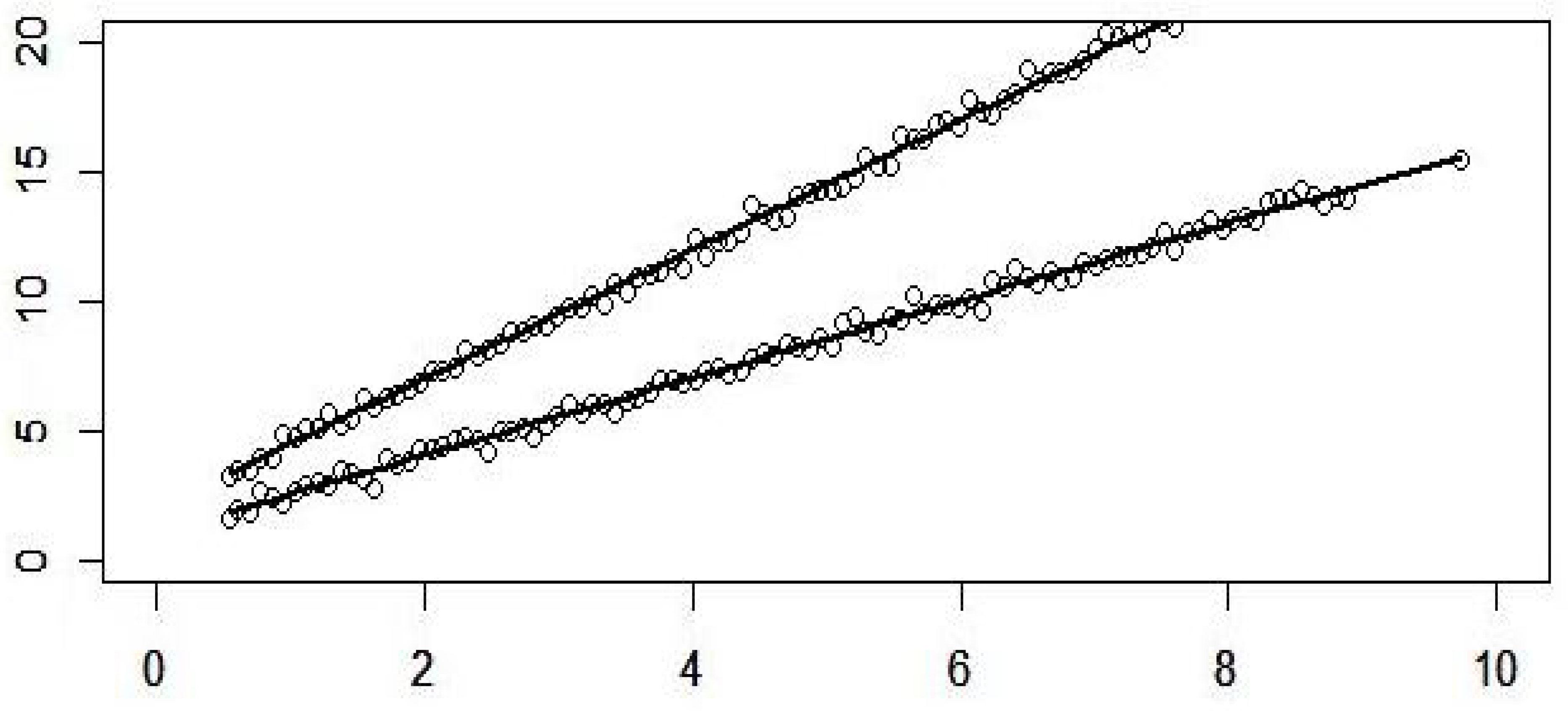
The scatter point in Figure 1 is the y i λ data generated by a simulation experiment, and the two fitting lines are the corresponding interval value spatial error model function:
Y λ = [ 1.0653 , 2.0171 ] + [ 1.4955 , 2.5009 ] X λ .
Repeat the above process for 500 times to obtain the average value of β ^ = ( β ^ 1 , β ^ 2 ) as follows:
β ^ ¯ = ( [ 1.0004 , 2.0019 ] , [ 1.4999 , 2.4999 ] ) .
Next, the mean square error MSE of the parameter estimation obtained by the model is calculated as one of the criteria to measure the goodness of the estimation. The calculation method is based on interval value d p distance:
M S E = 1 n i = 1 n d 2 2 β , β ^ = 1 500 i = 1 500 d 2 2 β , β ^
By calculation, the MSE of samples β ^ 1 , β ^ 2 are 0.0165 and 0.0006 respectively.
Similarly, set n = 200 , n = 300 , repeat the above simulation process for 500 times respectively, and obtain the average value of β ^ = ( β ^ 1 , β ^ 2 ) and the sample mean square error MSE respectively. The specific simulation results are summarized in Table 1 and Table 2.
It can be seen from the simulation results that when n = 100 , the obtained parameter estimation is very close to the real value. With the increase of sample size, the obtained estimation is closer to the real value, and the sample mean square error MSE is smaller and smaller.
5. Empirical analysis

5.1 Data preparation

In this paper, we select the index data of 31 cities from 31 provinces and autonomous regions in China (not considered temporarily due to geographical factors, Hong Kong, Macao and Taiwan) to illustrate the application of interval-valued spatial error model in practice. This section mainly studies factors such as latitude, maximum and minimum temperatures and temperature difference. Due to the vast territory of China, the temperature and latitude of different cities in a region are different. Therefore, the provincial capital cities in various regions are selected as the research object. The temperature data is the minimum and maximum temperature on July 8, 2021. The temperature data comes from Baidu weather forecast, and the latitude data comes from convenient query website( https://jingweidu.bmcx.com/ ), the data indicators are summarized in Table 3.
Before modeling and analysis, spatial autocorrelation test is carried out for the data. First, the spatial autocorrelation test is based on the spatial weight matrix. In this paper, the distance based representation is selected for the selection of the spatial weight matrix. The spatial weight matrix is obtained by the open source software geoda. After obtaining the spatial weight matrix, the matrix is standardized. Of course, there are many representation methods of spatial weight matrix, and distance representation can also be selected, which will not be repeated here. Spatial autocorrelation is based on the explained variable. The explained variable in this paper consists of the interval value of the lowest temperature and the highest temperature. Therefore, in the spatial autocorrelation test, the general linear model can be used to model the upper and lower endpoints of interval values respectively, and the center values of the highest and lowest temperatures can be used for spatial autocorrelation test.
One of the main methods of spatial autocorrelation test is to conduct global or local Moran’s I test. As can be seen from the table below, the global Moran’s I indexes are 0.4193 and 0.3013 respectively, and the tested p values are less than the significant level of 0.05. Therefore, the original hypothesis is rejected and it is considered that the maximum and minimum temperatures of 31 provinces, cities and autonomous regions in China have a certain spatial autocorrelation.
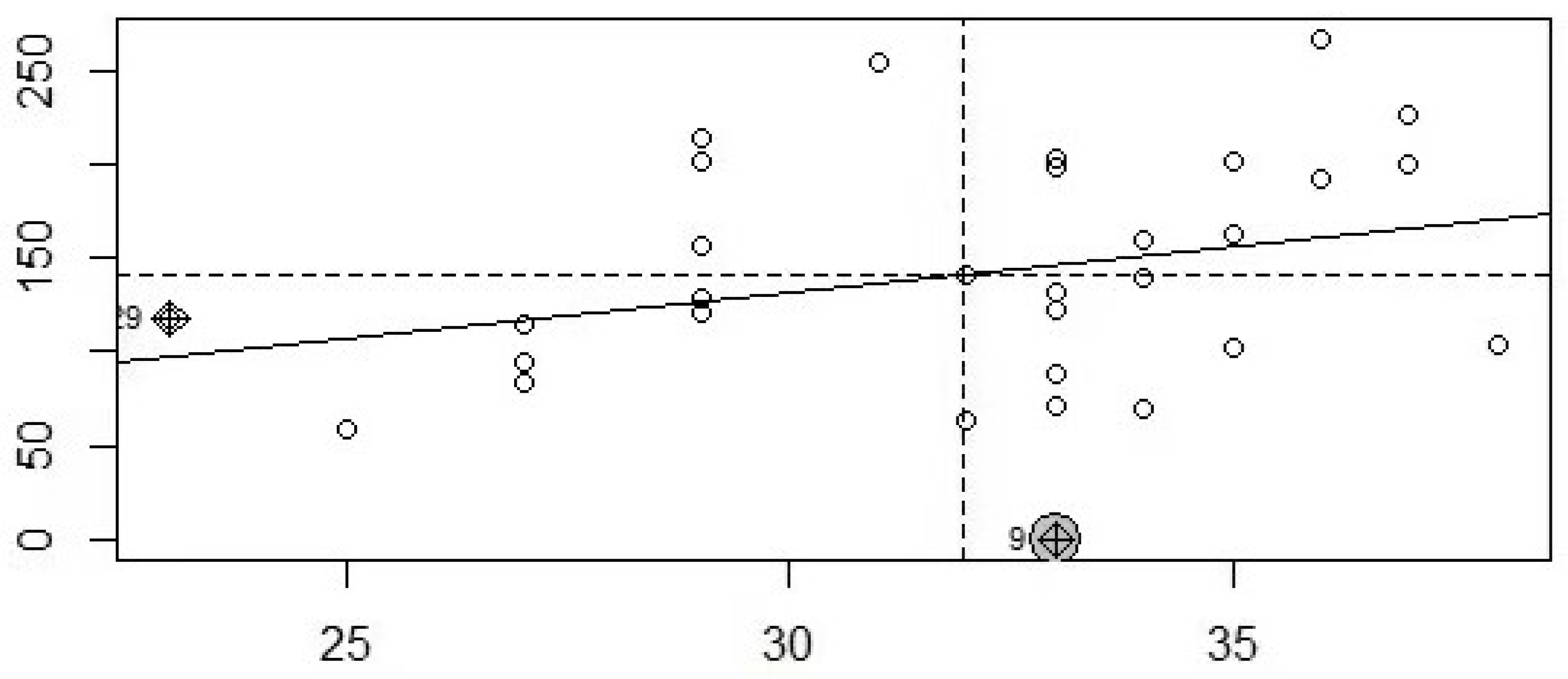
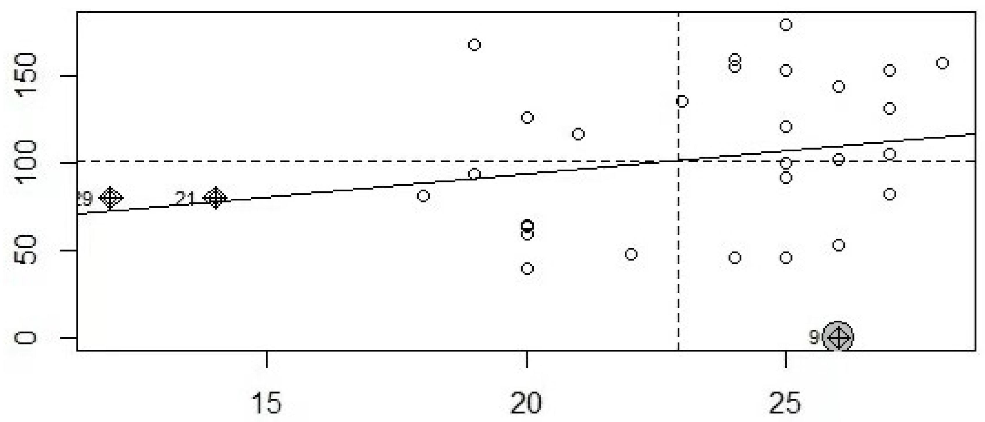
Figure 2 and Figure 3 are the scatter diagrams of global Moran’s I coefficient. It can be seen that the highest and lowest temperatures of 31 regions in China have positive autocorrelation, that is, the trend of high high and low low.

5.2 Parameter estimation of interval-valued spatial error model

After data preparation and spatial autocorrelation test, the interval-value spatial error model is established. Among them, the dependent variable is air temperature, the interval value data is composed of the lowest and highest air temperatures, and the explanatory variable is latitude. The parameter estimation is carried out by the parameter estimation method of interval-value spatial error model in Section 3. It is assumed that the air temperature and latitude conform to the interval-valued linear model, that is:
E ( y i λ ) = β 1 + x i λ β 2
As the method mentioned in Section 4, by the minimum temperature and the maximum temperature we can obtained λ ( λ 1 = 0.1187 , λ 2 = 0.1429 ) respectively. Then take the average value as the λ ( λ = λ 1 + λ 2 2 = 0.1308 ) of the interval-valued spatial error model. GeoDa software is used to obtain the spatial weight matrix of 31 regions. Take the inverse square of the matrix elements, and then standardize to obtain the final spatial weight matrix..
The parameter estimation results are shown in Table 5, which shows that:
β ^ = ( β 1 ^ , β ^ 2 ) = ( [ 24.7501 , 29.5478 ] , [ 0.1681 , 0.0619 ] )
The final interval-valued spatial error model is:
Y λ = [ 24.7501 , 29.5478 ] + [ 0.1681 , 0.0619 ] X λ .
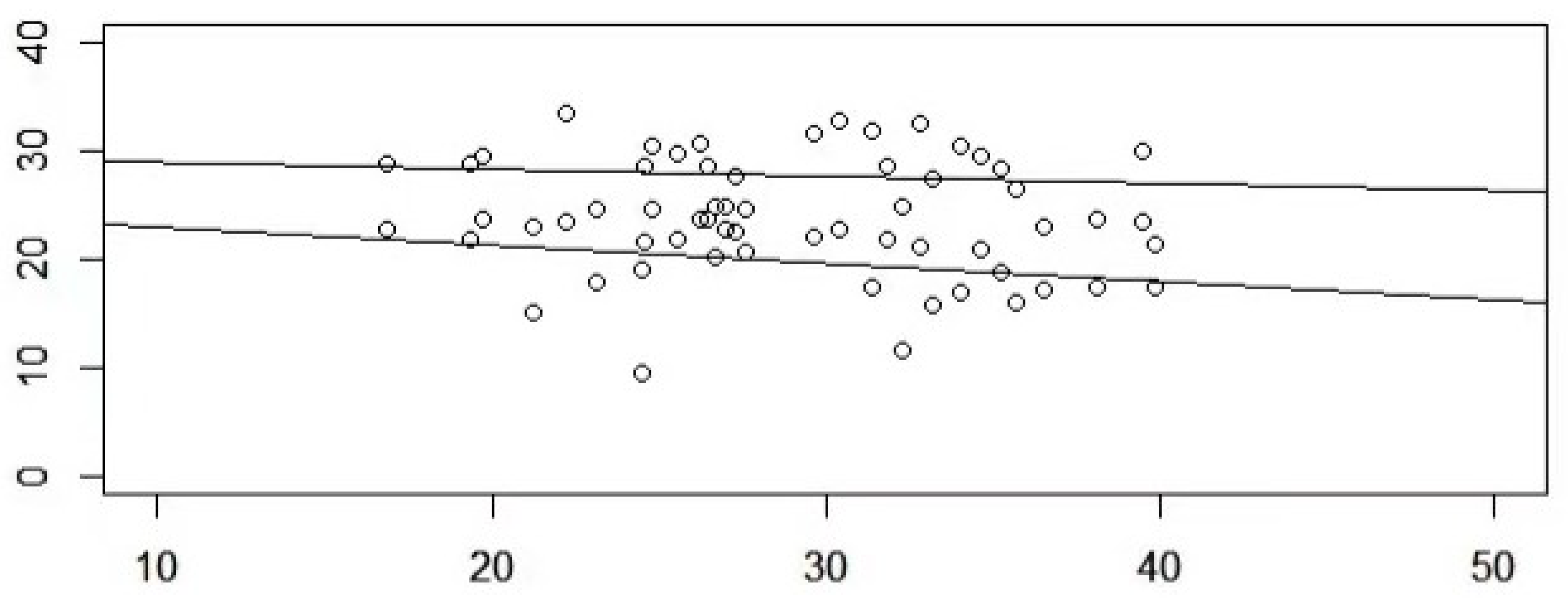
In Figure 4, the abscissa and ordinate are latitude and temperature (maximum temperature and minimum temperature) respectively, it can be seen that the temperature and latitude of the 31 cities in China are negatively correlated. With the increasing of latitude, the temperature has a certain downward trend. At the same time, it can also be seen that the temperature difference (the difference between the maximum temperature and the minimum temperature) tends to expand with the increase of latitude, which is also consistent with the large diurnal temperature difference in northwest and northeast of China. And small temperature difference between day and night in central region of China, southeast and southwest of China.

Acknowledgments

This work is supported by the National Social Science Fund of China No.19BTJ017.

References

  1. Aumann R J. Integrals of set-valued functions[J]. Journal of Mathematical Analysis and Applications, 1965, 12(1): 1-12.
  2. Blanco Fernandez A, Corral N, Gonzalez-Redriguez G, Lubiano M A. Some properties of the dk-variance for interval-valued sets[J]. 2008,D.Dubois et al. (Eds.): Soft Methods for Hand. Var. And Imprecision,ASC48:331-337.
  3. Billard L, Diday E. Regression analysis for interval-valued data. Conference of the International Federation of Classifification Societies[C]. Springer-Verlag, 2000: 369-374.
  4. Billard L, Diday E. Symbolic regression analysis[J]. Studies in Classification Data Analysis and Knowledge Organization, 2002, 281- 288.
  5. Hess C. On multivalued martingales whose values may be unbounded: martingale selectors and Mosco convergence[J]. Journal of Multivariate Analysis, 1991, 39: 175-201. [CrossRef]
  6. Hiai F, Umegaki H. Integrals, conditional expectations, and martingales of multivalued functions[J]. Journal of Multivariate Analysis, 1977, 7(1): 149-182. [CrossRef]
  7. Li S, Li J, Li X. Stochastic integral with respect to set-valued square integrable martingales [J]. Journal of Mathematical Analysis and Applications, 2010, 370: 659-671. [CrossRef]
  8. Li S, Ogura Y. Convergence of set valued sub- and supermartingales in the KuratowskiMosco sense[J]. The Annuals of Probability, 1998, 26: 1384-1402.
  9. Li S, Ogura Y. Convergence of set-valued and fuzzy-valued martingales[J]. Fuzzy sets and systems, 1999, 101: 453-461. [CrossRef]
  10. Li S, Ogura Y, Kreinovich V. Limit Theorems and Applications of Set-Valued Random Variables[M]. Netherlands: Kluwer academic publishers(Springer), 2002.
  11. Lyashenko N N. Limit theorems for sums of independent compact random subsets of a Euclidean space[J]. Journal of Mathematical Sciences, 1982, 20(3): 2187-2196. [CrossRef]
  12. Lyashenko N N. Statistics of random compacts in Euclidean space[J]. Journal of Mathematical Sciences, 1983, 21(1): 76-92. [CrossRef]
  13. Molchanov I S. Theory of Random Sets[M](Springer), 2005.
  14. al Papageorgiou N S. On the theory of Banach space valued multifunction. 2. set valued martingales and set valued measures[J]. Journal of Multivariate Analysis, 1985, 17: 207- 227. [CrossRef]
  15. Papageorgiou N S.On the conditional expectation and convergence properties of random sets[J]. Transactions of the American Mathematical Society, 1995, 347: 2495-2515.
  16. Vitale R. Lp metrics for compact, convex sets[J]. Journal of Approximation Theory, 1985, 45(3): 280-287.
  17. Yang X, Li S. The Dp-metric space of set-valued random variables and its application to covariances[J]. International Journal of Innovative Computing, Information and Control, 2005, 1: 73-82.
  18. Zhang Wenxiu, Li Shoumei, Wang Zhenpeng, Gao Yong. Introduction to set-valued stochastic processes[M].Beijing: Science Press,2007.
  19. Lima Neto E, de Carvalho F, Centre and range method for fitting a linear regression model to symbolic interval data[J].Computational Statistics and Data Analysis,2008:52, 1500-1515. [CrossRef]
  20. Lima Neto E, de Carvalho F, Constrained linear regression models for symbolic interval-valued variables[J], Computational Statistics and Data Analysis, 2010:54,333-347. [CrossRef]
  21. Tang Nana. Linear regression and autoregressive time series models with constraints [D], Beijing University of technology,2017.
  22. Wang H, Guan R, Wu J. Linear regression of interval-valued data based on complete information in hypercubes[J]. Journal of systems science and systems engineering (English Edition),2012, 21(4): 422-442. [CrossRef]
  23. Souza L, Souza R, Amaral G, Filho T. A parametrized approach for linear regression of interval data[J]. Knowledge-Based Systems, 2017, 131: 149-159. [CrossRef]
  24. Wang X, Li S, Denoeux T. Interval-valued linear model[J]. International journal of computational intelligence systems, 2015, 8(1): 114-127.
  25. Yildirim V, Kantar Y M. Robust estimation approach for spatial error model[J]. Journal of Statistical Computation and Simulation, 2020, 90(3):1-21. [CrossRef]
  26. Anselin L. Spatial Econometrics: Methods and Models [M],1988.
  27. Prucha K I R. A generalized moments estimator for the autoregressive parameter in a spatial model[J]. International Economic Review, 2010, 40(2):509-533. [CrossRef]
Figure 1. numerical simulation of interval valued spatial error model
Preprints 94146 g001
Figure 2. Scatter plot of global Moran’s I coefficient of minimum temperature
Preprints 94146 g002
Figure 3. Scatter plot of global Moran’s I coefficient of maximum temperature
Preprints 94146 g003
Figure 4. Interval value spatial error model of temperature and latitude
Preprints 94146 g004
Table 1. Average of β ^ = ( β ^ 1 , β ^ 2 )
λ = 0.0727 n=100 n=200 n=300
β ^ 1 [1.0004,2.0019] [1.0023,1.9991] [0.9988,2.0032]
β ^ 2 [1.4999,2.4999] [1.4998,2.5002] [1.5001,2.4999]
Table 2. Sample mean square error MSE
λ = 0.0727 n=100 n=200 n=300
M S E ( β ^ 1 ) 0.01651 0.00723 0.00462
M S E ( β ^ 2 ) 0.00060 0.00007 0.00002
Table 3. Data and indicators
Region Minimum temperature Maximum temperature Latitude
Hefei 24 29 31.79
Beijing 22 33 40.22
Chongqing 25 34 29.4
Fuzhou 27 38 26.05
Lanzhou 20 36 36.1
Guangzhou 27 34 23.16
Nanning 25 33 22.78
Guiyang 21 29 26.68
Haikou 26 33 20.02
Shijiazhuang 24 37 38.04
Haerbin 20 25 45.55
Zhengzhou 26 37 34.72
Wuhan 27 33 30.58
Changsha 25 33 28.26
Nanjing 26 29 31.33
Nanchang 28 35 28.55
Changchun 20 27 43.83
Shenyang 20 27 41.81
Huhehaote 19 31 40.81
Yinchuan 20 35 38.47
Xining 14 29 36.65
Xian 25 36 34.23
Jinan 25 33 36.55
Shanghai 26 32 31.41
Taiyuan 19 32 37.94
Chengdu 23 29 30.66
Tianjin 24 34 39.72
Wulumuqi 25 33 43.36
Lasa 12 23 29.65
Kunming 18 27 24.89
Hangzhou 27 35 30.21
Table 4. Global Moran’s I test results
Statistic Minimum temperature Maximum temperature
Moran’s I 0.4193 0.3013
p-value 0.000014 0.000985
Table 5. Interval valued parameter estimation results
β 1 ^ β 2 ^
[24.7501,29.5478] [-0.1681,-0.0619]
Disclaimer/Publisher’s Note: The statements, opinions and data contained in all publications are solely those of the individual author(s) and contributor(s) and not of MDPI and/or the editor(s). MDPI and/or the editor(s) disclaim responsibility for any injury to people or property resulting from any ideas, methods, instructions or products referred to in the content.
Copyright: This open access article is published under a Creative Commons CC BY 4.0 license, which permit the free download, distribution, and reuse, provided that the author and preprint are cited in any reuse.
Prerpints.org logo

Preprints.org is a free preprint server supported by MDPI in Basel, Switzerland.

Subscribe

© 2024 MDPI (Basel, Switzerland) unless otherwise stated