
Submitted:
22 December 2023
Posted:
26 December 2023
You are already at the latest version
Abstract
The exposure of Mediterranean forests to large wildfires requires mechanisms to prevent and mitigate their negative effects on the territory and ecosystems. Fuel models synthesize the complexity and heterogeneity of forest fuels and allow understanding and modelling of fire behavior. However, it is sometimes challenging to define the fuel type in a structurally heterogeneous forest stand due to the mixture of characteristics from different types and limitations of qualitative field observation and passive and active airborne remote sensing. This can impact the performance of classification models that rely on in situ identification of fuel type as ground-truth, which can lead to a mistaken prediction of fuel types over larger areas in fire prediction models. In this study, a handheld mobile laser scanner (HMLS) system were used to assess its capability to define Prometheus fuel types in 43 forest plots in Aragón (NE Spain). The HMLS system captured the vertical and horizontal distribution of fuel at extremely high resolution to derive high-density three-dimensional point clouds (average: 63,148 points/m2) which were discretized into voxels of 0.05 m3. The total number of voxels in each 5 cm height stratum was calculated to quantify the fuel volume in each stratum, providing the vertical distribution of fuels (m3/m2) for each plot at centimetric scale. Additionally, fuel volume was computed for each Prometheus height stratum (0.60, 2, and 4 m) for each plot. The Prometheus fuel types were satisfactory identified for each plot, which was compared with the fuel type estimated in the field. This led to the modification of the ground-truth in 10 out of the 43 plots, with estimation errors between types 2–3, 5–6, and 6–7. These results demonstrate the ability of HMLS systems to capture fuel heterogeneity at centimetric scales for the definition of fuel types in Mediterranean forests, making them powerful tools for fuel mapping and fire modelling, and ultimately for improving wildfire prevention and forest management.
Keywords:
Wildfires
; Fuel heterogeneity
; HMLS
; Prometheus fuel model
; Fire modelling
; Voxels
1. Introduction
Wildfires are an intrinsic disturbance of forests [1,2]. Mediterranean environments are particularly vulnerable to wildfires, mainly due to the climatic conditions and the structural complexity of the Mediterranean forest ecosystem [3]. Moreover, these areas may be more exposed to fire in the future due to climate change [4,5,6,7] and recent socio-economic processes such as the abandonment of fields [8,9,10] or the increase of buildings in the wildland-urban interface and in rural areas adjacent to forest stands [11,12,13]. Improvements in wildland fire management can help reduce the number of wildfires [14] and increase their resilience to present and future impacts. In this regard, a key step to prevent wildfires is to know the forest fuels, as they provide a preliminary idea of fire behavior in the vegetation in case of a hypothetical fire.
Forest fuels are all living or dead matter available in the forest for combustion. It is one of the three components of the so-called `fire triangle´, together with the heat source and oxygen. However, the fuel is the only one that can be quantified, so its characterization is fundamental to predict fire behavior and establish management plans to assess fire risk [15]. Different fuel models have been developed to synthesize fuel types according to their height and density [16]. These models will ultimately serve as inputs for fire behavior and spread models over larger areas. There are different classifications of fuel types, such as the Rothermel fire-spread model [17], the Northern Forest Fire Laboratory (NFFL) model [18], or the Prometheus model [19]. The latter is based on the NFFL model and adapted to Mediterranean ecosystems. It comprises 7 fuel types: one grassland type (FT1), three shrub types (FT2, FT3, and FT4), and three tree types (FT5, FT6, and FT7). The precise characterization of each fuel type is essential to understand how fire will behave in vegetation. For this, it is necessary to have very detailed information about the structure of the fuels. However, the identification of fuel types in the field can be a difficult task, especially in Mediterranean forests, due to the coexistence of different understory species and the heterogeneous spatial distribution of vegetation. Knowing the fuel type in a forest plot is relevant when this information acts as ground-truth of classification models to qualitatively predict fire behavior over larger forest areas [20]. In this regard, previous studies have noticed common classification discrepancies between the field data (i.e., the fuel type acting as the dependent variable) and the results of predictive models. For instance, between the shrub and tree fuel types [21,22,23], but more commonly between types of the same dominant stratum, such as between shrub types [16,24] and between tree types [25,26,27]. These misclassifications occur because forest plots are typically not homogeneous in terms of fuel type but can exhibit mixed characteristics of several types, leading to confusion when estimating in situ the ground-truth. Ground-based LiDAR (Light Detection and Ranging) systems can provide solution to this problem, as they are able to capture detailed structural forest information [28,29,30,31,32] and thus help to better define the fuel type in forest plots with high structural complexity.
There are two main ground-based LiDAR systems used in forestry: stationary terrestrial laser scanners (TLS) and mobile terrestrial laser scanners (MLS). TLS have been used for the identification of forest fuels for more than a decade, including large-scale fuel type maps [33], classification of forest fuels to assess wildfire hazard [34], or prediction of surface fuels and vegetation biomass and consumption before and after a prescribed burning [35]. They have also been used to assess the accuracy of TLS data in estimating forest phenology and shrub height density and their comparison with field reference data [36]. However, the static nature of TLS can lead to occlusion problems that can be especially significant in structurally complex forests, such as Mediterranean forests. This may result in under-predicted structural values [37], undetected trees [38], or less accurate derived Digital Elevation Models [39]. MLS are considered efficient alternatives to TLS to mitigate occlusion problems [40,41]. They can be attached on different platforms, such as smartphones [42], backpacks [43], cars [44], or handheld. The latter, usually referred to as handheld mobile laser scanners (HMLS), are one of the most widely used MLS in forestry [41]. They allow fast and accurate acquisition of forest structural data [37], can detect trees accurately [45,46,47] and in less time compared to TLS systems [40]. They have also been successfully capable of estimating forest fuels in oak woodlands [48,49] and in Mediterranean stands [50]. Therefore, and given the very-high resolution of information they are capable of collecting, HMLS systems appear to be very suitable tools for capturing the structural complexity of fuels with a high level of detail for the precise definition of fuel types.
In this context, the main objective of this study is to assess the suitability of an HMLS system to capture fuel heterogeneity and quantify fuel volume to accurately identify the Prometheus fuel types in Mediterranean forest stands. The starting hypothesis is that the very-high resolution data captured with the HMLS system allows to characterize with high accuracy the structural complexity of the vegetation and to define fuel types in forest stands with an uncertain dominant type, thus improving ground-truth for fire prediction models over larger areas. To this end, an HMLS system will be used to quantify fuel volume by height strata at very-high resolution in structurally heterogeneous forest stands, ultimately allowing the identification of the Prometheus fuel type of each stand for use as ground-truth in other remote sensing fuel identification techniques.
2. Materials and Methods
2.1. Study area
The study was carried out in 43 forest plots of 15 m circular radius, except for one plot of 10 m circular radius (Table S1 of Supplementary Materials). They were located in 5 sectors of the Autonomous Community of Aragón (NE Spain): Almudévar, Ayerbe, Uncastillo, Villarluengo, and Zuera (Figure 1). The predominant climate of the sectors is Mediterranean with continental influence, characterized by scarce and irregularly distributed rainfall throughout the year, high daily and annual thermal gradient, and convective storms that can be frequent in late spring and summer. The Almudévar, Ayerbe and Zuera sectors are located in the Central Ebro Valley, where climatic conditions are more extreme and almost steppe-like, with cold winters, very hot and dry summers, low rainfall, and high probability of periods of drought. The Uncastillo sector is located at the north of the Central Ebro Valley, very close to the southern foothills of the Pre-Pyrenean range. Here, temperature gradients are less extreme and rainfall is higher. The Villarluengo sector is placed in the Iberian range, and it is characterized by colder winters and less hot summers than the other sectors due to its higher altitude [51]. All plots are dominated by typical Mediterranean vegetation, well-adapted to the climatic conditions, such as shrublands and forest of Aleppo pine (Pinus halepensis Mill.) and bog pine (Pinus nigra Mill.) mixed with understory oaks (Quercus coccifera L.; Quercus faginea Lam., and Quercus ilex subsp. rotundifolia Lam.), boxwood (Buxus sempervirens L.), junipers (Juniperus oxycedrus L.), rosemary (Rosmarinus officinalis L.), and thymes (Thymus vulgaris L.). The climatic conditions, along with the characteristics of vegetation, and together with recent processes such as the abandonment of croplands and natural and systematic reforestation with pine species, lead to a high risk of forest fires. In fact, 3 of the 5 sectors have been affected by large forest fires (>500 ha of burned area) in the last 30 years: Uncastillo and Villarluengo in 1994, and Zuera in 1995 and 2008. The Prometheus fuel types (hereafter, FTs) were initially estimated in situ in each plot allowing the subsequent comparison with the results provided by the HMLS. In this study, the grassland fuel type (FT1) was not taken into account since their fuel structure is very homogeneous and distinctive from the other fuel types, which are more prone to confusion. The center of each plot was located using a Leica Viva® GS15 CS10 GNSS real-time kinematic Global Positioning System with centimeter accuracies.
2.2. Data acquisition and pre-processing
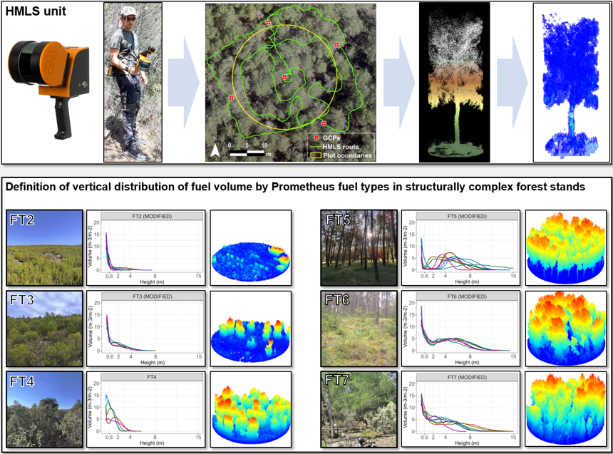
HMLS data were collected in the end of May 2023 using a GeoSLAM ZEB-Horizon unit (GeoSLAM Ltd., Ruddington, UK) (Figure 2a), capable of scanning 300,000 points per seconds with a maximum scan range of 100 m and 360º x 270º field of view. Scans began at the center of each plot, following by an inner circular scan at about 1 m from the plot center, and another outer circular scan at the plot boundaries, pointing towards the center of the plot. Next, a detail scan was performed within the plot in dense and shadowed areas to avoid occlusion problems, ending the scan at the starting point located at the plot center. An example of the route followed in one plot can be seen in Figure 2b. The scanning time for each plot was about 10–15 minutes. The interaction of the laser system with the vegetation produced very-high density three-dimensional point clouds, with an average point density for all plots of 63,148 points/m2 (detailed densities for each plot are shown in Table S1 of Supplementary Materials). Since the HMLS system did not incorporate an inertial measurement unit, data were collected in local coordinates (i.e., the center of the plot had the coordinates XY 0,0) and later georeferenced to a coordinate reference system. For this, 5 ground control points (GCPs) were set up in each plot before the start of the scans with the Leica Viva® GS15 CS10 GNSS. One GCP was placed in the center of the plot and the remaining four in each of the cardinal points of the plots boundaries (Figure 2b). During the scans, the HMLS remained at least 10 seconds static and at ground level on each GCP to record the local coordinates and then match it with the coordinates obtained from the GNSS in the same GCP. For data pre-processing, the proprietary software GeoSLAM Connect v.2.3.0 was used. It involved converting the scans into LAS files and georeferencing local coordinates to a coordinate reference system (EPSG: 25830 – ETRS89 / UTM zone 30N). For the latter, the `Stop and Go alignment´ tool was used, which allowed associating the local coordinates registered with the HMLS to the coordinates recorded with the GNSS on each GCP in the coordinate reference system. The mean georeferencing error for all plots was 0.161 m (detailed results are shown in Table S1 of Supplementary Materials).
2.3. Ground points classification
The georeferenced point clouds were classified into ground and non-ground points for the generation of Digital Elevation Models (DEMs) and heights normalization. This process is a key step for ensuring that subsequent analyses are accurate, given the very-high point cloud density of the HMLS data. For this, three different ground classification algorithms, commonly used in forestry, were tested: The `lasground´ algorithm of LasTools (Rapidlasso GmbH, Germany), the Multiscale Curvature Classification (MCC) algorithm [52], and the Cloth Simulation Filter (CSF) algorithm [53]. The software used for this purpose were ArcMap v.10.7.1 (ESRI, 2019) for LasTools, MCC-LiDAR v.2.1 [52] for MCC, and the lidR package [54,55] for R environment [56] for CSF. The classification could be applied without reducing the original point cloud densities in the cases of LasTools and CSF, but with MCC, point clouds had to be decimated to 1,000 points/m2 due to computational limitations. The points classified as ground by the three algorithms were used to generate DEMs with a spatial resolution of 0.20 m by TIN-to-raster interpolation method [57] using the `rasterize terrain´ function of the lidR package. After that, elevation values were extracted from the DEMs through random sampling of 2,000 points, and they were compared with each other to compute the mean height error for each algorithm. The DEMs from the algorithm with the lowest mean error were selected to normalize the heights of the point clouds. For this, the `normalize heights´ function of the lidR package was used. Finally, normalized points with negative height values or exceeding 40 m (i.e., outliers) were removed using the `filter poi´ function of lidR.
2.4. Voxelization and fuel load quantification
Estimation of fuel load was performed by calculating the volume of the normalized point clouds. For this purpose, a voxelization process was conducted, which has been reported as a well suited approach for estimating forest fuels (e.g., [58,59,60,61]) and allows simplifying the huge amount of data coming from ground-based LiDAR systems [62,63,64,65,66]. In doing so, the effect of uneven point distributions, many of which tend to be located closer to the sensor, is normalized [63,64]. The first step prior to the voxelization process was to consider the resolution of the voxels, so that they can accurately describe the heterogeneous structure and distribution of the fuel loads without loss of information. Considering the average point clouds densities, voxels were generated at 5 cm grid resolution using the VoxR package for R [64,67]. Prior voxelization, points considered as noise were filtered out using the Statistical Outliers Removal (SOR) filter available in the VoxR package. The SOR filter considers a point to be noise if it is at a distance to its nearest neighbors greater than the mean distance of the entire point cloud plus 1.5 times the standard deviation of other points [67]. As a result of voxelization, each plot was composed by a collection of filled and empty voxels in the XYZ space (Figure 3). Filled voxels indicated the presence of at least one point of the point cloud, while empty voxels denoted an absence of points.
The total volume for each plot in each 5 cm height stratum was computed as a sum of the filled voxels in each stratum multiplied by their size (Equation 1) [65]. In order to take into account, with a cautious approach, the measurement accuracy of the instrument, which is around 1–3 cm, for subsequent analyses, the first voxelized stratum (i.e., voxels between 0 and 5 cm of height) was not considered to ensure not working with returns that may belong to the ground and not to fuel. The volume of each height stratum was calculated in absolute (m3/m2) and relative (% of the total) terms. The total volume of fuel load was also calculated for each height threshold of the Prometheus model: below 0.60 m for the low shrub (LSh) stratum, between 0.60 – 2 m for the medium shrub (MSh) stratum, between 2 – 4 m for the high shrub (HSh) stratum, and above 4 m for the tree stratum (Tr) for quantifying the average fuel load for each fuel type.
Where `VOL´ is the total volume in absolute (m3/m2) and relative (% of the total) terms in the `s´ height stratum; and `VOX´ are the filled voxels in the `s´ height stratum.
3. Results
3.1. Visual analyses of the processed point clouds
A preliminary assessment of the differentiation capability between Prometheus fuel types was conducted through visual analysis of the point clouds. Figure 4 illustrates the structural heterogeneity of vegetation at the plot and transect scale by fuel type. It can be seen that the acquired and processed data successfully represents the vertical distribution of vegetation, even in the upper strata (e.g., canopies), which are further away from the ground, where data are acquired. The LSh, MSh, and HSh strata (i.e., shrub strata) are predominant in FT2, FT3, and FT4, respectively. In addition, some scattered larger shrubs or small trees can be found in FT2 and FT3 plots, while in FT4 there is a greater spatial continuity of tall shrubs. In FT5, the point cloud clearly represents the tree profile and the absence of understory. Continuity of vegetation can be observed between the lower and upper strata for the tree fuel types as in FT6, but less than in FT7, where the fuel reaches the maximum structural volume and the highest stand compactness.
3.2. Selection of the ground points classification algorithm
Figure 5 shows the results of the comparative analyses of the mean height error for each plot and between algorithms. Detailed results can be found in Table S2 of Supplementary Materials. There were few differences in the height values extracted from MCC and CSF (mean error = 4 cm, standard deviation = 4 cm), while in LasTools, the differences with the other two algorithms were slightly larger (LasTools–MCC: mean error = 19 cm, standard deviation = 28 cm; LasTools–CSF: mean error = 20 cm, standard deviation = 26 cm). Regarding the classification process, MCC took quite some time to process the decimated point cloud, while LasTools and CSF processed the complete point cloud in less time. Therefore, based on these results, the CSF algorithm was chosen as the most suitable for filtering and classifying the point clouds in ground and non-ground points in order to normalize the heights of the point clouds.
3.3. Definition of Prometheus fuel types
The vertical distribution of the fuel volume every 5 cm allowed defining specific distributions of the Prometheus fuel types for each forest plot (see Figures S1, S2, and S3 of Supplementary Materials), which enabled the identification of plots with incorrectly estimated fuel types in the field.
In general terms, the Prometheus shrub fuel types (FT2, FT3, and FT4) are characterized by a unimodal distribution, except some cases in FT4, with peaks in the LSh stratum and a gradual decrease in fuel towards the higher strata, almost disappearing in the MSh stratum (Figure 6). In FT2, the fuel is concentrated in the LSh stratum, and only few plots show a slight increase between 0.6 and 4 m, which can be explained by the presence of scattered low trees within those plots, but it does not affect the overall appearance of the distribution. In FT3, the decline in fuel load is not as abrupt as in FT2 in the LSh stratum but stabilizes in the MSh stratum before gradually decreasing down to the Tr stratum. The distribution of FT4 differs slightly from that of FT2 and FT3, as the peak can be found in both the LSh and MSh strata. Additionally, there is a higher volume of fuel in the MSh stratum. Some plots have also a bimodal distribution, with peaks in both the LSh and MSh strata. These distributions in FT4 suggest the continuity of the vertical fuel structure below 4 m, which is characteristic of this fuel type. According to these results, a total of 4 shrub-type plots with incorrectly estimated fuel types in the field were identified. One plot initially classified as FT2 (`vi40´) did not match the average distribution for this fuel type, as it had higher fuel volume in the MSh stratum and it aligned better with FT3. Thus, the ground-truth was changed to this fuel type. Additionally, three plots classified as FT3 (`vi17´, `zu30´, and `zu31´) were modified to FT2, as their volume distribution were characterized by an abrupt decrease in fuel from the MSh stratum, and fit better with the FT2 distributions. In the case of FT4 plots, no modifications were made.
Regarding the Prometheus tree fuel types, FT5 has a clearly distinctive distribution, while FT6 and FT7 distributions look fairly similar but with a slight nuance that sets them apart (Figure 7). FT5 exhibits a very clear bimodal distribution, with a main peak located in the LSh stratum and a secondary peak that can start in the HSh stratum and continue into the Tr stratum, or that starts directly in the Tr stratum, with very little fuel load volume in the MSh stratum. The distribution of FT6 shows a peak in the LSh stratum, followed by a decrease in the MSh stratum and then a small increase in the HSh stratum, ending in a gradual decrease from the Tr stratum. FT7 has a very similar distribution to FT6, except that the volume remains more stable during the MSh and HSh strata before decreasing from the Tr stratum, suggesting more volume in the intermediate strata and, thus, more vertical continuity of fuel load, which is characteristic of this type. These results show that the ground-truth was incorrectly identified in the field in 6 tree-type plots. Two plots initially identified as FT6 (`ay12´ and `ay49´) were changed to FT5 due to the distinctive bimodality of their distributions and the very low volume present in the MSh and HSh strata. Another plot identified as FT6 in the field (`ay31´) was changed to FT7, as it showed a consistent fuel volume between the LSh and MSh strata. Moreover, three plots originally labeled as FT7 (`ay06´, `ay19´, and `ay28´) were corrected to FT6, as their distributions exhibited a decrease in volume in the MSh stratum, indicating probable less vertical continuity of vegetation. Finally, it is necessary to highlight the case of a plot labeled as FT7 (`vi41´, which correspond to the pink line in the FT7 plots of Figure 7) that shows a distinctive signature compared to others of the same fuel type. This is a plot that could be on the border between FT4 and FT7, as there is a clear bimodality that could resemble that found in some FT4 plots. However, there is a significant amount of fuel load from the Tr stratum, and it does not decrease completely until approximately 8 meters, which may be excessive for a FT4 plot. Therefore, the ground-truth has not been modified, assuming that this is a FT7 plot with low tree height.
3.4. Quantification of Prometheus fuel load
The quantification of fuel load by Prometheus height strata allowed confirming the corrections made to the ground-truth in the 10 forest plots. The results presented below are grouped by the fuel types modified from the HMLS data and mentioned in the previous section. Figure 8 shows the fuel volume of each Prometheus shrub fuel types, where a generally progressive increase in the total volume is observed from FT2 to FT4: Volume is less than 250 m3/m2 in FT2, slightly over 250 m3/m2 in FT3 (except for one plot: `vi40´), and somewhat higher than 250 m3/m2 in FT4. The aforementioned plot `vi40´ was misclassified as FT2 in the field, and it is the only one among FT3 that does not exceed 250 m3/m2 of total volume. This suggests that this plot could be on the border between FT2 and FT3. However, the percentage of volume contained in the MSh and HSh strata in this plot is quite high (> 20%) and it resembles the percentages of FT3 plots more closely. Regarding the percentage of volume in each Prometheus stratum, a clear dominance of the LSh stratum is observed in FT2 (> 50% of total volume in all plots except for one), greater parity in FT3 but with more significant proportions in the two lower strata, and a predominance of the MSh stratum in FT4. As expected, the percentage of total volume in Tr stratum is almost negligible in the three shrub types. Only three FT2 plots have volume in the HSh and Tr strata, which are related to the small volume increments seen in these strata in Figure 5 and explained before. There is a higher volume percentage in the Tr stratum in FT3 plots, but they are still low values, while there is hardly any in FT4. Finally, it is worth noting that the volumes of the plots where the ground-truth was corrected (`vi17´, `vi40´, `zu30´, and `zu31´) fit quite well within their respective new groups.
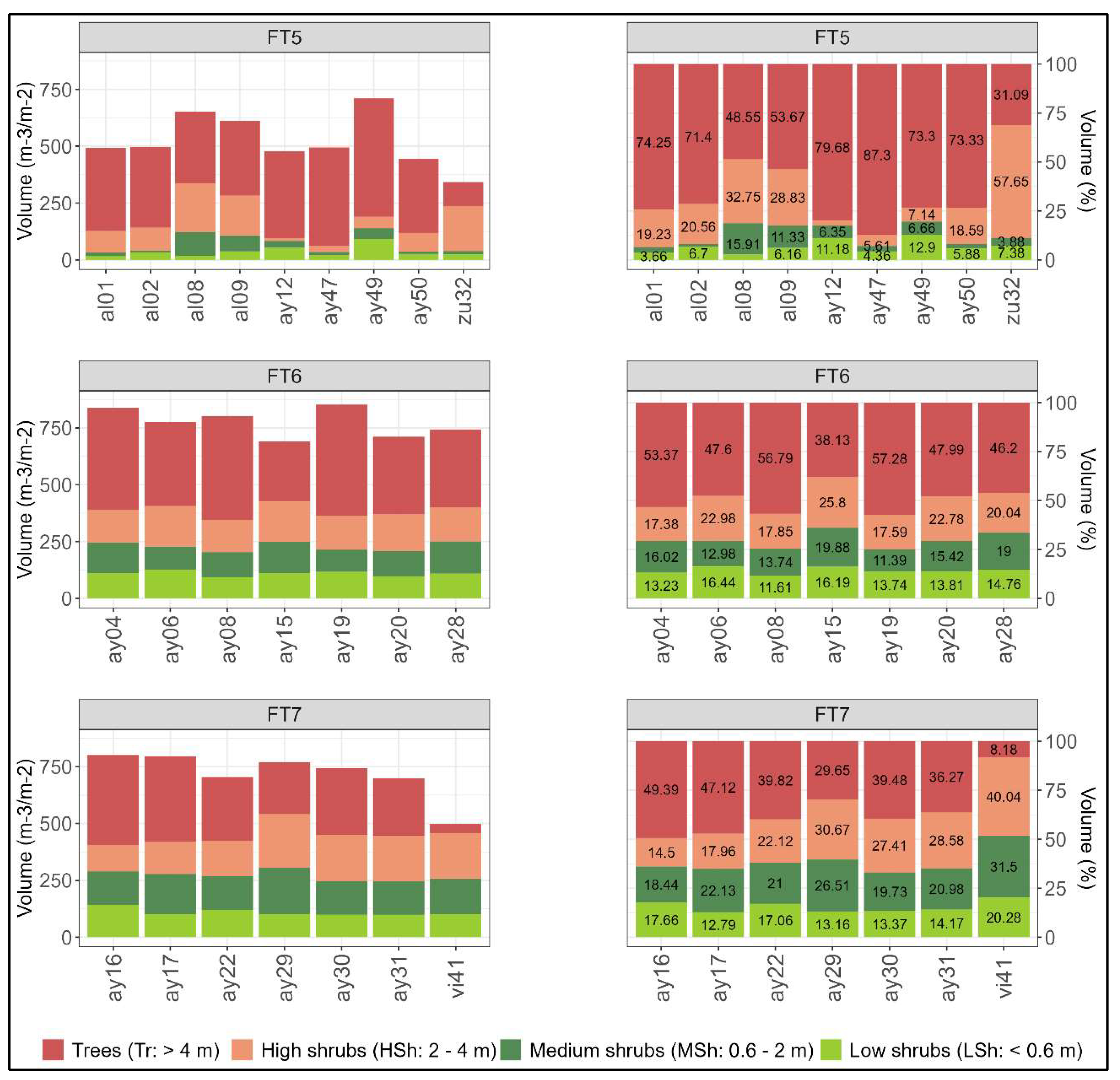
In the Prometheus tree fuel types, there is a lower volume of fuel load in FT5 (< 750 m3/m2) due to the absence of understory, and a slightly higher volume in FT6 plots compared to FT7 (Figure 9) due to a greater volume of tree canopies in the former. In general terms, the dominant stratum in these types is the Tr stratum, reaching the highest percentages in FT5 plots. FT7 plots have greater uniformity in the volume contained in each Prometheus stratum, although some plots show similar volume percentages in the MSh and HSh strata to others identified as FT6 (e.g., `ay16´ and `ay17´). This may be an indicator of the high complexity of the vertical fuel structure in both plot types. However, in FT6 plots there are no cases of volume percentages higher than 20% in the same plot in both MSh and HSh strata, while there are in most FT7 plots, suggesting a greater vertical continuity of fuel between strata in the latter. Regarding FT5, the amount of volume in the LSh and MSh strata is very low, and appreciable amounts are only found in plots `al08´, `al09´, `ay12´, and `ay49´. In the case of the former two, it is due to a higher percentage of MSh strata, although this percentage is not high. The latter two were labeled in the field as FT6 because they had a higher volume of fuel in the MSh stratum compared to other FT5 plots. However, their volume by Prometheus height strata seems to fit better in FT5, confirming the corrections made previously. Plot `zu32´ has the most distinctive volume distribution of all FT5 plots, as the dominant stratum is the HSh stratum, assuming that this is a FT5 plot with low tree height. On the other hand, the volume of plot `ay31´, whose fuel type was labeled as FT6 in the field, fits quite well as FT7. Plots `ay06´, `ay19´, and `ay28´, which transitioned from FT7 to FT6, also seem to fit better with their new type. Lastly, it is confirmed that plot `vi41´ is a `low FT7´ plot, since it has very little volume in the Tr stratum but a lot in the HSh stratum. Its distribution closely resembles FT4 plots, although with significantly more volume in the upper strata, so it might not be appropriate to label it as FT4.
4. Discussion
In the current context of increasing exposure to wildfires, it is necessary to develop plans to mitigate their negative effects on the environment. An effective step is to correctly identify the fuel types in the field to model accurately fire behavior in larger areas. However, forest stands are often structurally complex and present mixed features of several fuel types, especially in the Mediterranean region, making sometimes in situ estimation of fuels challenging. This study has relied on an HMLS system to address this challenge, since its ability to obtain detailed data on forest vertical and horizontal structure allows for a more precise characterization of vegetation and definition of Prometheus fuel types. Thanks to the large amount of data involved, the corrections made to incorrectly identified fuel types in the field were successful. Additionally, the proposed methodology, based on the use of an HMLS system, provides an efficient alternative for the estimation and correction of fuel types in forest environments. The results show that voxelization of the very-high density three-dimensional point clouds from the HMLS data allowed the identification of specific distributions of the vertical fuel volume for each Prometheus fuel type. The quantification of the fuel volume by Prometheus height strata validated the information provided by the distributions, and the fuel types of 10 plots were re-labeled to their closest fuel type.
CSF was the most suitable algorithm for the classification of the ground points. Filtering is a key process to normalize the heights and to ensure greatest accuracies in the subsequent voxelization and fuel volume estimation by height ranges. This algorithm has already been used in previous studies that have employed HMLS systems (e.g., [37,45]), as well as TLS systems (e.g., [62,68]) and other MLS systems (e.g., [44]). Results of the centimetric-scale voxelization (5 cm) appear to be adequate to better identify the vertical distribution of fuels and accurately estimate the Prometheus fuel types without loss of information on the structural complexity of the forest stands. Although voxel size will depend on research objectives and the quality of the data [64], several studies using ground-based LiDAR systems have employed small-sized voxels for volume estimation with satisfactory results. For instance, when using TLS, Lecigne et al. (2018) [64] noticed that smaller voxels were more suitable for capturing fine changes in tree features compared to larger voxel sizes, which is crucial when working in structurally complex environments such as Mediterranean forests. Yan et al. (2019) [69] generated voxels of 20 cm size for crown volume estimation from MLS-derived point cloud. Voxel sizes of 10 cm have also been used to estimate forest fuel characteristics with a TLS system [61] and stand structural features with a HMLS system [65]. In this study, the volume of fuel load has been calculated directly from the voxels, but it can also be estimated through indices derived from the voxels themselves. For instance, a voxel-derived index called PDI (Plant Diversity Index) was proposed by Puletti et al. (2021) [70], which relates the number of filled voxels to the total number of voxels within the same height stratum, resulting satisfactory in estimating the vertical distribution of fuel volume. Despite the small voxel size used for the voxelization and the very-high density of the point clouds, the process was relatively fast and allowed for more efficient management of the vast amount of data collected with the HMLS. In this regard, voxels allow for the removal of some unwanted effects typical of ground-based LiDAR systems, such as occlusion or differences in point cloud densities, which can introduce bias in the characterization of fuel structure. This process of discretizing point clouds also helps in monitoring forest changes over different time periods [71,72,73], which could be valuable for detecting progressive changes in the fuel types over time due to natural vegetation growth. In this sense, working directly with the point cloud would have been computationally more demanding, as the extraction of structural metrics to estimate the distribution and density of forest structure is typically done at the pixel or plot level. Thus, this study proposes a simpler methodology for better defining fuel types and correct those that were incorrectly estimated in the field.
Among the various platforms of ground-based LiDAR systems, this study has used an HMLS in a novel application in forestry. Overall, the results of modifications for incorrectly estimated fuel types in the field are satisfactory and highlights the value of HMLS systems for quantifying the volume of fuel load and define precisely the Prometheus fuel types. However, some limitations have been observed stemming from the estimation of fuel volume in quantitative units (m3/m2). For instance, some FT6 and FT7 plots exhibited a very similar vertical distribution of fuel (Figure 9) that may create confusion and not allow to correctly differentiate each type, even when working at centimetric scales, as in this study. In addition, the voxels were computed for the entire point cloud without distinguishing between the different nature to which the points refer. The voxels did not differentiate which part of the vegetation are foliage, branches, trunks, or bark, which is relevant in relation to wildfires. In this regard, some studies have attempted to categorize the voxels according to their class in order to improve fuel quantification (e.g., [58,59]). Nevertheless, this can be a complex task in forest environments of very-high structural heterogeneity, where different fuel classes are intermingled. Another limitation is that it is not possible to differentiate between live and dead fuel from the raw point cloud data. Some HMLS systems allow the collection of data in combination with RGB images, which could help in distinguishing between both types of fuels, although the processing could be time- and resource-intensive, but it would allow for improved fuel characterization and more accurate fire spread modeling. Despite these limitations, the HMLS system has allowed the identification of plots with incorrectly estimated fuel types in the field and correct them to their closest type. The observed confusions align with previous studies, which also reported such inaccuracies (e.g., [21,22,24,25]). Main confusion between fuel types may occur due to incorrect estimation of the shrub or understory volume. In shrub fuel types, it determines the maximum height, while in tree fuel types, it defines the degree of vertical continuity between the understory and the canopies. Although ground-based LiDAR systems have been shown to better identify understory fuel than other systems [74,75], the use of other remote sensing platforms could help to improve the estimation of understory fuels. For instance, Hillman et al. (2021) [62] found that LiDAR sensors mounted on unmanned aerial vehicles (LiDAR UAVs) were capable of estimating understory fuels as accurately as a TLS system in a dry sclerophyll forest. Instead, Hyyppä et al. (2020a) [43] demonstrated that above-canopy LiDAR UAVs do not perform well in identifying forest understory attributes, but that under-canopy LiDAR UAVs can achieve similar performance to ground-based LiDAR systems [43,76]. Therefore, LiDAR UAVs could be considered as good alternatives to identify fuel types, as they are also capable of acquiring data in larger areas, but may be subject to more restrictive regulations and not very operative in dense and complex forests. HMLS data can also be obtained over large areas, but require more time and effort, and some forest plots may be inaccessible due to their extremely high vegetation density, which can be common in Mediterranean forests. In spite of this, HMLS systems allow for a larger scanning area than TLS [40], provide free mobility within the forest, and data can be georeferenced indirectly with GCPs or directly if the system is equipped with an inertial measurement unit. Therefore, based on our findings, HMLS systems should be considered promising tools to improve field fuel load estimation, which will lead to better forest fuels modeling and, consequently, help in forest fire prevention and mitigation plans.
5. Conclusions
Knowing the spatial distribution of forest fuels is a crucial step to understand the fire behavior in a hypothetical forest fire. In this sense, ground-based LiDAR systems can provide highly detailed information about the vertical distribution of fuel load in the forest at an exceptional detail, which can be of great interest to improve the field estimation of fuel types. The results of this study conclude that HMLS systems are capable of detecting fuel load at centimetric-scale height strata in heterogeneous forest plots. With this information, it is possible to determine the fuel type to which the plot belongs, even when there is a mixture of characteristics of different fuel types, a quite common situation in Mediterranean forest environments. This study focused on the Prometheus model, but the approach could be applied to other relevant fire models. In this way, an improved identification of the fuel types can enhance the ground-truth of classification models, enabling more accurate modeling of fire behavior in larger areas. This ultimately contributes to improve the prevention and mitigation of wildfires over the territory.
Supplementary Materials
The following supporting information can be downloaded at: Preprints.org, Figure S1: Vertical distribution of the fuel volume of each forest plot every 5 cm (1/3); Figure S2: Vertical distribution of the fuel volume of each forest plot every 5 cm (2/3); Figure S3: Vertical distribution of the fuel volume of each forest plot every 5 cm (3/3); Table S1: Name, location, point cloud density, and mean georeferenced error of the forest plots. Plot `zu38´ have a 10 m circular radius; Table S2: Mean height error (in meters) between the three ground classification algorithms tested in the study for each plot.
Author Contributions
Conceptualization, R.H.; M.T.L. and J.d.l.R.; methodology, R.H.; M.T.L. and J.d.l.R.; software, R.H.; validation, R.H.; M.T.L. and J.d.l.R.; formal analysis, R.H.; investigation, R.H.; M.T.L. and J.d.l.R.; data curation, R.H.; writing—original draft preparation, R.H.; writing—review and editing, R.H.; M.T.L. and J.d.l.R. All authors have read and agreed to the published version of the manuscript.
Funding
This work was supported by the Spanish Ministry of Science, Innovation, and Universities through an FPU predoctoral contract granted to R.H. [FPU18/05027]; by the Government of Aragón [Geoforest S51_23R co-financed with FEDER `Construyendo Europa desde Aragón´]; and by the University Institute for Research in Environmental Sciences of Aragón (IUCA) of the University of Zaragoza, for covering the cost of renting the GeoSLAM ZEB-Horizon HMLS unit and the GeoSLAM Connect v.2.3.0 software.
Data Availability Statement
Dataset are available on request.
Acknowledgments
The authors would like to thank Grafinta S.A. (Av. Filipinas 46, 28003 Madrid, Spain) for providing the GeoSLAM ZEB-Horizon HMLS unit and the GeoSLAM Connect v.2.3.0 software, as well as for their continuous support and guidance, especially David Cruz. The authors also thank Dr. Darío Domingo for his support in the field work.
Conflicts of Interest
The authors declare no conflict of interest.
References
- Bowman, D.M.J.S.; Balch, J.K.; Artaxo, P.; Bond, W.J.; Carlson, J.M.; Cochrane, M.A.; D'Antonio, C.M.; Defries, R.S.; Doyle, J.C.; Harrison, S.P.; Johnston, F.H.; Keeley, J.E.; Krawchuk, M.A.; Kull, C.A.; Marston, J.B.; Moritz, M.A.; Prentice, I.C.; Roos, C.I.; Scott, A.C.; Swetnam, T.W.; van der Werf, G.R.; Pyne, S.J. Fire in the Earth System. Science 2019, 324, 5926. [Google Scholar] [CrossRef]
- Pausas, J.G.; Keeley, J.E. A burning story: The role of fire in the history of life. Bioscience 2009, 59, 593–601. [Google Scholar] [CrossRef]
- Nocentini, S.; Coll, L. Mediterranean forests: Human use and complex adaptive systems. In Managing forests as complex adaptive systems. Building resilience to the challenge of global change; Messier, C.; Puettmann, K.J.; Coates, K.D.; Eds.; Routledge, London, UK, 2013, pp. 214–243.
- Jones, M.W.; Abatzoglou, J.T.; Veraverbeke, S.; Andela, N.; Lasslop, G.; Forkel, M.; Smith, A.J.P.; Burton, C.; Betts, R.A.; van der Werf, G.R.; Sitch, S.; Canadell, J.G.; Santín, C.; Kolden, C.; Doerr, S.H.; Le Quéré, C. Global and regional trends and drivers of fire under climate change. Rev. Geophys. 2022, 60, e2020RG000726. [Google Scholar] [CrossRef]
- Rovithakis, A.; Grillakis, M.G.; Seiradakis, K.D.; Giannakopoulos, C.; Karali, A.; Field, R.; Lazaridis, M.; Voulgarakis, A. Future climate change impact on wildfire danger over the Mediterranean: The case of Greece. Environ. Res. Lett. 2022, 17, 045022. [Google Scholar] [CrossRef]
- Ruffault, J.; Curt, T.; Moron, V.; Trigo, R.M.; Mouillot, F.; Koutsias, N.; Pimont, F.; Martin-StPaul, N.; Barbero, R.; Dupuy, J.L.; Russo, A.; Belhadj-Khedher, C. Increased likelihood of heat-induced large wildfires in the Mediterranean Basin. Sci. Rep. 10 2020, 13790. [Google Scholar] [CrossRef]
- Varela, V.; Vlachogiannis, D.; Sfetsos, A.; Karozis, S.; Politi, N.; Giroud, F. Projection of forest fire danger due to climate change in the French Mediterranean region. Sustainability 2019, 11, 4284. [Google Scholar] [CrossRef]
- Ascoli, D.; Moris, J.V.; Marchetti, M.; Sallustio, L. Land use change towards forests and wooded land correlates with large and frequent wildfires in Italy. Ann. Silvic. Res. 2021, 46, 177–188. [Google Scholar] [CrossRef]
- Koutsias, N.; Martínez-Fernández, J.; Allgöwer, B. Do factors causing wildfires vary in space? Evidence from Geographically Weighted Regression. GIScience Remote Sens. 2013, 47, 221–240. [Google Scholar] [CrossRef]
- Moreno, M.V.; Conedera, M.; Chuvieco, E.; Pezzatti, G.B. Fire regime changes and major driving forces in Spain from 1968 to 2010. Environ. Sci. Policy 2014, 37, 11–22. [Google Scholar] [CrossRef]
- Chas-Amil, M.L.; Touza, J.; García-Martínez, E. Forest fires in the wildland-urban interface. A spatial analysis of forest fragmentation and human impacts. Appl. Geogr. 2013, 43, 127–137. [Google Scholar] [CrossRef]
- Ganteaume, A.; Barbero, R.; Jappiot, M.; Maillé, E. Understanding future changes to fires in southern Europe and their impacts on the wildland-urban interface. J. Saf. Sci. Resil. 2021, 2, 20–29. [Google Scholar] [CrossRef]
- Godoy, M.M.; Martinuzzi, S.; Masera, P.; Defossé. G.E. Forty years of Wildland Urban Interface growth and its relation with wildfires in Central-Western Chubut, Argentina. Front. For. Glob. Change 2022, 5. [Google Scholar] [CrossRef]
- Turco, M.; Llaset, M.C.; von Hardenberg, J.; Provenzale, A. Climate change impacts on wildfires in a Mediterranean environment. Clim. Change 2014, 125, 369–380. [Google Scholar] [CrossRef]
- Ferraz, A.; Saatchi, S.; Mallet, C.; Meyer, V. LiDAR detection of individual tree size in tropical forests. Remote Sens. Environ. 2016, 183, 318–333. [Google Scholar] [CrossRef]
- Huesca, M.; Riaño, D.; Ustin, S.L. Spectral mapping methods applied to LiDAR data. Application to fuel type mapping. Int. J. Appl. Earth Obs. Geoinf. 2019, 74, 159–168. [Google Scholar] [CrossRef]
- Rothermel, C. A mathematical model for predicting fire spread in wildland fuels. Research Papers, U: Ogden, UT.
- Albini, F. Estimating wildfire behavior and effects. USDA Forest Service. Intermountain Forest and Range Experiment Station. General Technical Report, 1976; INT-30, 92. [Google Scholar]
- Prometheus. Management techniques for optimization of suppression and minimization of wildfires effects. System Validation. European Commission, DG XII, ENVIR & CLIMATE, Contract Number ENV4-CT98-0716. European Commission, Luxembourg. 1999.
- Arroyo, L.A.; Pascual, C.; Manzanera, J.A. Fire models and methods to map fuel types: The role of remote sensing. For. Ecol. Manag. 2008, 256, 1239–1252. [Google Scholar] [CrossRef]
- Arroyo, L.A.; Healey, S.P.; Cohen, W.B.; Cocero, D.; Manzanera, J.A. Using object-oriented classification and high-resolution imagery to map fuel types in a Mediterranean region. J. Geophys. Res. 2006, 111, G04S04. [Google Scholar] [CrossRef]
- Domingo, D.; de la Riva, J.; Lamelas, M.T.; García-Martín, A.; Ibarra, P.; Echeverría, M.T.; Hoffrén, R. Fuel type classification using airborne laser scanning and Sentinel-2 data in Mediterranean forest affected by wildfires. Remote Sens. 2020, 12, 1–22. [Google Scholar] [CrossRef]
- Hoffrén, R.; Lamelas, M.T.; de la Riva, J.; Domingo, D.; Montealegre, A.L.; García-Martín, A.; Revilla, S. Assessing GEDI-NASA system for forest fuels classification using machine learning techniques. Int. J. Appl. Earth. Obs. Geoinf. 2023, 116, 103175. [Google Scholar] [CrossRef]
- Lasaponara, R.; Lanorte, A.; Pignatti, S. Characterization and mapping of fuel types for the Mediterranean ecosystems of Pollino National Park in southern Italy by using hyperspectral MIVIS data. Earth Interact. 2005, 10, 1–11. [Google Scholar] [CrossRef]
- García, M.; Riaño, D.; Chuvieco, E.; Salas, J.; Danson, F.M. Multispectral and LiDAR data fusion for fuel type mapping using Support Vector Machine and decision rules. Remote Sens. Environ. 2011, 115, 1369–1379. [Google Scholar] [CrossRef]
- Hoffrén, R.; Lamelas, M.T.; de la Riva, J. UAV-derived photogrammetric point clouds and multispectral indices for fuel estimation in Mediterranean forests. Remote Sens. Appl.: Soc. Environ. 2023, 31, 100997. [Google Scholar] [CrossRef]
- Revilla, S.; Lamelas, M.T.; Domingo, D.; de la Riva, J.; Montorio, R.; Montealegre, A.L.; García-Martín, A. Assessing the potential of the DART model to discrete return LiDAR simulation – Application to fuel type mapping. Remote Sens. 2021, 13, 1–21. [Google Scholar] [CrossRef]
- Åkerblom, M.; Kaitaniemi, P. Terrestrial laser scanning: A new standard of forest measuring and modelling? Ann. Bot. 2021, 128, 653–662. [Google Scholar] [CrossRef]
- Burt, A.; Disney, M.I.; Raumonen, P.; Armston, J.; Calders, K.; Lewis, P. Rapid characterization of forest structure from TLS and 3D modelling. In Proceedings of the 2013 IEEE International Geoscience and Remote Sensing Symposium – IGARSS 2013, Melbourne, VIC, Australia; pp. 3387–3390. [CrossRef]
- Liang, X.; Kankare, V.; Hyyppä, J.; Wang, Y.; Kukko, A.; Haggrén, H.; Yu, X.; Kaartinen, H.; Jaakkola, A.; Guan, F.; Holopainen, M.; Vastaranta, M. Terrestrial laser scanning in forest inventories. ISPRS J. Photogramm. Remote Sens. 2016, 115, 63–77. [Google Scholar] [CrossRef]
- Olofsson, K.; Holmgren, J. Single tree stem profile detection using terrestrial laser scanner data, flatness saliency features and curvature properties. Forests 2016, 7, 207. [Google Scholar] [CrossRef]
- Ritter, T.; Schwarz, M.; Tockner, A.; Leisch, F.; Nothdurft, A. Automatic mapping of forest stands based on three-dimensional point clouds derived from terrestrial laser-scanning. Forests 2017, 8, 265. [Google Scholar] [CrossRef]
- Rowell, E.; Seielstad, C. Characterizing grass, litter, and shrub fuels in longleaf pine forest pre- and post-fire using terrestrial LiDAR. Proceedings of SilviLaser 2012. SL2012-166 (19 09 2012).
- Chen, Y.; Zhu, X.; Yebra, M.; Harris, S.; Tapper, N. Strata-based forest fuel classification for wild fire hazard assessment using terrestrial LiDAR. J. Appl. Remote Sens. 2016, 10, 046025. [Google Scholar] [CrossRef]
- Loudermilk, E.L.; Pokwsinski, S.; Hawley, C.M.; Maxwell, A.; Gallagher, M.R.; Skowronski, N.S.; Hudak, A.T.; Hoffman, C.; Hiers, J.K. Terrestrial laser scan metrics predict surface vegetation biomass and consumption in a frequently burned southeastern U.S. ecosystem. Fire 2023, 6, 151. [Google Scholar] [CrossRef]
- Maxwell, A.E.; Gallagher, M.R.; Minicuci, N.; Bester, M.S.; Loudermilk, E.L.; Pokswinski, S.M.; Skowronski, N.S. Impact of reference data sampling density for estimating plot-level shrub heights using terrestrial laser scanning data. Fire 2023, 6, 98. [Google Scholar] [CrossRef]
- Donager, J.J.; Sánchez-Meador, A.J.; Blackburn, R.C. Adjudicating perspectives on forest structure: How do airborne, terrestrial, and mobile LiDAR-derived estimates compare? Remote Sens. 2021, 13, 2297. [Google Scholar] [CrossRef]
- Yrttimaa, T.; Saarinen, N.; Kankare, V.; Hynynen, J.; Huuskonen, S.; Holopainen, M.; Hyyppä, J.; Vastaranta, M. Performance of terrestrial laser scanning to characterize managed Scots pine (Pinus sylvestris L.) stands is dependent on forest structural variation. ISPRS J. Photogramm. Remote Sens. 2020, 168, 277–287. [Google Scholar] [CrossRef]
- Crespo-Peremarch, P.; Torralba, J.; Carbonell-Rivera, J.P.; Ruiz, L.A. Comparing the generation of DTM in a forest ecosystem using TLS, ALS and UAV-DAP, and different software tools. Int. Arch. Photogramm. Remote Sens. Spatial Inf. Sci. 2020, XLIII-B3-2020, 575–582. [Google Scholar] [CrossRef]
- Bauwens, S.; Bartholomeus, H.; Calders, K.; Lejeune, P. Forest inventory with terrestrial LiDAR: A comparison of static and hand-held mobile laser scanning. Forests 2016, 7, 127. [Google Scholar] [CrossRef]
- Fol, C.R.; Kükenbrink, D.; Rehush, N.; Murtiyoso, A.; Griess, V.C. Evaluating state-of-the-art 3D scanning methods for stem-level biodiversity inventories in forests. Int. J. Appl. Earth Obs. Geoinf. 2023, 122, 103396. [Google Scholar] [CrossRef]
- Gülci, S.; Yurtseven, H.; Akay, A.O.; Akgul, M. Measuring tree diameter using a LiDAR-equipped smartphone: A comparison of smartphone- and caliper-based DBH. Environ. Monit. Assess. 2023, 195, 678. [Google Scholar] [CrossRef]
- Hyyppä, E.; Yu, X.; Kaartinen, H.; Hakala, T.; Kukko, A.; Vastaranta, M.; Hyyppä, J. Comparison of backpack, handheld, under-canopy UAV, and above-canopy UAV laser scanning for field reference data collection in boreal forests. Remote Sens. 2020, 12, 3327. [Google Scholar] [CrossRef]
- de Paula Pires, R.; Olofsson, K.; Persson, H.J.; Lindberg, E.; Holmgren, J. Individual tree detection and estimation of stem attributes with mobile laser scanning along boreal forests roads. ISPRS J. Photogramm. Remote Sens. 2022, 187, 211–224. [Google Scholar] [CrossRef]
- Gollob, C.; Ritter, T.; Nothdurft, A. Forest inventory with long range and high-speed personal laser scanning (PLS) and simultaneous localization and mapping (SLAM) technology. Remote Sens. 2020, 12, 1509. [Google Scholar] [CrossRef]
- Solares-Canal, A.; Alonso, L.; Picos, J.; Armesto, J. Automatic tree detection and attribute characterization using portable terrestrial LiDAR. Trees 2023, 37, 963–979. [Google Scholar] [CrossRef]
- Tupinambá-Simões, F.; Pascual, A.; Guerra-Hernández, J.; Ordóñez, C.; de Conto, T.; Bravo, F. Assessing the performance of a handheld laser scanning system for individual tree mapping – A Mixed forests showcase in Spain. Remote Sens. 2023, 15, 1169. [Google Scholar] [CrossRef]
- Forbes, B.; Reilly, S.; Clark, M.; Ferrell, R.; Kelly, A.; Krause, P.; Matley, C.; O'Neil, M.; Villasenor, M.; Disney, M.I.; Wilkes, P.; Bentley, L.P. Comparing remote sensing and field-based approaches to estimate ladder fuels and predict wildfire burn severity. Front. For. Glob. Change 2022, 5. [Google Scholar] [CrossRef]
- Post, A.J. Using handheld mobile laser scanning to quantify fine-scale surface fuels and detect changes post-disturbance in northern California forests. Diss. Sonoma State University 2022. Available online: https://scholarworks.calstate.edu/downloads/t435gm64s.
- Coskuner, K.A.; Vatandaslar, C.; Ozturk, M.; Harman, I.; Bilgili, E.; Karahalil, U.; Berber, T.; Gormus, E.T. Estimating Mediterranean stand fuel characteristics using handheld mobile laser scanning technology. Int. J. Wildland Fire 2023, 32, 1347–1363. [Google Scholar] [CrossRef]
- Cuadrat, J.M.; Saz, M.A.; Vicente, S.M.
- Evans, J.S.; Hudak, A.T. A multiscale curvature algorithm for classifying discrete return LiDAR in forested environments. IEEE Trans. Geosci. Remote Sens. 2007, 45, 1029–1038. [Google Scholar] [CrossRef]
- Zhang, W.; Qi, J.; Wan, P.; Wang, H.; Xie, D.; Wang, X.; Yan, G. An easy-to-use airborne LiDAR data filtering method based on cloth simulation. Remote Sens. 2016, 8, 501. [Google Scholar] [CrossRef]
- Roussel, J.R.; Auty, D.; Coops, N.C.; Tompalski, P.; Goodboy, T.R.H.; Sánchez-Meador, A.; Bourdon, J.F.; de Boissieu, F.; Achim, A. 'lidR': An R package for analysis of Airborne Laser Scanning (ALS) data. Remote Sens. Environ. 2020, 251, 112061. [Google Scholar] [CrossRef]
- Roussel, J.R.; Auty, D. Airborne LiDAR data manipulation and visualization for forestry applications. R package version 4.0.1, 2022. Available online: https://cran.r-project.org/package=lidR.
- R Core Team. R: A language and environment for statistical computing. R Foundation for Statistical Computing, Vienna, Austria, 2022. Available online: https://www.R-project.org.
- Renslow, M. Manual of Airborne Topographic LiDAR; ASPRS: Bethesda, MD, USA, 2013; ISBN 978-1570830976. [Google Scholar]
- Barton, J.; Gorte, B.; Eusuf, M.S.R.S.; Zlatanova, S. A voxel-based method to estimate near-surface and elevated fuel from dense LiDAR point cloud for hazard reduction burning. ISPRS Ann. Photogramm. Remote Sens. Spatial Inf. Sci. 2020, VI-3/W1-2020, 3–10. Available online: https://isprs-annals.copernicus.org/articles/VI-3-W1-2020/3/2020/. [CrossRef]
- Eusuf, M.S.R.S.; Barton, J.; Gorte, B.; Zlatanova, S. (2020). Volume estimation of fuel load for hazard reduction burning: First results to a voxel approach. ISPRS Ann. Photogramm. Remote Sens. Spatial Inf. Sci. 2020, VI-3/W1-2020, 3–10. [Google Scholar] [CrossRef]
- Marcozzi, A.A.; Johnson, J.V.; Parsons, R.A.; Flanary, S.J.; Seielstad, C.A.; Downs, J.Z. Application of LiDAR derived fuel cells to wildfire modeling at laboratory scale. Fire 2023, 6, 394. [Google Scholar] [CrossRef]
- Rowell, E.; Loudermilk, E.L.; Hawley, C.; Pokswinski, S.; Seielstad, C.; Queen, L.; O'Brien, J.J.; Hudak, A.T.; Goodrick, S.; Hiers, J.K. Coupling terrestrial laser scanning with 3D fuel biomass sampling for advancing wildland fuels characterization. For. Ecol. Manag. 2020, 462, 117945. [Google Scholar] [CrossRef]
- Hillman, S.; Wallace, L.; Lucieer, A.; Reinke, K.; Turner, D.; Jones, S. A comparison of terrestrial and UAS sensors for measuring fuel hazard in a dry sclerophyll forest. Int. J. Appl. Earth Obs. Geoinf. 2021, 95, 102261. [Google Scholar] [CrossRef]
- Kato, A.; Watanabe, M.; Morgenroth, J.; Gomez, C. Field tree measurement using terrestrial laser for radar remote sensing. Proceedings of Asia-Pacific Conference on Synthetic Aperture Radar (APSAR), Asia-Pacific Conference, Japan, 2013., 119–121. Tsukuba.
- Lecigne, B.; Delagrange, S.; Messier, C. Exploring trees in three dimensions: VoxR, a novel voxel-based R package dedicated to analysing the complex arrangement of tree crowns. Ann. Bot. 2018, 121, 589–601. [Google Scholar] [CrossRef]
- Martínez-Rodrigo, R.; Gómez, C.; Toraño-Caicoya, A.; Bohnhorst, L.; Uhl, E.; Águeda, B. Stand structural characteristics derived from combined TLS and Landsat data support predictions of mushroom yields in Mediterranean forest. Remote Sens. 2022, 14, 5025. [Google Scholar] [CrossRef]
- Popescu, S.C.; Zhao, K. A voxel-based LiDAR method for estimating crown base height for deciduous and pine trees. Remote Sens. Environ. 2008, 112, 767–781. [Google Scholar] [CrossRef]
- Lecigne, B. 'VoxR': Trees geometry and morphology from unstructured TLS data. R package version 1.0.0, 2020. Available online: https://cran.r-project.org/package=VoxR.
- Panagiotidis, D.; Abdollahnejad, A.; Slavik, M. Assessment of stem volume on plots using terrestrial laser scanner: a precision forestry application. Sensors 2021, 21, 301. [Google Scholar] [CrossRef]
- Yan, Z.; Liu, R.; Cheng, L.; Zhou, X.; Ruan, X.; Xiao, Y. A concave hull methodology for calculating the crown volume of individual trees based on vehicle-borne LiDAR data. Remote Sens. 2019, 11, 623. [Google Scholar] [CrossRef]
- Puletti, N.; Galluzzi, M.; Grotti, M.; Ferrara, C. Characterizing subcanopy structure of Mediterranean forests by terrestrial laser scanning data. Remote Sens. Appl.: Soc. Environ. 2021, 24, 100620. [Google Scholar] [CrossRef]
- McCarley, T.R.; Kolden, C.A.; Vaillant, N.M.; Hudak, A.T.; Smith, A.M.S.; Wing, B.M.; Kellogg, B.S.; Kreitler, J. Multi-temporal LiDAR and Landsat quantification of fire-induced changes to forest structure. Remote Sens. Environ. 2017, 191, 419–432. [Google Scholar] [CrossRef]
- Srinivasan, S.; Popescu, S.C.; Eriksson, M.; Sheridan, R.D.; Ku, N.W. Multi-temporal terrestrial laser scanning for modeling tree biomass change. For. Ecol. Manag. 2014, 318, 304–317. [Google Scholar] [CrossRef]
- Zhao, K.; Suárez, J.C.; García, M.; Hu, T.; Wang, C.; Londo, A. Utility of multitemporal LiDAR for forest and carbon monitoring: Tree growth, biomass dynamics, and carbon flux. Remote Sens. Environ. 2018, 204, 883–897. [Google Scholar] [CrossRef]
- Arkin, J.; Coops, N.C.; Daniels, L.D.; Plowright, A. Canopy and surface fuel estimations using RPAS and ground-based point clouds. Forestry: An International Journal of Forest Research 2023, cpad020. [Google Scholar] [CrossRef]
- Beland, M.; Parker, G.; Sparrow, B.; Harding, D.; Chasmer, L.; Phinn, S.; Antonarakis, A.; Strahler, A. On promoting the use of LiDAR systems in forest ecosystem research. For. Ecol. Manag. 2019, 450, 117484. [Google Scholar] [CrossRef]
- Hyyppä, E.; Hyyppä, J.; Hakala, T.; Kukko, A.; Wulder, M.A.; White, J.C.; Pyöräla, J.; Yu, X.; Wang, Y.; Virtanen, J.P.; Pohjavirta, O.; Liang, X.; Holopainen, M.; Kaartinen, H. Under-canopy UAV laser scanning for accurate forest field measurements. ISPRS J. Photogramm Remote Sens. 2020, 164, 41–60. [Google Scholar] [CrossRef]
Figure 1.
Study area, location of the 43 forest plots, and detailed photo of 6
plots, one for each Prometheus fuel type considered in the study. Coordinate
reference system of the main map: EPSG: 25830 – ETRS89 / UTM zone 30N.
Figure 1.
Study area, location of the 43 forest plots, and detailed photo of 6
plots, one for each Prometheus fuel type considered in the study. Coordinate
reference system of the main map: EPSG: 25830 – ETRS89 / UTM zone 30N.
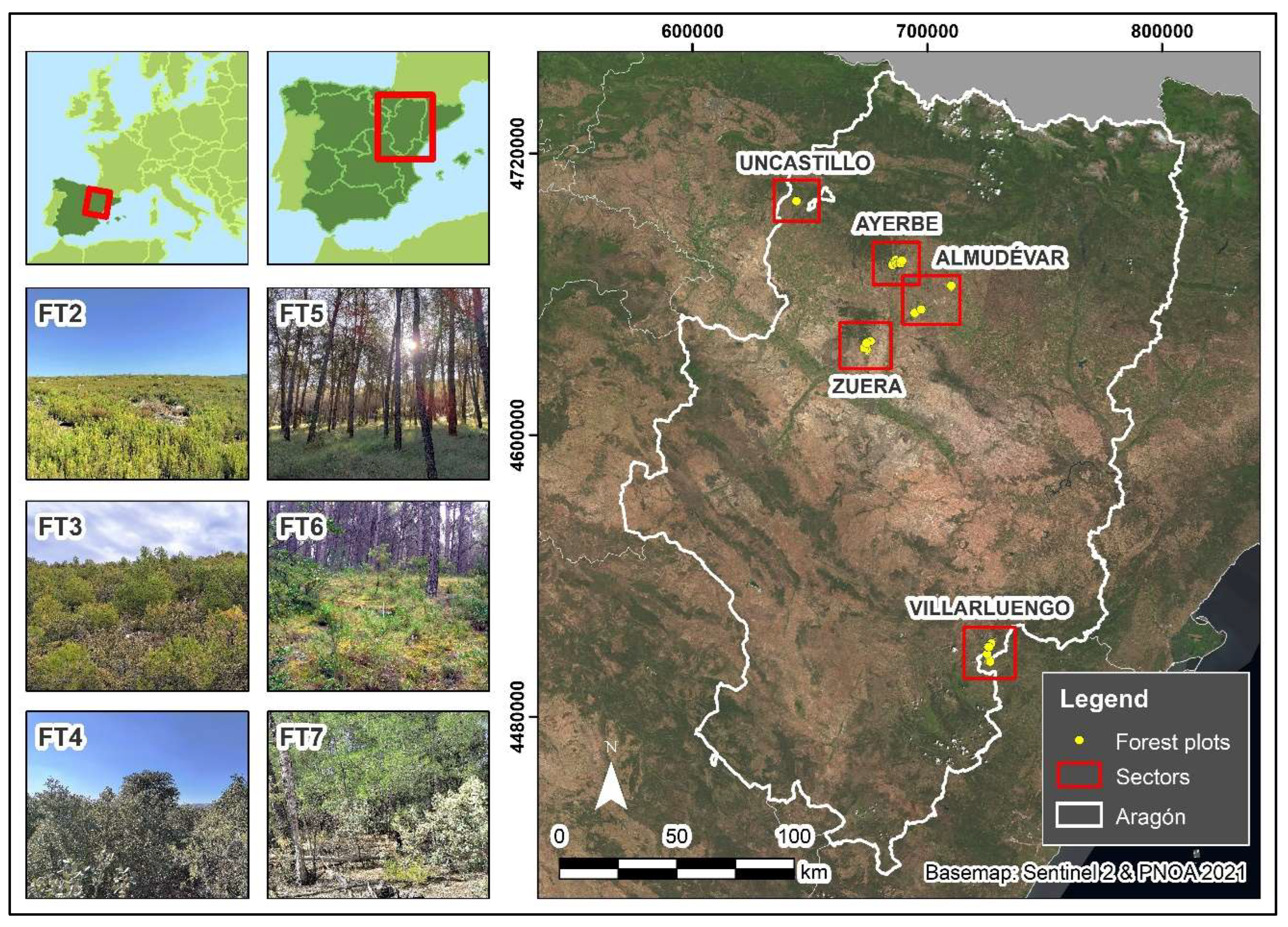
Figure 2.
(a) HMLS unit used in the study: GeoSLAM ZEB-Horizon (GeoSLAM Ltd., Ruddington, UK); (b) Example of the location of the 5 GCPs and the route followed to obtain the data in the plot `al09´.
Figure 2.
(a) HMLS unit used in the study: GeoSLAM ZEB-Horizon (GeoSLAM Ltd., Ruddington, UK); (b) Example of the location of the 5 GCPs and the route followed to obtain the data in the plot `al09´.
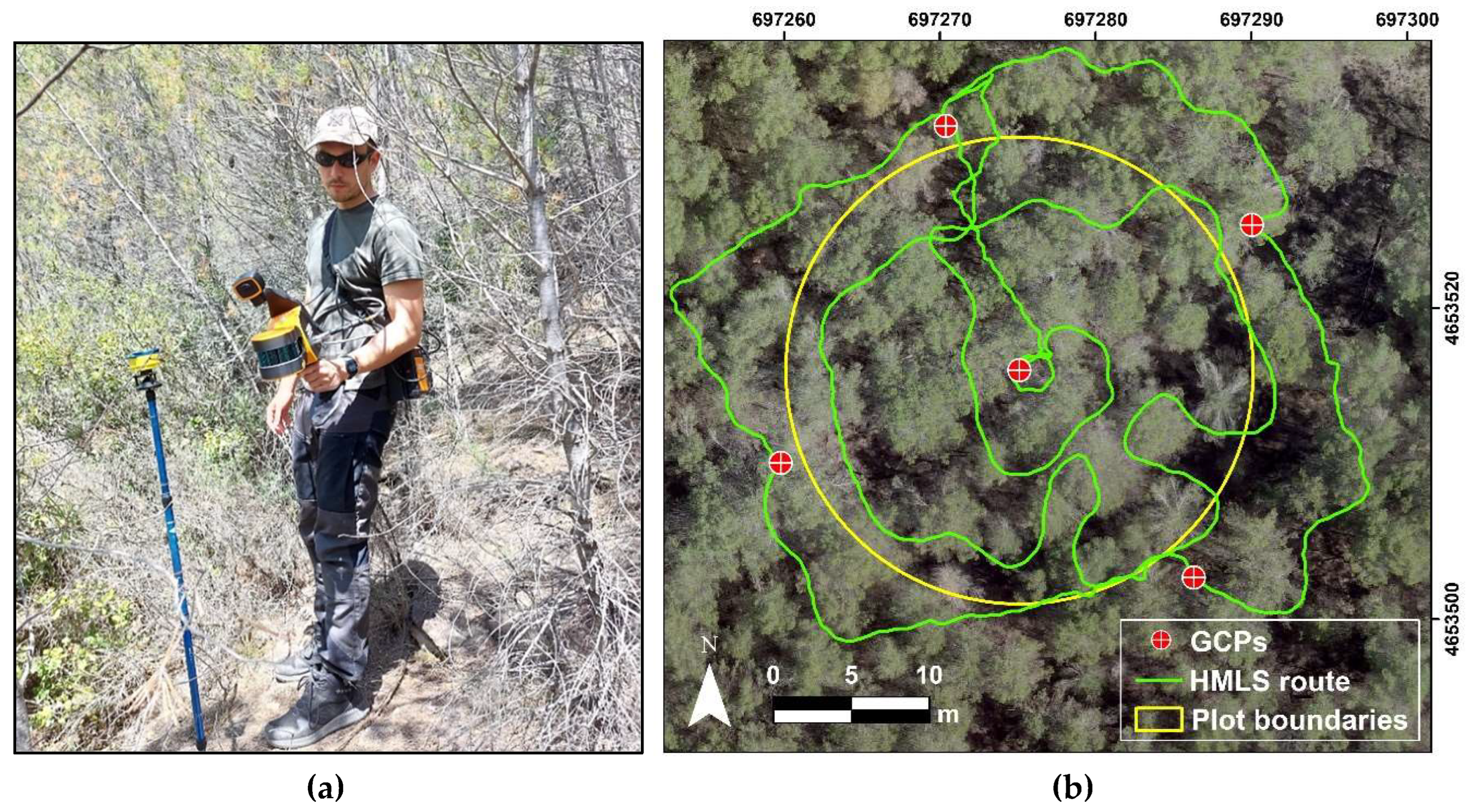
Figure 3.
Result of voxelization (below) of the point cloud (above) for the entire forest plot `al02´ (left) and for an individual tree within the plot (right). For a better visualization, only the filled voxels are displayed.
Figure 3.
Result of voxelization (below) of the point cloud (above) for the entire forest plot `al02´ (left) and for an individual tree within the plot (right). For a better visualization, only the filled voxels are displayed.
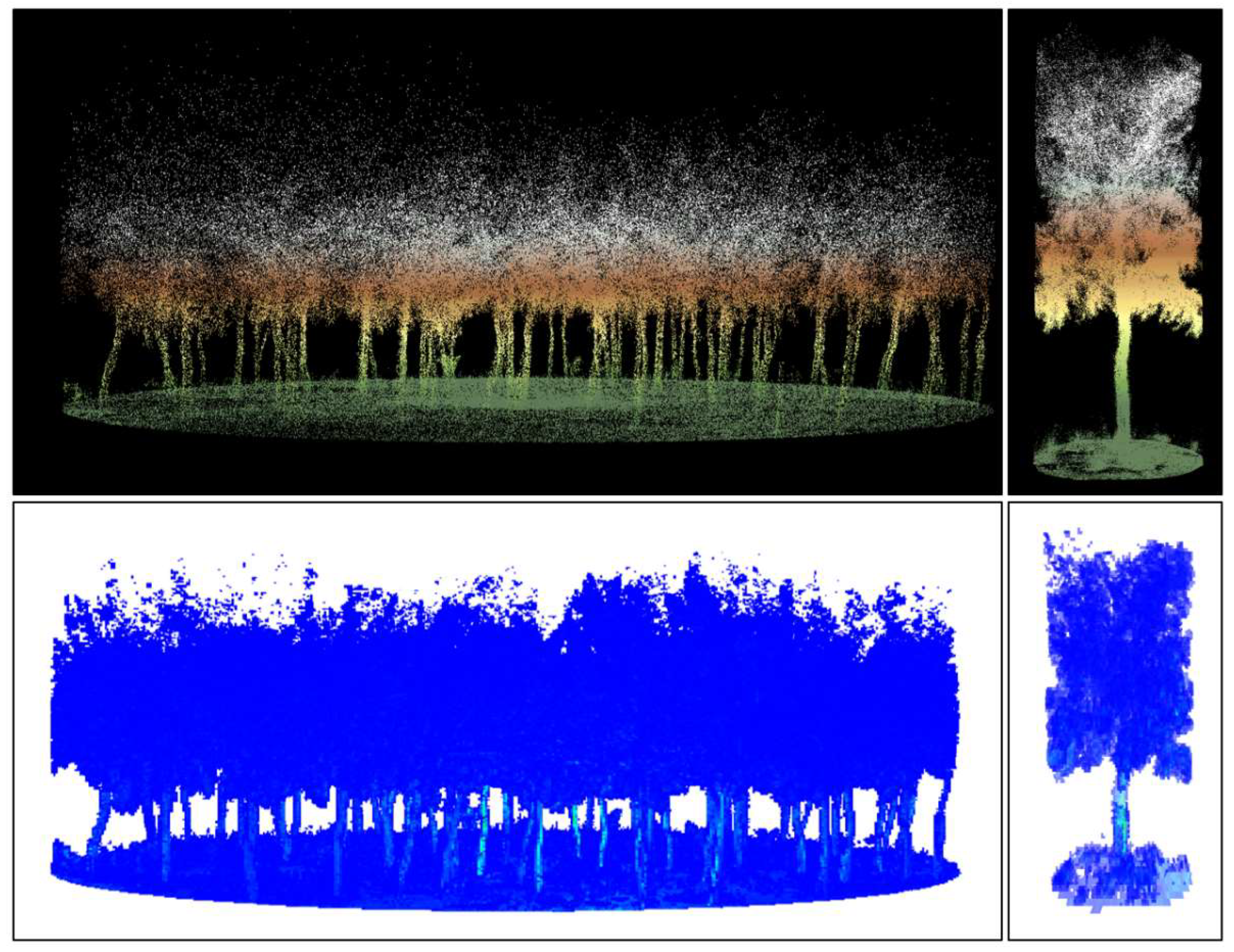
Figure 4.
Spatial distribution of the HMLS point cloud by representative plots (above) and transects (below) for each Prometheus fuel type considered in the study.
Figure 4.
Spatial distribution of the HMLS point cloud by representative plots (above) and transects (below) for each Prometheus fuel type considered in the study.
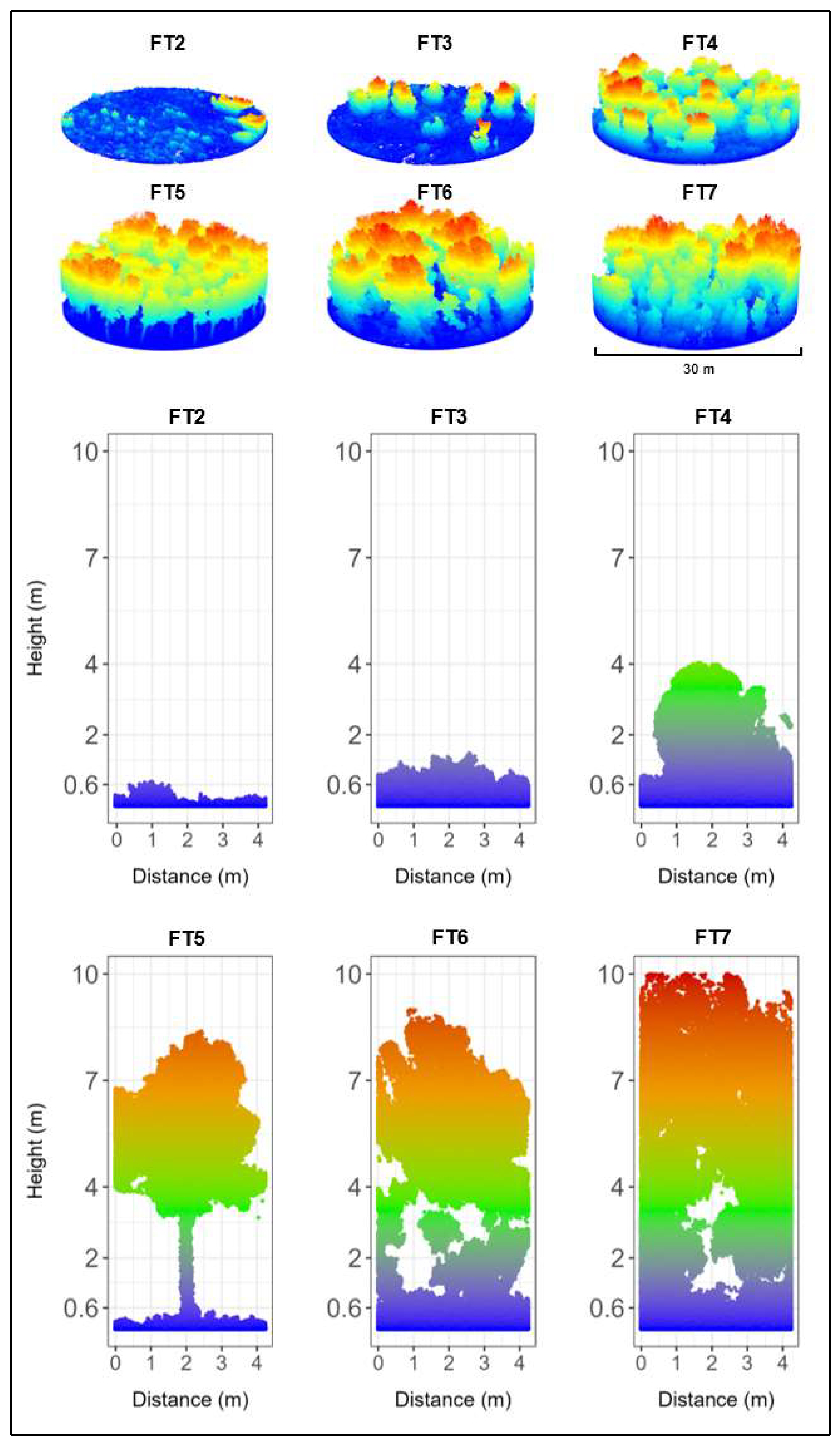
Figure 5.
DEMs mean height error for each forest plot and each pairs of ground point classification algorithms considered in the study.
Figure 5.
DEMs mean height error for each forest plot and each pairs of ground point classification algorithms considered in the study.
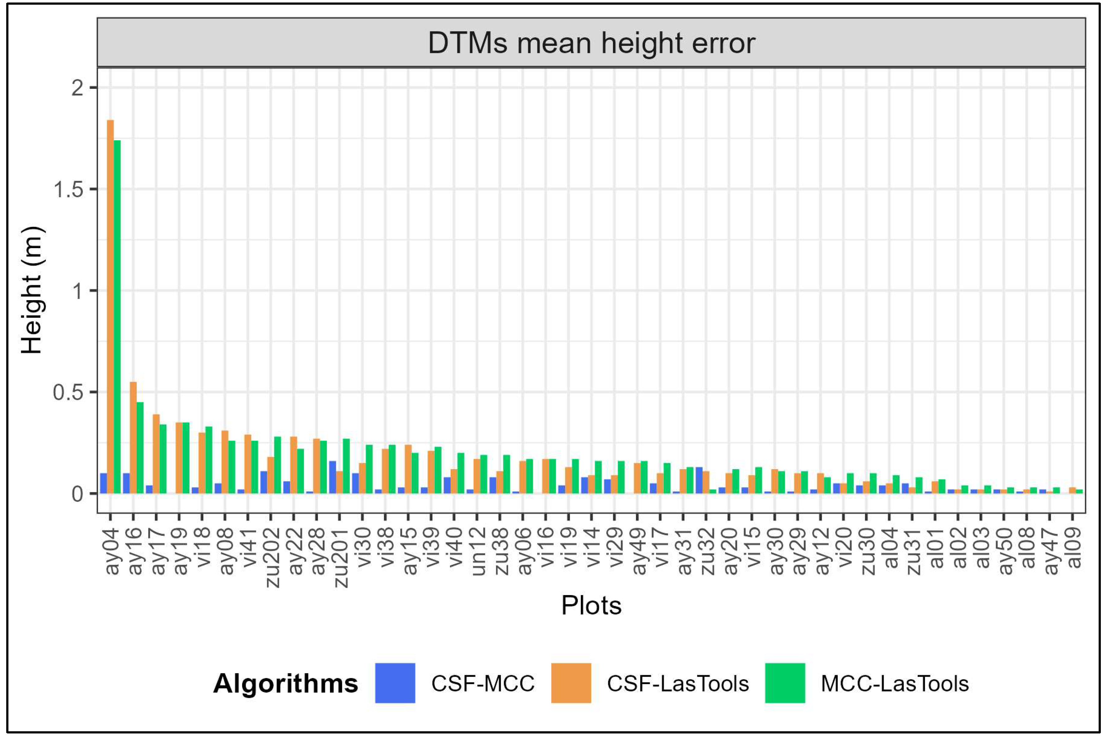
Figure 6.
Vertical distribution of the volume of fuel load every 0.05 m of the Prometheus shrub fuel types. Each line represents a forest plot arranged by the fuel type estimated in the field (left) and corrected with HMLS data (right). No modifications were made in FT4 plots.
Figure 6.
Vertical distribution of the volume of fuel load every 0.05 m of the Prometheus shrub fuel types. Each line represents a forest plot arranged by the fuel type estimated in the field (left) and corrected with HMLS data (right). No modifications were made in FT4 plots.
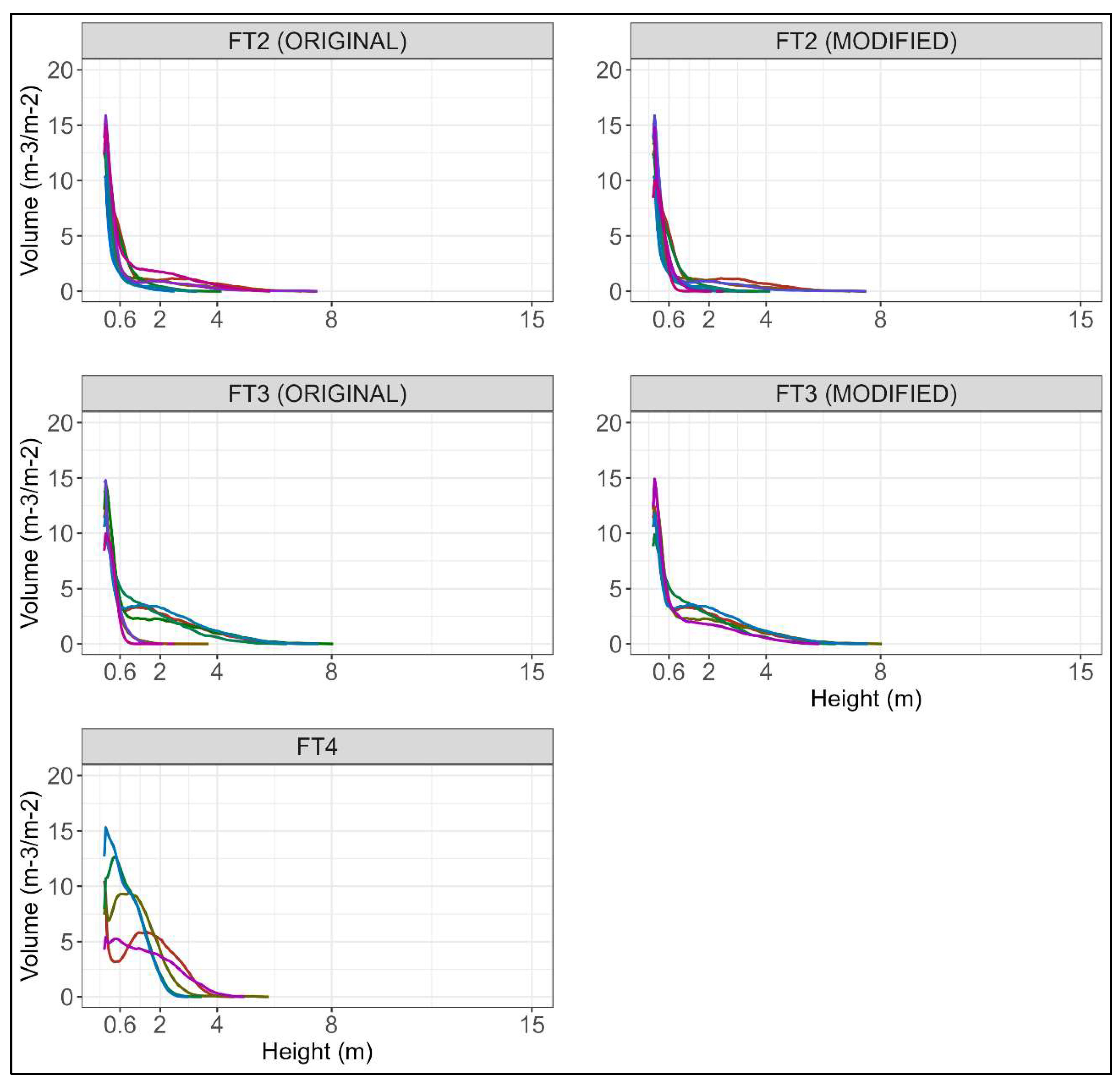
Figure 7.
Vertical distribution of the volume of fuel load every 0.05 m of the Prometheus tree fuel types. Each line represents a forest plot arranged by the fuel type estimated in the field (left) and corrected with HMLS data (right).
Figure 7.
Vertical distribution of the volume of fuel load every 0.05 m of the Prometheus tree fuel types. Each line represents a forest plot arranged by the fuel type estimated in the field (left) and corrected with HMLS data (right).
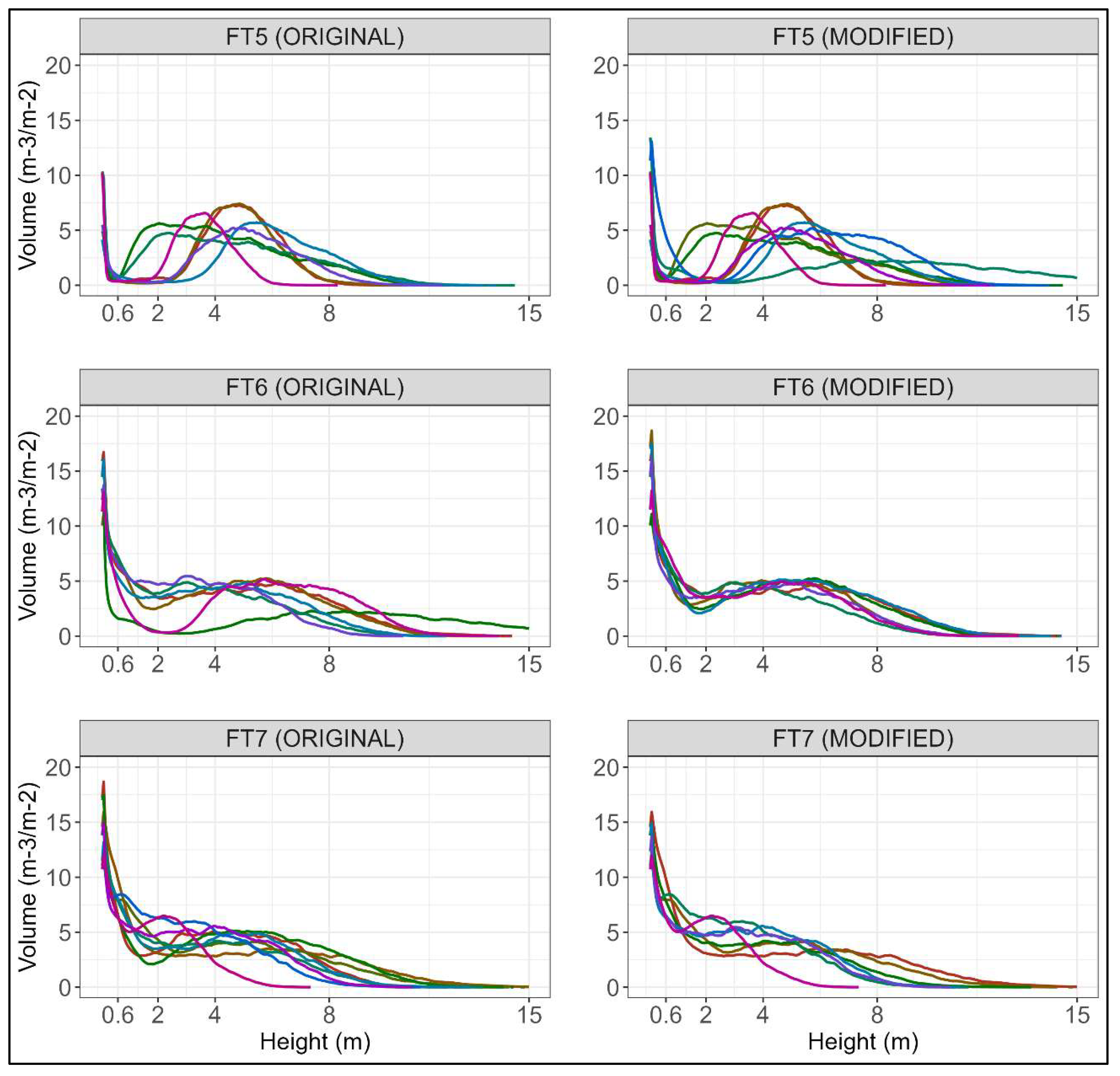
Figure 8.
Total volume (left) and percentage of the total volume (right) of fuel load for each plot by Prometheus height strata and for the Prometheus shrub fuel types. Percentage values within barplots are represented in %. Volume < 3% is not labeled due to space constraints. The plots are arranged by the fuel types modified from the HMLS data.
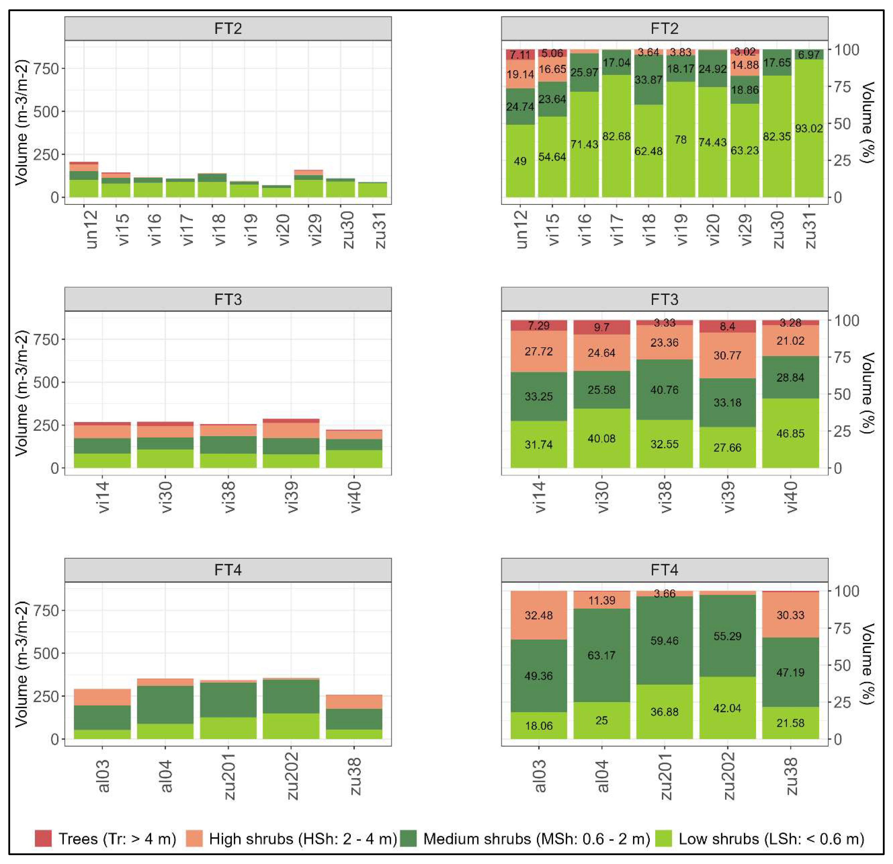
Figure 9.
Total volume (left) and percentage of the total volume (right) of fuel load for each plot by Prometheus height strata and for the Prometheus tree fuel types. Percentage values within barplots are represented in %. Volume < 3% is not labeled due to space constraints. The plots are arranged by the fuel types modified from the HMLS data.
Disclaimer/Publisher’s Note: The statements, opinions and data contained in all publications are solely those of the individual author(s) and contributor(s) and not of MDPI and/or the editor(s). MDPI and/or the editor(s) disclaim responsibility for any injury to people or property resulting from any ideas, methods, instructions or products referred to in the content. |
© 2023 by the authors. Licensee MDPI, Basel, Switzerland. This article is an open access article distributed under the terms and conditions of the Creative Commons Attribution (CC BY) license (http://creativecommons.org/licenses/by/4.0/).
Copyright: This open access article is published under a Creative Commons CC BY 4.0 license, which permit the free download, distribution, and reuse, provided that the author and preprint are cited in any reuse.


