Submitted:
26 December 2023
Posted:
27 December 2023
You are already at the latest version
Abstract
Deep learning heavily relies on statistical correlations to drive artificial intelligence (AI) innovations, particularly in computer vision applications like autonomous driving and robotics. However, despite providing a solid foundation for deep learning, these statistical correlations can be vulnerable to unforeseen and uncontrolled factors. The lack of prior knowledge guidance can result in spurious correlations, introducing confounding factors and affecting the model's robustness. To address this challenge, recent research efforts have focused on integrating causal theory into deep learning methodologies. By modelling the inherent and unbiased causal structure, causal theory can potentially mitigate the impact of spurious correlations effectively. Hence, this paper explores the basics of causal methodologies in image classification.
Keywords:
causal inference
; deep learning
; computer vision
; image classification
; statistical correlation
; causal learning
; domain generalization
; neural networks
; interpretability in AI
1. Introduction
The advent of artificial intelligence (AI) has ushered in transformative changes across diverse domains, demonstrating its vast potential in real-world applications [1,2,3,4,5,6,7,8,9,10,11]. Among its various facets, deep learning, a subset of AI, has made significant strides, particularly in the realm of computer vision. This progress is evident in its pivotal role in enhancing technologies like autonomous vehicles [12,13], drones [14,15], and robotics [16]. These advancements are supported by innovative training strategies, including attention mechanisms [17,18], pre-training techniques [19,20], and the development of generic models [21,22].
Simpson’s paradox [23] highlights this shortcoming. For instance, the connection between coffee consumption and neuroticism exhibits a positive association within each individual, yet individuals who consume more coffee generally display lower levels of neuroticism. While at the individual level, there is a positive correlation between coffee consumption and neuroticism, at the population level, this correlation takes on a negative aspect. This paradox is intriguing, highlighting the significance of multiple levels of interpretation yielding distinct outcomes from the same dataset. Consequently, both individual-level and population-level statistical correlations fall short of fully capturing the nuanced relationship between coffee consumption and neuroticism. In contrast, causal inference methods offer a solution by incorporating prior knowledge about causal structures. These methods discern accurate causal chains at specific levels of interpretation. As a result, causality-based approaches offer superior logical and effective outcomes compared to their statistical correlation-based counterparts [24]. This underpins the importance of scrutinizing.
In the real deep learning-based computer vision classification tasks, the typical objective revolves around effectively handling images denoted as X. The overarching aim is to train a neural network capable of accurately predicting the corresponding label Y [25]. To achieve this, a statistical model is employed, tailored with a well-suited objective function, which in turn helps estimate the conditional probability distribution . However, it’s important to note that this estimation holds true only when operating under the assumption of an independent identical distribution (I.I.D.). The I.I.D. hypothesis necessitates that the learned conditional probability distribution remains applicable not just within the confines of the training dataset, but also extends seamlessly to the testing dataset. This condition hinges on the expectation that novel prediction samples align with the distribution characteristics of the original training set.
Techniques like domain adaptation [26] and generalization [27] have emerged to bridge distribution gaps. Still, challenges persist, particularly with model interpretability [25]. Thus, while current methods prioritize function approximation, a more analytical approach could optimize generalizability and interpretability. Due to its inherent strengths, causality has garnered substantial attention in recent times, finding its foothold across various domains including statistics [28,29], economics [30,31], epidemiology [32,33], and computer science [34,35]. At its core, causal methodologies can be bifurcated into two primary facets: causal discovery and causal inference [36]. With the underpinnings established by causal discovery, causal inference capitalizes on these relationships for deeper analysis. In the ensuing sections, an example will elucidate the superiority of causality-focused approaches. This review delves deeply into the implications of causal theory as applied to vision and vision-language endeavours. These undertakings span a spectrum from classification and detection to segmentation, visual recognition, image captioning, and visual question answering. For every delineated task, we articulate a clear problem definition grounded in causal principles. Through a causal lens, we illuminate the intricacies involved in conceptualizing these tasks. After establishing the foundation, we thoroughly explore the current scholarly contributions in these areas. There are many studies on causal theory. For example, Kaddour et al. [37] grouped causal machine learning studies into five types and compared them. Gao et al. [38] looked at how causal reasoning can be used in recommendation systems. Li et al. [39] discussed the benefits of using causal theory in industries.
2. Preliminaries
2.1. Causation vs Correlation
The phrase “correlation is not causation” explains that just because two things seem to relate to each other, it doesn’t mean one is causing the other. When looking at lots of data that follow the same pattern, statistical learning can do a good job. But, if the data does not follow the same pattern, these methods often don’t do as well. For instance, in image recognition, a model might guess “bird” when it sees “sky” in the image just because birds and sky often show up together in the data. Causal learning [43] is different, aiming to find cause-and-effect links beyond just connections in the data. To learn about causality, machine learning needs to not only guess outcomes from repeated experiments but also think from a cause-and-effect viewpoint. Causal reasoning comes in three levels [44] (shown in Table 1). The first level is an association, like asking, "How might the weather change when the sky turns grey”. This just looks at how two things are linked. The second level is intervention, where you ask about what happens if you take a certain action, like “Will I get stronger if I work out every day?” You can’t answer this just by looking at links in the data. For example, if you only saw that a person who works out every day isn’t stronger than a professional athlete, you might wrongly think that working out doesn’t make you stronger. The third level is counterfactual, where you think about “what if” situations that didn’t actually happen. It tries to compare different results from the same situation, but the starting point of the “what if” question is not real.
Figure 2 shows statistical correlation-based techniques with causality-based methods, applying both to an identical image classification task. Given the input images of a dog alongside the corresponding labels, as seen in Figure 2(a), the model is trained for accurate identification. Figure 2(b) showcases the visualizations of the features discerned during the learning process. The intricacies of both the statistical correlation-based and causality-based learning methodologies are detailed in Figure 2(c). Owing to the frequent co-occurrence of the dog and the grassland within the training dataset, the statistical correlation-driven approach tends to misconstrue the grassland traits as pivotal for labelling, attributing this to their analogous distribution. Contrarily, causality-based techniques pivot more towards the inherent cause chain, prioritizing features intrinsic to the dog. These disparate learning frameworks culminate in varied classification outcomes, particularly evident when processing uncommon samples, as depicted in Figure 2(d). Confronted with an image of a dog set against a snowy backdrop, the statistical correlation-focused model stumbles, being unable to correctly label due to the absence of familiar grassland traits. In stark contrast, the causality-based model, honing in on the quintessential dog features, succeeds in accurately identifying the subject by leveraging causal attributes. Consequently, causality-centric methods anchor not merely on the homogeneity of data patterns but also on the inherent dynamics that carve out the causal relationships between variables [45]. This imparts them with resilience in unfamiliar terrains and augments the interpretability of their learning trajectory.
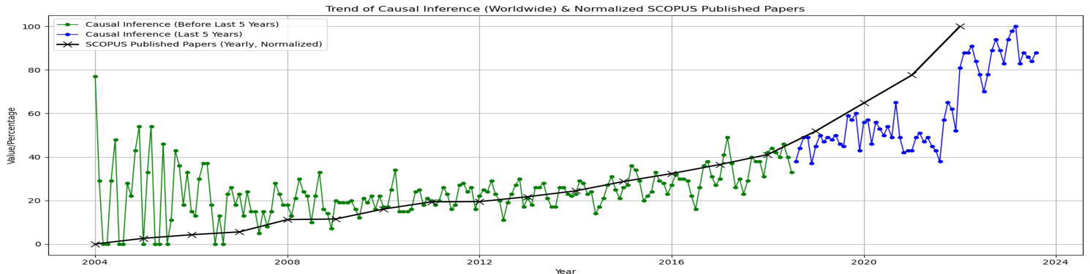
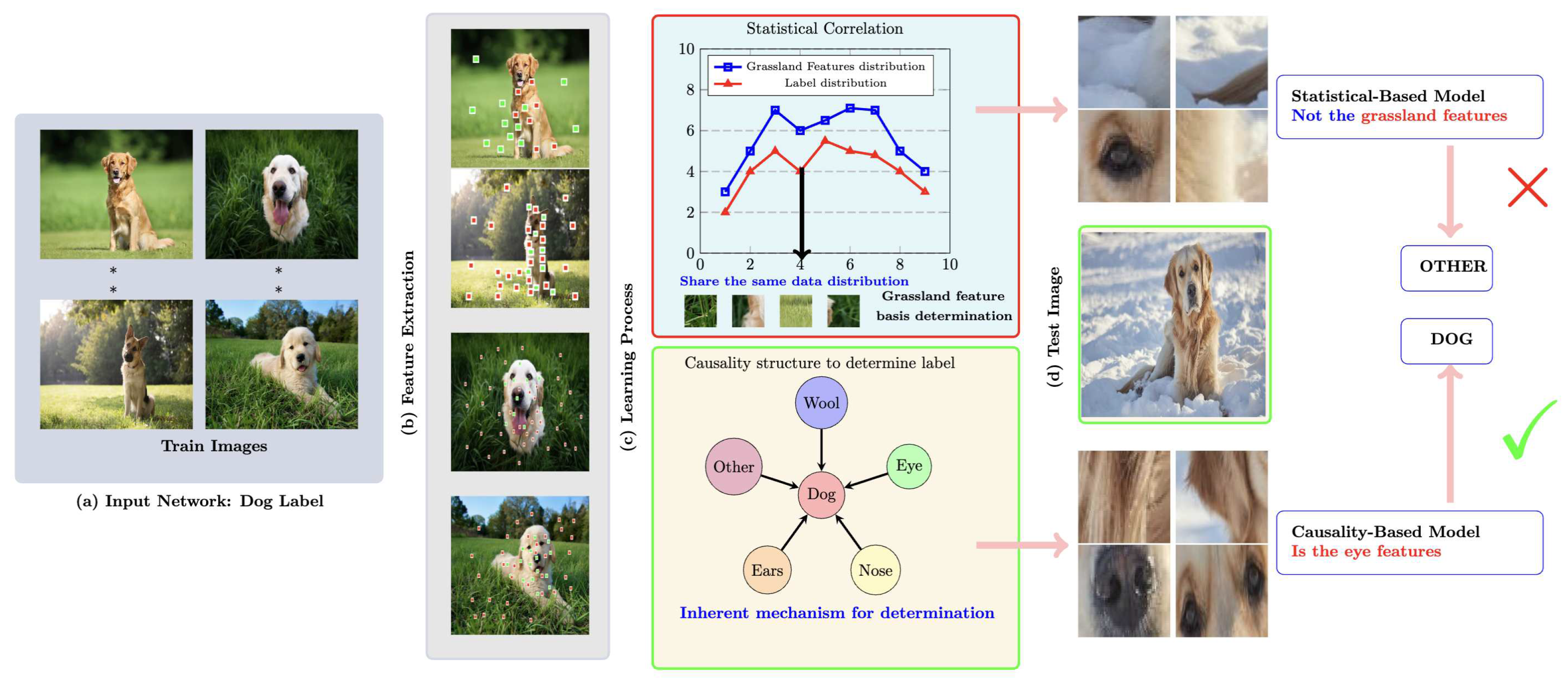
Figure 1.
This plot illustrates the dynamic evolution of interest in causal inference (blue line: Google search interest, black line: Scopus publications), spanning 2004 to 2023. A significant surge in the last five years reflects the expanding recognition of causal inference’s applicability across diverse domains. This trend underscores the pivotal role of causal inference in shaping contemporary scientific discourse and a deeper understanding of causal dynamics.
Figure 2.
Presented here are images and their respective labels processed by an image classification network for the purpose of feature extraction, following which analytical decisions are made regarding the features, and lastly, the respective labels are outputted. The illustration above juxtaposes two different learning mechanisms: statistical correlation-based analysis and causality-based analysis, as delineated in (c). The input in (a) is represented visually through feature extraction in (b). Green boxes indicate the isolated non-causal features, while the red boxes show the isolated causal features. Due to variations in learning mechanisms, the method grounded on statistical correlation is unable to derive the correct label. In stark contrast, the causality-based method can identify the correct label, as displayed in (d). When introduced to the learned object in an unfamiliar environment, the correlation-based method is prone to be skewed by data bias. On the other hand, the causality-based method zeroes in on only the causal factors linked with the object and remains undisturbed by data fluctuations. The object of focus, in this case, is a dog instead of a sheep to demonstrate these principles.
2.2. Causal Discovery
2.2.1. Causal Structure
A causal structure is characterized as a directed acyclic graph (DAG) wherein each node denotes a distinct variable, and every edge represents a direct functional relationship between the connected variables [43]. In this representation, if an edge is directed from Y to X, then X is termed the child variable and Y is the corresponding parent variable. A variable is deemed endogenous if it possesses a parent variable within the causal structure; if not, it is exogenous.
For a clearer understanding, let’s refer to the causal structure depicted in Figure 4 (I), which serves as a model for the process of image generation. In this structure, four nodes are present: X is the image in question, Y is its corresponding label, C stands for the content of the image, and D refers to its domain. The relationship emphasizes that an image is a representation of both its domain and content attributes. On a related note, the edge showcases the essence of a vision task: to aptly label the input image. Further, the edge indicates that the content within an image predominantly dictates its label. Given that X is influenced by two edges, and , it stands to reason that both D and C are parental entities to X. Notably, D is an exogenous variable since it doesn’t have any parent variables within this structure. The term path, in this context, signifies the series of edges connecting two variables. Therefore, in Figure 4 (I), the likely paths linking X and Y could be or .
In the context of the causal structure illustrated in Figure 4 (I), it’s imperative to address the concept of conditional dependence. Conditional dependence refers to the relationship between two variables when conditioned on a third variable. Observing the edges of the structure, one can infer potential conditional dependencies. For instance, the relationship between X and Y becomes apparent when considering the content C—if we know C, our belief about Y might change after observing X. This is due to the paths and , both indicating relationships that can potentially change based on the known variables. Furthermore, D and C might exhibit a form of conditional independence with Y if X is observed, since X acts as a collider on the path from D to Y through C. Analyzing such conditional dependences is pivotal as it offers insights into how altering one variable might affect others in the causal framework, particularly when certain conditions are met. To understand conditional dependencies in DAGs, d-separation a tool that identifies (conditional) relationships between variables. For large graphs, determining the (conditional) independence of two nodes is not immediately evident. The concept of d-separation provides an algorithmic mechanism for this verification, as proposed by [46]. To effectively leverage this tool, it is essential to comprehend the subsequent terminologies:
- A path from X to Y constitutes a sequence of nodes and edges with X and Y being the initial and terminal nodes, respectively.
- A conditioning set L refers to the collection of nodes upon which we impose conditions. It’s noteworthy that this set might be vacant.
- Imposing conditions on a non-collider present along a path invariably blocks that path.
- A collider on a path inherently obstructs that path. Nonetheless, conditioning on a collider, or any of its descendants, unblocks the path.
Given these elucidations, nodes X and Y are termed d-separated by L if conditioning on all elements in L obstructs every path interlinking the two nodes.
2.2.2. Structural Causal Model
The causal structure provides a blueprint, and to realize this blueprint, a structural causal model outlines how each variable is influenced by its parental variables through effect functions. Given a set of variables representing nodes in the causal structure, their interrelation with parental variables and effect functions is expressed by Eq. (1):
In Eq. (1), represents the parent variables of , symbolizes the unobserved background variables including noise, and defines the functional relationship.
A comprehensive understanding of causal models requires the exploration of joint distributions of all these variables. Such distributions are crucial for determining how changes in one variable can influence others. This is where Eq. (2) becomes pivotal:
Eq. (2) offers a compact representation of these joint distributions. Termed the product decomposition, it breaks down the complex relationships between variables into simpler, more interpretable conditional probabilities. With this decomposition, causal relationships within a dataset can be systematically represented both by the causal graph and the corresponding joint distribution.
Taking a more specific look using the relationships of variables depicted in Figure 4 (I), the variable X is deduced as an outcome of its parent variables and the associated effect functions, given by:
Here, f is the designated effect function and U stands for the background variable in this functional bond. The overarching aim of causal inference is to decode f and to measure the effects of hypothetical interventions or counterfactual scenarios.
2.3. Causal Inference
Causal inference is central for understanding the effects of actions or interventions on results, particularly in fields like image classification. The decisions we make in such a setting, like choosing a domain D or the context C for image generation, might substantially influence the ultimate classification performance denoted by the label Y. Consider the image X. The domain D could represent different environmental conditions under which an image is captured. For instance, might mean the image was taken during daylight, and might suggest nighttime. The outcome, Y, indicates the label or classification accuracy resultant from the chosen domain and context C. Given our causal structure, we can perform causal interventions and counterfactual evaluations. The intervention aims to modify the structure by specifying certain data and altering the relationship between the variables. Counterfactuals, on the other hand, strive to forecast outcomes in situations opposing the observed scenario. Moreover, there are two distinct intervention methods: back-door adjustment and front-door adjustment. Both offer structured approaches to understanding and assessing the effects of interventions. To quantify the effectiveness of our domain choice D on image classification, we use the average treatment effect (ATE). The counterfactual outcome, in this case, would elucidate the classification label Y in the counter scenario for the domain. Mathematically, the ATE for can be expressed as:
Where portrays the potential classification when domain D is fixed to d. If the image is captured during daylight (), then constitutes the counterfactual outcome of the predicted classification had the image been taken during nighttime. In practical scenarios, observing every possible outcome can be challenging. We might have data for images captured during the day but lack those taken at night, or vice versa. Gathering data for all scenarios can be resource-intensive or occasionally impractical. Hence, causal inference offers a toolkit for making informed decisions in the face of these challenges.
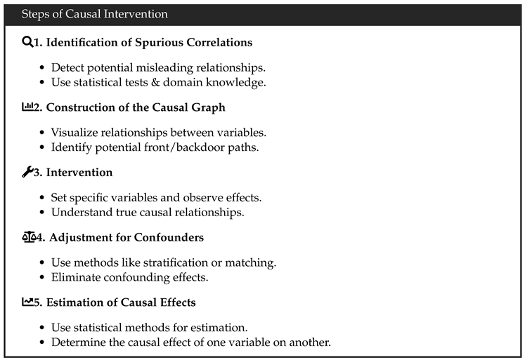
2.3.1. Causal Intervention
Causal interventions in machine learning provide a mechanism to actively manipulate one or more variables to assess the resultant changes in other variables. This deliberate manipulation often symbolized with the do-calculus notation , essentially blocks the influence of parent variables on X and assigns a new value x to it.
When looking to unearth the causal relationships in data, this intervention modifies the underlying graphical model, thus tweaking the associated conditional probabilities. This can be visually illustrated using Figure 4 (I). For instance, by performing a causal intervention on the domain variable, we can inspect its direct effects on labels, expressed as , while keeping other variables stable.
Nevertheless, due to the intricate interplay among variables, directly establishing the causal sequence between cause and effect without distractions from extraneous correlations can be difficult. Hence, interventions are crucial to maintaining independence among variables when pinpointing direct causal relationships. Taking reference from Rebane et al. [47], the fundamental interconnection architectures among three variables X, Y, and C are depicted in Figure 3.
Different structures necessitate varied intervention techniques due to their distinct properties. For instance:
- The path in Figure 3(a) represents a chain junction, with X impacting Y through an intermediary C. In the realm of visual tasks, features derived from an image inform the label. Here, intervening on C can obstruct the X to Y path.
- Figure 3(b) showcases a confounding junction, denoted by . Here, C influences both X and Y. Such contexts might introduce unintentional correlations in the true causal link between images and labels. Intervening on C can counteract this.
- The configuration in Figure 3(c) is termed a collider, where both X and Y dictate C. For vision tasks, the image might be shaped by both content and domain specifics. Here, if C remains unknown, X and Y are independent. Yet, knowing C ties X to Y, making intervention on C ineffective.
To ensure variable independence and mitigate confounder effects, causal interventions are necessary. The chosen approach depends on the structure, with two techniques explained below.
Back-Door Adjustment
stands as a pivotal technique in causal intervention for addressing confounding effects [43]. It is particularly concerned with paths that lead from X to Y, initiated with an arrow directed towards X Figure 3(d). Suppose we aim to determine the causal effect between. X and Y using Bayes’ rules. One might naturally compute:
However, this computation does not accurately capture the causal effect due to the presence of confounding paths. Given a scenario involving three variables, X, Y, and C, we visualize this configuration in Figure 3(d). Recognizing the path as the confounding junction structure, an effective strategy to block this path necessitates intervening on C, especially when C value is known [48]. A common intervention approach entails stratifying C and then computing the average causal effect for each segment. This adjusted configuration can be observed in Figure 3(e). Mathematically, the back-door adjustment can be expressed as:
Applying this adjustment facilitates the derivation of Y’s probability contingent upon X. Essentially, it reflects the causal relationship between the two, realized by summing over the conditional probabilities and the distributed probability associated with the confounder C.
Front-Door Adjustment
When we lack access to certain data, particularly for variable C, the back-door adjustment becomes ineffective. In such scenarios, we resort to the front-door adjustment. This strategy introduces a mediator, denoted by M, between X and Y. It serves as an intermediary in their causal relationship. The interaction is visually depicted in Fig. Figure 3(f).
Effect of X on M: To understand the influence of X on M, we ensure other interactions, particularly from Y, are negated. Formally, this relationship can be expressed as [43]:
Effect of M on Y: While measuring the impact of M on Y, we must account for any influence X might exert. This can be represented mathematically as [43]:
Combining the Two Interactions: To measure the overall interaction from X to Y via M, it can be expressed as:
The front-door technique helps in measuring the probability of Y conditioned on X by utilizing M as a mediator. When all necessary data is accessible, the back-door adjustment is apt. In contrast, if some data, such as C, is absent, the front-door adjustment becomes the preferred choice.
2.3.2. Counterfactual
Counterfactual reasoning is a method of causal inference that explores “what-if” scenarios. It contrasts observed data with hypothetical outcomes under different conditions [48]. In image processing, error terms highlight the deviation between actual and hypothetical outcomes [12]. For instance, by changing an attribute in an image, like a car’s colour from red to blue, and observing classification changes, one can assess the importance of that attribute. If a model recognizes the car in one colour but not the other, it may indicate an over-reliance on that particular attribute.
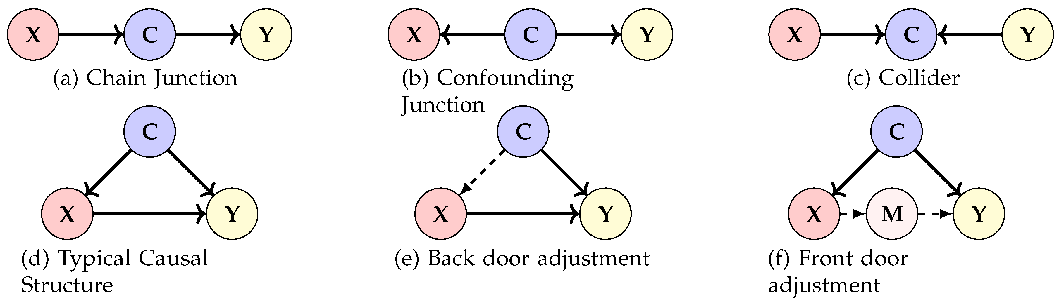
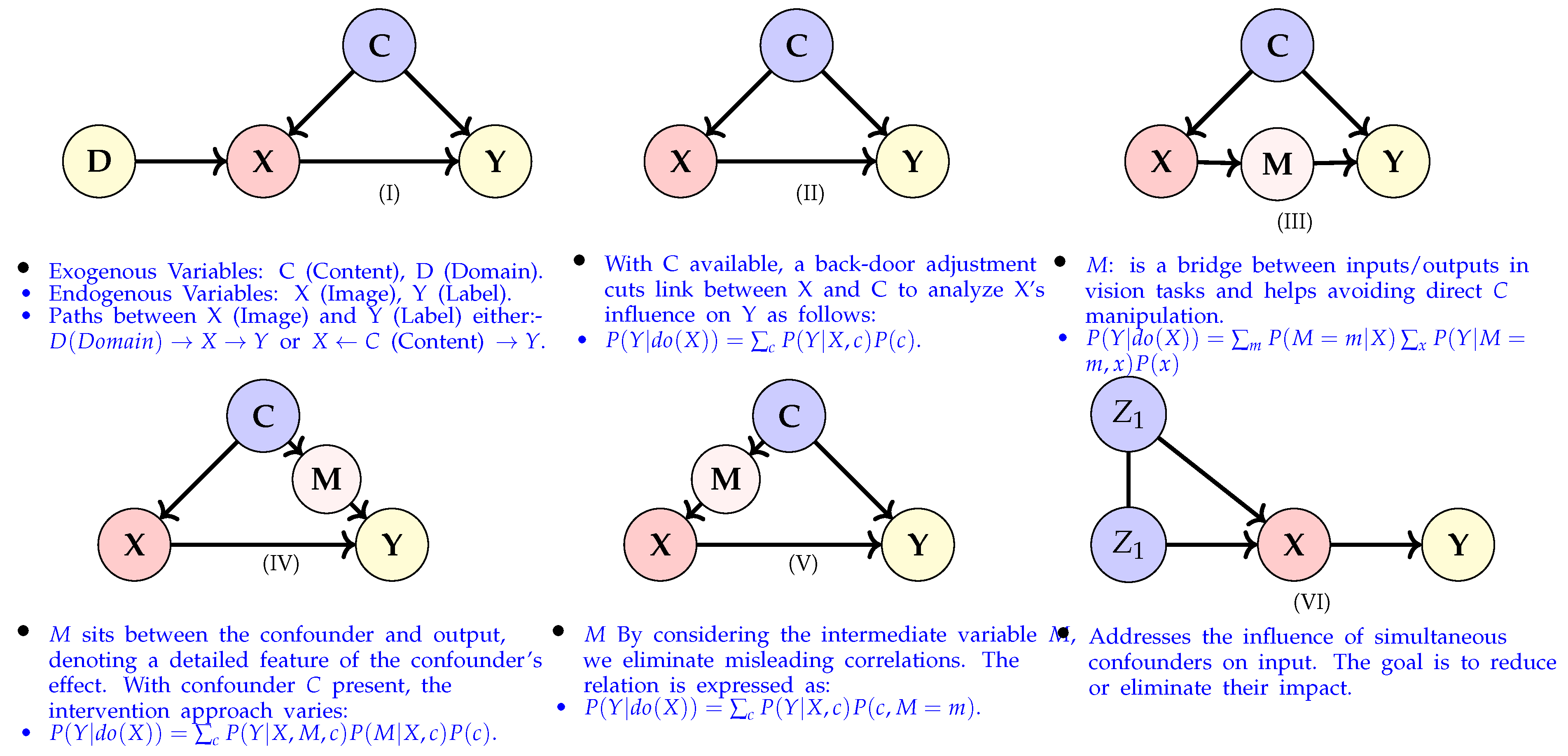
Figure 3.
Common Causal Graphs.
Figure 4.
Common structures.
3. Causality in Image Classification Tasks
Understanding causality is fundamental in various machine-learning tasks. By acknowledging the relationships between variables, we can build models that not only predict but also explain phenomena. In this section, we explore how causality intertwines with different tasks.
3.1. Classification
Causality has gained significant attention among researchers due to its ability to unveil true cause-and-effect relationships in real-world domains. This pivotal approach has found its way into various research avenues, including in the context of image classification. While remarkable achievements have been made, such as achieving State-of-the-Art (SOTA) accuracy on diverse datasets, a substantial challenge persists. Traditional models heavily rely on statistical correlation. They tend to learn from spurious correlations present in the training data, rendering them sensitive to deviations from the training distribution. Consequently, when faced with samples from distributions that differ significantly, these models falter in their classification endeavours. To surmount this critical limitation, researchers have turned their attention towards leveraging causal inference.

Table 2.
Causal Inference in Classification Tasks.
| Task | Paper | Year | Problem | Causal Instrument | Confounder | Base models | Structure |
|---|---|---|---|---|---|---|---|
| [49] | 2015 | Domain Adaptation | Causal Inference | Domain | - | I | |
| CLS | [50] | 2017 | Selection Bias | Causal Inference | Context | CRLR algorithm | I |
| [51] | 2020 | Understanding | Potential outcome model (DE) | Confounded concept | AutoEncoder | V | |
| [52] | 2020 | Imbalanced data | Back-door adjustment (TDE) | Optimizer | ResNeXt-50- | III | |
| [53] | 2021 | Catastrophic Forgetting | Potential outcome models (TDE) | old data | Transformer | I | |
| [54] | 2021 | OOD | Causal inference | Context | - | I | |
| [55] | 2021 | Generalization | Causal inference | Domain | Resnet50 | I | |
| [56] | 2021 | Generalization | Causal inference | - | Auto-Encoder | I | |
| [57] | 2021 | Domain Adaptation | Causal inference | Unobserved feature | CycleGAN | I | |
| [58] | 2022 | Domain Generalization | Causal inference | Causal factors | - | I | |
| [59] | 2022 | OOD | Causal inference | Unobserved latent variable | - | I | |
| [60] | 2022 | Domain Generalization | Potential outcome models | Domain | - | I | |
| [61] | 2023 | noisy datasets | Potential outcome models | Unobservable variable | - | I | |
| [62] | 2023 | catastrophic forgetting | Back-door adjustment | Task identifier | - | I | |
| [63] | 2023 | Domain Generalization | Counterfactual | Semantic concept | - | I |
3.1.1. Handling Long Tail Dataset
In recent years, computer vision advancements have been driven by datasets like ImageNet and MS-COCO [64,65]. Expanding these datasets to cover a wider class vocabulary exposes the challenge of long-tailed class distributions following Zipf’s law [66]. This imbalance becomes more pronounced when boosting data for data-poor tail classes inadvertently increases samples from data-rich head classes. Achieving a perfect balance becomes impractical, particularly in instances like instance segmentation [67]. Addressing long-tailed classification becomes crucial when training deep models at scale. Recent efforts [68,69,70] have mitigated the performance gap between class-balanced and long-tailed datasets. However, a comprehensive theoretical framework is missing. The paradoxical nature of the long tail, with an inherent bias towards data-rich head classes. To address the aforementioned issue, Tang et al. [52] introduced a causal framework to enhance long-tailed classification. Their causal graph uncovers the momentum in SGD optimizers as a confounder influencing both sample features and classification logits.
The Causal classifier [52] leverages causal inference techniques to preserve beneficial momentum effects while mitigating detrimental impacts in long-tailed learning settings. The “good” causal effect pertains to the favorable factor that stabilizes gradients and accelerates training, whereas the “bad” causal effect indicates the accumulated bias resulting in suboptimal performance in tail classes. To improve bias approximation, the causal classifier employs a multi-head strategy that evenly distributes model weight and data feature channels into K groups. Formally, the classifier calculates original logits as follows:
where denotes the temperature factor and is a hyper-parameter. When , this classifier effectively transforms into the cosine classifier. During inference, the causal classifier eliminates the detrimental causal effect by subtracting the prediction when the input is null:
Here, represents the unit vector of exponential moving average features, and serves as a trade-off parameter controlling direct and indirect effects.
3.1.2. Domain Generalization
Imagine an image classifier that is learned from photos. Would it recognize sketches too? could a health classifier based on one person’s heart data work for someone else? These questions relate to a problem: when a machine learning tool is trained on one type of data, it might struggle with different situations [27]. It is like preparing for a sunny day but facing a rainy one. This is important, especially in deep learning, where even small changes in data can confuse models. Solving this issue is key to making models better at handling various situations.
3.1.3. Problem Definition
Let X be the input (feature) space and Y the target (label) space. A domain is defined as a joint distribution on . For a specific domain , we refer to as the marginal distribution on X, as the posterior distribution of Y given X, and as the class-conditional distribution of X given Y.
In the context of Domain Generalization (DG), we have access to K similar but distinct source domains , each associated with a joint distribution . Note that for and . The goal of DG is to learn a predictive model using only source domain data such that the prediction error on an unseen target domain is minimized. The corresponding joint distribution of the target domain T is denoted by . Also, for all .
Two fundamental types of DG scenarios are identified:
- Single-Source DG: In this case, training data stems from a homogeneous source domain, i.e., .
- Multi-Source DG: This setting involves the study of DG across multiple sources. The majority of research is focused on the multi-source DG scenario, where diverse and relevant domains () are available.
Lv et al. [58] presented a structural causal model that integrates both causal and non-causal factors, raw inputs, and category labels, as depicted in Figure 4 (II). This work addresses the limitations of statistical approaches in domain generalization by adopting a causal perspective. The authors introduce the Causality Inspired Representation Learning (CIRL) algorithm, which leverages a structural causal model to enforce representations that adhere to essential causal properties and simulate causal factors. The proposed representation learning approach comprises three key modules: the causal intervention module, the causal factorization module, and the adversarial mask module.
- Causal Intervention Module: This module focuses on separating causal factors from non-causal factors through do-interventions. By doing so, the causal factors remain unchanged despite non-causal perturbations. This process generates representations that are independent of non-causal influences.
- Causal Factorization Module: This module promote independence among representation dimensions. It achieves this by minimizing correlations between dimensions. This transformation converts initially interdependent and noisy representations into independent ones, aligning with the characteristics of ideal causal factors.
- Adversarial Mask Module: In this module, the representations efficacy for the classification task is enhanced. An adversarial masker identifies dimensions of varying importance. This step helps distinguish superior dimensions from inferior ones, allowing the former to contribute more significantly. As a result, the representations become more causally informative.
The optimization objective of the proposed Causality Inspired Representation Learning (CIRL) encompasses combining classification losses for both superior and inferior dimensions ( and ) with the causal factorization loss (). This optimization process is balanced by a trade-off parameter ().
With the same structure, a causal regularizer is proposed by Shen et al. [50] with the primary objective was to address the non-i.i.d. problem, characterized by distribution disparities between training and testing image sets that often lead to classification challenges. To mitigate this issue, they harness causal inference to scrutinize the causal influence of individual image features on corresponding labels, with the aim of identifying pivotal causal factors. By considering each image feature as an individual variable, they distinguish between treated and control images, thus enabling the estimation of causal effects. This unique methodology uncovers compelling causal impacts that endure across various distributions. This attemt is formally posed as the Causal Classification Problem, entailing the discovery of causal contributions for image features and the construction of an image classifier grounded in these contributions. The authors proposed algorithm synergistically combines a causal regularizer inspired by the concept of confounder balancing.
In the context of observational studies, the rectification of bias stemming from non-random treatment assignments necessitates balancing confounder distributions. However, the authors depart from direct confounder distribution balancing and introduce a novel approach focused on equilibrating confounder moments by adjusting sample weights. The determination of these weights, represented as W, is accomplished through the optimization problem:
Here, and denote the mean values of confounders in treated and control samples, respectively, in the context of a specific treatment feature T. Notably, this method concentrates on the first-order moment, but it can be easily extended to incorporate higher-order moments. The authors intend to adapt this technique to simultaneously balance confounder distributions related to all treatment features.
Expanding upon the concept of confounder balancing, the authors introduce a causal regularizer:
In this equation, W signifies sample weights, and the term characterizes the loss associated with confounder balancing when considering image feature j as a treatment variable. encompasses all other features (treated as confounders) obtained from X by zeroing its jth column. denotes the jth column of the identity matrix I, and signifies the treatment status of unit i with regard to feature j. The underlying concept of this regularizer is its facilitation of estimating causal effects related to the treatment variable.
[53] The author’s objective revolves around comprehensively explaining the phenomena of forgetting and anti-forgetting within the framework of Class-Incremental Learning (CIL) through the lens of causal inference. This endeavour is undertaken by framing the data, features, and labels within causal graphs for each incremental learning step, effectively elucidating the underlying causal relationships governing these components. By adopting this approach, the author systematically dissects the mechanisms driving both forgetting and anti-forgetting in CIL.
Beginning with the causal graph, the author delineates the intricate relationships between old data (D), new training samples (I), extracted features (X and Xo), and predicted labels (Y and Yo). These relationships are represented by distinct links: I → X, X → Y, (D, I) → Xo, (D, Xo) → Yo, D → I, Xo → X, and Yo → Y as shown in (Figure 5).
Building upon the causal graph, the author proceeds to formulate the causal effect between variables through causal intervention, denoted as the do(·) operation. This operation effectively enforces specific values upon variables, resembling a “surgical” intervention within the graph. The objective is to isolate variables from their causal influences. With this framework in place, the author delves into explaining the rationale behind forgetting within the new training process. The causal effect of old data (EffectD) on new predictions is quantified, effectively capturing the causal essence of the previous knowledge. Notably, the author defines EffectD as the difference in predicted labels with and without the presence of old data, shedding light on the pivotal role of this metric in understanding forgetting.
To contrast forgetting, the author introduces the concept of anti-forgetting and dissects the causal effects that underpin this phenomenon. This exploration encompasses prevailing anti-forgetting techniques, including data replay, feature distillation, and label distillation. By leveraging the causal relationships depicted in the causal graph, the author meticulously analyzes the effects of these techniques in mitigating forgetting. The causal relationships enable an in-depth examination of the interactions between these techniques and the system dynamics. Specifically, the impact of data replay on causal relationships, the effects of feature and label distillation, and the introduction of non-zero effects are all cogently discussed in the context of thwarting forgetting.
Mahajan et al. [55] tackle the challenge of achieving effective generalization across domains in machine learning models. Their focus is on ensuring models can generalize accurately to new domains despite domain shifts.
The authors employ causal inference to understand relationships between variables. They create a Structural Causal Model (SCM) to depict data generation and variable interconnections in domain generalization. This causal approach helps them identify crucial causal features for cross-domain classification, leading to robust generalization.
The key steps of their approach are as follows:
- Recognizing the Confounder and Invariance Condition: The authors introduce the object variable O as a confounder that influences features X and class labels Y. They aim to find invariant representations across domains that are informative about O.
- Introducing the Matching Function : They propose a matching function to assess if pairs of inputs from different domains correspond to the same object. This function enforces consistency of representation across different domains but with the same object.
- Defining the Invariance Condition: An average pairwise distance condition between representations of the same object from different domains is stipulated. This condition ensures close representations for the same object across various domains.
- Learning Invariant Representations: To learn invariant representations, the authors introduce the “perfect-match” invariant, combining classification loss and the invariance condition. This loss function encourages representations that are invariant to domain shifts while preserving object-related information.
Liu et al. [54] address the challenge of out-of-distribution (OOD) generalization by mitigating the confounding effects of mixed semantic and variation factors in learned representations. The authors introduce a Causal Semantic Generative (CSG) model that explicitly models separate causal relationships between semantic and variation factors, enhancing the model’s performance on OOD examples. The key components of their approach include:
- Introducing the CSG model to represent causal relationships between semantic (s), variation (v), and observed data (x, y).
- Disentangling semantic and variation factors using latent variables s and v, ensuring accurate modeling of causal relations.
- Addressing confounding by attributing x-y relationships to latent factor z and accounting for interrelation between semantic and variation factors.
Sun et al. [56] tackled the challenge of degraded prediction accuracy due to distributional shifts and spurious correlation. They introduced a Latent Causal Invariance Model (LaCIM) to handle this confounding. LaCIM incorporates causal structure and a domain variable to address confounding issues. The authors identified a spurious correlation between latent factors S and Z, arising from an unobserved confounder C. This correlation can negatively impact model performance across domains. To address this, LaCIM employs a structural causal model framework, representing relationships between latent factors. A domain variable accounts for distributional shifts, while Disentangled Causal Mechanisms (DCMs) capture attribute-specific shifts. By leveraging DCMs, LaCIM replaces unobserved attributes with proxy variables, aiding model adaptation. The authors achieve this by implementing the transportability theory.
The paper by [57] et al. addresses the challenge of adapting models from a source to a target domain in the context of Unsupervised Domain Adaptation (UDA). UDA seeks to enhance model performance on a target domain without target domain labels. The authors introduce a novel approach called Transporting Causal Mechanisms (TCM) to bridge the domain gap. The authors identify a confounding factor, the domain selection variable S, as the key challenge in UDA. They propose using disentangled causal mechanisms as proxies for unobserved domain-specific attributes. The TCM approach involves three main steps: (1) identifying disentangled causal mechanisms that correspond to attribute-specific shifts, (2) using transformed outputs as proxy variables for unobserved attributes, and (3) transporting these mechanisms to align feature representations between domains. By substituting unobserved attributes with proxy variables derived from disentangled mechanisms, the authors effectively mitigate the confounding effect. The core intervention equation captures domain-specific shifts in a principled manner.
In their work [71], the authors introduce the Contrastive Causal Model (CCM) as a solution to the domain generalization problem. CCM employs contrastive similarity to convert new images into prior knowledge and amplify the causal effects from images to labels. The CCM framework comprises crucial components, including a teacher-student backbone, a classifier, and a knowledge queue. The approach encompasses domain-conditioned supervised learning, causal effect learning, and contrastive similarity learning. The authors identify a significant confounder in the domain generalization challenge, manifested as the spurious correlation introduced by domain shifts. This confounding factor can undermine genuine causal relationships among variables. To mitigate this confounding effect, the authors introduce a structural causal model (SCM) that explicitly delineates the causal paths from images to labels. This strategy serves to disentangle the authentic causal effects from the spurious correlations, thereby allowing the model to concentrate on the true causal relationships. The training of CCM encompasses a sequence of essential steps:
- Domain-Conditioned Supervised Learning: The model optimizes cross-entropy loss while conditioning on the domain. This strategy captures the correlation between images and labels across diverse domains.
- Causal Effect Learning: Leveraging the front-door criterion, the authors measure and enhance causal effects. A knowledge queue is leveraged to retain historical features and labels, aiding the translation of new images into acquired knowledge.
- Contrastive Similarity Learning: The application of contrastive similarity serves to cluster features sharing the same category. This process quantifies feature similarity, facilitating the separation of features.
Wang et al. [59] authors address the challenge of domain generalization building a classifier that performs well in unseen environments. The fluctuating correlation between features and labels across different environments hinders effective generalization. To tackle this, they propose a two-phased approach. First, a Variational Autoencoder (VAE) learns the data distribution for each environment, capturing latent variables responsible for inter-environment variations. Then, balanced mini-batch sampling is introduced. It pairs examples with similar balancing scores from VAE’s conditional prior, forming balanced mini-batches. This counters unstable correlations between features and labels across environments. The main confounder addressed is the variable correlation between label Y and latent Z across environments. This variance affects the causal relationship between features and labels, challenging robust generalization. A Variational Autoencoder (VAE) is employed to learn data distribution within each environment. Model parameters and latent variable Z are learned from training data. The model captures causal connections among Y, Z, and observed feature X. To manage varying Y-Z correlations across environments, the authors propose balanced mini-batch sampling. Dissimilar examples with matching balancing scores are paired, forming balanced mini-batches. This cultivates a balanced distribution that emphasizes stable Y-X causal relations. It mitigates adverse effects of unstable correlations in training data.
Wang et al. [60] addresses domain generalization by leveraging invariance in causal mechanisms to enhance model generalization across distributions while preserving semantic relevance for downstream tasks. The authors defined domains as distributions over input (X) and label (Y) spaces. They proposed aggregating instances from diverse domains into the training dataset D and employing Empirical Risk Minimization (ERM) loss to optimize encoding () and decoding () models. The paper connects neural networks and causal models, treating datasets as Structural Causal Models (SCMs). This interpretation enhances confidence in the neural model’s ability to capture causal mechanisms from observational data. The average Causal Effect (ACE) quantifies the influence of each input feature on the output. Neural network () serves as a tool for causal quantification, with a clear procedure for ACE computation. Inspired by contrastive representation learning, they introduced contrastive ACE loss. It identifies differences in ACE values across domains, optimizing interclass dissimilarity and intra-class similarity via positive and negative sets. Their training involves encoding and decoding model initialization, positive and negative set construction, and loss optimization using gradient descent. The innovative contrastive ACE loss, coupled with ERM, stabilizes performance against domain shifts.
The core problem addressed by Chen et al. [63] was the challenge of domain generalization, where a model trained on a single source domain must be capable of handling various unseen target domains. This scenario is characterized by the need to account for the domain shift between the source and target domains. The proposed solution introduced the novel “simulate-analyze-reduce” paradigm, which represents a comprehensive approach to mitigate the challenges posed by domain shifts in single-domain generalization. This paradigm comprises three primary stages: domain shift simulation, causal analysis, and domain shift reduction. The underlying idea was to first simulate domain shifts by generating an auxiliary domain through the transformation of source data. These shifts are based on variant factors, representing extrinsic attributes causing domain shifts. Subsequently, a meta-causal learning method was introduced, enabling the model to infer causal relationships between domain shifts in the auxiliary and source domains during the training phase. This inferred meta-knowledge is then utilized for analyzing the domain shifts between target and source domains during testing.
3.2. Practical: Problem Formulation
In computer vision, we often try to match images with the right labels, a task known as classification. Most current methods, like those in references [72,73], look at patterns between image features and labels. However, these methods can be thrown off by random patterns [61] or when data isn’t consistent [60]. That’s why it’s crucial to use causal theory, which helps understand the direct cause-and-effect between images and labels. As discussed earlier, the background of an image can create spurious correlations that affect prediction labels [74]. This problem can be explained using casual-and-affect as follows:
To systematically study how the background affects image label predictions, we can construct a causal graph [75,76] as shown in Figure 6, which has four variables: feature (X), background feature(C), model (M), and prediction (Y).
The causal graph represents a directed acyclic graph illustrating the interactions among the variables of interest, namely {C, X, M, Y}, through causal links. Each variable in the graph corresponds to a specific component of the image classification process: C represents the background features, which have the potential to influence both the input features X and the behaviour of the image classification model M. X denotes the input features utilized for image classification, encapsulating relevant information from the images. M stands for the image classification model itself, transforming input features X into predictions Y. Y represents the output predictions generated by the image classification model M.
Once we construct DAG to investigate, the cause-and-effect primary objective will, based on the causal graph in Figure 6, is to investigate the direct causal effect along the path . In the domain of causal inference, this effect is referred to as the Total Direct Effect (TDE) [76,77]:
Where Y symbolizes the prediction for the positive class, represents the set of all classes (in this instance, ), x corresponds to a specific input value, Y=1 positive class from {1,0} because we are interesting background effect on the positive class classification and denotes a different input value. The TDE quantifies the discrepancy in anticipated probabilities for the positive class when transitioning the input from to x while keeping other variables constant. This calculation reveals the direct impact of modifying input features on model predictions for the positive class in binary classification.
Before computing the final TDE, it is imperative to undertake de-confounded training. This process involves estimating ’modified’ causal graph parameters, removing any influence of undesirable ’background features’ while preserving the impact of crucial ’main features.’ During training, the do-operator neutralizes the confounding bias of ’background features’ and it ensures the learned model primarily relies on ’main features.’ Subsequently, during inference, the equation encapsulates a comparison between prediction probabilities when input is x and . This contrast captures the direct impact of changes in input features on model predictions.
By employing this approach, we gain insight into the extent to which changes in input features lead to variations in model predictions for the positive class, mitigating unwanted influence from confounding variables. This framework empowers us to discern the genuine impact of ’good’ features on model decisions and facilitates a more accurate understanding of the relationship between input features and predictions.
3.2.1. De-Confounded Training
To address the confounding effect introduced by the background variable C and isolate the direct causal effect of X on Y, we need to adopt a de-confounded training approach [52]. This approach aims to adjust the training process to focus on the direct causal relationship while mitigating the influence of the confounder C.
The foundation of our de-confounded training lies in the back-door adjustment principle [78]. Given the causal graph structure, in this case, we can modify the standard loss function to incorporate adjustments that account for confounding introduced by C. The adjusted loss encourages the model to emphasize the direct causal relationship between X and Y while reducing the impact of C. Mathematically, we can define our de-confounded training objective as the same as Eq. (13).
Our de-confounded training approach involves incorporating an attention penalty loss to estimate the Total Direct Effect () more accurately, especially in the presence of confounding introduced by the background variable C.
There are many ways to reduce the impact of background features on prediction, but the most widely used technique recently is attention-based. To achieve this, we can utilize an attention penalty loss in our training process. The attention penalty loss works in conjunction with the standard classification loss, such as nn.BCEWithLogitsLoss (as we are doing binary classification), which computes the loss between model outputs and ground truth labels. Additionally, the attention penalty loss takes into account an attention mask.
Mathematically, the combined loss is formulated as follows:
where the classification loss is calculated using the classification criterion, and the attention loss is determined by the mean of the attention mask:
where N is the number of samples in the batch, and is the attention mask calculated by the model for the ith sample.
By integrating this attention penalty loss into a de-confounded training approach, we can enhance the accuracy of estimating the Total Direct Effect. This augmentation is particularly crucial when addressing confounding variables introduced by the background variable C, thereby enabling a more precise evaluation of the direct causal effect of X on Y in the context of binary image classification.
4. Conclusion
This review explores how causal theory can be integrated into computer vision, transforming AI methodologies, particularly in image classification. Traditional machine learning models that rely on statistical correlations can struggle when faced with data distributions that differ from their training sets. In contrast, causal methodologies offer a more robust and interpretable approach by understanding the underlying cause-and-effect relationships. This is especially important in tasks such as domain generalization, handling long-tailed datasets, and combating issues like model forgetting. Key to advancing causal approaches in computer vision are structured causal models (SCMs), which provide a blueprint for understanding the complex relationships between different variables in image processing. Through causal inference and intervention techniques, SCMs enable the isolation of direct causal effects, offering a nuanced understanding of the interactions within the data. This is particularly important in scenarios involving domain shifts or dealing with out-of-distribution (OOD) generalization challenges. Looking to the future, the potential of causal inference in computer vision is immense. As we move towards more complex and dynamic real-world applications, the need for models that can not only predict but also explain their predictions becomes increasingly crucial. The integration of causal theory in computer vision paves the way for the development of AI systems that are not only more accurate and reliable but also more interpretable and adaptable to ever-changing data landscapes.h This is paper emphasizes the importance of transitioning from a mere correlation-based understanding to a causation-focused approach in computer vision. By doing so, we can significantly enhance the capability of AI systems to handle real-world variability and complexity, ensuring more reliable and effective applications in diverse domains such as autonomous driving, robotics, and beyond.
References
- Tamsekar, P.; Deshmukh, N.; Bhalchandra, P.; Kulkarni, G.; Hambarde, K.; Husen, S. Comparative analysis of supervised machine learning algorithms for GIS-based crop selection prediction model. Computing and Network Sustainability: Proceedings of IRSCNS 2018. Springer, 2019, pp. 309–314. [CrossRef]
- Kulkarni, G.; Nilesh, D.; Parag, B.; Wasnik, P.; Hambarde, K.; Tamsekar, P.; Kamble, V.; Bahuguna, V. Effective use of GIS based spatial pattern technology for urban greenery space planning: a case study for Ganesh Nagar area of Nanded city. Proceedings of 2nd International Conference on Intelligent Computing and Applications: ICICA 2015. Springer, 2017, pp. 123–132. [CrossRef]
- Hambarde, K.A.; Proenca, H. Information Retrieval: Recent Advances and Beyond. arXiv preprint arXiv:2301.08801 2023. [CrossRef]
- Hambarde, K.; Silahtaroğlu, G.; Khamitkar, S.; Bhalchandra, P.; Shaikh, H.; Kulkarni, G.; Tamsekar, P.; Samale, P. Data analytics implemented over E-commerce data to evaluate performance of supervised learning approaches in relation to customer behavior. Soft Computing for Problem Solving: SocProS 2018, Volume 1. Springer, 2020, pp. 285–293. [CrossRef]
- Husen, S.; Khamitkar, S.; Bhalchandra, P.; Tamsekar, P.; Kulkarni, G.; Hambarde, K. Prediction of artificial water recharge sites using fusion of RS, GIS, AHP and GA Technologies. Advances in Data Science and Management: Proceedings of ICDSM 2019. Springer, 2020, pp. 387–394. [CrossRef]
- Tamsekar, P.; Deshmukh, N.; Bhalchandra, P.; Kulkarni, G.; Kamble, V.; Hambarde, K.; Bahuguna, V. Architectural outline of GIS-based decision support system for crop selection. Smart Computing and Informatics: Proceedings of the First International Conference on SCI 2016, Volume 1. Springer, 2018, pp. 155–162.
- Tamsekar, P.; Deshmukh, N.; Bhalchandra, P.; Kulkarni, G.; Hambarde, K.; Wasnik, P.; Husen, S.; Kamble, V. Architectural outline of decision support system for crop selection using GIS and DM techniques. Computing and Network Sustainability: Proceedings of IRSCNS 2016. Springer, 2017, pp. 101–108.
- Hambarde, K.; Proença, H. WSRR: Weighted Rank-Relevance Sampling for Dense Text Retrieval. International Conference on Information and Communication Technology for Intelligent Systems. Springer, 2023, pp. 239–248. [CrossRef]
- Doguc, O.; Silahtaroglu, G.; Canbolat, Z.N.; Hambarde, K.; Gokay, H.; Ylmaz, M. Diagnosis of Covid-19 Via Patient Breath Data Using Artificial Intelligence. arXiv preprint arXiv:2302.10180 2023. [CrossRef]
- Hambarde, K.; Silahtaroğlu, G.; Khamitkar, S.; Bhalchandra, P.; Shaikh, H.; Tamsekar, P.; Kulkarni, G. Augmentation of Behavioral Analysis Framework for E-Commerce Customers Using MLP-Based ANN. Advances in Data Science and Management: Proceedings of ICDSM 2019. Springer, 2020, pp. 45–50. [CrossRef]
- Proenca, H.; Hambarde, K. Image-Based Human Re-Identification: Which Covariates are Actually (the Most) Important? Available at SSRN 4618562 2023. [CrossRef]
- Shalev-Shwartz, S.; Shammah, S.; Shashua, A. On a formal model of safe and scalable self-driving cars. arXiv preprint arXiv:1708.06374 2017.
- Anderson, J.M.; Nidhi, K.; Stanley, K.D.; Sorensen, P.; Samaras, C.; Oluwatola, O.A. Autonomous vehicle technology: A guide for policymakers; Rand Corporation, 2014.
- Shakhatreh, H.; Sawalmeh, A.H.; Al-Fuqaha, A.; Dou, Z.; Almaita, E.; Khalil, I.; Othman, N.S.; Khreishah, A.; Guizani, M. Unmanned aerial vehicles (UAVs): A survey on civil applications and key research challenges. Ieee Access 2019, 7, 48572–48634. [CrossRef]
- Kim, J.; Kim, S.; Ju, C.; Son, H.I. Unmanned aerial vehicles in agriculture: A review of perspective of platform, control, and applications. Ieee Access 2019, 7, 105100–105115. [CrossRef]
- Javaid, M.; Haleem, A.; Vaish, A.; Vaishya, R.; Iyengar, K.P. Robotics applications in COVID-19: A review. Journal of Industrial Integration and Management 2020, 5, 441–451. [CrossRef]
- Vaswani, A.; Shazeer, N.; Parmar, N.; Uszkoreit, J.; Jones, L.; Gomez, A.N.; Kaiser, .; Polosukhin, I. Attention is all you need. Advances in neural information processing systems 2017, 30.
- Anderson, P.; He, X.; Buehler, C.; Teney, D.; Johnson, M.; Gould, S.; Zhang, L. Bottom-up and top-down attention for image captioning and visual question answering. Proceedings of the IEEE conference on computer vision and pattern recognition, 2018, pp. 6077–6086.
- Tan, C.; Sun, F.; Kong, T.; Zhang, W.; Yang, C.; Liu, C. A survey on deep transfer learning. Artificial Neural Networks and Machine Learning–ICANN 2018: 27th International Conference on Artificial Neural Networks, Rhodes, Greece, October 4-7, 2018, Proceedings, Part III 27. Springer, 2018, pp. 270–279. [CrossRef]
- Kaya, A.; Keceli, A.S.; Catal, C.; Yalic, H.Y.; Temucin, H.; Tekinerdogan, B. Analysis of transfer learning for deep neural network based plant classification models. Computers and electronics in agriculture 2019, 158, 20–29. [CrossRef]
- Devlin, J.; Chang, M.W.; Lee, K.; Toutanova, K. Bert: Pre-training of deep bidirectional transformers for language understanding. arXiv preprint arXiv:1810.04805 2018. [CrossRef]
- Li, J.; Li, D.; Savarese, S.; Hoi, S. Blip-2: Bootstrapping language-image pre-training with frozen image encoders and large language models. arXiv preprint arXiv:2301.12597 2023. [CrossRef]
- Blyth, C.R. On Simpson’s paradox and the sure-thing principle. Journal of the American Statistical Association 1972, 67, 364–366. [CrossRef]
- Borsboom, D.; Kievit, R.A.; Cervone, D.; Hood, S.B. The two disciplines of scientific psychology, or: The disunity of psychology as a working hypothesis. Dynamic process methodology in the social and developmental sciences 2009, pp. 67–97.
- Malik, N.; Singh, P.V. Deep learning in computer vision: Methods, interpretation, causation, and fairness. In Operations Research & Management Science in the Age of Analytics; INFORMS, 2019; pp. 73–100. [CrossRef]
- Sun, Q.; Zhao, C.; Tang, Y.; Qian, F. A survey on unsupervised domain adaptation in computer vision tasks. Scientia Sinica Technologica 2022, 52, 26–54. [CrossRef]
- Zhou, K.; Liu, Z.; Qiao, Y.; Xiang, T.; Loy, C.C. Domain generalization: A survey. IEEE Transactions on Pattern Analysis and Machine Intelligence 2022. [CrossRef]
- Heidel, R.E.; others. Causality in statistical power: Isomorphic properties of measurement, research design, effect size, and sample size. Scientifica 2016, 2016. [CrossRef]
- Dawid, A.P. Statistical causality from a decision-theoretic perspective. Annual Review of Statistics and Its Application 2015, 2, 273–303. [CrossRef]
- Heckman, J.J.; Pinto, R. Causality and econometrics. Technical report, National Bureau of Economic Research, 2022.
- Geweke, J. Inference and causality in economic time series models. Handbook of econometrics 1984, 2, 1101–1144. [CrossRef]
- Kundi, M. Causality and the interpretation of epidemiologic evidence. Environmental Health Perspectives 2006, 114, 969–974. [CrossRef]
- Ohlsson, H.; Kendler, K.S. Applying causal inference methods in psychiatric epidemiology: A review. JAMA psychiatry 2020, 77, 637–644. [CrossRef]
- Hair Jr, J.F.; Sarstedt, M. Data, measurement, and causal inferences in machine learning: opportunities and challenges for marketing. Journal of Marketing Theory and Practice 2021, 29, 65–77. [CrossRef]
- Prosperi, M.; Guo, Y.; Sperrin, M.; Koopman, J.S.; Min, J.S.; He, X.; Rich, S.; Wang, M.; Buchan, I.E.; Bian, J. Causal inference and counterfactual prediction in machine learning for actionable healthcare. Nature Machine Intelligence 2020, 2, 369–375. [CrossRef]
- Chen, H.; Du, K.; Yang, X.; Li, C. A Review and Roadmap of Deep Learning Causal Discovery in Different Variable Paradigms. arXiv preprint arXiv:2209.06367 2022.
- Kaddour, J.; Lynch, A.; Liu, Q.; Kusner, M.J.; Silva, R. Causal machine learning: A survey and open problems. arXiv preprint arXiv:2206.15475 2022.
- Gao, C.; Zheng, Y.; Wang, W.; Feng, F.; He, X.; Li, Y. Causal inference in recommender systems: A survey and future directions. arXiv preprint arXiv:2208.12397 2022. [CrossRef]
- Li, Z.; Zhu, Z.; Guo, X.; Zheng, S.; Guo, Z.; Qiang, S.; Zhao, Y. A Survey of Deep Causal Models and Their Industrial Applications. article 2023. [CrossRef]
- Deng, Z.; Zheng, X.; Tian, H.; Zeng, D.D. Deep causal learning: representation, discovery and inference. arXiv preprint arXiv:2211.03374 2022.
- Liu, Y.; Wei, Y.S.; Yan, H.; Li, G.B.; Lin, L. Causal reasoning meets visual representation learning: A prospective study. Machine Intelligence Research 2022, 19, 485–511. [CrossRef]
- Zhang, K.; Sun, Q.; Zhao, C.; Tang, Y. Causal reasoning in typical computer vision tasks. article 0000. [CrossRef]
- Pearl, J. Causality; Cambridge university press, 2009.
- Pearl, J.; Mackenzie, D. The book of why: the new science of cause and effect; Basic books, 2018.
- Pearl, J. Bayesian networks. article 2011.
- Geiger, D.; Verma, T.; Pearl, J. Identifying independence in Bayesian networks. Networks 1990, 20, 507–534. [CrossRef]
- Rebane, G.; Pearl, J. The recovery of causal poly-trees from statistical data. arXiv preprint arXiv:1304.2736 2013.
- Castro, D.C.; Walker, I.; Glocker, B. Causality matters in medical imaging. Nature Communications 2020, 11, 3673. [CrossRef]
- Zhang, K.; Gong, M.; Schölkopf, B. Multi-source domain adaptation: A causal view. Proceedings of the AAAI Conference on Artificial Intelligence, 2015, Vol. 29. [CrossRef]
- Shen, Z.; Cui, P.; Kuang, K.; Li, B.; Chen, P. On image classification: Correlation vs causality. arXiv preprint arXiv:1708.06656 2017.
- Yash, G.; Amir, F.; Uri, S.; Been, K. Explaining classifiers with causal concept effect (cace). arXiv preprint arXiv: 1907.07165 2019.
- Tang, K.; Huang, J.; Zhang, H. Long-tailed classification by keeping the good and removing the bad momentum causal effect. Advances in Neural Information Processing Systems 2020, 33, 1513–1524.
- Hu, X.; Tang, K.; Miao, C.; Hua, X.S.; Zhang, H. Distilling causal effect of data in class-incremental learning. Proceedings of the IEEE/CVF Conference on Computer Vision and Pattern Recognition, 2021, pp. 3957–3966.
- Liu, C.; Sun, X.; Wang, J.; Tang, H.; Li, T.; Qin, T.; Chen, W.; Liu, T.Y. Learning causal semantic representation for out-of-distribution prediction. Advances in Neural Information Processing Systems 2021, 34, 6155–6170.
- Mahajan, D.; Tople, S.; Sharma, A. Domain generalization using causal matching. International Conference on Machine Learning. PMLR, 2021, pp. 7313–7324.
- Sun, X.; Wu, B.; Zheng, X.; Liu, C.; Chen, W.; Qin, T.; Liu, T.Y. Recovering latent causal factor for generalization to distributional shifts. Advances in Neural Information Processing Systems 2021, 34, 16846–16859.
- Yue, Z.; Sun, Q.; Hua, X.S.; Zhang, H. Transporting causal mechanisms for unsupervised domain adaptation. Proceedings of the IEEE/CVF International Conference on Computer Vision, 2021, pp. 8599–8608.
- Lv, F.; Liang, J.; Li, S.; Zang, B.; Liu, C.H.; Wang, Z.; Liu, D. Causality inspired representation learning for domain generalization. Proceedings of the IEEE/CVF Conference on Computer Vision and Pattern Recognition, 2022, pp. 8046–8056.
- Wang, X.; Saxon, M.; Li, J.; Zhang, H.; Zhang, K.; Wang, W.Y. Causal balancing for domain generalization. arXiv preprint arXiv:2206.05263 2022.
- Wang, Y.; Liu, F.; Chen, Z.; Wu, Y.C.; Hao, J.; Chen, G.; Heng, P.A. Contrastive-ACE: Domain Generalization Through Alignment of Causal Mechanisms. IEEE Transactions on Image Processing 2022, 32, 235–250. [CrossRef]
- Yang, C.H.H.; Hung, I.T.; Liu, Y.C.; Chen, P.Y. Treatment learning causal transformer for noisy image classification. Proceedings of the IEEE/CVF Winter Conference on Applications of Computer Vision, 2023, pp. 6139–6150.
- Qiu, B.; Li, H.; Wen, H.; Qiu, H.; Wang, L.; Meng, F.; Wu, Q.; Pan, L. CafeBoost: Causal Feature Boost To Eliminate Task-Induced Bias for Class Incremental Learning. Proceedings of the IEEE/CVF Conference on Computer Vision and Pattern Recognition, 2023, pp. 16016–16025.
- Chen, J.; Gao, Z.; Wu, X.; Luo, J. Meta-causal Learning for Single Domain Generalization. Proceedings of the IEEE/CVF Conference on Computer Vision and Pattern Recognition, 2023, pp. 7683–7692. [CrossRef]
- Russakovsky, O.; Deng, J.; Su, H.; Krause, J.; Satheesh, S.; Ma, S.; Huang, Z.; Karpathy, A.; Khosla, A.; Bernstein, M.; others. Imagenet large scale visual recognition challenge. International journal of computer vision 2015, 115, 211–252.
- Lin, T.Y.; Maire, M.; Belongie, S.; Hays, J.; Perona, P.; Ramanan, D.; Dollár, P.; Zitnick, C.L. Microsoft coco: Common objects in context. Computer Vision–ECCV 2014: 13th European Conference, Zurich, Switzerland, September 6-12, 2014, Proceedings, Part V 13. Springer, 2014, pp. 740–755. [CrossRef]
- Reed, W.J. The Pareto, Zipf and other power laws. Economics letters 2001, 74, 15–19. [CrossRef]
- Gupta, A.; Dollar, P.; Girshick, R. Lvis: A dataset for large vocabulary instance segmentation. Proceedings of the IEEE/CVF conference on computer vision and pattern recognition, 2019, pp. 5356–5364.
- Liu, Z.; Miao, Z.; Zhan, X.; Wang, J.; Gong, B.; Yu, S.X. Large-scale long-tailed recognition in an open world. Proceedings of the IEEE/CVF conference on computer vision and pattern recognition, 2019, pp. 2537–2546. [CrossRef]
- Zhou, B.; Cui, Q.; Wei, X.S.; Chen, Z.M. Bbn: Bilateral-branch network with cumulative learning for long-tailed visual recognition. Proceedings of the IEEE/CVF conference on computer vision and pattern recognition, 2020, pp. 9719–9728. [CrossRef]
- Kang, B.; Xie, S.; Rohrbach, M.; Yan, Z.; Gordo, A.; Feng, J.; Kalantidis, Y. Decoupling representation and classifier for long-tailed recognition. arXiv preprint arXiv:1910.09217 2019. [CrossRef]
- Miao, Q.; Yuan, J.; Kuang, K. Domain Generalization via Contrastive Causal Learning. arXiv preprint arXiv:2210.02655 2022. [CrossRef]
- Chen, C.F.R.; Fan, Q.; Panda, R. Crossvit: Cross-attention multi-scale vision transformer for image classification. Proceedings of the IEEE/CVF international conference on computer vision, 2021, pp. 357–366. [CrossRef]
- Li, Y.; Wu, C.Y.; Fan, H.; Mangalam, K.; Xiong, B.; Malik, J.; Feichtenhofer, C. Mvitv2: Improved multiscale vision transformers for classification and detection. Proceedings of the IEEE/CVF Conference on Computer Vision and Pattern Recognition, 2022, pp. 4804–4814. [CrossRef]
- Shang, X.; Song, M.; Yu, C. Hyperspectral image classification with background. IGARSS 2019-2019 IEEE International Geoscience and Remote Sensing Symposium. IEEE, 2019, pp. 2714–2717. [CrossRef]
- Pearl, J.; Glymour, M.; Jewell, N.P. Causal inference in statistics: A primer; John Wiley & Sons, 2016.
- Pearl, J. Direct and indirect effects. In Probabilistic and causal inference: the works of Judea Pearl; book, 2022; pp. 373–392.
- VanderWeele, T.J. A three-way decomposition of a total effect into direct, indirect, and interactive effects. Epidemiology (Cambridge, Mass.) 2013, 24, 224. [CrossRef]
- Pearl, J. Causal diagrams for empirical research. Biometrika 1995, 82, 669–688. [CrossRef]
Figure 5.
[53] proposed causal graphs explaining the forgetting and anti-forgetting in CIL. illustrate the meaning of each node in the CIL framework in (a). The comparison between (a)-(d) shows the key to combating forgetting is the causal effect of old data.
Figure 5.
[53] proposed causal graphs explaining the forgetting and anti-forgetting in CIL. illustrate the meaning of each node in the CIL framework in (a). The comparison between (a)-(d) shows the key to combating forgetting is the causal effect of old data.
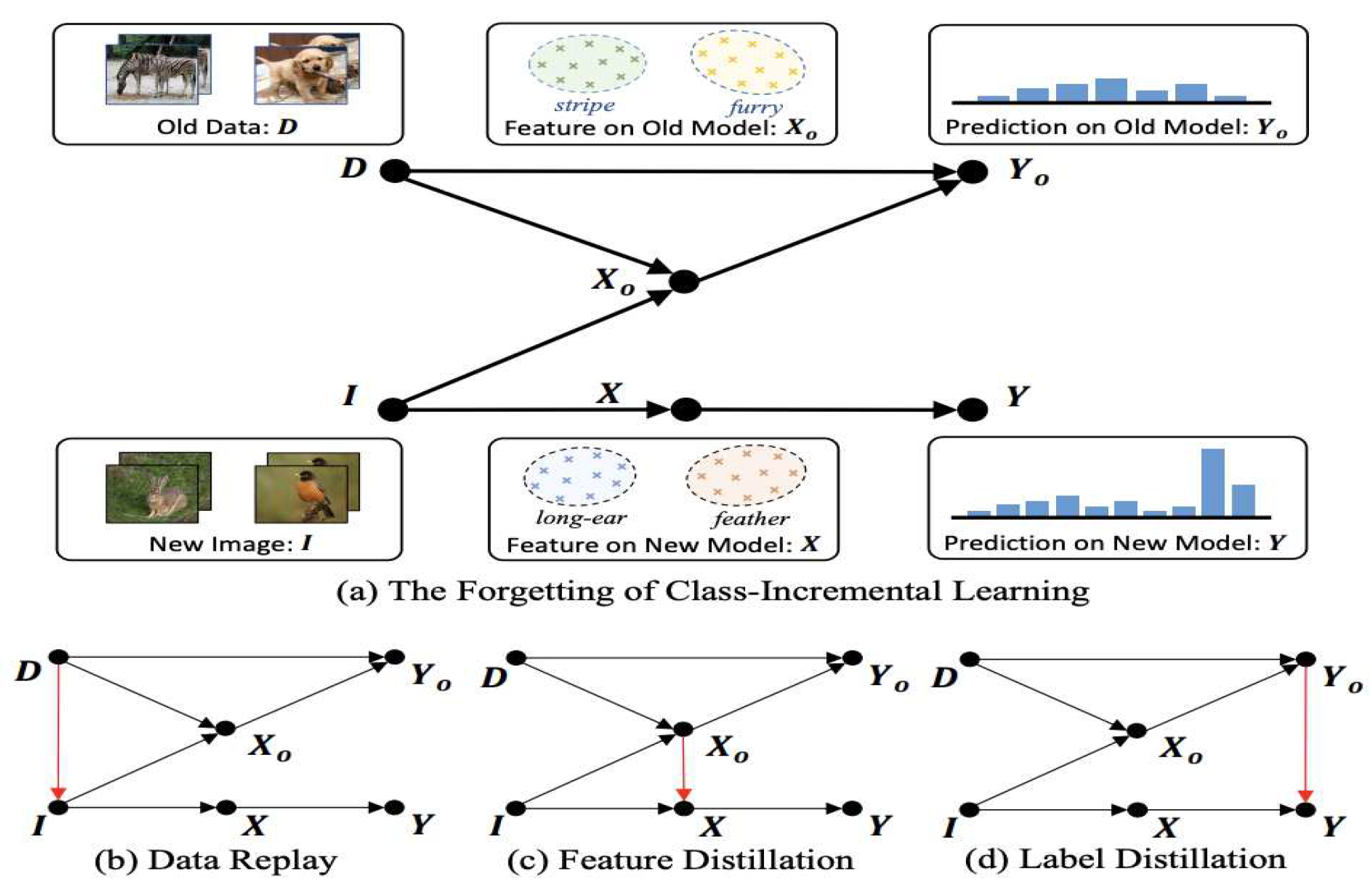
Figure 6.
Causal Graph: Confounding Effect of Background Features.
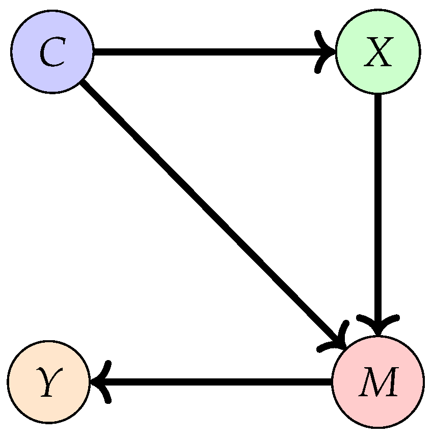
Table 1.
The table presents a hierarchy of causal reasoning in the context of computer vision, specifically for the task of dog detection. For the “Association” level, we are looking at the probability of dog detection given an image with grass in the background. Here, the grass is a correlated feature often present in the training data, but it is not causally related to the presence of a dog. For the “Intervention” level, we consider the probability of dog detection when we intervene by changing the background to a neutral colour, thereby isolating the causal features (the dog) from the non-causal ones (the background). Finally, for the “Counterfactual” level, we ask a hypothetical question: If the network failed to detect the dog without the removal of the non-causal background, would the dog have been detected if the background was removed? This allows us to determine the causal effect of the background on the dog detection task.
| Level | Symbol | Activity | Typical Question | Example | Machine Learning |
|---|---|---|---|---|---|
| Association | Seeing | What is the probability of Y given X? | Dog detection given grass in the image. | Supervised / Unsupervised Learning | |
| Intervention | Doing | What if I do X? | Dog detection given background removal. | Reinforcement Learning | |
| Counterfactual | Imagining | What if I had acted differently? | Dog detection if the background wasn’t removed? |
Disclaimer/Publisher’s Note: The statements, opinions and data contained in all publications are solely those of the individual author(s) and contributor(s) and not of MDPI and/or the editor(s). MDPI and/or the editor(s) disclaim responsibility for any injury to people or property resulting from any ideas, methods, instructions or products referred to in the content. |
© 2023 by the authors. Licensee MDPI, Basel, Switzerland. This article is an open access article distributed under the terms and conditions of the Creative Commons Attribution (CC BY) license (http://creativecommons.org/licenses/by/4.0/).
Copyright: This open access article is published under a Creative Commons CC BY 4.0 license, which permit the free download, distribution, and reuse, provided that the author and preprint are cited in any reuse.


