ARMOSA Model Parametrization on Winter Durum Wheat Cultivation under Diverse Cropping Management Practices in Mediterranean Environment

Preprint

Article

ARMOSA Model Parametrization on Winter Durum Wheat Cultivation under Diverse Cropping Management Practices in Mediterranean Environment

Altmetrics

Downloads

Views

Comments

A peer-reviewed article of this preprint also exists.

Submitted:

28 December 2023

Posted:

28 December 2023

You are already at the latest version

Alerts

Abstract

In view of the expected climate changes, a paradigm shift in soil management, through reduced tillage and/or a different use of crop residues, can be a key point in the mitigation of the climate impacts. The transition from a traditional cropping system (i.e., durum wheat in continuous cropping system under conventional tillage and/or straw removal) to those undergoing the conservative practices require to be evaluated in a medium to long time frame to reach an equilibrium and thus to be properly investigated. In this regard, cropping system simulation models are fundamental tools for the in-silico evaluation of the response of crop growth and soil organic matter dynamics to varying cropping scenarios. This paper reports the evaluations on the parameterization and reliability of the ARMOSA crop simulation model calibrated and validated on experimental datasets collected on durum wheat grown in continuous cropping system under several straw and soil management strategies in a Mediterranean environment.

Keywords:

Subject: Environmental and Earth Sciences - Environmental Science

1. Introduction

Globally, cereals are the main source of food supply for humans. The European Union is the largest producer of wheat [1]. In Italy, the production of durum wheat plays a fundamental role in the food industry. Italy is the second highest-producing country in the world of durum wheat after Canada. The total annual production of durum wheat is 4.2 million tons and is concentrated in southern Italy and the Islands with 65.6% [2].

Global warming (GW) is the principal cause of the rise of the average temperature, the reduction of rainfall, the increase of the severity and frequency of drought and floods events, and the carbon dioxide concentration in the atmosphere [3-5].

Thus, it is necessary to provide strategies to adapt and mitigate the effects of GW on crop yield and product quality. Adaptation strategies aim to minimize the negative effects of GW on agricultural production, while mitigation strategies aim to reduce greenhouse gas emissions, maintaining or increasing the organic carbon content in soil. Then, integrated analyses are necessary to adapt the cropping systems to the mutated climate conditions, in areas with homogeneous agronomic and pedo-climatic characteristics, such as the Mediterranean basin.

Nowadays, all of the above-mentioned issues caused from the GW adversely affects yields of wheat in many lower-latitude regions, while they have increased in many higher-latitude zones, during the recent decades [6].

Projections at the global level confirm this trend [7]. On the other hand, literature reports limited information concerning to the impacts of GW on production in Italy, mainly resulting from analyses of continental or global scale [7-9]. In any case, the use of accurate climate data is essential, especially in areas with high pedo-climatic and topographical variability, such as Italy [10].

Recently, in the province of Foggia (Northern Apulia), durum wheat is often grown in rotation of two or three years with tomato (two years of wheat and one of tomato) and/or with irrigated high-income crops. Traditional agronomic practices include the use of mould ploughing and additional tillage operations, such as harrowing. Straw and stubble, after being chopped, are buried in the ground by ploughing or, alternatively, are burned in early September and then ploughed and incorporated into the soil [11].

Field experiments aiming at the evaluation of the soil organic matter dynamics and crop yield in response to tillage are typically expensive and time consuming. A viable solution to overcome this limitation is the use of properly calibrated and validated process-based models to evaluate the impact of different soil and crop management practices on crop productivity and water–nutrients dynamics. Model application helps identify the most suitable management according to the pedo-climatic conditions [12-15].

In literature, there are studies testing different practices of soil and crop management of conservation agriculture (CA) on crop growth and yield, and nutrient and water dynamics in the soil-water-atmosphere system under different agro-environmental conditions [16-17]. However, most of the simulation models tested in the last years are not capable to depict the long-term effects of differences between CA practices, such as no-tillage (NT) and minimum tillage (MT), and traditional cropping managements [18].

Combining process-based crop modeling with climate data and weather projections is critical to gaining knowledge about the effects of climate change caused by global warming on agricultural production and identifying the most appropriate crop management strategies. In this way, crop modelling could provide information on mitigations and adaptations to climate change by recognizing appropriate CA practices [17, 19-20]. ARMOSA is a process-based cropping system model suitable for field crops and for simulating different soil-management practices under diverse environmental conditions [15, 21-22]

The purpose of this work was the definition of a correct crop management aimed at preserving and/or increasing soil fertility, stabilizing durum wheat yields over time, thanks to the choosing and the application of appropriate and adequately calibrated models. Therefore, ARMOSA crop simulation model was calibrated using a dataset collected along a long-term experiment (LTE) of durum wheat in continuous cropping system, cultivated in Foggia (Southern Italy) since 1977 to date under several straw practices contemplated for CA. Reliability of ARMOSA was assessed by validation step on a different LTE dataset used for ARMOSA parametrization, carried out at the same experimental farm and under two different tillage options (NT and MT).

2. Materials and Methods

2.1. Experimental field

All the field experiments were carried out in Podere 124 (P124) experimental station, located in Foggia, Apulia region, Southern Italy (latitude, 41°88’7’’N; longitude, 15°83’05’’E; altitude, 90 m a.s.l.), in two experimental parcels: P124_P30 used to calibrate the model, and P124_P32 used to validate it.

The soil, a vertisol of alluvial origin [23], is classified as silty-clay with the following physicochemical properties: 48.5% clay, 38.7% silt, 12.8% sand, bulk density 1.11 t m^-3, organic matter: 2.1%; total N: 0.122%; NaHCO₃-extractable P: 41 ppm; NH₄OAc extractable K₂O: 1598 ppm; pH: 8.3; field capacity water content: 0.396 m³ m^-3; permanent wilting point water content : 0.195 m³ m^-3; available water: 202 mm m^-1.

The climate is classified as “accentuated thermo-mediterranean” [24], characterized by temperatures below 0 °C in winter and above 40 °C in summer, with an annual average of 550 mm of rainfall, mostly concentrated in winter months [11]. The daily meteorological data of temperature, humidity, rainfall, wind parameters and solar radiation were recorded in the meteorological station located at P124.

2.2. LTE data-sets

LTE dataset used to parametrize ARMOSA and to check the robustness and reliability of the model , consisted of winter durum wheat in continuous cropping system since 1977, submitted to three different straw management and namely: i) chopping and incorporation of crop residue into soil with ploughing (T2); ii) chopping, supply of 150 kg of mineral nitrogen per hectare on straw and incorporation of crop residue into soil with ploughing (T5) and; iii) chopping, supply of 150 kg of mineral nitrogen per hectare and of 500 m3 ha-1 of irrigation water on straw and incorporation of crop residue into soil (T8).

The experimental design was arranged in a randomized block design with five replications of 8 m x 10 m cropped area and a spacing of 15 cm (between two rows) x 5 cm (on the rows) for each replication, placed in one experimental plot (area of 3500 m²) here named P_30.

For all experimental treatments, sowing, which took place in the first half of November, was preceded by fertilization with superphosphate (100 kg P₂O₅ ha^-1) plowing (with soil incorporation of the chopped straw), harrowing with the disc harrow and tilling with the rotary tiller. 100 kg N ha^-1 was supplied to the crop as top dressing in the first half of March and the harvest was performed in the middle two weeks of June.

Before harvesting, plant samples taken over an area of 2 m² was collected to estimate the total above dry biomass (TDM), placing the sample in a ventilated oven at 78 ° C, until a constant weight was reached.

The harvest wheat took place with the support of a plot combine, which determined, thanks to a portable module, grain yield for each replication and the related moisture (from which the dry weight of grain was calculated).

In addition, from 1983 to 2009, the soil organic carbon content (TOC; kg ha^-1; 0-40 cm depth) was determined discontinuously on three soil samples of about 500 gr each for each replication.

In P_30 the following cultivars (cvs) succeeded each other over the harvesting years: Valgeraldo 1978-1982, Appulo 1983-1987, Latino 1988-1992, Appio 1993-1996, Simeto 1997-2000 and 2007-2013, Ofanto 2001-2006, Claudio 2014-2018, Saragolla 2019-2021.

Consistency of ARMOSA was probed on a separate dataset applied on the parameterization process. Here, figures were gathered on another LTE consisting of the wheat in continuous cropping system since 2003, cultivated under two CA schemes NT and MT.

The experimental design was planned in the randomized block design with three replications for each treatment with an area extension of 500 m2 (20 m x 25 m) arranged in one experimental plot (P_32) with a total surface of 4450 m2.

NT provided for sowing (in the first half of November) with the no-tiller seeder and without further disturbance of soil.

Under MT, a single field operation before sowing, was performed by the combined farm device with subsoiler and rotary cultivator disturbing the first layer of soil at 0-0.10 m depth.

For all soil management, straw and stubble were chopped after harvest and spread back.

Mineral nitrogen fertilization was split in two doses, as basal dressing before sowing in the form of di-ammonium phosphate (36 and 92 kg ha^-1 of N and P₂O₅, respectively) and ammonium nitrate as top dressing (68 kg ha^-1) in the first half of March. Weed was kept under control by chemicals applied at pre-sowing and post-emergence.

The experimental design was structured in the randomized block design with three replications for the two treatments with of an area extension of 500 m2 (20 m x 25 m) arranged in one experimental plot (P_32) with a total surface of 4450 m².

The cvs that followed one another over the years in P_32 was: i) Simeto, from 2003 to 2010; ii) Claudio, from 2011 to 2018 and iii) Saragolla from 2018 to 2020.

As for P_30, the plot harvester collected data about grain yield and moisture (dry weight of grain was calculated accordingly) for each replication, over a period from 10 June to 25 June of the examined growing seasons.

Even for P_32, TOC (0-30 cm depth) from 2002 to 2020 (not continuously) was determined on three soil samples of about 500 gr each for each replication.

At emergence, flowering and physiological maturity stage verified in the experimental plots of P_30 and P_32, were associated the related calendar days (specific for each growing season, but common to all cvs). Thermal sum (°C) was computed for the specific phenological stage, accordingly.

2.3. The ARMOSA model

ARMOSA is a cropping system model that simulates crop and soil related variables at a daily time-step as affected by pedoclimatic conditions and agronomic management. The software is written in Java and structured with a high level of modularity. The model simulates the water balance, the evapotranspiration, and the N and C cycling in the soil layers, and the crop development and growth. The soil properties (i.e., texture, bulk density, initial soil organic carbon) are set for each layer of the profile. The water dynamic is simulated with the bucket approach with travel time [25].

The reference evapotranspiration is estimated using the Penman-Monteith, Priestley-Taylor, or the Hargreaves equation. Crop evapotranspiration is estimated using the FAO 56 approach [26], and the actual evapotranspiration is based on the water stress factor [27], which also affects the dry matter production and partitioning.

The simulation of crop growth and development follows the WOFOST approach [28] with two substantial differences: (i) the canopy being divided into 5 layers with different light interception and (ii) the development being described with the BBCH scale. Carbon and nitrogen related processes are simulated similarly to the SOILN model [29] with some improvements due to the fact that each input of organic matter is simulated independently according to a specific decomposition rate, C and N concentration, and soil depth incorporation. Required input data: daily weather data, soil properties (texture, bulk density, SOC, with the option to enter the measured water retention parameters), cropping system information (i.e., crop type and rotation, sowing and harvesting dates), data on fertilizers (i.e., mineral or organic, amount, timing, application depth, carbon to nitrogen ratio, ammonia and nitrate content), irrigation (i.e., water amount, timing, automatic irrigation as a function of water depletion threshold), tillage and crop residues management.

The effect of tillage is simulated as a function of tillage type (depth, degree of soil layers mixing and perturbation) as reported in the WEPP model [30]. As reported in [22] the mixing of two or more adjacent soil layers causes pools (either inorganic or organic) and state variables (e.g., soil water content) mixing. The tillage operation determines an increase in the mineralization rate of the organic carbon pools as it increase the microporosity, in agreement with [31]. Soil hydrological parameters of the water retention curve are daily computed as a function of the daily values of bulk density and soil organic carbon. The decomposition of the crop residues is simulated according to the specific decomposition rate and amount of the biomass that remains into the soil at the harvesting date (percentage of the simulated biomass of the crop organs, leaves, stem, roots).

2.3. The ARMOSA model

To adapt the predictive algorithms of durum wheat growth implemented in ARMOSA to the data harvested in LTE, the adjustment of the crop coefficients was assessed according to the "trial and error" procedure, to reflect reasonable simulations or to approach the model output closer to the observed data. Calibration of ARMOSA was conducted firstly for nitrogen and carbon cycling and then for crop growth and development, using the genetic simplex method according to [32].

The selection of parameters to calibrate was performed through the screening method of Morris modified by [33].

According to this sensitivity analysis, the mineralisation rates of the soil organic matter fractions (litter and stable pools) and the parameter PCO2 and GDD from emergence to flowering were calibrated separately for the cvs. Maximization of the Nash-Sutcliffe modelling efficiency NSE [34] was chosen as the objective function, where first the NSE for data of simulated and observed SOC were maximized and second the NSE for observed and simulated yield data, separately for the cvs.

Test bench for calibrating ARMOSA was T2, on which the model was primarily modeled. Afterward, a fine tuning of crop parameters was further implemented to approach the model outputs as closely as possible to the collected data in LTE also for T5 and T8, as well as T2.

After calibrating ARMOSA, its reliability in replicating the growth of cvs and TOC dynamic was assessed by means of appropriate evaluative indices:

R M S E = \sqrt{\frac{\sum_{= i}^{n} {(X_{o b s, i} - X_{m o d e l, i})}^{2}}{n}}

where:

RMSE is the Root Mean Square Error or the measure of the difference between values predicted by a model and the values actually observed from the environment that is being modeled [35];

Xobs,i is the observed value;

Xmodel,i is the forecast value.

G S D = \frac{R M S E}{{\bar{X}}_{o b s}}

where:

GSD is the General Standard Deviation and it can be interpreted as a fraction of the overall range that is typically resolved by the model [36];

{\bar{X}}_{o b s}

is is the average of observation value.

E F = 1 - \frac{\sum_{= i}^{n} {(X_{o b s, i} - X_{m o d e l, i})}^{2}}{\sum_{= i}^{n} (X_{o b s, i} - {\bar{X}}_{o b s})}

where:

EF is the Nash-Sutcliffe efficiency [37], a normalized statistic that determines the relative magnitude of the residual variance compared to the measured data variance;

d = 1 - \frac{\sum_{= i}^{n} {(X_{o b s, i} - X_{m o d e l, i})}^{2}}{\sum_{= i}^{n} {(|X_{m o d e l, i} - {\bar{X}}_{o b s}| + |X_{o b s, i} {\bar{X}}_{o b s}|)}^{2}}

where:

d is the Index of agreement [38].

The index of agreement can detect additive and proportional differences in the observed and simulated means and variances.

C R M = 1 - \frac{\sum_{= i}^{n} X_{m o d e l, i}}{\sum_{= i}^{n} X_{o b s, i}}

where:

CRM is the Coefficient of Residual Mass [39] that can assume positive values indicating an underestimation of the model outcome, negative values if there is an overestimation of the model output while values close to zero indicate the absence of trends.

For each evaluation index, a score ranging between -1 (worst) and 1 (best) was assigned, 0.5 for the middle one.

G S D = \{\begin{matrix} 1 i f 25 > G S D > 0; \\ 0.5 i f 25 < G S D < 40; \\ - 1 i f G S D > 40. \end{matrix}

E F = \{\begin{matrix} 1 i f 1.0 > E F > 0.4; \\ 0.5 i f 0 < E F < 0.4; \\ - 1 i f E F < 0. \end{matrix}

d = \{\begin{matrix} 1 i f 1.0 > E F > 0.7; \\ 0.5 i f 0.4 < E F < 0.7; \\ - 1 i f d < 0.4. \end{matrix}

C R M = \{\begin{matrix} 1 i f 0.01 > C R M > - 0.01; \\ 0.5 i f - 0.1 < C R M < 0.1; \\ - 1 i f 0.1 < C R M < - 0.1. \end{matrix}

The comparison by means of these indices was carried out on the specific phenology for date of emergence, flowering and physiological maturity dry biomass at harvest and grain yield and TOC.

To rank the abovementioned valuation indices, was implemented less stringent criteria than those reported by others modeling exercises [40, 41]. The authors, indeed, performed comparison between observed and simulated dataset on a specific growing season and single cvs, which are less treacherous than calibration on multiple growing years and/or cvs.

The distinct inquiry of the four evaluative indexes implied a struggle in expressing a quick and easy to read verdict of ARMOSA's performance. Accordingly, a conclusive evaluation based on the aggregation of the scores related to single indicators (-1, 0.5 and 1), was implemented.

This final score ascribable to the reliability of ARMOSA in replicating the wheat growth and productivity, assumed the following criteria: i) Very good = total score from 3.5 to 4; Good = total score from 2.5 to 3; Fair = total score from 1.5 to 2; Bad = total score from 0 to 1

The robustness of the model tested by validation step was assessed investigating the parameters of the 1: 1 regression model (i.e., R2, angular coefficient (β) and significance of the regression model) applied on yield and TOC of P_32.

3. Results and discussions

3.1. Calibration

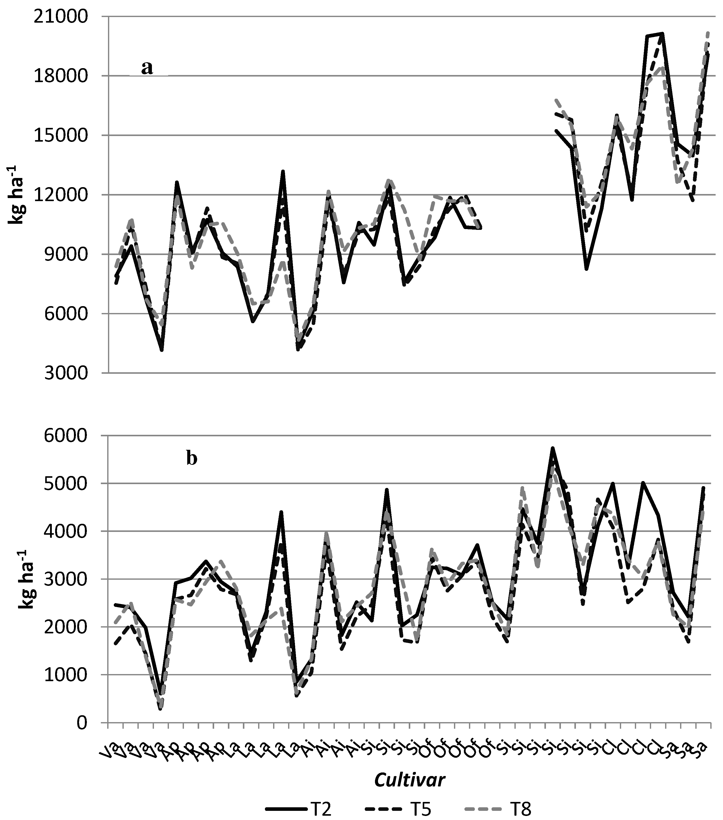
The growth and productivity of wheat showed a high variability both among cvs and across the growing seasons sown with the same cvs (Figure 1a and Figure 1b).

Valgerardo and Latino were characterized by a remarkable reduced growth in some years with negative consequences on productivity. Indeed, for Valgerardo, dry biomass accumulation stopped at values ranging between 4157 kg ha^-1 (T5) and 5447 kg ha^-1 (T8), in 1982. The grain yield behaved accordingly, with values well below 1000 kg ha^-1 for all straw treatments.

The following year, a storm that occurred just before harvest caused lodging of the plants resulting in loss of grain. Thus, data from this year were excluded from the modelling exercise here reported.

For Latino, dry biomass and productivity at harvest in 1992, remained below 5000 kg ha^-1 and 1000 kg ha^-1, respectively.

A fair stability of growth and productivity over the growing years was achieved by Ofanto and Appulo, with comparable values in terms of TDM (slightly higher than 10000 kg ha^-1 for both) and grain yield (around 3000 kg ha^-1).

Simeto and Claudio were the cvs that showed the greatest yield potential, as evidenced by the high productivity in some l years (with peaks of over 5000 kg ha^-1) when compared to the remaining cvs.

However, even for these two cvs, some growing seasons proved to be critical for the growth and accumulation of biomass with limited grain yield which for Simeto fell below 2000 kg ha^-1.

Ultimately, Saragolla was the cv that provided some of the highest (4508 kg ha^-1 in 2021; T2) and lowest yield values (1692 kg ha^-1 in 2020; T5) even if for the worst performances, the corresponding TDM was not so bad (from 11723 kg ha^-1 to 13974 kg ha^-1).

As for Valgerardo, a storm that occurred shortly before harvesting, heavily compromised the grain harvesting in 2001 (cv Ofanto) and 2018 (cv Claudio for T2 and T5 treatments); thus, the wheat data of these growing seasons were not taken into consideration for model parametrization.

The calibrated values achieved by “trial and error” procedure for the coefficient of parameters underlying the crop growth, concerned: i) the assimilation of CO₂; ii) conversion into biomass; iii) separation in the various organs of the plant; iv) development of the canopy and intercepted radiation; v) root length; vi) senescence (Table 1 and Table 2).

In addition to these parameters, the coefficients of algorithms governing the simulation of evapotranspiration (Table 2), specific partitions for each phenological phase (Table 2) and degree days (GDD; Table 3) to achieve the phenological stages were also modified.

For the emergence, flowering and maturity stages, an excellent match between the observed and simulated data was reached, both in terms of similarity of values averaged for all growing seasons and in the inter-annual variability (Table 4).

Accurate calibration of crop phenology is considered the primary, basic step in the application of crop simulation models [42]. In our modelling exercise, emergence and flowering stages of wheat as formalized by ARMOSA, attained the highest scores, the latter being capable to capture both the averaged GDD to reach these phenological stages and variability across years.

GDD to reach maturity stage was well formalized by ARMOSA, slightly penalized by the low score of EF and the middle score of d, but well depicted by GSD and CRM figures.

The better the accuracy of a simulation model in replicating the crop phenology, the greater the ability of the same framework to capture the genetic variability underlying canopy development and biomass accumulation [43].

The accumulation of biomass is related to the amount of radiation intercepted by the leaf surface which in turn is responsible for the conversion of the assimilated CO₂ into carbohydrate which is a cultivar specific trait.

In the light of this, the coefficients of some algorithms underlying the development and senescence of the canopy, the conversion of CO₂ into dry matter, maintenance respiration and water and temperature stresses for each cultivar were changed to best fit the simulation of biomass accumulation with that gathered in LTE (see Table 1).

As for phenology, the calibration phase showed the goodness of ARMOSA in faithfully replicating the total dry biomass at the harvest averaged for all soil treatments (Table 5).

Indeed, the highest score was for three out of four evaluation indices, with only a negligible deviation of GSD from the optimal value (25.77% vs 25%). By assessing the response of ARMOSA for the cropping systems separately (T2, T5 and T8), the brilliant match between observed TDM and the model output for T2 and T8 came out, with a narrow deviation from the optimal value of GSD for the former and a slight overestimation of the model for the latter. Anyway, even the response of ARMOSA in replicating T5 could be deemed satisfactory with the best performance for EF and d, but with a slight overestimation and deviation of the simulated data compared to the observed one.

The environment (Mediterranean climate) of the area under investigation is characterized by erratic pattern rainfall whit prolonged conditions of drought especially during the spring-summer period during the spring-summer period with high rainfall. Furthermore, for durum wheat cropped in Mediterranean area, the common agronomic practices do not provide for irrigation. The sum of these conditions subjects the crop to extremely variable water supply and water stress among the years and within the same growing season [44-46].

By examining the ratio between standard deviation and the mean value of TDM, it emerged that some cvs were more susceptible to climatic erraticism (i.e., Valgerardo, Latino, Appio) than others (Ofanto and Appulo; Table 6).

So, a meticulous calibration of the crop coefficients related to the adaptative mechanisms to temperature and rainfall pattern and any water / temperature stresses (i.e. WSPar, TmaxCO2, TOffCO2, KET) was performed for each cv.

On 8 cvs, ARMOSA was able to accurately replicate TDM at the end of growing season for 4 of them, fairly good for 3 cvs and only for one cv the simulation was not satisfactory.

It should be noted that for Saragolla, we investigated only 3 growing seasons (from 2019 to 2021) and this led to a reduced number of observations not adequate to optimize ARMOSA's response for this cv.

Simeto and Valgerardo resulted the cvs for which ARMOSA accurately simulated both the inter-annual variability and the average TDM observed in the field, with a slight overestimation for Simeto.

For the remaining cvs there was a mixed response; for some of them ARMOSA was efficient in replicating the biomass accumulation at harvest, returning negligible differences between the observed and simulated mean data, but less effective in capturing the variability between the various years (see GSD, EF and d for Appulo, Claudio and Ofanto).

For other cvs, the simulations comprehensively caught the inter-annual variability (i.e., Claudio and Latino) but overestimated or underestimated the average trend of TDM.

The cropping systems carried out in LTE, were characterized by the release of straw and their incorporation into the soil, differentiating for the supplement or not of nitrogen and water.

Definitively, by analysing the response of ARMOSA in simulating TDM at harvest, it emerged as the calibration process correctly trained the cropping system model to effectively replicate the data observed in the field across LTE under P_30 treatments.

Thus, the correct estimate of TDM by ARMOSA and therefore of biomass incorporated in the soil was the first key point for an adequate simulation of TOC dynamic.

In previous studies ARMOSA was calibrated and validated on a wide range of climate and soil conditions throughout Europe, conventional systems, and CA simulating TOC dynamics with very good or even excellent results (Valkama et al., 2020).

Thus, the calibration step for the TOC dynamic focused only on two parameters controlling the evolution of soil organic matter, namely Khumus (1.4*10^-4) and CMicrobEfficiency (0.4), leaving all the other parameters unchanged.

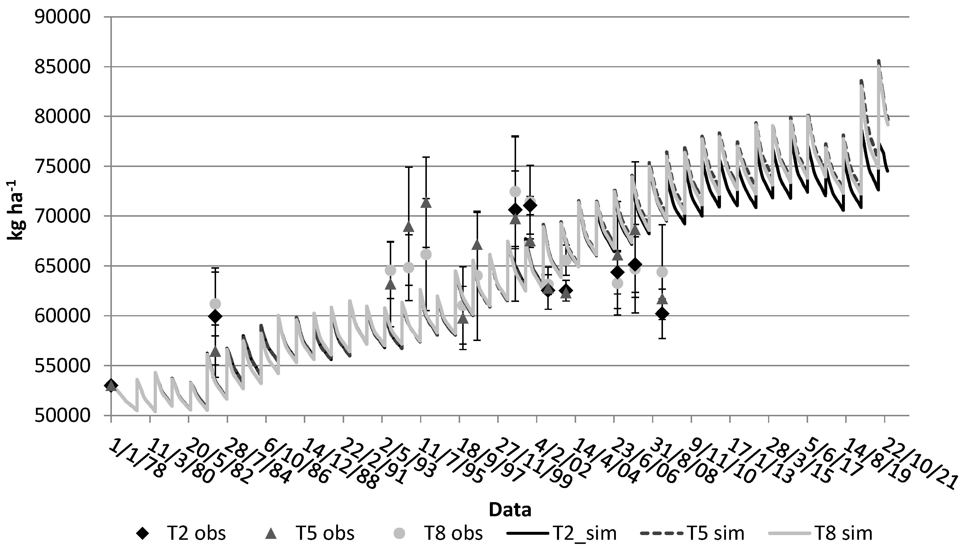
ARMOSA replicated the dynamics of TOC quite agreeably, attaining the "Good" score for all the treatments under investigation (Table 7; Figure 2). This result was reached thanks to the accurate estimate of mean value of TOC (averaged for all treatments; 64965 vs 64758 kg ha^-1, Table 7).

Although CRM index indicated a perfect alignment of the simulated values with the measured ones, it should be noted that ARMOSA tended to slightly underestimate the data collected in the initial course of LTE and then overestimate the data in the central part of LTE (Figure 2).

It was not possible to measure the robustness of ARMOSA in formalizing TOC dynamics of in the last part of LTE because of the lack of soil sampling, which instead occurred in the validation phase (see in the next section).

The high variability of the measured TOC both between consecutive years and within the same sampling (high standard deviation) is highlighted (Figure 2).

The source of this erraticism could derive from a series of conditions associated to the sampling time and sampling point. The sampling dates over the years occurred between the beginning of September and the end of November; in this period straw could still be intact (i.e., early September) or already partially degraded (i.e., late November), state also related to the moment of their burial with respect to the soil sampling. This could affect the amount of organic matter and organic carbon in the shallow layers of soil as well as the sampling point which could be affected by the substantial content (and dynamic) of crop residues [47].

This may explain the reduced matching between the measured and simulated variability of TOC (low EF and d score), although AROMSA formalized a high variability of this variable between the beginning and the end of growing period (due to the degradation dynamic of straw).

Contrasting results were obtained in the simulation of the grain yield (Table 8).

Although the total score of yield simulated averaged for all treatments was "Fair", only for T2 was achieved a good result, while for the other two treatments the outcome was not adequate.

This pattern was consequently confirmed also for the simulated yield of the several cvs. Out of 8 cvs, half did not achieve a satisfactory score, three obtained a fairly good score and only one reached the maximum score (Table 9).

GSD ranged from a minimum of 24.45% for Latino to a maximum of 66.51 % for Claudio. The latter had a low fitting in the calibration test with EF (-9.93) and CRM (-0.23), which were the worst among the simulated varieties. Apart Latino, calibration of Simeto allowed to reach satisfactory performance in terms of EF (0.1) and d (0.77), followed by Valegerardo (0.18 and 0.83 for EF and d, respectively).

The poor result of Saragolla should also be shown, with EF and d far from the optimum values, even if simulation of the mean yield was aligned with the observed data (CRM of 0.03).

Calibration of ARMOSA was focused on the parameters controlling the partition of the biomass between the different organs, therefore the grain and the maintenance respiration of the same (Table 2).

The observed data showed that grain yield was not linearly related to the biomass produced at harvest.

Several authors achieved poor performance when calibrating crop simulation models on wheat yield across different sites, years and cultivars, especially in hot-arid environments.

Specifically, some authors claimed that the grain production depends on genetic coefficients that are not only site-specific [48] but also year-specific [49-50].

Our results after the calibration of ARMOSA confirm what was reported by [51] who stated that it was difficult to accurately predict the production of wheat with low levels and / or in environments characterized by high temperatures.

The simulation of grain production becomes pernicious when situations of water and / or thermal stress occur during seed formation [52].

In the climatic condition of the experimental site of LTE, there are frequent situations of low rainfall and heat waves that have heavily compromised the potential productivity of the crop. Not to mention short but intense storms and strong gusts of wind that led to the lodging of the crop.

These extreme events which occur during seed filling, which significantly impact the final yield are hardly formalized by crop growth simulation models [53].

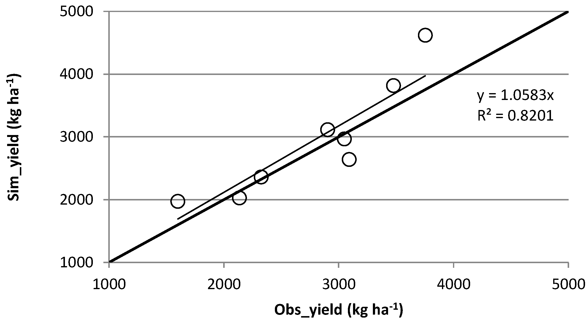
However, the 1:1 regression line between observed and simulated data (Figure 3) showed the good aptitude of ARMOSA in capturing the variability of the average grain yield among cvs (Table 8), with R2 of 0.82 and angular coefficient of 1.06.

3.1. Validation

The good robustness of ARMOSA in the simulation of phenology was also confirmed in the validation step, with maximum scores reached for the emergence and flowering phases.

Even if formalization of maturity stage did not reach the degree of excellence (EF of -1.05 and CRM of 0.46), ARMOSA was aligned with the observed mean value (156 days vs 155 days; Table 10).

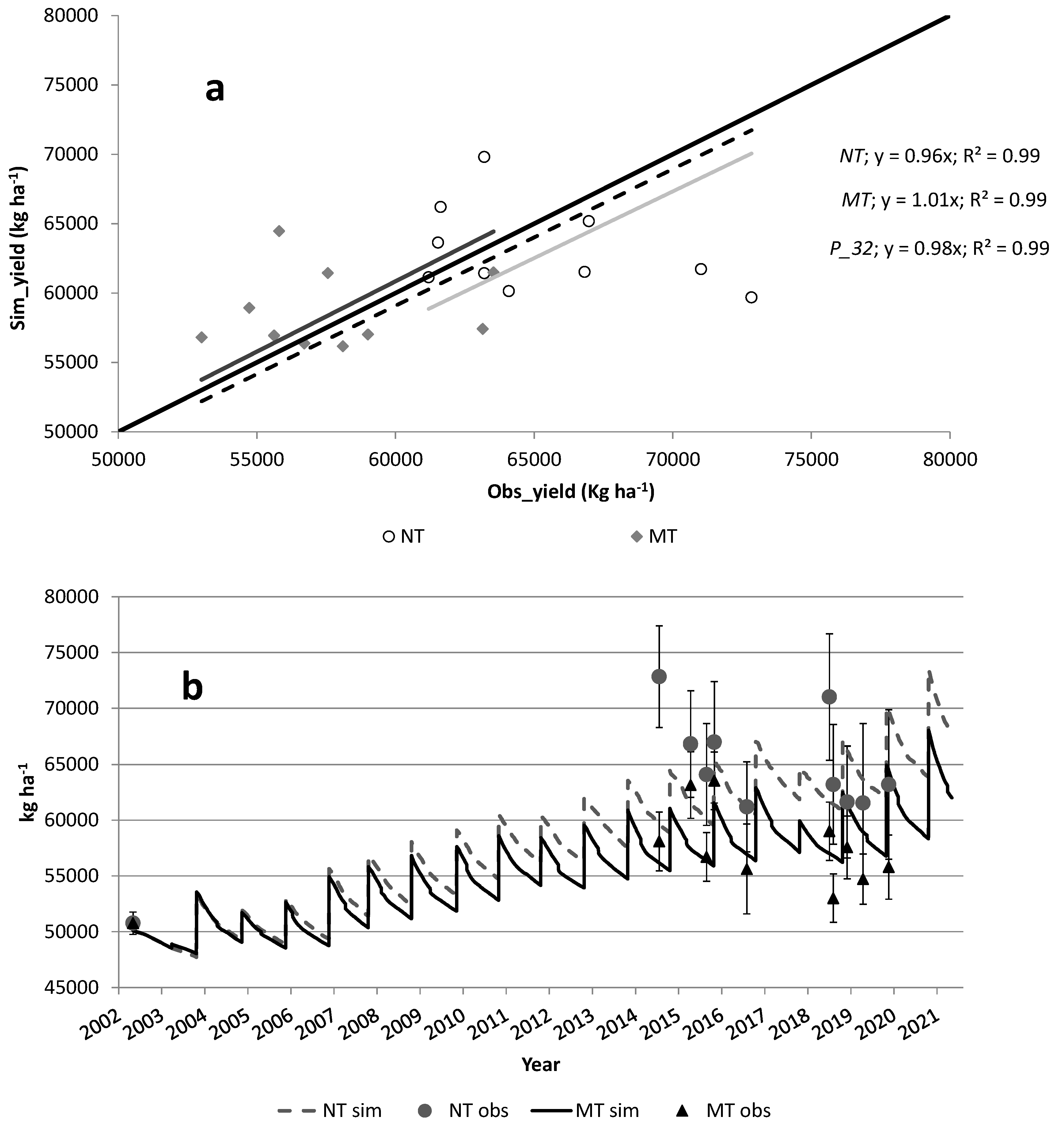
Indication on the reliability of ARMOSA in replicating the productivity of the cvs (Simeto, Claudio and Saragolla) along validation process were drawn from the results of the 1: 1 regression (Figure 4a; Table 11).

The average value of grain yield of Claudio was aligned between the model output and the observed data (4300 kg ha^-1 vs 4392 kg ha^-1). Although the standard deviation was much higher in ARMOSA compared to the LTE data, the model reasonably captured the observed variability among years (see dispersion around the 1:1 regression line). What turned out to be off-scale were the outcomes related to a single growing season for NT and MT, in which the simulated values (8154 kg ha^-1, as mean) were much higher than the observed productivity (4565 kg ha^-1).

For Saragolla, ARMOSA was inclined to slightly underestimate the actual yield (β = 0.92) but with an excellent fit between simulated and observed data (R² = 0.99), even if the compared growing seasons were only two for a total of four yield productivity figures.

For Simeto, the overestimation of grain production by ARMOSA was around 24% (3267 kg ha^-1 vs 4416 kg ha^-1). As for Claudio, a very high inconsistency between the output and the actual grain yield was observed for one growing season (2349 kg ha^-1 vs 5919 kg ha^-1 as mean), but definitively Simeto proved to be the trickiest cv for ARMOSA (although not so dramatically) of validation phase.

Evaluating ARMOSA overall for NT and MT treatments, the tendency of the model to slightly overestimate (+ 10%) the observed grain productivity was highlighted, to which was added a larger variability generated by the model, as computed by the coefficient of variation (ratio between the standard deviation and the mean) which was approximately 35% for ARMOSA and 26% for LTE.

Summing up the results obtained during the testing of ARMOSA, it was shown that the model tends to slightly overestimate the yield, with a broader sensitivity in modulating the crop performance to different climate patterns (CV = 34%) with respect to the actual plant dynamics (CV = 25%).

Testing the response of ARMOSA in formalizing TOC (Figure 4b), it emerged how the model responded differently to the two soil treatments (NT and MT) and aligning the outputs with what was observed during LTE.

Indeed, in LTE, TOC went from about 51000 kg ha^-1 at the beginning of the experimental test (2002) to 63200 kg ha^-1 in NT and 55800 kg ha^-1 in MT, respectively, in 2020.

ARMOSA did not go far from the observed data, returning for 2020 TOC value of 63045 kg ha^-1 and 65247 kg ha^-1 for NT and MT, respectively.

This opposes when comparing the simulated and observed data for some of the several experimental years (i.e., 2015 and 2019), in which substantial differences were recorded among ARMOSA outputs and actual soil TOC content.

This is because TOC determined by laboratory analysis is strongly affected by the organic substance deriving from the total or partial degradation of crop residues, the content of which can be extremely variable depending on the sampling point [47].

This also explains the extreme variability of the figures (see standard deviation in Figure 4b) observed for each sampling, both in NT and MT.

In the light of that, ARMOSA can be considered reliable in the simulation of TOC fluctuation, particularly if one considers the evolution over a period long enough to capture the correct dynamics of TOC under different crop systems [54].

4. Conclusions

In this modeling exercise, ARMOSA crop growth simulation model was tested for the reliability of replicating three growing variables of durum wheat (phenology, dry biomass accumulation and grain yield) cropped under five different soil and straw options and their impact on TOC dynamics.

After calibrating ARMOSA on eight phenotypes of durum wheat, agreeable results were achieved on phenology and biomass at harvest in almost all the investigated cvs.

On the other hand, the grain simulation generated discordant results, with some cvs being replicated sufficiently well, while others scoring unsatisfactory.

The validation step to verify the robustness of ARMOSA showed that, although in some years the deviation between the simulated data and the observed ones has been high, the model has adequately captured the grain yield averaged for all the growing seasons.

Accordingly, the application of simulation models to replicate the productivity of durum wheat across several growing periods rather than single year, in hot-arid environments with low grain yield has proved challenging, as reported by various modeling investigations.

For what concerns TOC dynamic, ARMOSA proved to be suitable in replicating the average trend of soil organic carbon both in the calibration and in the validation processes. Although the variability among years was not slavishly captured by the model (also due to the extreme spatial variability of this parameter), TOC progression in the time frame concerned LTE was adequately copied.

To finalize, ARMOSA showed great potential in formalizing the growth of durum wheat cropped in Mediterranean environment under a wide range of options concerning tillage and the impact of such agronomic schemes on TOC dynamics.

Improvements would be desirable regarding the effect of heat waves and / or prolonged drought on the final grain yield.

Author Contributions

All the authors contributed equally to this work.

Funding

This research received no external funding.

Data Availability Statement

The data presented in this study are available on request from the corresponding author.

Acknowledgments

This research is part of P.S.R. 2014/2020 (Sottomisura 16.2) project funded by Puglia region, “Smart Future Organic Farm, Un metodo innovativo (monitorabile, misurabile e certificabile) di produzione biologica verso un'agricoltura a 0 emissioni di CO2" (management document July 28th 2020 n. 030_DIR_2020_00170) and “Water4AgriFood, Miglioramento delle produzioni agroalimentari mediterranee in condizioni di carenza di risorse idriche”, PNR 2015–2020”, funded by MIUR, PON ARS01_00825 “Ricerca e Innovazione” 2014–2020. The authors want to acknowledge Marcello Mastrangelo for his skillful work in laboratory analysis.

Conflicts of Interest

The authors declare that the research was conducted in the absence of any commercial or financial relationships that could be construed as a potential conflict of interest.

References

USDA. 2018. United States Department of Agriculture. Foreign Agricultural Service. World Agricultural Production. Circular Series. December 2018.
ISTAT. 2019. Istituto Nazionale di Statistica. Agricoltura e Zootecnia. http://agri.istat.it.
IPCC. 2014. Part A: Global and Sectoral Aspects. (Contribution of Working Group II to the Fifth Assessment Report of the Intergovernmental Panel on Climate Change). In Climate Change 2014: Impacts, Adaptation and Vulnerability; IPCC: Geneva, Switzerland; p. 1132. [Google Scholar]
Bird, D.N. , Benabdallah, S., Gouda, N., Hummel, F., Koeberl, J., La Jeunesse, I., Meyer, S., Prettenthaler, F., Soddu, A., Woess-Gallasch, S. 2016. Modelling climate change impacts on and adaptation strategies for agriculture in Sardinia and Tunisia using AquaCrop and Value-at-Risk. Sci. Total Environ. 543, 1019–1027. [CrossRef]
Abd-Elmabod, S.K. , Muñoz-Rojas, M., Jordán, A., Anaya-Romero, M., Phillips, J.D., Laurence, J., Zhang, Z., Pereira, P., Fleskens, L., van der Ploeg, M., de la Rosa, D. 2021. Climate change impacts on agricultural suitability and yield reduction in a Mediterranean region. Geoderma. 374, 114453. [CrossRef]
IPCC. 2019. Summary for Policymakers. In: Climate Change and Land: an IPCC special report on climate change, desertification, land degradation, sustainable land management, food security, and greenhouse gas fluxes in terrestrial ecosystems.
Rosenzweig, C. , Elliott, J., Deryng, D., Ruane, A.C., Müller, C., Arneth, A., Boote, K.J., Folberth, C., Glotter, M., Khabarov, N., Neumann, K., Pionrek, F., Pugh, T.A.M., Schmid, E., Stehfest, E., Yang, H., Jones, J.W. 2014. Assessing agricultural risks of climate change in the 21st century in a global gridded crop model intercomparison. Proc. Natl. Acad. Sci. USA 111, 3268. [CrossRef]
Ciscar, J.C. , Feyen, L., Ibarreta, D., Soria, A. 2018. Climate impacts in Europe: Final report of the JRC PESETA III project, EUR 29427 EN, Publications Office of the European Union, Luxembourg. ISBN 978-92-79-97218-8. [CrossRef]
Hristov, J. , Toreti, A., Perez Domínguez, I., Dentener, F., Fellmann, T., Elleby C., Ceglar, A., Fumagalli, D., Niemeyer, S., Cerrani, I., Panarello, L., Bratu, M. 2020. Analysis of climate change impacts on EU agriculture by 2050, EUR 30078EN, Publications Office of the European Union, Luxembourg, 2020. 1061; -3. [Google Scholar] [CrossRef]
Mereu, V. , Gallo, A., Trabucco, A., Carboni, G., Spano, D. 2021. Modeling high-resolution climate change impacts on wheat and maize in Italy. Clim. Risk Manag. 33, 100339. [CrossRef]
Ventrella, D. , Stellacci, A.M., Castrignanò, A., Charfeddine, M., Castellini, M. 2016. Effects of crop residue management on winter durum wheat productivity in a long term experiment in Southern Italy. Eur. J. Agron. 77, 188-198. [CrossRef]
Kassam, A. , Friedrich, T., Derpsch, R. 2019. Global Spread of Conservation Agriculture Global Spread of Conservation Agriculture. Int. J. Environ. Stud. 76, 29–51. [CrossRef]
Liu, S. , Yang, J.Y., Zhang, X.Y., Drury, C.F., Reynolds, W.D., Hoogenboom, G. 2013. Modelling crop yield, soil water content and soil temperature for a soybean–maize rotation under conventional and conservation tillage systems in Northeast China. Agric. Water Manag. 123, 32–44. [CrossRef]
Shafeeq, M.P. , Aggarwal, P., Krishnan, P. 2020. Modeling the temporal distribution of water, ammonium-N and nitrate-N in the root zone of wheat using HYDRUS-2D under conservation agriculture. Environ. Sci. Pollut. Res. 27, 2197–2216. [CrossRef]
Puig-Sirera, À. , Acutis, M., Bancheri, M., Bonfante, A., Botta, M., De Mascellis, R., Orefice, N., Perego, A., Russo, M., Tedeschi, A., Troccoli A., Basile A. 2022. Zero-tillage effects on durum wheat productivity and soil-related variables in future climate scenarios: a modeling analysis. Agronomy. 12, 331. [CrossRef]
Ngwira, A.R. , Aune, J.B., Thierfelder, C. 2014. DSSAT Modelling of Conservation Agriculture Maize Response to Climate Change in Malawi. Soil Tillage Res. 143, 85–94. [CrossRef]
Corbeels, M. , Chirat, G., Messad, S., Thierfelder, C. 2016. Performance and Sensitivity of the DSSAT crop growth model in simulating maize yield under conservation agriculture. Eur. J. Agron. 76, 41–53. [CrossRef]
Chaki, A.K. , Gaydon, D.S., Dalal, R.C., Bellotti, W.D., Gathala, M.K., Hossain, A., Menzies, N.W. 2022. How we used APSIM to simulate conservation agriculture practices in the rice-wheat system of the eastern gangetic plains. Field Crop. Res. 275, 108344. [CrossRef]
Matthews, R.B. , Rivington, M., Muhammed, S., Newton, A.C., Hallett, P.D. 2013. Adapting crops and cropping systems to future climates to ensure food security: The role of crop modelling. Glob. Food Sec. 2, 24–28. [CrossRef]
Corbeels, M. , Berre, D., Rusinamhodzi, L., Lopez-Ridaura, S. 2018. Can we use crop modelling for identifying climate change adaptation options? Agric. For. Meteorol. 256–257, 46–52. [CrossRef]
Perego, A. , Giussani, A., Sanna, M., Fumagalli, M., Carozzi, M., Alfieri, L., Brenna, S., Acutis, M. 2013. The ARMOSA simulation crop model: overall features, calibration and validation. Italian J. Agrometeorol. 3, 23-38.
Valkama, E. , Kunypiyaeva, G., Zhapayev, R., Karabayev, M., Zhusupbekov, E., Perego, A., Schillaci, C., Sacco, D., Moretti, B., Grignani, C., Acutis, M. 2020. Can conservation agriculture increase soil carbon sequestration? A modelling approach. Geoderma. 369, 114298. [CrossRef]
USDA. Soil Taxonomy Classification. United States Department of Agriculture, USDA 2010.
Emberger, L. 1945. Climate Biogeographic Classification.
Savabi, M.R. , Williams, J.R. 1995. Chapter 5. Water balance and percolation. In D.C. Flanagan and M.A. Nearing (eds.): USDA-Water Erosion Prediction Project: Hillslope Profile and Watershed Model Documentation. NSERL Report No. 10, National Soil Erosion Research Laboratory, USDA-Agricultural Research Service, West Lafayette, Indiana, 5.1-5.14.
Allen, R.G. , Pereira, L.S., Raes, D., Smith, M. 1998. Crop evapotranspiration - Guidelines for computing crop water requirements - FAO Irrigation and drainage paper 56, FAO - Food and Agriculture Organisation of the United Nations, Rome. http://www.fao.org/docrep.
Sinclair, T.R. , Muchow, R.C., Ludlow, M.M., Leach, G.J., Lawn, R.J., Foale, M.A. 1987. Field and model analysis of the effect of water deficits on carbon and nitrogen accumulation by soybean, cowpea and black gram. Field Crop Res. 17(2), 121-140. [CrossRef]
van Diepen, C.A. , Wolf, J., van Keulen, H., Rappoldt, C. 1989. WOFOST: a simulation model of crop production. Soil Use Manag. 5(1), 16-24. [CrossRef]
Johnsson, H. , Bergstrom, L., Jansson, P.E., Paustian, K. 1987. Simulated Nitrogen Dynamics and Losses in a Layered Agricultural Soil. Agric. Ecosyst. Environ. 18, 333–356. [CrossRef]
Flanagan, D.C. , Gilley, J.E., Franti, T.G. 2007. Water Erosion Prediction Project (WEPP): development history, model capabilities and future enhancements. Transaction of the ASABE 2007 American Society of Agricultural and Biological Engineer. 50(5), 1603-1612.
Rádics, J.P. , Jóri, I.J., Fenyvesi, L. 2014. Soil CO2 emission induced by tillage machines. Int. J. Appl. Sci. Tech. 4, 37–44.
Acutis, M. , Confalonieri, R. 2006. Optimization algorithms for calibrating cropping systems simulation models. A case study with simplex-derived methods integrated in the WARM simulation environment. Ital. J. Agrometeorol. 3, 26-34.
Campolongo, F. , Cariboni, J., Saltelli., A. 2007. An effective screening design for sensitivity analysis of large models. Environ. Modell. Softw. 22, 1509-1518. [CrossRef]
Nash, J.E. , Sutcliffe, J.V. 1970. River Flow Forecasting through Conceptual Model. Part 1—A Discussion of Principles. J. Hydrol. 10, 282-290. [CrossRef]
Fox, D.G. 1981. Judging air quality model performance: a summary of the AMS workshop on dispersion models performance. Bull. Am. Meteorol. Soc. 62, 599-609. [CrossRef]
Jørgensen, S.E., L. Kamp-Nielsen, T. Christensen, J. Windolf-Nielsen, B. Westergaard. 1986. Validation of a prognosis based upon a eutrophication model. Ecol. Model., 35, 165-182. [CrossRef]
Greenwood, D.J. , Neeteson, J.J., Draycott, A. 1985. Response of potatoes to N fertilizer: dynamic model. Plant Soil. 85, 185-203. [CrossRef]
Willmott, C.J. , Wicks, D.E. 1980. An empirical method for the spatial interpolation of monthly precipitation within California. Phys. Geogr. 1, 59-73. [CrossRef]
Loague, K. , and R.E. Green. 1991. Statistical and graphical methods for evaluating solute transport models: overview and application. J. Contam. Hydrol., 7:51-73.
Garofalo, P. , Di Paolo, E., & Rinaldi, M. 2009. Durum wheat (Triticum durum Desf.) in rotation with faba bean (Vicia faba var. minor L.): long-term simulation case study. Crop and Pasture Science, 60 (3), 240-250.
Rinaldi, M. , Garofalo, P., Rubino, P., Steduto, P. 2011. Processing tomatoes under different irrigation regimes in Southern Italy: agronomic and economic assessments in a simulation case study. J Agrometeorol. 3(3), 39-56.
Archontoulis, S.V. , Miguez, F.E., Moore, K.J., 2014. A methodology and an optimization tool to calibrate phenology of short-day species included in the APSIM PLANT model: application to soybean. Environ. Modell. Softw. 62, 465– 477. [CrossRef]
Robertson, M.J. , Carberry, P.S., Huth, N.I., Turpin, J.E., Probert,M.E., Poulton, P.L., Bell, M., Wright, G.C., Yeates, S.J., Brinsmead, R.B. 2002. Simulation of growth and development of diverse legume species in APSIM. Aust. J. Agric.Res. 53(4), 429–446. [CrossRef]
Habash, D.Z. , Kehel, Z., Nachit, M. 2009. Genomic approaches for designing durum wheat ready for climate change with a focus on drought. J. Exp. Bot. 60(10), 2805–2815. [CrossRef]
Latiri, K. , Lhomme, J.P., Annabi, M., Setter, T.L. 2010. Wheat production in Tunisia: Progress, inter-annual variability and relation to rainfall. Eur. J. Agron. 33(1), 33-42. [CrossRef]
Kyratzis, Angelos C., Pallides, A., Katsiotis, A. 2022. Investigating stability parameters for agronomic and quality traits of durum wheat grown under mediterranean conditions. Agronomy 12(8) 1774. [CrossRef]
Zhang, Z. , Sun, Y., Yu, D., Mao, P., Xu, L. 2018. Influence of sampling point discretization on the regional variability of soil organic carbon in the Red Soil region, China. Sustainability. 10(10), 3603. [CrossRef]
Gabrielle, B. , Roche, R., Angas, P., Cantero-Martinez, C., Cosentino, L., Mantineo, M., Langensiepen, M., Hénault, C., Laville, P., Nicoullaud, B., Gosse, G. 2002. A priori parameterisation of the CERES soil–crop models and tests against several European data sets. Agronomie 22, 119–132. [CrossRef]
Overman, A.R. , Blue, W.G. 1990. Estimating yields and forage N for bahiagrass production in Florida. Soil Crop Sci. Soc. Fla. Proc. 49, 113–117.
Overman, A.R. , Wilkinson, S.R., Evers, G.W. 1992. Yield response of Bermudagrass and Bahiagrass to applied nitrogen and overseed clover. Agron. J. 84, 998–1001. [CrossRef]
Timsina, J. , Humphreys, E. 2006. Performance of CERES-Rice and CERES-Wheat models in rice–wheat systems: a review. Agric. Syst. 90, 5–31.
Langensiepen, M. , Hanus, H., Schoop, P., Gräsle, W. 2008. Validating CERES-wheat under North-German environmental conditions. Agric. Syst. 97, 34–37. [CrossRef]
Dettori, M. , Cesaraccio, C., Motroni, A., Spano, D., Duce, P. 2011. Using CERES-Wheat to simulate durum wheat production and phenology in Southern Sardinia, Italy. Field Crops Res.120(1), 179-188. [CrossRef]
Monteleone, M. , Cammerino, A.R.B., Garofalo, P., Delivand, M.K. 2015. Straw-to-soil or straw-to-energy? An optimal trade off in a long term sustainability perspective. Appl. Energy. 154, 891–899. [CrossRef]

Figure 1. Trend of the total dry biomass (a) and grain yield (b) at the harvest of durum wheat following one another in the growing years for P_30. Va stands for Valgerardo, Ap for Appulo, La for Latino, Ai for Appio, Si for Simeto, Cl fro Claudio and Sa for Saragolla.

Figure 2. Comparison between simulated and observed data of TOC (0-40 cm) for P_30. Bars indicate the standard deviation.

Figure 3. Linear regression (thin line) between observed grain yield (Obs_yield) and simulated grain yield (Sim_yield) of P_30. Empty circles indicate the yield averaged for each cultivar.

Figure 4. Linear regression between observed yield (Obs_yield) and simulated yield (Sim_yield) achieved by NT (gray line), MT (thin black line), P_32 (dashed line) in the validation step (a). TOC (0-40 cm) dynamics of observed (obs) and simulated (sim) NT and MT verified across experimental years of LTE (b).

Table 1. Calibrated values of crop parameters per cultivar. Only modified values are showed in the table.

Parameter	Default value				Cultivars
		Appio	Appulo	Claudio	Latino	Ofanto	Saragolla	Simeto	Valgerardo
SPar	12	-	14	-	-	14	19	-	-
EAIfactor	0.5	-	-	-	-	0.4	-	-	-
LAITH_min	4	-	-	-	-	3	-	-	-
MaintenanceLeaves	0.05	-	-	0.01	-	-	0.02	0.01	-
MaintenanceRoots	0.015	0.05	-	0.01	-	-	0.01	0.01	0.03
MaintenanceStem	0.015	0.05	0.005	0.01	-	-	0.01	0.01	0.09
MaintenanceStorage	0.01	0.05	0.07	0.003	-	-	0.03	0.003	0.01
PARAgeD_LAI	0.3	0.08	0.7	-	0.2	0.2	0.2	0.43	-
MaxCO₂Net	1200	-	1500	-	-	-	-	-	1000
PCO₂	0.0052	-	0.015	0.003	0.001	0.004	0.0099	0.0025	0.0009
MaxRootDepth	800	-	-	900	1000	1000	-	-	-
SLA	0.017	-	0.005	-	-	-	-	-	-
T_maxCO₂	40	36	37	36	36	36	36	33	25
T_OffCO₂	40	-	-	-	-	-	-	37	36
DeathAgeingLeavesStart	60	-	-	40	40	-	-	-	-
A_crit	0.053	0.043	0.043	-	-	-	-	-	-
A_min	0.022	-	-	-	-		0.012	-	-
A_max	0.083	-	-	-	-	0.05	-	-	-
K_ET BBCH 50	1.05	-	1.1	-	-	-	0.95	-	1.1
K_ET BBCH 78	1.05	-	1.1	-	-	-	0.95	-	1.1
K_ET BBCH 97.125	0.9	-	1.85	-	-	-	0.7	-	-

Table 2. Calibrated values of plant partition parameters per cultivar. Only modified values are showed in the table.

Parameter	Default value				Cultivars
		Appio	Appulo	Claudio	Latino	Ofanto	Saragolla	Simeto	Valgerardo
FDM_Leaves BBCH 40	0.4	0.5	-	-	-	-	-	-	-
FDM_Leaves BBCH 46.905	0.4	-	-	-	-	-	-	0.3	-
FDM_Leaves BBCH 57.94875	0.4	0.3	-	-	-	-	0.3	-	-
FDM_Leaves BBCH 61	0.1	0	0.3	0.3	-	0	0.2	-	0.2
FDM_Leaves BBCH 75	0	-	0.2	-	-	-	-	-	-
FDM_Stem BBCH 0	1	-	0	-	-	-	-	-	-
FDM_Stem BBCH 40	0.6	0.5	-	-	-	-	-	-	0.5
FDM_Stem BBCH 46.905	0.6	-	-	-	-	-	-	0.7	0.5
FDM_Stem BBCH 57.94875	0.6	0.4	-	-	-	-	-	-	0.4
FDM_Stem BBCH 61	0	-	0.2	0.3	-	-	0.6	-	-
FDM_Stem BBCH 75	0	-	0.1	-	-	-	0.2	-	-
FDM_Stem BBCH 80	0	-	-	-	-	-	0.1	-	-
FDM_Storage BBCH 0	0	-	1	-	-	-	-	-	-
FDM_Storage BBCH 40	0	-	-	-	-	-	-	-	0.1
FDM_Storage BBCH 46.905	0	-	-	-	-	-	-	-	0.1
FDM_Storage BBCH 57.94875	0	0.3			-	-	-	-	0.2
FDM_Storage BBCH 61	0	1	0.5	0.4	0.9	1	0.1	0.9	0.8
FDM_Storage BBCH 75	0.9	1	0.7	1	1	1	0.6	1	1
FDM_Storage BBCH 80	0	-	-	-	-	-	0.9	-	-
FDM_Shoot BBCH 0	0.5	-	0.3	-	-	-	-	-	-
FDM_Shoot BBCH 9	0.5	-	0.3	-	-	-	-	-	-
FDM_Shoot BBCH 29.23875	0.55	-	0.5	-	-	-	-	-	-
FDM_Shoot BBCH 55.845	0.9	-	-	-	-	-	-	0.85	1

Table 3. Calibrated values of phenological stage specific parameters per cultivar. Only modified values are showed in the table.

Parameter	Default value				Cultivars
		Appio	Appulo	Claudio	Latino	Ofanto	Saragolla	Simeto	Valgerardo
GDD_sum Emergence	50	90	-	70	70	70	-	90	60
GDD_sum Tillering	400	250	-	250	350	450	300	250	200
GDD_sum Flowering	350	250	300	300	-	-	300	-	-
GDD_sum Physiological maturity	600	300	220	300	250	200	300	300	350
T_base Emergence	5	7	7	-	-	-	-	-	-
T_base Tillering	5	-	7	-	-	-	-	-	-
T_base Flowering	8	-	5	-	-	-	-	-	-
T_base Physiological maturity	8	-	6	-	-	6	7	7	-

Table 4. Comparison between observed and simulated data for the phenological stages recorded for all cultivars and treatments of P_30. Observed and simulated data of phenology was equal for all cvs. White, light gray and gray cells indicate the best (1), mid (0.5) and worst (0) scores, respectively.

Parameter	Unit	Obs	Mean		Dev.st		RMSE	GSD	EF	d	CRM	Score
		n°	Obs	Sim	Obs	Sim	(GDD)	(%)
Emergence	GDD (°C)	43	352	347	18	20	11	3.06	0.70	0.92	-0.01	Very good
Flowering	GDD (°C)	43	129	131	8	10	9	6.82	0.21	0.74	0.01	Very good
Maturity	GDD (°C)	43	158	157	9	8	9	6.01	-0.36	0.62	0.00	Good
Very good = total score from 3.5 to 4; Good = total score from 2.5 to 3; Fair = total score from 1.5 to 2; Bad = total score from 0 to 1. The same for the other tables.

Table 5. Comparison between simulated and observed data of total dry biomass and performance evaluation indices of the model applied to straw treatments. White, light gray and gray cells indicate the best (1), mid (0.5) and worst (0) scores, respectively.

Parameter	Unit	Obs	Mean		Dev.st		RMSE	GSD	EF	d	CRM	Score
treatment		n°	Obs	Sim	Obs	Sim	(kg ha^-1)	(%)
T2	kg ha^-1	36	10835	10475	± 4005	± 3076	2916	26.91	0.45	0.81	0.03	Very good
T5	kg ha^-1	36	10824	11509	± 3884	± 4303	2877	26.58	0.44	0.86	-0.06	Good
T8	kg ha^-1	37	11124	11873	±3696	± 4163	2653	23.85	0.47	0.87	-0.07	Very good
P_30	kg ha^-1	109	10930	11291	± 3829	± 3898	2816	25.77	0.45	0.85	-0.03	Very good

Table 6. Comparison between simulated and observed data of total dry biomass and performance evaluation indices of the model applied to individual cultivars. White, light gray and gray cells indicate the best (1), mid (0.5) and worst (0) scores, respectively.

Parameter	Unit	Obs	Mean		Dev.st		RMSE	GSD	EF	d	CRM	Score
cv		N°	Obs	Sim	Obs	Sim	(kg ha^-1)	(%)
Appio	kg ha^-1	12	9148	8713	± 2377	± 939	2473	27.03	-0.18	0.39	0.05	Fair
Appulo	kg ha^-1	12	10346	10706	± 1473	± 667	1625	15.18	-0.33	0.32	-0.03	Fair
Claudio	kg ha^-1	13	15911	14709	± 3792	± 3948	3368	21.17	0.15	0.79	0.08	Good
Latino	kg ha^-1	15	7393	8953	± 2607	±2546	2250	30.43	0.20	0.81	-0.21	Fair
Ofanto	kg ha^-1	12	10981	11340	± 827	± 2320	2318	21.11	-7.58	0.41	-0.03	Good
Saragolla	kg ha^-1	9	15517	17035	± 3207	± 5599	6427	41.42	-3.52	0.40	-0.12	Bad
Simeto	kg ha^-1	24	11346	11808	± 2834	± 2200	1971	17.37	0.50	0.83	-0.06	Very good
Valgerardo	kg ha^-1	12	7411	7045	± 2187	± 1953	737	9.94	0.88	0.97	0.05	Very good

Table 7. Comparison between simulated and observed data of TOC (0-40 cm) for P_30 and performance evaluation indices of the model applied to each treatment. White, light gray and gray cells indicate the best (1), mid (0.5) and worst (0) scores, respectively.

Parameter	Unit	Obs	Mean		Dev.st		RMSE	GSD	EF	d	CRM	Score
		N°	Obs	Sim	Obs	Sim	(kg ha^-1)	(%)
T2	kg ha^-1	8	66345	64549	± 5738	± 4279	6371	9.60	-0.41	0.50	0.03	Good
T5	kg ha^-1	13	64313	65060	± 5700	± 4390	6071	9.44	-0.23	0.57	-0.01	Good
T8	kg ha^-1	13	64226	65127	±5517	± 3373	5780	9.00	-0.19	0.36	-0.01	Good
P_30	kg ha^-1	34	64758	64965	± 5537	± 3883	6035	9.32	-0.22	0.48	0.00	Good

Table 8. Comparison between simulated and observed data of grain yield at harvest for P_30 and performance evaluation indices of the model applied to each treatment. White, light gray and gray cells indicate the best (1), mid (0.5) and worst (0) scores, respectively.

Parameter	Unit	Obs	Mean		Dev.st		RMSE	GSD	EF	d	CRM	Score
		N°	Obs	Sim	Obs	Sim	(kg ha^-1)	(%)
T2	kg ha^-1	40	3074	2832	± 1214	± 1382	1175	38.22	0.04	0.78	0.08	Good
T5	kg ha^-1	40	2735	3114	± 1206	± 1549	1413	51.66	-0.41	0.69	-0.13	Bad
T8	kg ha^-1	41	2902	3265	± 1116	± 1509	1411	48.62	-0.63	0.66	-0.13	Bad
Total	kg ha^-1	121	2904	3072	± 1178	± 1481	1338	46.07	-0.30	0.71	-0.06	Fair

Table 9. Comparison between simulated and observed data of grain yield and performance evaluation indices of the model applied to individual cultivars. White, light gray and gray cells indicate the best (1), mid (0.5) and worst (0) scores, respectively.

Parameter	Unit	Obs	Mean		Dev.st		RMSE	GSD	EF	d	CRM	Score
		N°	Obs	Sim	Obs	Sim	(kg ha^-1)	(%)
Appio	kg ha^-1	12	2325	2361	± 1031	± 393	1239	53.3	-0.58	0.1	-0.02	Bad
Appulo	kg ha^-1	12	2903	3114	± 306	± 353	1564	19.39	-2.72	0.23	-0.06	Fair
Claudio	kg ha^-1	13	3754	4618	± 786	± 2624	2497	66.51	-9.93	0.37	-0.23	Bad
Latino	kg ha^-1	15	2135	2029	± 1093	± 912	524	24.54	0.71	0.92	0.05	Very good
Ofanto	kg ha^-1	15	3092	2641	± 437	± 989	1066	34.47	-5.38	0.42	0.15	Bad
Saragolla	kg ha^-1	9	3049	2966	± 1293	± 1091	2095	68.71	-1.96	0.06	0.03	Bad
Simeto	kg ha^-1	33	3477	3818	± 1274	± 1292	1190	34.22	0.1	0.77	-0.10	Fair
Valgerardo	kg ha^-1	12	1600	1973	± 817	± 1044	708	44.25	0.18	0.83	-0.23	Fair

Table 10. Comparison between observed and simulated data for the phenological stages recorded for all cultivars and treatments of P_32 in the validation step. Observed and simulated data of phenology was equal for all cvs. White, light gray and gray cells indicate the best (1), mid (0.5) and worst (0) scores, respectively.

Parameter	Unit	Obs	Mean		Dev.st		RMSE	GSD	EF	d	CRM	Score
		n°	Obs	Sim	Obs	Sim	(GDD)	(%)
Emergence	GDD	14	365	368	27	35	13	3.56	0.74	0.95	-0.01	Very good
Flowering	GDD	14	123	128	7	11	10	8.13	-1.11	0.63	-0.04	Very good
Maturity	GDD	14	155	156	6	7	9	5.81	-1.05	0.46	-0.01	Good

Table 11. Comparison between observed and simulated data of grain yield in the validation step and main parameters of the related linear regression.

Parameter	Unit	Obs	Mean		Dev.st		R-squared	p-val (fit)	β	p-val (β)
		n°	Obs	Sim	Obs	Sim
Simeto	kg ha^-1	8	3267	4416	± 957	± 720	0.87	< .001	1.24	< .001
Claudio	kg ha^-1	7	4300	4392	± 617	± 2027	0.86	< .001	1.02	< .001
Saragolla	kg ha^-1	2	3089	2867	±656	± 402	0.99	< .001	0.92	< .001
NT	kg ha^-1	17	3703	4202	± 953	± 1481	0.86	< .001	1.08	< .001
MT	kg ha^-1	17	3684	4246	± 963	± 1478	0.87	< .001	1.11	< .001
P_32	kg ha^-1	34	3676	4224	± 944	± 1457	0.87	< .001	1.1	< .001

Disclaimer/Publisher’s Note: The statements, opinions and data contained in all publications are solely those of the individual author(s) and contributor(s) and not of MDPI and/or the editor(s). MDPI and/or the editor(s) disclaim responsibility for any injury to people or property resulting from any ideas, methods, instructions or products referred to in the content.

© 2023 by the authors. Licensee MDPI, Basel, Switzerland. This article is an open access article distributed under the terms and conditions of the Creative Commons Attribution (CC BY) license (http://creativecommons.org/licenses/by/4.0/).

Copyright: This open access article is published under a Creative Commons CC BY 4.0 license, which permit the free download, distribution, and reuse, provided that the author and preprint are cited in any reuse.

MDPI Initiatives

Important Links

Choose an area of interest and we will send you notifications of new preprints at your preferred frequency.

Disclaimer

ARMOSA Model Parametrization on Winter Durum Wheat Cultivation under Diverse Cropping Management Practices in Mediterranean Environment

Abstract

1. Introduction

2. Materials and Methods

2.1. Experimental field

2.2. LTE data-sets

2.3. The ARMOSA model

2.3. The ARMOSA model

3. Results and discussions

3.1. Calibration

3.1. Validation

4. Conclusions

Author Contributions

Funding

Data Availability Statement

Acknowledgments

Conflicts of Interest

References

MDPI Initiatives

Important Links

Subscribe