Detecting IoT Anomaly using Fuzzy Subspace Clustering Algorithm

There are many applications of anomaly detection in IoT domain. IoT technology consists of large number of interconnecting digital devices not only generating huge data continuously but also making real-time computations. Since IoT devices are highly exposed due to Internet, they frequently meet with the challenges of illegitimate accesses in the form of intrusions, anomaly, fraud, etc. Identifying these illegitimate accesses in IoT domain can be an exciting research problem. In numerous applications fuzzy clustering and rough set theory have been successfully employed. As the data generated in IoT domains are high-dimensional, the clustering methods used for lower dimensional data cannot be applied efficiently. In this article, mixed approaches consisting of nano topology and fuzzy clustering techniques are proposed for anomaly detection. First of all, the nano topology is generated to find lower dimensional apace and then a couple of well-known fuzzy clustering techniques are employed on it for the efficient anomaly detection. The effectiveness of the proposed approaches is evaluated using time-complexity analysis, experimental studies with a synthetic dataset and a real-life dataset along with comparative studies with traditional fuzzy clustering approaches namely fuzzy c-means clustering (FCM) algorithm, Gustafson-Kessel (GK) Algorithm, Gath-Geva (GG) Algorithm, Mahalanobis Distance based Fuzzy C-Means algorithm (M-FCM), and Common Mahalanobis Distance based Fuzzy C-Means algorithm (CM-FCM). Experimentally, it has been found that the proposed approaches outperform the aforesaid algorithms in terms of detection rates, accuracy rates, false alarm rates and computational times.

Keywords:

Subject: Computer Science and Mathematics - Artificial Intelligence and Machine Learning

1. Introduction

There is a huge applications comprising sensors that provide critical data that evolves over time, mostly as a result of the development of the IoT [1] along with their sources of real data generation. As a result, we are witnessing a rapid surge of streaming and time-series data availability. Analysing such data can yield insightful information.

The uncovering of anomaly from IoT data has substantial real-world applications across various activities such as pre-emptive maintenance, prevention of fraud, fault finding, and monitoring. Therefore, detecting anomalies can provide actionable information in the circumstances, where no trustworthy answers exist. Reliable answers to the problems are put forwarded to address the IoT anomaly.

High dimensionality typically makes it difficult to discover anomalies. Data sparsity is a result of the fact that as the features or attributes grows, more data is necessary to generalization of the detection system. These extra variables or a significant quantity of noise from numerous insignificant features, which hide the genuine outliers, are the cause of the data sparsity. The "curse of dimensionality" [3,4] is a famous term coined for the problem. Therefore, several conventional anomaly detection techniques like k-means, k-medoids, DBSCAN [5,6,7] are found to be unsuitable for such data as they fail to retain their efficacy.

In [8], the authors introduced a new concept called rough set theory, for dealing with uncertainty or vagueness existed in any real life problem. In [9], a classification algorithm based on neighbourhood rough set was proposed for the anomaly detection in mixed attribute datasets. In [10], the authors defined nano topological space of a subset X of universe U using both the approximations of X. In [11], the authors have proposed to generate CORE (a subset of attribute set) of conditional attribute set for medical diagnosis.

Clustering is a data mining technique used to unearth the distribution of data and the patterns in any datsets. Clustering has been widely applied in anomaly detection. In [12], the authors used k-means algorithm for anomaly detection approach in network traffic dataset. A fuzzy c-means clustering-based technique for anomaly detection in mixed data has been put out by the authors in [13]. In [14], the authors put forwarded a hierarchical clustering method for mixed data anomaly detection. For detecting anomalies in mixed data, in [15], a hybrid clustering strategy is proposed that combines both partitioning and hierarchical techniques. In [16], an method of finding of anomaly in high-dimensional and categorical data was proposed. Analogous researches were presented in [17,18,19,20,21,22,23,24,25,26,27,28,29]. The authors of [30] addressed the insider threat, which poses serious problems for the industrial control systems' cyber security. The authors of [31] presented an online random forest-based anomaly detection method. In [32,33,34], fuzzy techniques for real-time anomaly detections were covered. For the purpose of identifying anomay in significant cyberattacks, the authors of [35] presented a fuzzy approach based on neural networks.

The majority of the aforementioned algorithms have some limitations. Some, for instance, are ineffective at finding anomalies in high-dimensional data. In [36], the authors put forwarded a mixed algorithm consisting of a partitioning and a hierarchical approach for real-time anomaly detection which produces stable clusters along their fuzzy lifetimes. However, the algorithm [36], is not so efficient in high-dimensional data. Also traditional k-means algorithm has wide range applications, it is not free from difficulties such as difficulties in determining the number of clusters, sensitivity to initial cluster centres, low accuracy rate etc. Some of the aforesaid issues were addressed nicely in [15,36,37,38,39,40]. But there is still room for improvement.

Anomaly detection models based on fuzzy c-means algorithm [32,41,42,43,44,45,46,47] can be a better solution for the aforsaid issues for three primary reasons. Firstly, fuzzy clustering allows for overlapping clusters useful in dealing with complex structure or ambiguity or overlapping class boundaries available in datasets. Secondly, they are more robust to anomalies and noise, as transition from one cluster to another is gradual. Thirdly, because it enables a more thorough depiction of the relationship between data points and clusters, fuzzy clustering offers a more nuanced view of the data's structure. In [48], the authors proposed a new algorithm MSRFCM (Mahalanobis Shadowed Rough Fuzzy Clustering Method) which uses Mahalanobis distance to improve the accuracy of intrusion detection. Using principal component analysis for selecting most discriminative features a fuzzy c-means clustering approach was presented in [41] for intrusion detection in network data. In any IoT applications the data are high-dimensional. Also computation of high-dimensional correlation matrices for Mahalanobis distance is almost impossible, so it doesnot work good for high-dimensional data

In this article, most of the shortcomings of aforesaid methods are addressed in an efficient manner and an hybrid aapproach is proposed which uses nano topology and a couple of fuzzy clustering algorithms for detecting anomalies in high dimensional IoT data.

The the paper's objective is described as follows:

A nano topology [10,49] along with its basis is constructed to identify a subspace using Nano Topology-based Subspace Generation Algorithm.
Secondly, a couple of well-known fuzzy clustering approaches is proposed to generate soft clusters.
A comparative analysis is conducted among all the proposed fuzzy clustering based approach along with the traditional approaches.

The method initially finds a smaller dimensional space by deleting unnecessary features using a rough set theoretical approach. Then, fuzzy clustering-based approach namely fuzzy c-means algorithm (FCM) [41,47], Gustafson-Kessel Algorithm (GK) [42,43,44,45,46,47], Gath-Geva Algorithm (GG) [43,47], Mahalanobis Distance based Fuzzy c-Means algorithm (M-FCM) [47], and Common Mahalanobis Distance based Fuzzy c-Means algorithm (CM-FCM) [47] are used to the afore-mentioned subspace in order to identify the fuzzy clusters. The approaches time-complexities are also calculated. The suggested approaches are then tested with the help of MATLAB and the datasets KDDCup’99 [50] and Kitsune Network Attack Dataset [51], and comparisons are also made. The results convincingly show that nano topology based CM-FCM (NT- CM - FCM) is more effective than others.

The paper is prescribed in the following manner. The problem statement is presented in Section 2. The proposed methods are discussed in Section 3. The complexity analysis of the methods is presented in Section 4. The experimental results and discussions are presented in Section 5, and the paper's conclusions, limitations, and recommendations for further research are presented in Section 6.

2. Problem Statement

In below, we describe vital terms and definitions from [10,11,49] used in this paper.

Definition 2.1 [49]

A set-valued information system [49] is given by quadruple S=(X, A, V, f), where X is a non-empty finite set of IoT data instances, A is a finite set of attributes, V=∪V_a, where V_a is a domain of the attribute a∈A. We define f:X×A→P(V), such that ∀ x∈X and a∈A, f(x, a)∈ V_a and f(x, a)≥1. Also A={C∪{d}; C∩{d}=φ}, where C, the conditional attributes and d the decision attribute.

Definition 2.2 [49]

If the domain of a conditional attribute of IoT data can be arranged in ascending or descending order of preferences, then such attribute is called as criterion. If every conditional attribute is a criterion, then the information system is known as set-valued ordered information system [49].

Definition 2.3 [49]

If the values of some IoT data instance in X under a conditional attribute can be ordered according to an inclusion increasing or decreasing preferences, then the attribute is an inclusion criterion [49].

Definition 2.4 [49]

Let us consider a set-valued ordered information system with inclusion increasing preference. Also let

R_{A}^{\geq}

be a relation defined as

R_{A}^{\geq} = \{(y, x) \in X \times X : f (y, a) \geq f (x, a) \forall a \in A\} [see eg [49]]

(1)

R_{A}^{\geq}

is said to be the dominance relation on X. When

{(y, x) \in R}_{A}^{\geq}

then

y \geq_{A} x

, that means y is at least as good as x with respect to A.

Property 1 [10,49]

The inclusion dominance relation

R_{A}^{\geq}

is i) reflexive, ii) unsymmetric, and iii) transitive.

Definition 2.5 [10,49]

For x∈X, the dominance class of x is given by

[{x]}_{A}^{\geq} = {y ϵ X : (y, x) ϵ R_{A}^{\geq}} = {y ϵ X : f (y, a) \geq f (x, a), \forall a ϵ U}

(2)

where

X_{A}^{\geq} = {{[x]}_{A}^{\geq} : x ϵ X}

is the family of dominance classes.

Remark1 [10,49]

X_{A}^{\geq}

is not a partition of X, but induces a covering of X, that is X=∪

[{x]}_{A}^{\geq}

Definition 2.6 [10,49]

Given a set-valued ordered information system S ={X, A, V, f} and a subset B of X, the upper approximation and lower approximation of B are respectively given by

{U P}_{A}^{\geq} (B) = \{x ϵ X : {[x]}_{A}^{\geq} \cap B \neq ϕ\}

(3)

And

{L O}_{A}^{\geq} (B) = {x ϵ X : [{x]}_{A}^{\geq} \subseteq B}

(4)

Also the boundary region of X is given by

{B D}_{A}^{\geq} (B) = {U P}_{A}^{\geq} (B) - {L O}_{A}^{\geq} (B)

(5)

Definition 2.7 [10,49]

Given a set-valued ordered information system S, a subset D of A is said to be a criterion reduction of S if

R_{A}^{\geq} = R_{D}^{\geq}

and

R_{M}^{\geq} \neq R_{A}^{\geq}

for any M ⊆ D. In otherward, a criterion reduction of S is a minimal attribute set D such that

R_{A}^{\geq} = R_{D}^{\geq}

Definition 2.8

CORE (A) is given by CORE (A) = {a ϵ A : R_{A}^{\geq} \neq R_{A - \{a\}}^{\geq}} [see eg [10, 49]]

(6)

Definition 2.9 [10,49]

Let

R_{C}^{\geq}

be a dominance relation on X, then

τ_{C}^{\geq} (B) = {X, ϕ, {U P}_{C}^{\geq} (B), {L O}_{C}^{\geq} (B), {B D}_{C}^{\geq} (B)}

forms a nano topology [10,49] on X with respect to B. And

β_{C}^{\geq} (B) = {X, {U P}_{C}^{\geq} (B), {L O}_{C}^{\geq} (B)}

is the basis for

τ_{C}^{\geq} (B)

. Furthermore, CORE(C)=

{a ϵ C : β_{C}^{\geq} \neq β_{C - \{a\}}^{\geq}}

\cap

red(C) where red(C) denotes the criterion reduction.

Definition 2.10 [10,49]

Let S=(X, A, V, f) be an information system consisting of m entities or objects x₁, x₂,...x_m. Let the attribute set A has n members. Then, S can be viewed as a m×n matrix in which row represent objects and columns represent attributes. Attributes can be termed as features or dimension.

Definition 2.11

Each IoT data instance consists of n measured variables grouped into an n-dimensional vector x_i=[x_i1, x_i2,…x_in], x_i∈Rⁿ. A set of N data instance is given by X={x_i; i=1, 2,…N} and is expressed as N×n matrix as follows

X = [\begin{matrix} \begin{matrix} x_{11} & x_{12} & \dots x_{1 n} \\ x_{21} & x_{22} & \dots x_{2 n} \\ \dots & \dots & \dots \dots \end{matrix} \\ x_{N 1} x_{N 2} \dots x_{N n} \end{matrix}]

(6)

The fuzzy clustering is the finding of fuzzy partitioning space for X and is expressed by the following matrix.

F_{fc} = {[μ_{ij} {]_{c}}_{×}_{n}; μ_{ij} ∈ [0, 1], ∀ i, j; \sum_{i = 1}^{c} μ_{i j} = 1, ∀ j, 0 \sum_{j = 1}^{n} μ_{i j} N \forall i}

(7)

where μ_ij ,the j-th column of the partition matrix is the membership value of i-th cluster.

3. Proposed Methods

The method proposed in this article is a two-staged hybrid approach consisting of subspace generation and fuzzy clustering. In stage 1, rough set-based approach is used to generate subspace. In stage 2, fuzzy clustering methods are employed to generate fuzzy clusters. The stage 1 of the proposed method is described as follows. Our dataset S=(U, A) is an information system consisting of both conditional and decision attributes. First of all, a data pre-processing techniques is applied to convert it to set-valued ordered information system. Then, a dominance relation, a nano topology and its basis are generated. Then the criterion reduction process is used to generate CORE(A) as a subset of A. This way new information system E=(U, CORE(A)) ⊆ S is computed. The pseudocode of the algorithm for the criterion reduction is given below.

Algorithm 1: Nano Topology-based Subspace Generation

Input. (U, A): the information system, where the attribute set A is divided into C-conditional attributes and D-decision attributes, consisting of n data instances,
Output: Subspace of (U, A)
Step1. Generate a dominance relation $R_{C}^{\geq}$ on U corresponding to C and X⊆U.
Step2. Generate the nano topology $τ_{C}^{\geq} (X)$ and its basis $β_{C}^{\geq} (X)$
Step3. for each x∈C, find $τ_{C - {x}}^{\geq} (X)$ and $β_{C - {x}}^{\geq} (X)$
Step4. if ( $β_{C}^{\geq} (X) = β_{C - {x}}^{\geq} (X)$ )
Step5. then drop x from C,
Step6. else form criterion reduction
Step7. end for
Step8. generate CORE(C)=∩{criterion reductions}
Step9. Generate subspace of the given information system.

The above algorithm supplies the CORE of the attribute set by removing insignificant attributes which gives us a subspace E=(U, CORE(A)) of the given information system S=(U, A). Since, the nano topology is generated for the generation of CORE. We term the above algorithm as nano topology-based subspace generation algorithm. Then stage 2 of the method starts. For stage 2, we have explored different variations of fuzzy clustering algorithms. The algorithms are described as follows.

Fuzzy C-Means (FCM) Algorithm [41]

A large class of FCM algorithms is based on the minimization of fuzzy c-Means functional formulated as follows.

J (X; U, V) = \sum_{i =}^{c} \sum_{k = 1}^{N} (μ_{i k})^{m} {‖x_{k} - v_{i}‖}_{A}^{2}

(8)

where U=[μ_ik]∈F_fc (fuzzy partition of X) and V=[v₁, v₂,…v_c], v_i∈Rⁿ, a vector of cluster’s mean which need to be computed.

D_{i k A}^{2} = {‖x_{k} - v_{i}‖}_{A}^{2} = {(x_{k} - v_{i})}^{T} A (x_{k} - v_{i})

is squared inner-product norm and m∈ [1, ∝], decides the resulting cluster’s fuzziness. The equation (8) measures the total variance of x_k from v_i.

The minimization of (8) is a non-linear optimization problem and can be solved by various methods like Picard’s iteration method. The first order conditions of stationary points through Picard’s iteration method is known as Fuzzy c-Means Algorithm (FCM) [41].

The stationary points of (8) can be obtained by adjoining constraints to J with Lagrange’s multipliers [41].

J (X; U, V, λ) = \sum_{i =}^{c} \sum_{k = 1}^{N} (μ_{i k})^{m} D_{i k A}^{2} + \sum_{k =}^{N} λ_{k} [\sum_{i = 1}^{c} μ_{i k} - 1]

(9)

By setting the partial derivatives of J with respect U, V and λ to 0. If

D_{i k A}^{2} > 0

∀ i, k and m>1, then (U, V)∈F_fc × R^c×n will minimize only if

μ_{i k} = \frac{1}{{(D_{i k A / D_{j k A}})}^{2 / (m - 1)}}, 1 \leq i \leq c, 1 \leq k \leq N

(10)

And

v_{i} = \frac{\sum_{k = 1}^{N} (μ_{i k})^{m} x_{k}}{\sum_{k = 1}^{N} (μ_{i k})^{m}}, 1 \leq i \leq c

(11)

The above solutions (10) and (11) also satisfy (7) are the first order necessary conditions for the existence of stationary points of the objective function (8).

Algorithm 2: (FCM)

Given dataset X, choose the number of cluster c ,(1<c<N), weighting exponent m> 1, terminating thresholdφ> 0, and A (norm-inducing matrix).
Initialize U=U⁽⁰⁾ // U⁽⁰⁾∈F_fc
for each j =1, 2,…..
step1 compute cluster mean $v_{i}^{(j)} = \frac{\sum_{k = 1}^{N} {(μ_{i k}^{(j - 1)})}^{m} x_{k}}{\sum_{k = 1}^{N} {(μ_{i k}^{(j - 1)})}^{m}}$ , i=1, 2,..c
step2 compute $D_{i k A}^{2} = {(x_{k} - v_{i}^{(j)})}^{T} A (x_{k} - v_{i}^{(j)})$ , i=1, 2,..c, k=1, 2,…N
step3 for k=1, 2,..N // update partition matrix
if D_ikA> 0, for all i=1, 2,…c
$μ_{i k}^{(j)} = \frac{1}{\sum_{l = 1}^{c} {(\frac{D_{i k A}}{D_{l k A}})}^{2 / (m - 1)}}$ ,
else $μ_{i k}^{(j)}$ = 0 if D_ikA> 0, $μ_{i k}^{(j)} ϵ [0,1]$ with $\sum_{i = 1}^{c} μ_{i k}^{(j)}$ =1
until||U^(j)-U^(j-1)||<φ

Definition 2.11 [48]

Eucidean distance though used many times in clustering-based anomaly detection algorithm, has limitaions. Euclidean diastance measures the shortest distance between two points. Euclidean distance doesnot take into consideration the correlation between the attribute values, so Euclidean distance assigns equal weight to such variables which essentially measure the same feature. Therefore this single feature gets extra weight. Consequently,correlated variables gets excess weight by Euclidean distance which effects the accuracy. Since the IoT data are highly correlatedS, it is preferable to use Mahalanobis distance rather as it takes into account the correlation between the variables. It is a scale-invariant metric which gives distance between a point x∈Rⁿ generated from a given p-variant probability distribution P_X(.) and the distribution’s mean μ=E(X). Suppose P_X(.) has finite second order moments and ∑= E(X-μ), the covariance matrix, then the Mahalanobis distance [43,44,47] is given by

d (X, μ) = \sqrt{(X - μ) Σ^{- 1} (X - μ)}

(12)

If the covariance matrix is identity matrix, the Mahalanobis distance reduces to Eucidean distance.

Gustafson-Kessel (GK) Algorithm [42,47]

This is an extension of FCM where an adaptive distance norm was used to detect clusters of various shapes from one dataset. Each cluster has its own norm-inducing matrix A_i, which produces the inner-product norm given below.

D_{i k A_{i}}^{2} = {(x_{k} - v_{i})}^{T} A_{i} (x_{k} - v_{i})

(13)

The matrices A_i are used as optimization variables in the c-Means functional, which allow each cluster adapt the distance norm to the local topological structure of the data. The objective function of GK algorithm is given by

J (X; U, V, {{A}_{i}}) = \sum_{i = 1}^{c} \sum_{k = 1}^{N} (μ_{i k})^{m} D_{{i k A}_{i}}^{2}

(14)

where A_i = |Σ_i|^1/p Σ_i^-1

\sum_{i} = {|\sum_{i = 1}^{c} \sum_{k = 1}^{N} (μ_{i k})^{m}|}^{- 1} \sum_{i = 1}^{c} \sum_{k = 1}^{N} μ_{i k} (x_{k} - v_{i}) (x_{k} - v_{i})^{T}

(15)

The GK algorithm for fuzzy clustering is given below.

Algorithm 3: (GK)

Given dataset X, choose the number of cluster c ,(1<c<N), weighting exponent m> 1, terminating thresholdφ> 0, and cluster volume M.
Initialize U=U⁽⁰⁾ // U⁽⁰⁾∈F_fc
for each j =1, 2,…..
step1 compute cluster mean $v_{i}^{(j)} = \frac{\sum_{k = 1}^{N} {(μ_{i k}^{(j - 1)})}^{m} x_{k}}{\sum_{k = 1}^{N} {(μ_{i k}^{(j - 1)})}^{m}}$ , i=1, 2,..c
step2 compute the cluster covariance matrices
$C_{i} = \frac{\sum_{k = 1}^{N} {(μ_{i k}^{(j - 1)})}^{m} (x_{k} - v_{i}^{j}) {(x_{k} - v_{i}^{j})}^{T}}{\sum_{k = 1}^{N} {(μ_{i k}^{(j - 1)})}^{m}}$ , i=1, 2,..c
step3 compute $D_{i k A_{i}}^{2}$ (fori=1, 2,..c, k=1, 2,…N) using equation (13) and (15)
step4 for k=1, 2,..N // update partition matrix
if D_ikA> 0, for all i=1, 2,…c
$μ_{i k}^{(j)} = \frac{1}{\sum_{l = 1}^{c} {(\frac{D_{i k A}}{D_{l k A}})}^{2 / (m - 1)}}$ ,
else $μ_{i k}^{(j)}$ = 0 if D_ikA> 0, $μ_{i k}^{(j)} ϵ [0,1]$ with $\sum_{i = 1}^{c} μ_{i k}^{(j)}$ =1
until||U^(j)-U^(j-1)||<φ

Gath-Geva Algorithm (GG) [43,47]

Gath and Geva [43,47] proposed an extension of GK algorithm by introducing maximum likelihood estimates instead of Euclidean distance which can be used to detect clusters of varying shapes, sizes, and densities. The objective function of the algorithm is given by

J (X; U, V, {{A}_{i}}) = \sum_{i = 1}^{c} \sum_{k = 1}^{N} (μ_{i k})^{m} D_{{i k A}_{i}}^{2}

(16)

where

D_{{i k A}_{i}}^{2}

is the Gauss distance between x_k and cluster mean v_i and is given by

D_{{i k A}_{i}}^{2} = \frac{(2 π)^{N / 2} \sqrt{|A_{i}|}}{α_{i}} e x p (\frac{1}{2} {(x_{k} - v_{i})}^{T} A_{i}^{- 1} (x_{k} - v_{i}))

(17)

And

A_{i} = \frac{\sum_{k = 1}^{N} {(μ_{i k})}^{m} (x_{k} - v_{i}) {(x_{k} - v_{i})}^{T}}{\sum_{k = 1}^{N} {(μ_{i k})}^{m}}, i = 1, 2, .. c

(18)

Also α_i is the a-priori probability of x_k belonging ith cluster and is given by

α_{i} = \frac{\sum_{k = 1}^{N} {(μ_{i k})}^{m}}{N}

(19)

The objective function (16) is minimized by the following equations

μ_{i k} = \frac{1}{\sum_{l = 1}^{c} {(\frac{D_{i k A_{i}}}{D_{j k A j}})}^{1 / (m - 1)}},, 1 \leq j \leq c, 1 \leq k \leq N

(20)

And

v_{i} = \frac{\sum_{k = 1}^{N} {(μ_{i k})}^{m} x_{k}}{\sum_{k = 1}^{N} {(μ_{i k})}^{m}}

(21)

As the algorithm uses exponential distance norm, it requires a good initialization.

Algorithm 4: (GG)

Given dataset X, choose the number of cluster c ,(1< c< N), and terminating thresholdφ> 0.
Initialize U=U⁽⁰⁾ // U⁽⁰⁾∈F_fc
step1 compute cluster mean v_i
step2 calculate the distance measure using equation (17)
step3 calculate A_i
step3 calculate the value of the membership data function using equation (20) and update U, the partition matrix
until||U^(j)-U^(j-1)||<φ.

Mahalanobis Distance based Fuzzy C-Means algorithm (M-FCM) [47]

The objective function of M-FCM algorithm is given by

J (X; U, V,) = \sum_{i =}^{c} \sum_{k = 1}^{N} (μ_{i k})^{m} D_{i k}^{2}

(22)

such that m∈[1, ∝], U=[μ_ik]_c_×n, μ_ik∈[0, 1], i=1, 2,…c; k=1, 2,…n,

\sum_{i = 1}^{c} μ_{i k} = 1, k = 1, 2, … n, 0 < \sum_{k = 1}^{n} μ_{i k} < N, i = 1, 2, \dots c .

(23)

D_{i k}^{2} = \{\begin{matrix} (x_{k} - v_{i})^{T} \sum_{i}^{- 1} (x_{k} - v_{i}) - l n |\sum_{i}^{- 1}|, i f (x_{k} - v_{i})^{T} \sum_{i}^{- 1} (x_{k} - v_{i}) - l n |\sum_{i}^{- 1}| \geq 0 \\ 0 i f (x_{k} - v_{i})^{T} \sum_{i}^{- 1} (x_{k} - v_{i}) - l n |\sum_{i}^{- 1}| < 0 \end{matrix}\}

(24)

Minimizing (22) with respect of all its parameters subject to the constraints (23) and (24) yields the M-FCM algorithm.

Algoritm 5: (M-FCM)

Given dataset X, choose the number of cluster c ,(2 <c <N), weighting exponent m ∈ [0, ∝), iteration stop threshold φ > 0.
Initialize randomly partition matrix (membership matrix) U subject to the constraint (23), iteration counter l=1.
Step1 Evaluate or update cluster-centroid v_i; i=1, 2,…c.
Step2 Evaluate pseudo-inverse matrix of covariance $\sum_{i}^{- 1}$
Step3 Evaluate $D_{i k \sum}^{2}$ using (24)
Step4 Evaluate the value of the objective function (J) using (20)
Step5 Set l=l+1 to update objective function J
Step6 If the value of the objective function obtained in step3 satisfies $‖J^{l} - J^{l - 1}‖ < \emptyset$ , stop
Output cluster set and membership matrix
Step7 Else go to step1

Common Mahalanobis Distance based Fuzzy C-Means algorithm (CM-FCM) [47]

In this algorithm all the covariance matrices (

\sum_{i})

of the objective function of are replaced with a common covariance matrix (

\sum

). The objective function of CM-FCM is given as follows

J (X; U, V, \sum) = \sum_{i =}^{c} \sum_{k = 1}^{N} (μ_{i k})^{m} D_{i k}^{2}

(25)

Subject to the constraints m∈[1, ∝], U=[μ_ik]_c_×n, μ_ik∈[0, 1], i=1, 2,…c; k=1, 2,…n,

\sum_{i = 1}^{c} μ_{i k} = 1, k = 1, 2, … n, 0 < \sum_{k = 1}^{n} μ_{i k} < N, i = 1, 2, \dots c .

(26)

D_{i k}^{2} = \{\begin{matrix} (x_{k} - v_{i})^{T} \sum^{- 1} (x_{k} - v_{i}) - l n |\sum^{- 1}|, i f (x_{k} - v_{i})^{T} \sum^{- 1} (x_{k} - v_{i}) - l n |\sum^{- 1}| \geq 0 \\ 0 i f (x_{k} - v_{i})^{T} \sum^{- 1} (x_{k} - v_{i}) - l n |\sum^{- 1}| < 0 \end{matrix}\}

(27)

Minimizing the objective function (25) with respect to its parameters subject to the constraints (26) and (27) gives the CM-FCM algorithm.

Algorithm 6: (CM-FCM)

Given dataset X, choose the number of cluster c ,(2<c<N), weighting exponent m∈ [0,∝), iteration stop thresholdφ> 0.
Initialize randomly partition matrix (membership matrix) U subject to the constraint (26), iteration counter l=1.
step1 Evaluate or update cluster-centroid v_i; i=1, 2,…c.
step2 Evaluate pseudo-inverse matrix of covariance $\sum^{- 1}$
Step3 Evaluate $D_{i k \sum}^{2}$ using (27)
step3 Evaluate the value of the objective function (J) using (25)
step4 Set l=l+1 to update objective function J
Step5 If the value of the objective function obtained in step3 satisfies $‖J^{l} - J^{l - 1}‖ < \emptyset$ , stop
Output cluster set and membership matrix
Step6 Else go to step1

It is to be mentioned here that when the covariance matrices become identity matrices CM-FCM becomes FCM. Thus, FCM is a special case of CM-FCM algorithm.

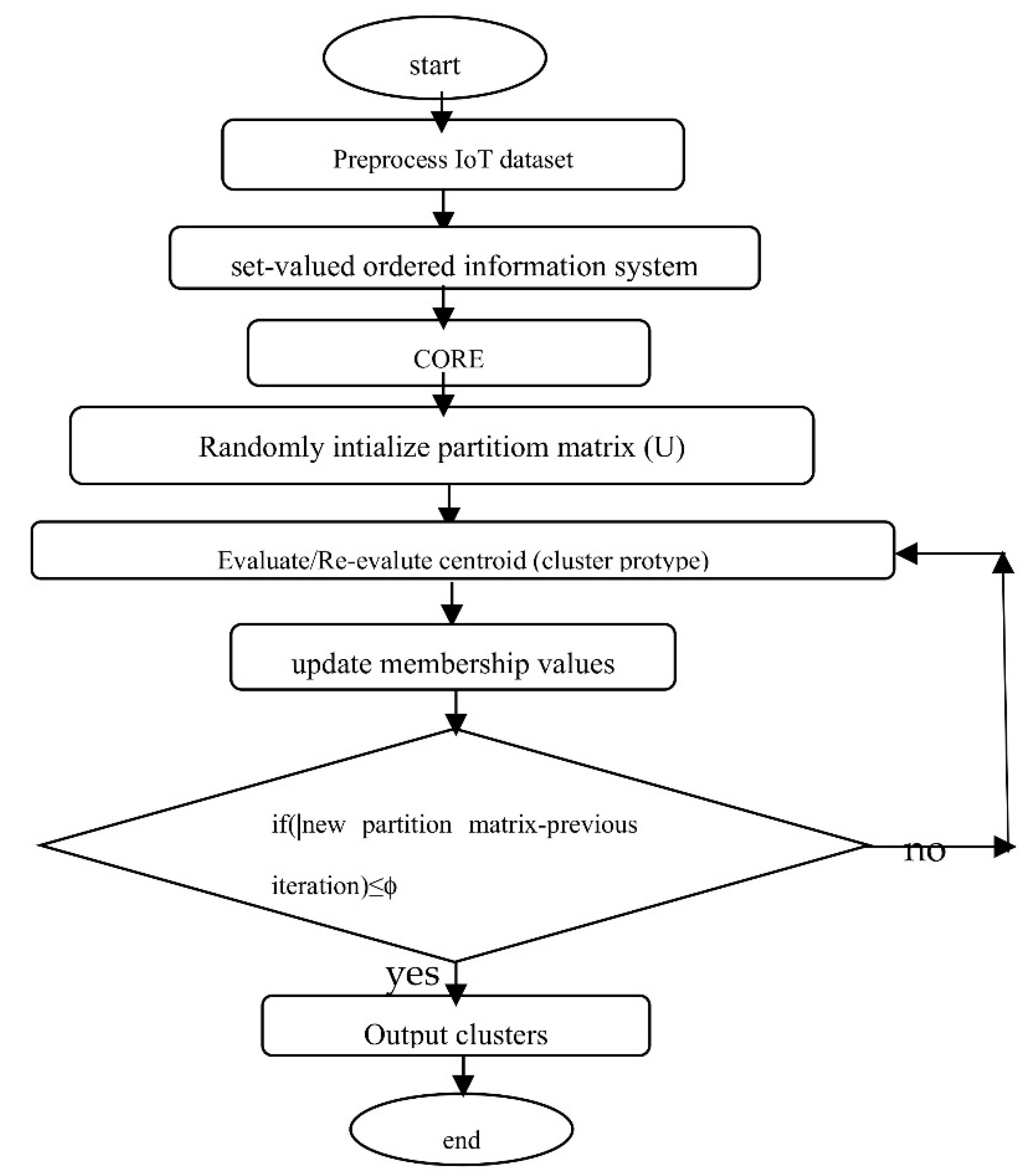
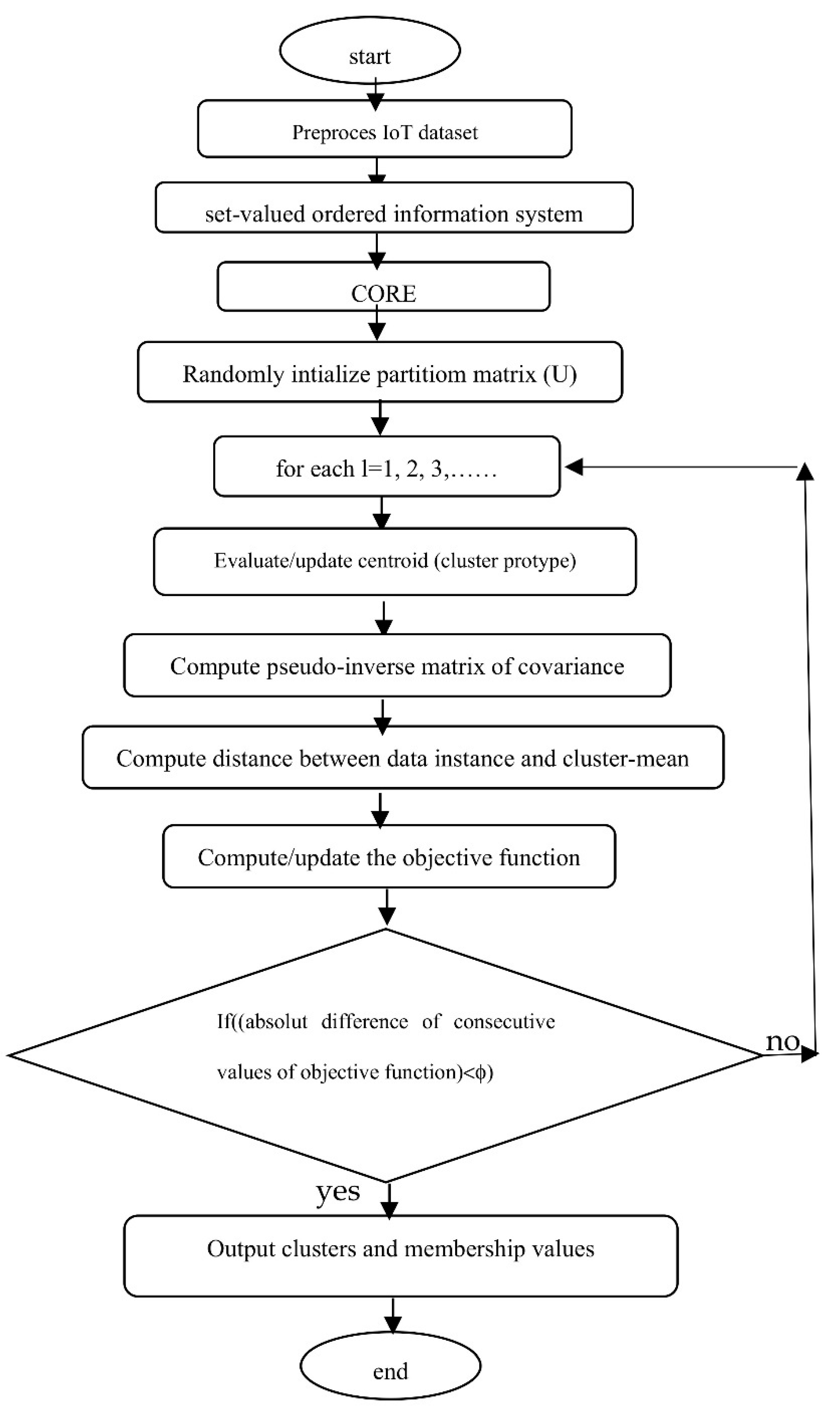
Here each cluster in the final output cluster set is a fuzzy set consisting of IoT data instances along with their membership grades. The IoT data instances which belong to all fuzzy clusters with minimum membership values would be treated as anomalies. A flowchart of the Nano topology-based fuzzy c-means clustering algorithm is given in Figure 1 below.

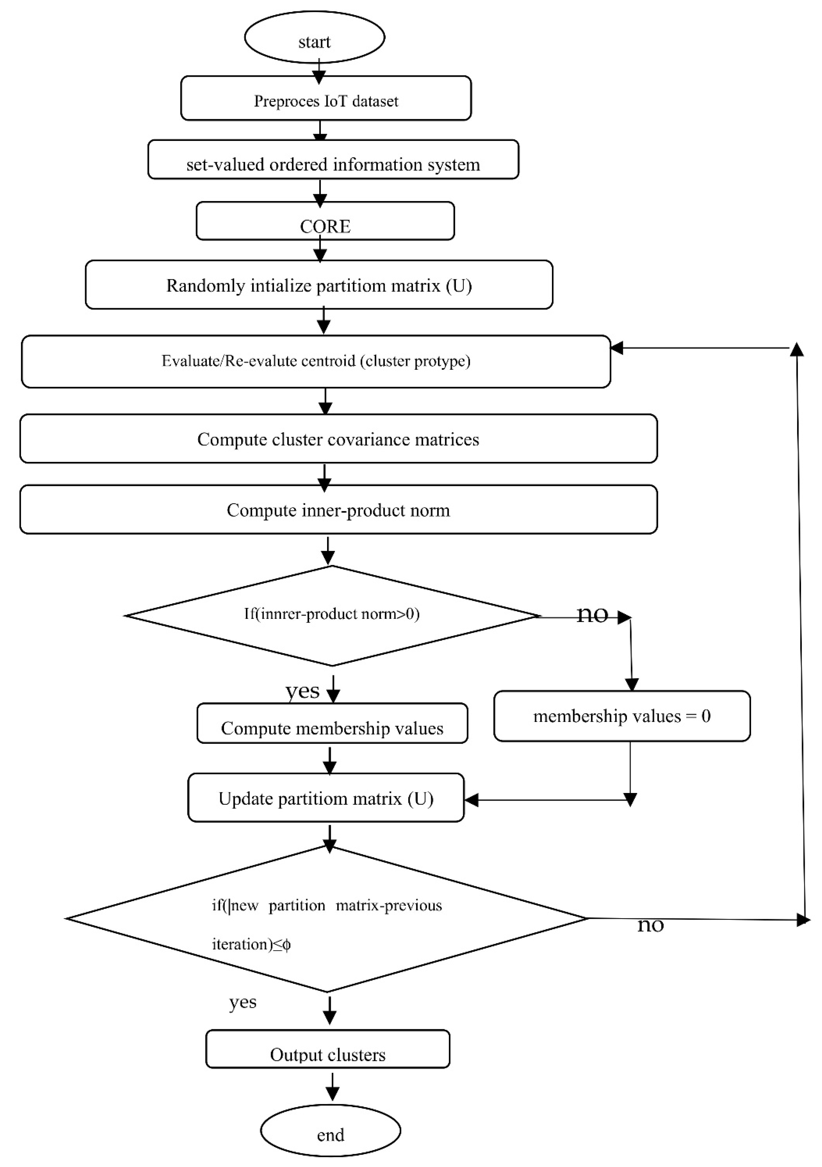
A flowchart of the Nano topology-based GK clustering algorithm is given in Figure 2 below.

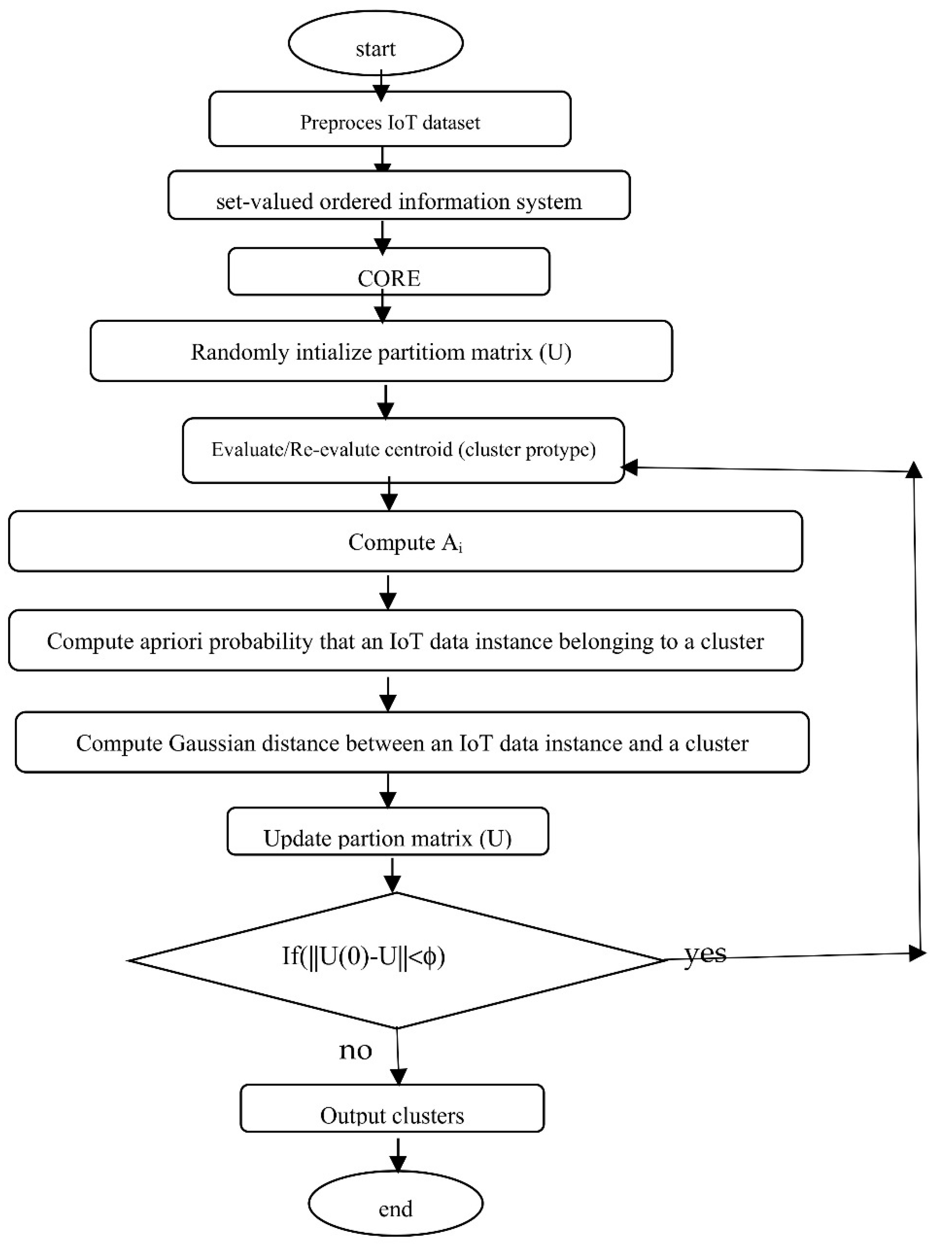
A flowchart of the Nano topology-based GG clustering algorithm is given in Figure 3 below.

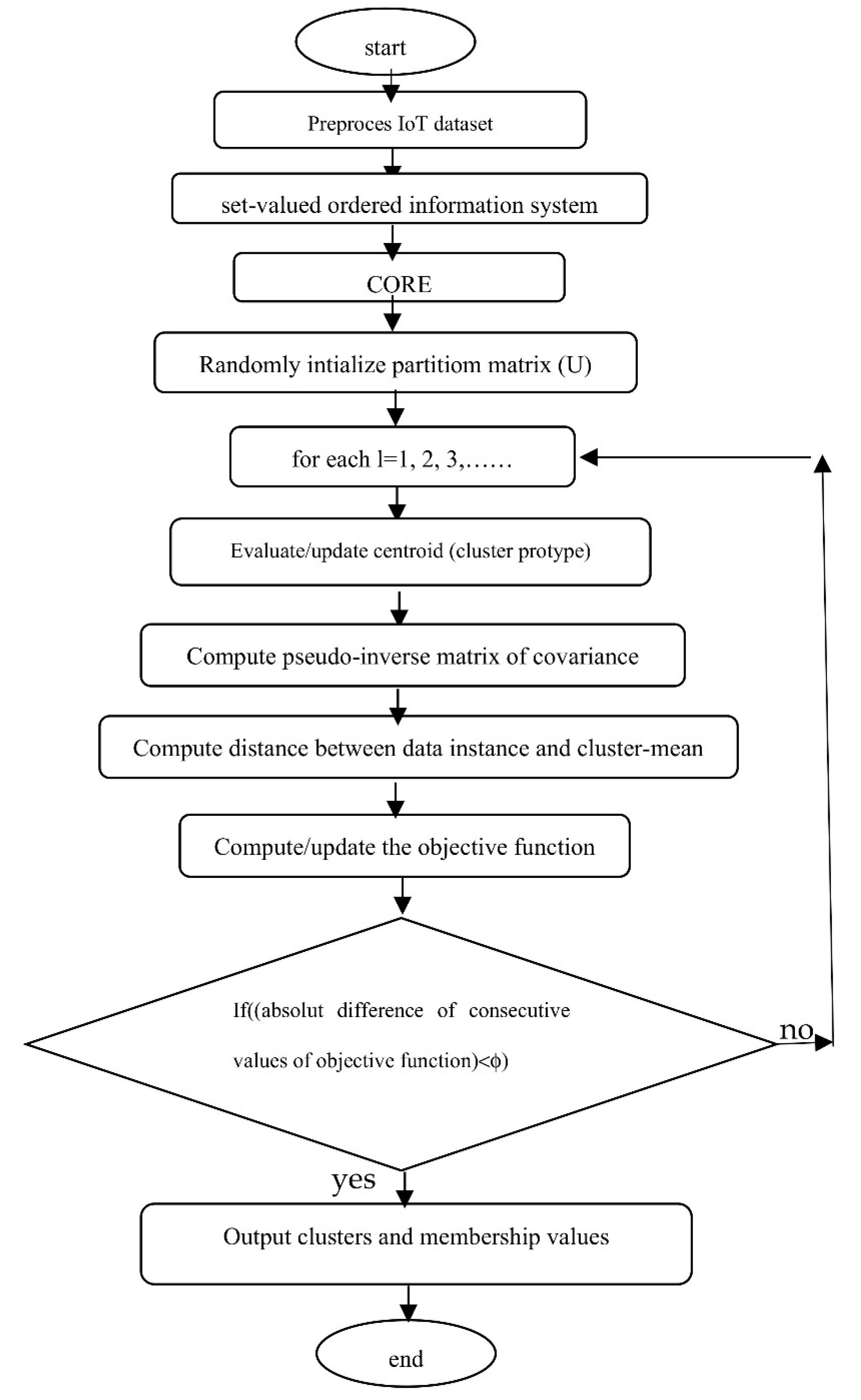
A flowchart of the Nano topology and Mahalanobis Distance based Fuzzy C-Means algorithm (NT-M-FCM) is given in Figure 4 below.

A flowchart of the Nano topology and Common Mahalanobis Distance based Fuzzy C-Means algorithm (NT-CM-FCM) is given in Figure 4 below.

The approaches employed here consist of various combinations of the algorithms of the form (Algorithm1 + Algorithm2), (Algorithm1 + Algorithm3), (Algorithm1 + Algorithm4), (Algorithm1 + Algorithm5), and (Algorithm1 + Algorithm6), where Algorthm1 (common to all) used for dimension reduction and others are used clustering. The approaches are well-described using flowcharts from Figure 1, Figure 2, Figure 3, Figure 4 and Figure 5. The methods supply specified number of fuzzy clusters in the lower-dimensional space. The anomalous items are those IoT data instances which either do not belong or belong to clusters with minimum membership values.

4. Complexity Analysis

If |U|=m, and |C|=n, the worst-case time-complexity algorithm1 is O(m².n). Since, FCM uses the norm inducing matrix, the time-complexity of distance function of fuzzy clusters is O(c.(c-1).d/2) = O(c².d). The worst-case complexity of FCM is O(m.c^2..d.i) = O(m.n.m^2.i) = O(m³.n.i), where d (≤ n) is the dimension of the subspace generated by Algorithm 1, c (≤ m) is the number of fuzzy clusters and I is the number of iterations. The overall time-complexity of NT-FCM is O(m².n + m³.d.i). Obviously, i ≤ m, and d≤n being small can be nexlected, therefore the overall worst-case time complexity of NT-FCM is O(m².n + m⁴), which shows that it is linear with respect to the dimension of the dataset. In general, n ≤ m, which gives worst-case complexity as O(m⁴).

In finding the compuational complexity of NT-GK Clustering algorithm, the complexity of NT is same as O(m².n). For finding new cluster, and fuzzy c-means membership, the algorithm needs O(c), and O(n.c), which are same as FCM. In this algorithm, the most important task is that each cluster has its own norm-inducing matrix, which produces inner product norm and the time-complexity of such for c clusters is O(k(m.d.m.d)) = O(m².d²), where k is the constant time required for computing A_i. If i be the number of iterations, the overall time-complexity is O(m².n + i.(c + n.c + c.m².d²)) = O(m².n + m².n + m⁴.d²)=O(m².n + m⁴.d²), where i=O(m), c=O(m) and d ≤ n ≤ m (in general) is small. Thus, the worst-case time-complexity of the algorithm is O(m⁴.d²).

The GG fuzzy clustering algorithm uses maximum likelyhood estimation measure which requires O(m.d). As it uses exponetial distance which introduces another level of complexity. The time complexity of NT-GG clustering algorithm is O(m².n + c.(m.c^..d².i) = O(m².n + m^4..d²), where i=O(m), c=O(m) and d ≤ n ≤ m (in general) is small. Thus, the worst-case time-complexity of the algorithm is O(m⁴.d²).

The M-FCM computes separate matrices for each cluster, so the time complexity of NT-M-FCM algorithm is O(m².n + i.(c + n.c + c.m.d²)) = O(m².n + m³.d²), where i=O(m), c=O(m) and d ≤ n ≤ m (in general) is small. Thus, the worst-case time-complexity of the algorithm is O(m³.d²).

Since CM-FCM uses a common covaricnace matrix instead of separate covarinace matrices of different custers, the time complexity of NT-CM-FCM algorithm is O(m².n + i.(c + n.c) + i.m.d²) = O O(m².n + m².d²), where i=O(m), c=O(m) and d ≤ n ≤ m (in general) is small. Thus the worst-case time-complexity of the algorithm is O(m³ + m².d²).

5. Experimental Analysis, Results and Discussions.

For testing the efficacy of the approaches employed here, two well-known datasets namely, KDDCup’99 Network Anomaly dataset [50] and Kitsune Network Attack dataset [51]. The datasets are obtained from UCI machine repository. The datasets allong with their characteristics in summarized form are described in Table1 below.

The experiments were conducted on a standard machine using two datasets described in Table 1. With KDDCup’99 [50], two datasets, one having different sizes but fixed dimensions and, other having fixed sizes and different dimensions are constructed. Similarly, with Kitsune dataset [51], two datasets of simlar sizes are constructed. The proposed methods namely NT-FCM, NT-GK, NT-GG, NT-M-FCM, and NT-CM-FCM are implemented using MATLAB with the aforesaid four datasets constructed from the aforesaid datasets. We also made comparative analysis of (FCM and NT-FCM), (GK and NT-GK), (GG and NT-GG), (M-FCM and NT-M-FCM), and (CM-FCN and NT-CM-FCM). Further, the performances all aforesaids methds along with FCM [41], GK [42], GG [43], M-FCM [47], and CM-FCM [47] are studied in manifolds, like accuracies in detection rates, the percentage of anomalies obtained, percentage of false alarm rates etc. The detailed findings of the aforesaid investigations are presented both in the tabular form and graphically in Table 2, Table 3 and Table 4 and graphically in Figure 6, Figure 7, Figure 8, Figure 9, Figure 10, Figure 11, Figure 12, Figure 13, Figure 14, Figure 15, Figure 16, Figure 17 and Figure 18 below.

The following inferences can be drawn from the obtained results. From Table 2, it is evident that that, out of all the traditional fuzzy clustering algorithm, the performannces in terms of the parameters like detection rate, accuracy rate, false alarm rate, denial of service, remote to local, user to root, and probe, of CM-FCM is quite better. However, its performance along with others reduces rapidly when a comparatively a larger dataset is considered which means that the performances depends both size and dimension of the dataset.

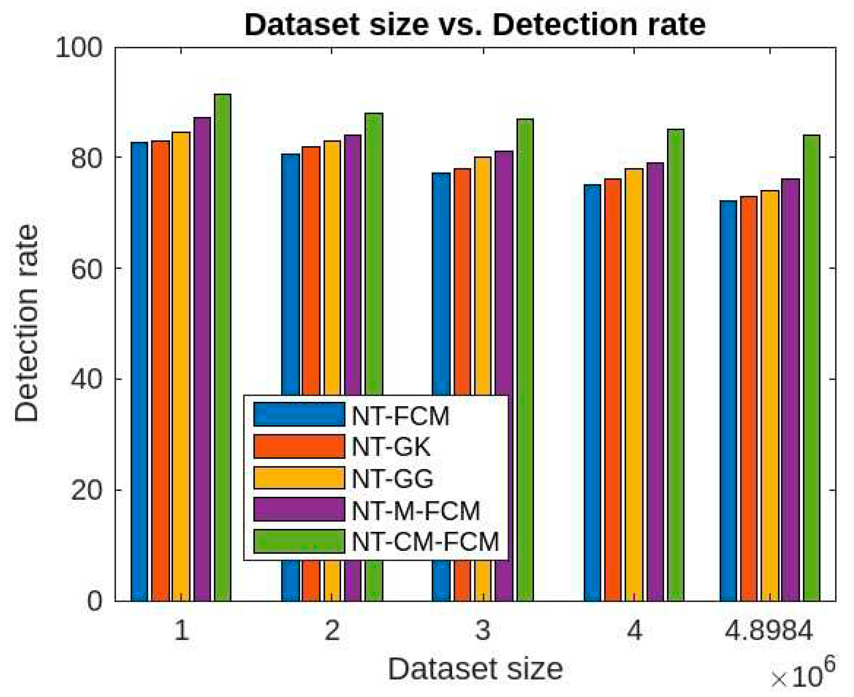
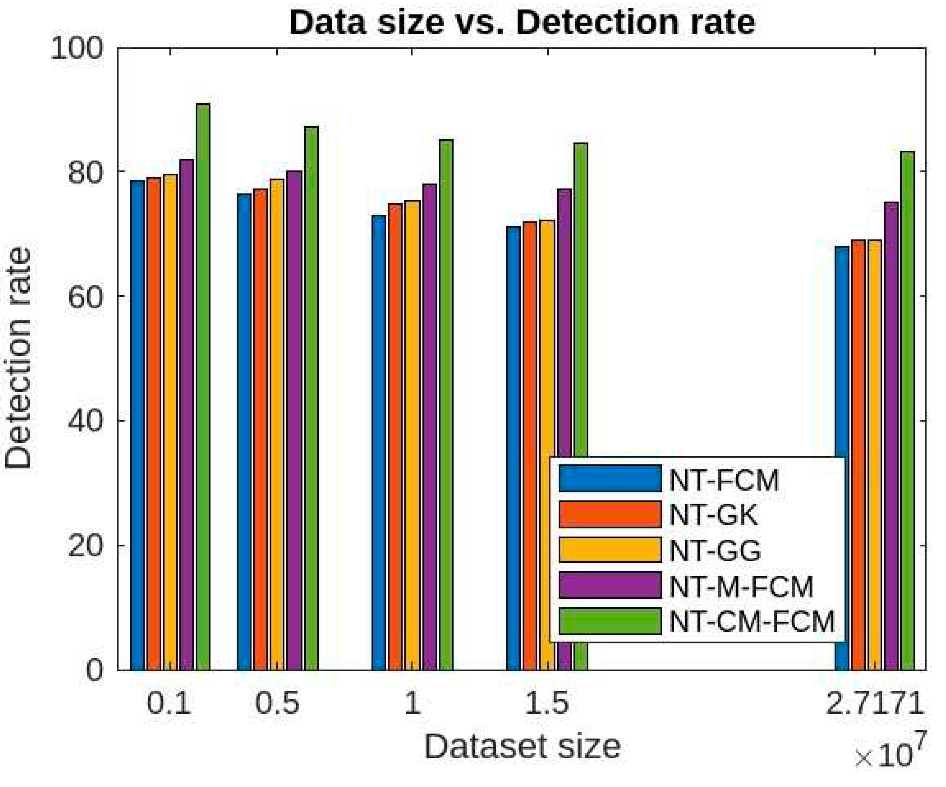
From Figure 6 and Figure 10, it can be concluded that the anomaly detection rates of all the algorithms improve if NT-based subspace clustering appraoch is considered. Though, the detection rate decreases with the increase of the size of the dataset, but the rate of decrease is much slow. Among all the NT-based approach, NT-CM-FCM is found to be comparatively as it’s anomaly detection rate ranges from 84.02% to 91.3% for the KDDCup’99 dataset and 83.21% to 90.8% for the dataset Kitsune.

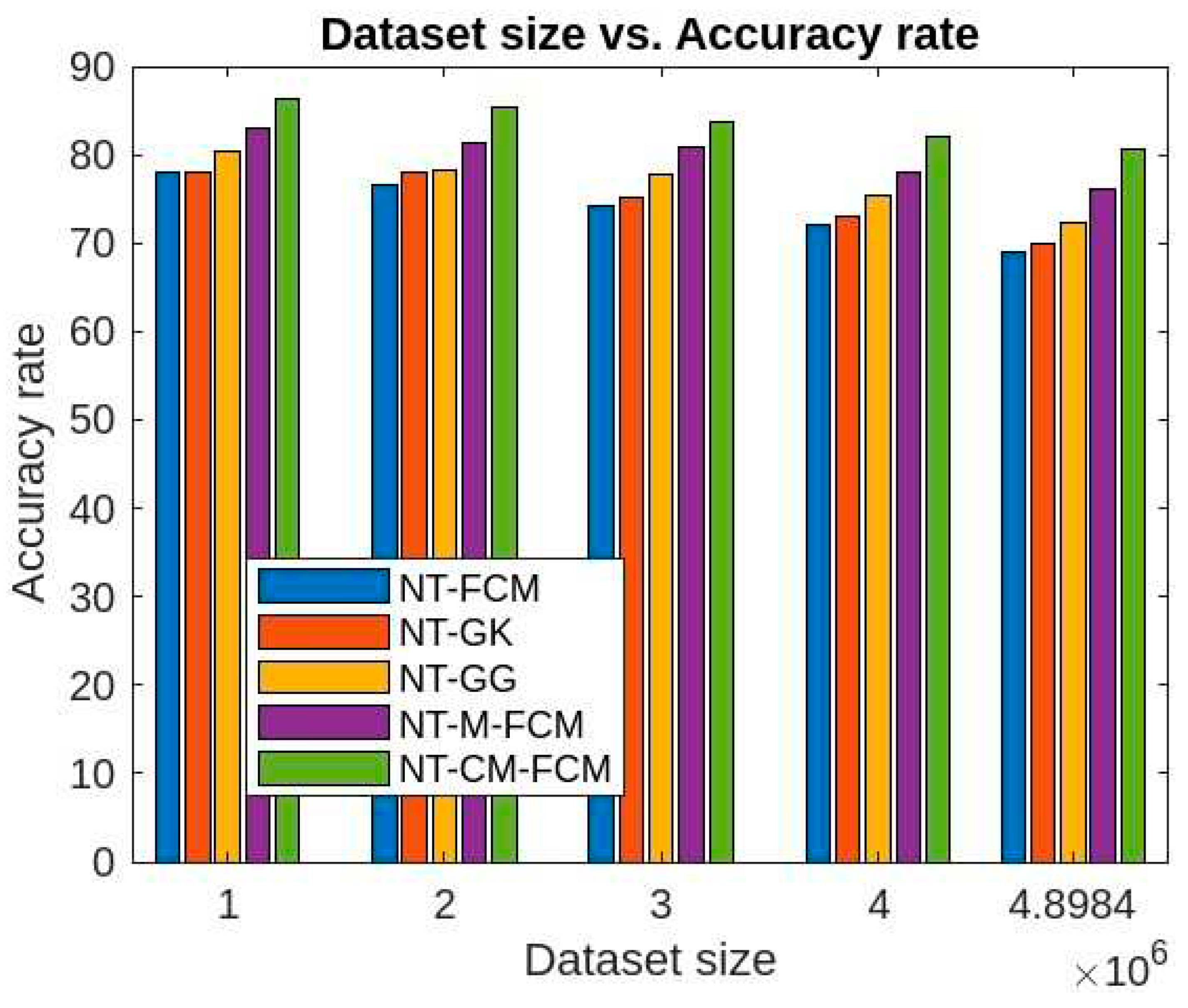
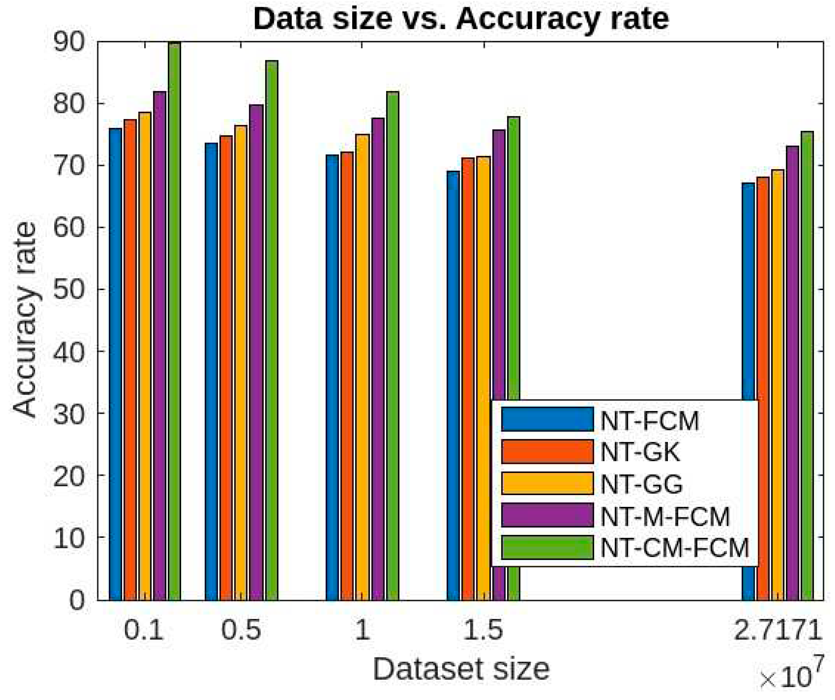
As per as accuracy of anomaly detection is concern, Figure 7 and Figure 11 show that NT-based approach of the fuzzy clustering algorithms perform implressively in comparison to the traditional fuzzy clustering approaches. Similar to the detection rate, the accuarcy rate decrement with respect to the increament of dataset size is visibly less. The NT-CM—FCM is found to be comaratively better as its accuracy of anomaly detection ranges from 80.54% to 86.5% for KDDCup’99 dataset and from 75.37% to 82.6% for the Kitsune dataset.

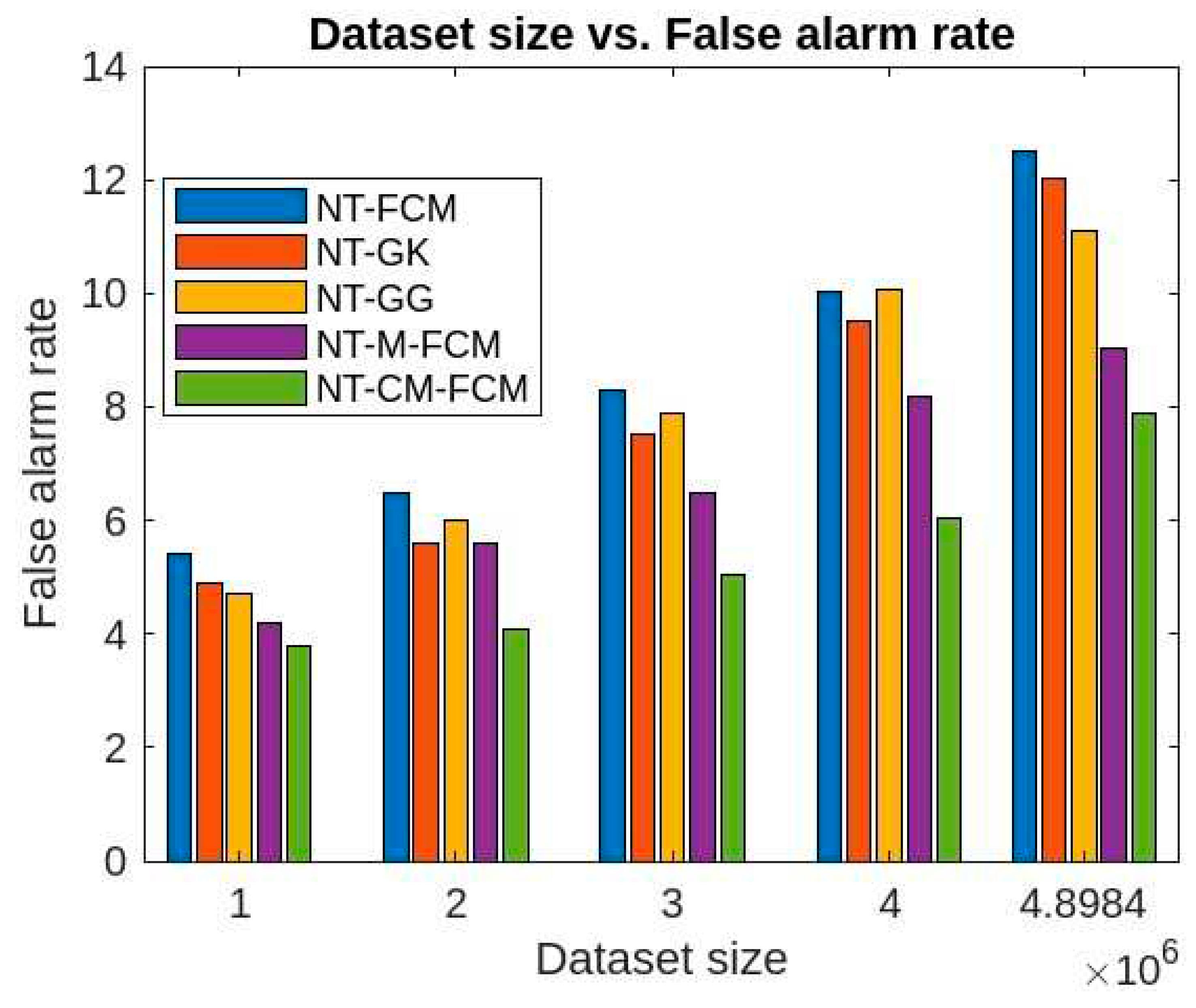
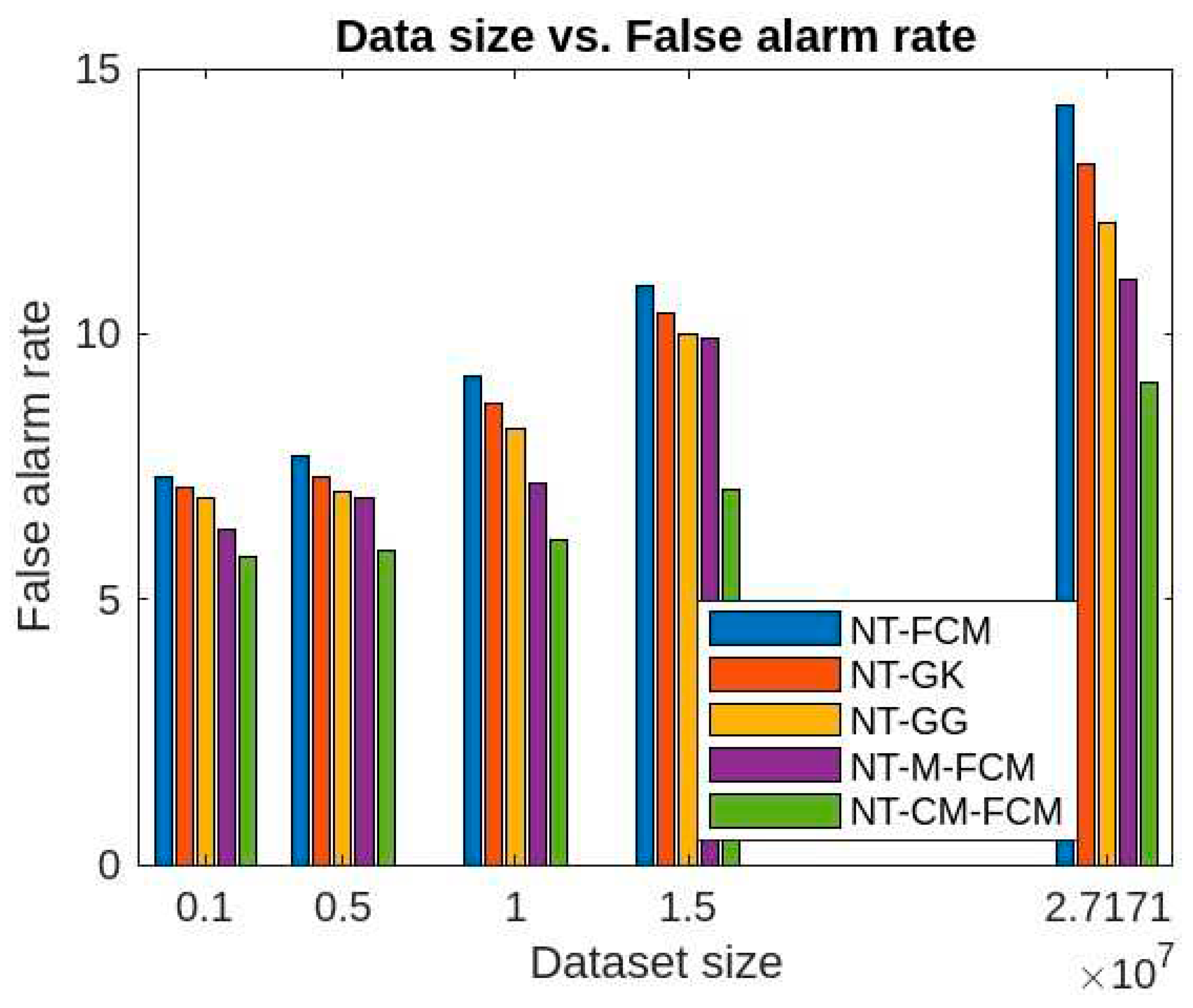
From Figure 8 and Figure 11, it is evident that the false alarm rates of NT-based algorithms are quite lesser than the traditional fuzzy clustering algorithms and also the performance of NT-CM-FCM is comparatively much better than others. The false alarm rate for KDDCup’99 is 3.78-7.89% and for Kitsune dataset is 5.8-9.09% for different sizes of the two datasets.

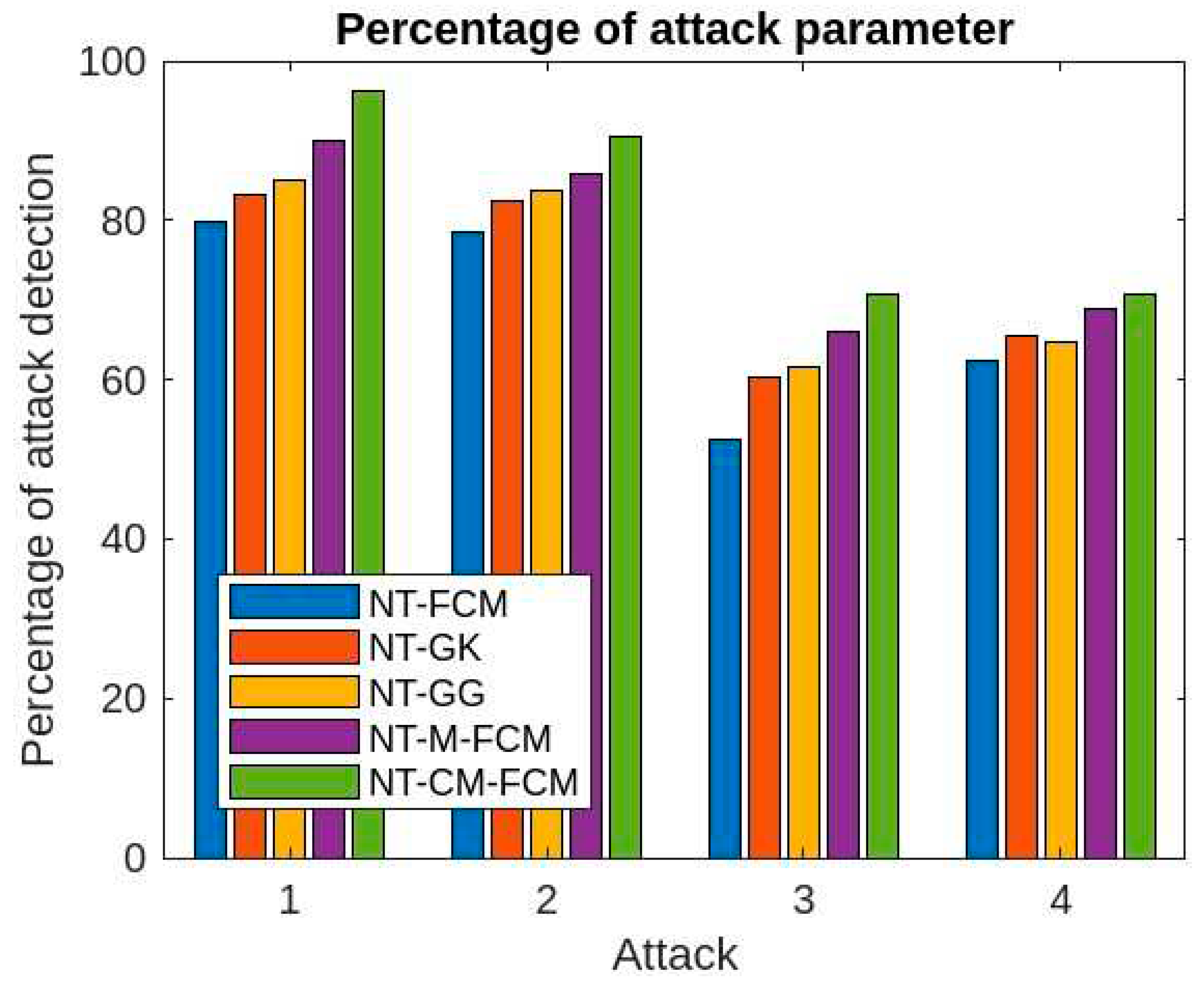
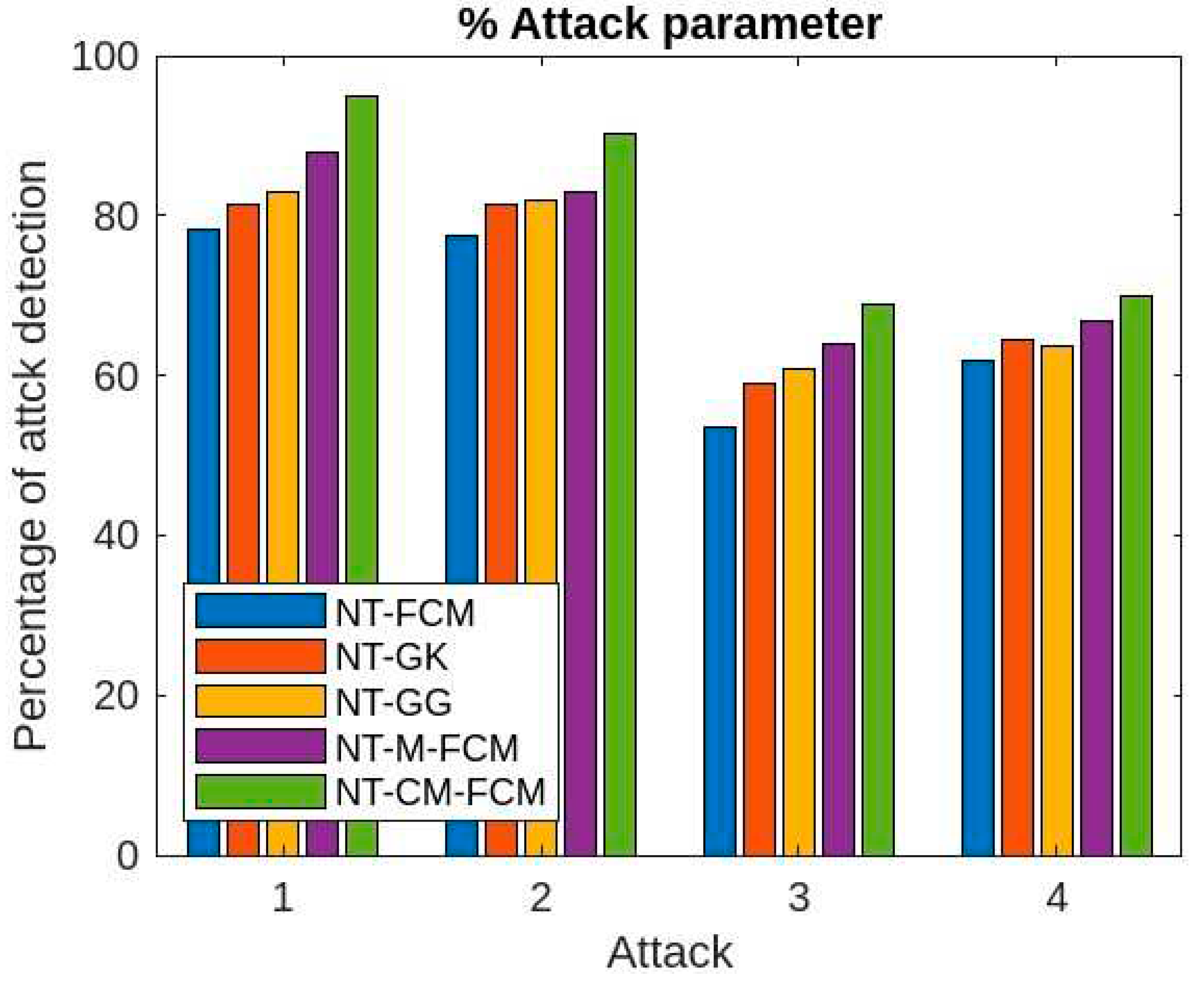
It is evident from the Table 2, Table 3 and Table 4, and Figure 9 and Figure 12, the performances of NT-based algorithms with respect to different attack parameters (denial of service, remote to local, user to root and probe) are comparative better than the traditional algorithms. Here also, the NT-CM-FCM algorithm outperforms others.

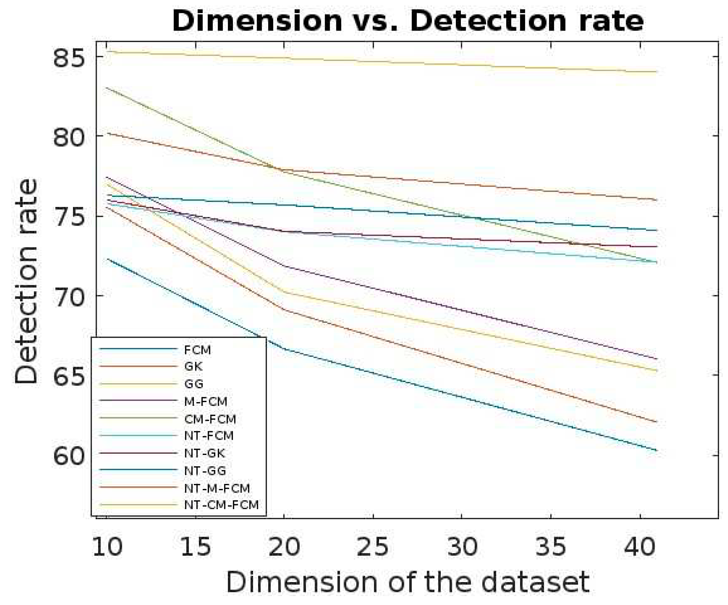
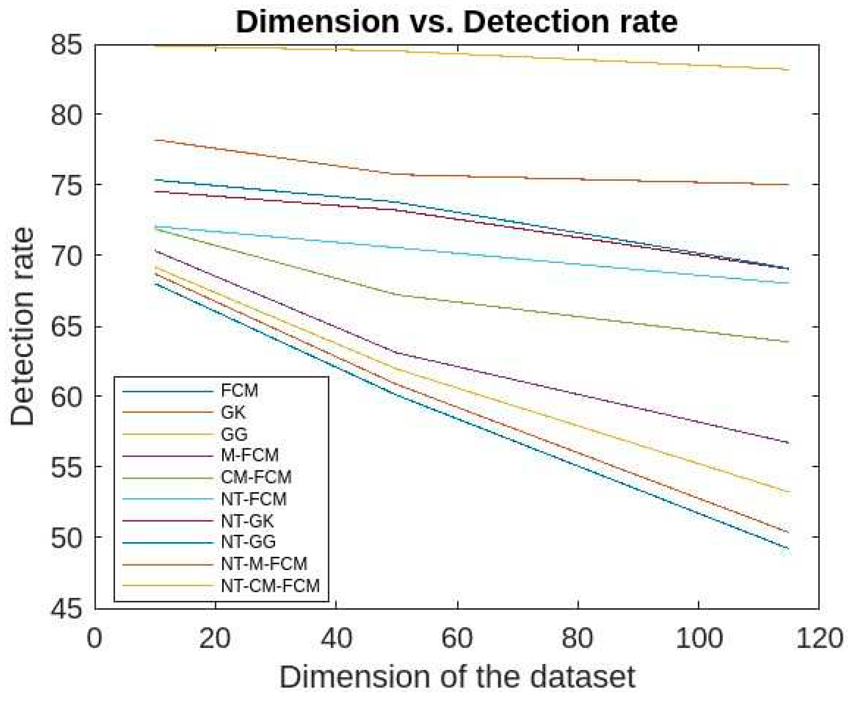
From Figure 13 and Figure 14, it can be inferred that for different sizes of the dimensions of the KDDCup’99, the detection rate ranges of FCM, GK, GG, M-FCM, CM-FCM, NT-FCM, NT-GK, NT-GG, NT-M-FCM, and NT-CM-FCM are respectively as 60.3 - 72.34, 62.06 – 75.56, 65.3 – 77.01, 66.03 – 77.45, 72.08 – 83.05, 72.1 – 75.78, 73.05 – 76.01, 74.1 – 76.3, 76.02 – 80.2, and 84.02 – 85.3 and for the Kitsune dataset the same are as 49.21 - 68.03, 50.36 - 68.72, 53.23 - 69.19, 56.73 - 70.36, 63.88 - 71.9, 68.03 - 72.09, 69.05 - 74.56, 69.1 - 75.37, 75.04 - 78.23, 83.21 - 84.89. It can be inferred from the data that for lower dimensional dataset, most of the algorithms work nicely, even CM-FCM’s efficacy of anomaly detection is higher than some of the NT-based appraoches. However, when the dimension increases, the efficacies of all the traditional fuzzy clustering algorithms fall rapidly. The NT-based algorithms perform better comparatively, which show that NT-based algorithms are less dependant on the dimension of the datasets. It is to be mention that algorithm NT-M-FCM, and NT-CM-FCM’s anomaly detection rates are much better than the others.

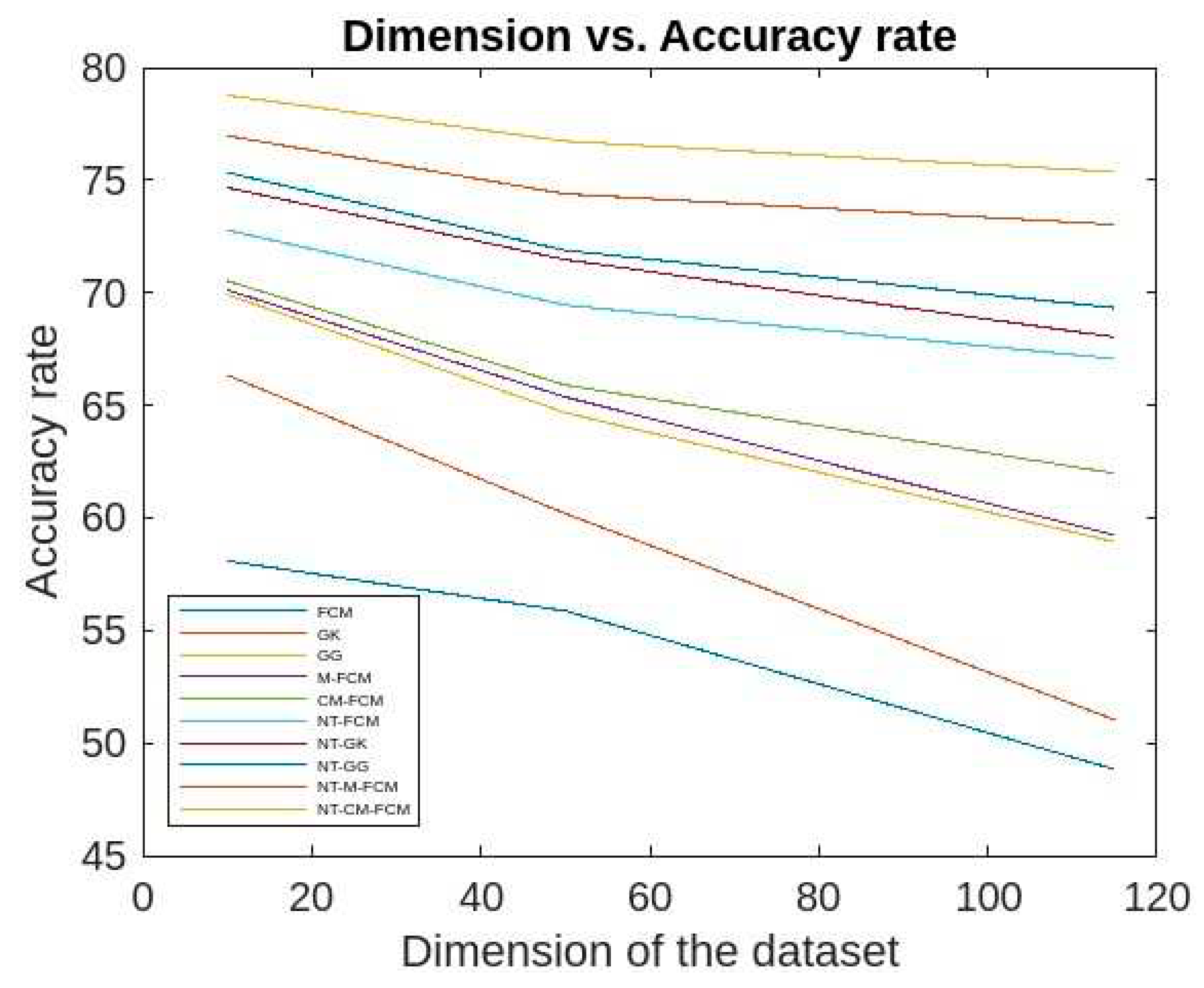
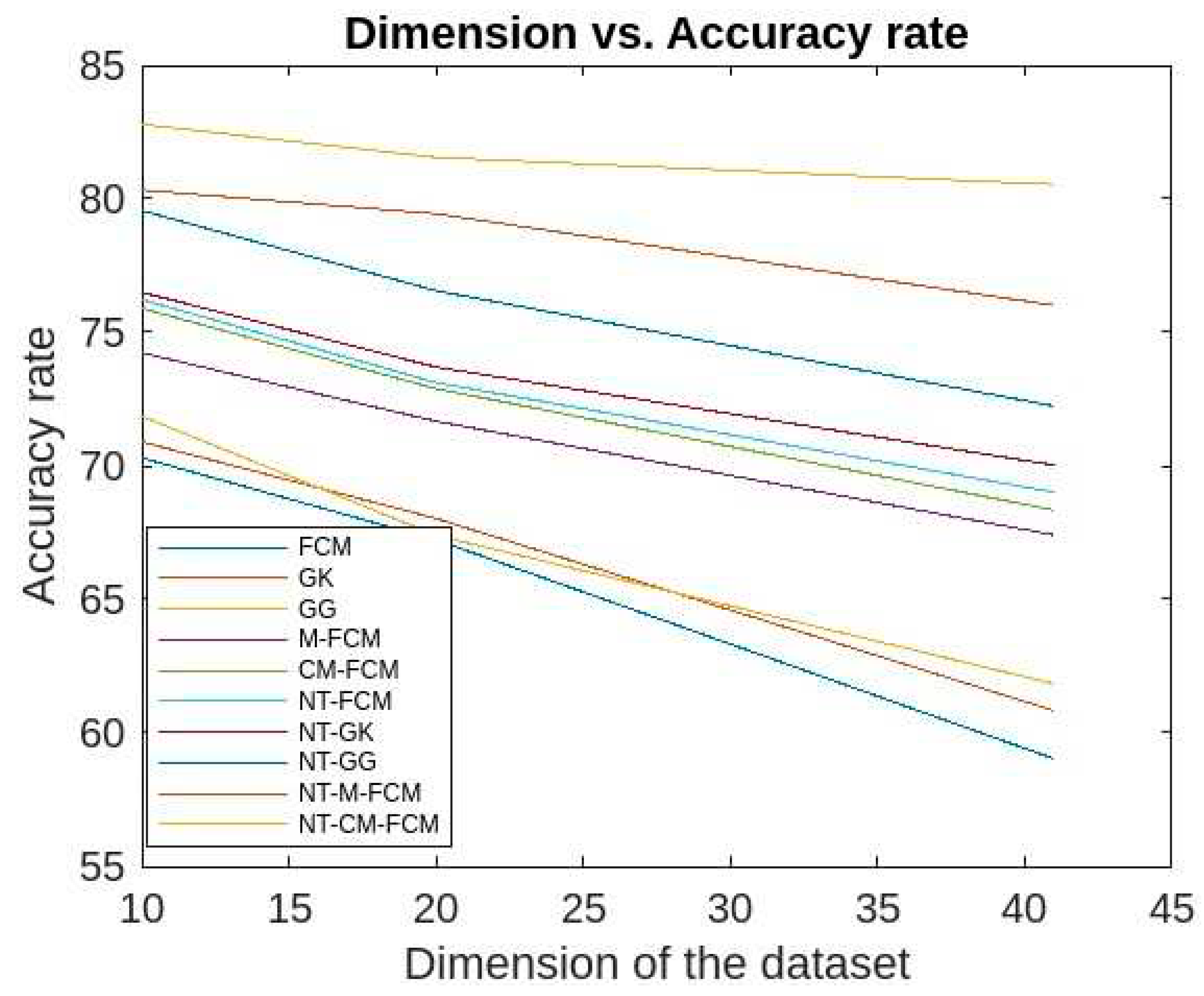
Figure 15 and Figure 16 give the accuracy rates of detection for all the foresaid ten algorithms are respectively as 59.03 - 70.3, 60.83 - 70.9, 61.84 - 71.86, 67.41 - 74.23, 68.34 - 75.9, 69.01 - 76.23, 70.03 - 76.5, 72.24 - 79.56, 76.01 - 80.33, and 80.54 - 82.79 for the data KDDCup’99 and 48.83 - 58.09, 51.03 - 66.34, 58.94 - 69.92, 59.23 - 70.12, 61.98 - 70.53, 67.07 - 72.78, 68.03 - 74.67, 69.33 - 75.34, 73.03 - 76.97, and 75.37 - 78.77 for the dataset Kitsune. Since the accuracy ranges are more for the traditional fuzzy clustering algorithms than the NT-based algorithms, which in turn eastablished the fact that later algorithms are less dependent on the sizes of dimensions of the datasets. It is to be mentioned here that, NT-CM-FCM is comparatively better than others in terms of accuracy rate of anomaly detection.

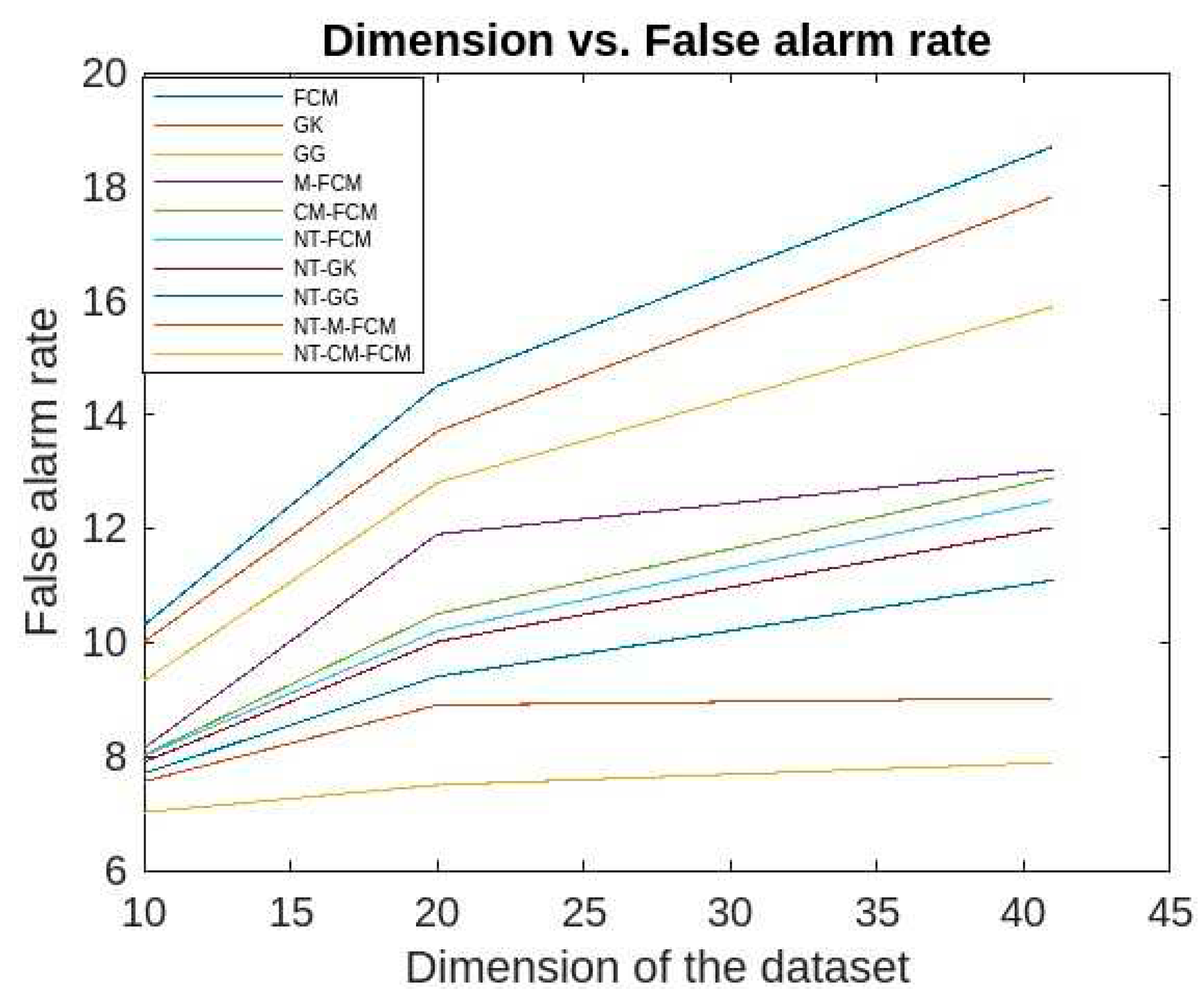
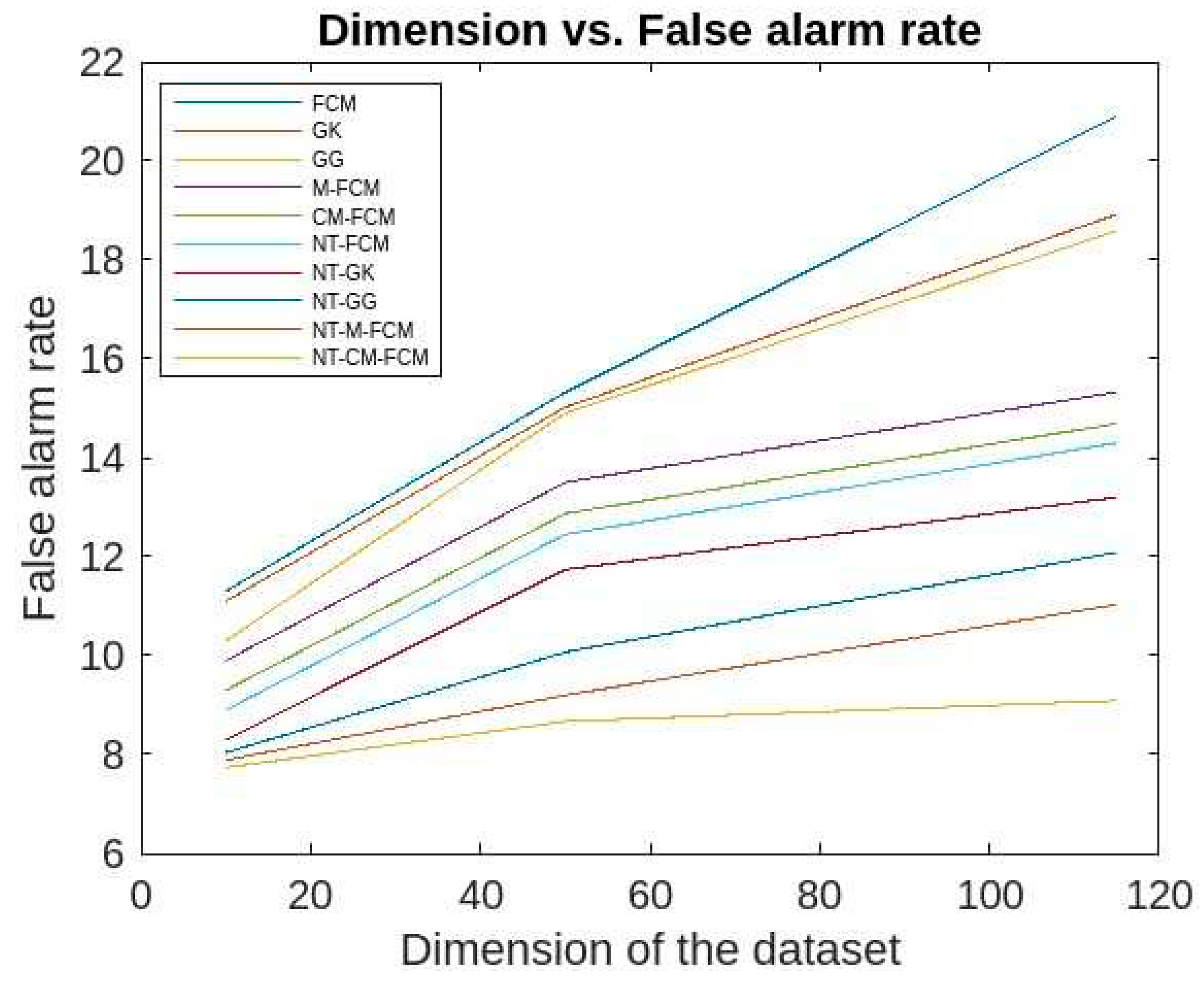
The false alarm rates of the aforesaid algorithms for the KDDCup’99 data are respective ranges 10.3-18.7, 10.01-17.82, 9.32-15.89, 8.14-13.03, 8.02-12.89, 8.01-12.5, 7.9-12.02, 7.7-11.09, 7.56-9.02, 7.02-7.89 and for Kitsune dataset are respective ranges 20.9-11.3, 18.92-11.1, 18.59-10.3, 15.33-9.9, 14.69-9.3, 14.3-8.9, 13.2- 8.3, 12.09-8.04, 11.03-7.89, 9.09-7.74 which is evident from Figure 17 and 18. It has been observed that the false alarm rates of all the algorithm increases with the increase in the dimension of datasets. However, for the NT-based algorithms the rate of increase is comparatively slower and NT-CM-FCM it is slowest. It is also observed the rates of decreases from left right which shows that NT-CM-FCM is best among all the algorithms whether traditional or NT-based.

6. Conclusions, Limitations and Lines for Future Works

6.1. Conclusions

In this article, two-phased methods of fuzzy subspace clustering for anomaly detections were proposed. The input dataset is initially transformed into a set-valued information system using the approach which establishes a dominance relation on it. Then a nano topology along with its basis is constructed by removing insignificant attributes of the dataset by the dominance relation. The constructed nano topology creates a lower-dimensional space of the original dataset. In the second phase, fuzzy clustering algorithms were employed for anomaly detections. For fuzzy clustering, the algorithms namely FCM [41], GK [42,47], GG [43,47], M-FCM [47], and CM-FCM [47] were used. We named the proposed algorithms as NT-FCM, NT-GK, NT-GG, NT-M-FCM, and NT-CM-FCM. Each of the proposed method supplies a set of fuzzy clusters. The data instance not belonging any cluster or belonging any cluster with minimum membership value can be treated as anomaly. The efficacies of the proposed approaches were studied by experimental analysis on a synthetic dataset KDDCup’99 [50] and a real-life dataset Kitsune [51] and comparative studies have made with traditional fuzzy clustering approaches. The results showed that the NT-based algorithms outperform the traditional approaches in terms of anomaly detection rates, accuracy rates, false alarm rates and run-time complexities.

Though among all the aforesaid methods, NT-CM-FCM is the best, its traditional algorithm CM-FCM sometimes performs better than other NT-based fuzzy clustering approaches.

Finally, any NT-based method is a combination two algorithms. The algorithm1 is the nano topology based algorithm which returns subspaces of the datasets and which are the input to the fuzzy clustering algorithms. The run-time complexity of algorithm1 depends on the data size and dimensions. It is quadratic to the dataset sizes and linear to the dimension of the dataset. Since size of any dataset is quite bigger than its dimension size, and the dimension size of subspace is quite small, the time complexity of all the aforesaid NT-based algorithms depend on time complexity of algorithm1 and the dataset size. It is to mentioned that the NT-M-FCM, and NT-CM-FCM run in cubic time, but others run in biquadratic time.

6.2. Limitations and Lines for Future Works

Though the NT-based approaches are performing better than the traditional fuzzy clustering approaches, they are not free from limitations. Firstly, though using algorithm1, the computational cost of any NT-based algorithm can be reduced upto some extent, still they are expensive that non-fuzzy clustering, as they require optimization over multiple membership grades. Secondly, choosing the number of clusters and membership function is the most challenging task which requires either trial/error approach or domain expert.

The future lines of work can be focused towards the following.

In the future, the time attribute can be addressed separately to find fuzzy clusters along with lifetimes which may provide detailed insight of the IoT system.
In the future, detecting anomalies from high-dimensional data may be accomplished with an effective supervised approach.

References

Sethi, P., and Sarangi, S. Internet of things: Architectures, protocols, and applications, Journal of Electrical and Computer Engineering, pp. 1–25,2017. [CrossRef]
The, H. Y., Wang, K. I., and Kempa-Liehr, A. W. Expect the unexpected: Un-supervised feature selection for automated sensor anomaly detection, IEEE Sensors Journal, pp. 18033 – 18046, 2021. [CrossRef]
Erfani S. M., Rajasegarar S., Karunasekera S., Leckie, C. High-dimensional and large-scale anomaly detection using a linear one-class SVM with deep learning, Pattern Recogn, Vol. 58, pp.121–134, 2016.
Hodge, V., Austin, J. A survey of outlier detection methodologies, Artif Intell Rev, Vol..22(2), pp. 85–126, 2004.
Hartigan, J. A. Clustering Algorithms, John Wiley & Sons, 1975.
Aggarwal C. C., and Philip, S. Y. An effective and efficient algorithm for high-dimensional outlier detection, VLDB J. Vol. 14(2), pp. 211–221, 2005.
Ramchandran, A., Sangaiah, A. K. Chapter 11 - Unsupervised Anomaly Detection for High Dimensional Data—an Exploratory Analysis, Computational Intelligence for Multimedia Big Data on the Cloud with Engineering Applications, Intelligent Data-Centric Systems, pp. 233-251, 2018.
Pawlak, Z., Rough sets, International Journal of Computer and Information Sciences, Vol. 11, pp. 341–356, 1982.
Mazarbhuiya, F. A. Detecting Anomaly using Neighborhood Rough Set based Classification Approach, ICIC Express Letters, Vol. 17(1), pp. 73-80, 2023.
Thivagar, M. L., Richard, C. On nano forms of weakly open sets, International Journal of Mathematics and Statistics Invention. 1(1), pp. 31–37, 2013.
Thivagar, M. L. and Priyalatha, S.P.R. Medical diagnosis in an indiscernibility matrix based on nano topology, Cogent Mathematics, 4: 1330180, pp. 1-9, 2017. [CrossRef]
Mung, G., Li, S., and Carle, G. Traffic Anomaly Detection Using k-Means Clustering, Allen institute for Artificial Intelligence, 2007.
Ren, W., Cao, J., and Wu, X. Application of network intrusion detection based on fuzzy c-means clustering algorithm, The 3rd International Symposium on Intelligent Information Technology Application, pp.19-22, 2009.
Mazarbhuiya, F. A. AlZahrani, M. Y., and Georgieva, L. Anomaly detection using agglomerative hierarchical clustering algorithm, Lecture Notes in Electrical Engineering, Singapore, Springer, 2018. [CrossRef]
Mazarbhuiya, F. A. AlZahrani, M. Y., and A. K. Mahanta, Detecting Anomaly Using Partitioning Clustering with Merging; ICIC Express Letters Vol. 14(10), Japan, pp. 951-960, 2020.
Retting, L.; Khayati, M.; Cudre-Mauroux, P.; Piorkowski, M. Online anomaly detection over Big Data streams. In Proceedings of the 2015 IEEE International Conference on Big Data, Santa Clara, CA, USA, 29 October–1 November 2015.
Alguliyev, R.; Aliguliyev, R.; Sukhostat, L. Anomaly Detection in Big Data based on Clustering. Stat. Optim. Inf. Comput. 2017, 5, 325–340. [CrossRef]
Hahsler, M.; Piekenbrock, M.; Doran, D. dbscan: Fast Density-based clustering with R. J. Stat. Softw. 2019, 91, 1–30. [CrossRef]
Song, H.; Jiang, Z.; Men, A.; Yang, B. A Hybrid Semi-Supervised Anomaly Detection Model for High Dimensional data. Comput. Intell. Neurosci. 2017, 2017, 1–9. [CrossRef]
Mazarbhuiya, F. A. Detecting IoT Anomaly Using Rough Set and Density Based Subspace Clustering, ICIC Express Letters (accepted to be published shortly).
Alghawli, A.S. Complex methods detect anomalies in real time based on time series analysis. Alex. Eng. J. 2022, 61, 549–561. [CrossRef]
Younas, M.Z. Anomaly Detection using Data Mining Techniques: A Review. Int. J. Res. Appl. Sci. Eng. Technol. 2020, 8, 568–574. [CrossRef]
Thudumu, S.; Branch, P.; Jin, J.; Singh, J. A comprehensive survey of anomaly detection techniques for high dimensional big data. J. Big Data 2020, 7, 42. [CrossRef]
Habeeb, R.A.A.; Nasauddin, F.; Gani, A.; Hashem, I.A.T.; Ahmed, E.; Imran, M. Real-time big data processing for anomaly detection: A Survey. Int. J. Inf. Manag. 2019, 45, 289–307. [CrossRef]
Wang, B.; Hua, Q.; Zhang, H.; Tan, X.; Nan, Y.; Chen, R.; Shu, X. Research on anomaly detection and real-time reliability evaluation with the log of cloud platform. Alex. Eng. J. 2022, 61, 7183–7193. [CrossRef]
Halstead, B.; Koh, Y.S.; Riddle, P.; Pechenizkiy, M.; Bifet, A. Combining Diverse Meta-Features to Accurately Identify Recurring Concept Drit in Data Streams. ACM Trans. Knowl. Discov. Data 2023. [CrossRef]
Zhao, Z.; Birke, R.; Han, R.; Robu, B.; Bouchenak, S.; Ben Mokhtar, S.; Chen, L.Y. RAD: On-line Anomaly Detection for Highly Unreliable Data. arXiv 2019, arXiv:1911.04383. https://arxiv.org/abs/1911.04383.
Chenaghlou, M.; Moshtaghi, M.; Lekhie, C.; Salahi, M. Online Clustering for Evolving Data Streams with Online Anomaly Detection. Advances in Knowledge Discovery and Data Mining. In Proceedings of the 22nd Pacific-Asia Conference, PAKDD 2018, Melbourne, VIC, Australia, 3–6 June 2018; pp. 508–521.
Firoozjaei, M.D.; Mahmoudyar, N.; Baseri, Y.; Ghorbani, A.A. An evaluation framework for industrial control system cyber incidents. Int. J. Crit. Infrastruct. Prot. 2022, 36, 100487. [CrossRef]
Chen, Q.; Zhou, M.; Cai, Z.; Su, S. Compliance Checking Based Detection of Insider Threat in Industrial Control System of Power Utilities. In Proceedings of the 2022 7th Asia Conference on Power and Electrical Engineering (ACPEE), Hangzhou, China, 15–17, April 2022; pp. 1142–1147.
Zhao, Z.; Mehrotra, K.G.;Mohan, C.K. Online Anomaly Detection Using Random Forest. In Recent Trends and Future Technology in Applied Intelligence; Mouhoub, M., Sadaoui, S., Ait Mohamed, O., Ali, M., Eds.; IEA/AIE 2018; Lecture Notes in Computer Science; Springer: Cham, Switzerland.
Izakian, H.; Pedrycz, W. Anomaly detection in time series data using fuzzy c-means clustering. In Proceedings of the 2013 Joint IFSA World congress and NAFIPS Annual meeting, Edmonton, AB, Canada, 24–28 June 2013.
Decker, L.; Leite, D.; Giommi, L.; Bonakorsi, D. Real-time anomaly detection in data centers for log-based predictive maintenance using fuzzy-rule based approach. arXiv 2020, arXiv:2004.13527v1. https://arxiv.org/pdf/2004.13527.pdf.
Masdari, M.; Khezri, H. Towards fuzzy anomaly detection-based security: A comprehensive review. Fuzzy Optim. Decis. Mak. 2020, 20, 1–49. [CrossRef]
de Campos Souza, P.V.; Guimarães, A.J.; Rezende, T.S.; Silva Araujo, V.J.; Araujo, V.S. Detection of Anomalies in Large-Scale Cyberattacks Using Fuzzy Neural Networks. AI 2020, 1, 92–116. https://www.mdpi.com/2673-2688/1/1/5. [CrossRef]
P. D. Talagala, Rob J. Hyndman, and Kate Smith-Miles, Anomaly Detection in High-Dimensional Data, Journal of Computational and Graphical Statistics, Vol. 30(2), 2021, pp. 360-374.
Mustafa Al Samara, Ismail Bennis, Abdelhafid Abouaissa and Pascal Lorenz, A Survey of Outlier Detection Techniques in IoT: Review and Classification, Journal of Sensor and Actuator Networks, Vol 11(4), 2022, pp. 1-31. [CrossRef]
Yugandhar, A. Sashirekha , S. K, Dimensional Reduction of Data for Anomaly Detection and Speed Performance using PCA and DBSCAN, International Journal of Engineering and Advanced Technology, Vol. 9(1S2), 2019, pp. 39-41.
Mazarbhuiya, F. A.; Shenify, M.; A Mixed Clustering Approach for Real-Time Anomaly Detection, Appl. Sci. 2023, 13, 4151. [CrossRef]
Mazarbhuiya, F. A. and Shenify, M; Real-time Anomaly Detection with Subspace Periodic Clustering Approach, Applied Science, MDPI, Vol. 13(13), 2023, Switzerland, pp. 1-21.
Harish, B. S.; and Kumar, S. V. A. Anomaly based Intrusion Detection using Modified Fuzzy Clustering, International Journal of Interactive Multimedia and Artificial Intelligence, Vol. 4(6), 2017, pp. 54-59. [CrossRef]
Gustafson, D. E. & Kessel, W., Fuzzy clustering with a fuzzy covariance matrix. In Proc. of IEEE Conf. on Decision and Control including the 17th Symposium on Adaptive Processes, San Diego, 1979, pp. 761-766. [CrossRef]
Haldar, N. A. H.; Khan, F. A.; Ali, A.; and Abbas, H., Arrhythmia classification using Mahalanobis distance-based improved Fuzzy C-Means clustering for mobile health monitoring systems, Neurocomputing, vol.220 (12), pp. 221–235, 2017. [CrossRef]
Zhao, X. M.; Li, Y.; and Zhao, Q. H., Mahalanobis distance based on fuzzy clustering algorithm for image segmentation, Digital Signal Processing, vol. 43 (12), pp. 8–16, 2015. [CrossRef]
Ghorbani, H., Mahalanobis Distance and Its Application for Detecting Multivariate Outliers, FACTA UNIVERSITATIS (NIS) Ser. Math. Inform. Vol. 34(3), 2019, pp. 583–595. [CrossRef]
Mahalanobis, P. C., On the generalized distance in statistics. Proceedings of the National Institute of Sciences (Calcutta), 1936, 2, pp. 49–55.
Yih, J-M; and Lin, Y-H., Normalized clustering algorithm based on Mahalanobis distance, International Journal of Technical Research and Applications, Vol-2, Special issue 2, (July-August 2014), pp. 48-52.
Wang, L.; Wang, J.; Ren, Y.; Xing, Z.; Li, T.; and Xia, J. A Shadowed Rough-fuzzy Clustering Algorithm Based on Mahalanobis Distance for Intrusion Detection, Intelligent Automation & Soft Computing, Tech Science Press, 2021, pp. 1-12. [CrossRef]
Qiana, Y., Dang, C., Lianga, J., and Tangc, D. Set-valued ordered information systems Information Sciences 179, pp. 2809-2832, 2009.
KDD Cup’99 Data. https://kdd.ics.uci.edu/databases/kddcup99/kddcup99.html.
Kitsune Network Attack dataset. https://github.com/ymirsky/Kitsune-py.

Figure 1. Flowchart of the NT-FCM Clustering algorithm.

Figure 2. Flowchart of the NT-GK Clustering algorithm.

Figure 3. Flowchart of the NT-GG Clustering algorithm.

Figure 4. Flowchart of the NT-M-FCM Clustering algorithm.

Figure 5. Flowchart of the NT-CM-FCM Clustering algorithm.

Figure 6. Comparative analysis of Detection rates of 5 NT-based methods with KDDCUP’99.

Figure 7. Comparative analysis of accuracy rates of 5 NT-based methods with KDDCup’99.

Figure 8. Comparative analysis of False alarm rates of 5 NT-based methods with KDDCup’99.

Figure 9. Comparative analysis of percentage attack parameter of 5 NT-based methods with KDDCup’99.

Figure 10. Comparative analysis of Detection rates of 5 NT-based methods with Kitsune dataset.

Figure 11. Comparative analysis of accuracy rates of 5 NT-based methods with Kitsune dataset.

Figure 11. Comparative analysis of False alarm rates of 5 NT-based methods with Kitsune dataset.

Figure 12. Comparative analysis of percentage attack parameter of 5 NT-based methods with Kitsune dataset.

Figure 13. Comparative analysis of detection rate all 10 algorithms with respect to dimensions of KDDCup’99.

Figure 14. Comparative analysis of detection rates of all 10 algorithms with respect to dimensions of Kitsune dataset.

Figure 15. Comparative analysis of accurate rates of all 10 algorithms with respect to dimensions of KDDCup’99.

Figure 16. Comparative analysis of accurate rates of all 10 algorithms with respect to dimensions of Kitsune dataset.

Figure 17. Comparative analysis of False alarm rates of all 10 algorithms with respect to dimensions of KDDCup’99.

Figure 18. Comparative analysis of False alarm rates of all 10 algorithms with respect to dimensions of Kitsune dataset.

Table 1. Datasets’ description.

Dataset	Dataset Characteristics	Attribute Characteristics	No. of Instances	No. of Attributes
KDDCup’99 [50] Kitsune Network Attack [51]	Synthetic, Multivariate, Real-life, Multivariate, sequential, time-series	Numeric, categorical and temporal Real, temporal	4,898,431 27,170,754	41 115

Table 2. Relative analysis of detection of FCM, GK, GG, M-FCM, and CM-FCM rate using two datasets (dimension of dataset is constant).

Performances of FCM, GK, GG, M-FCM, and using the two datasets
Datasets		FCM	GK	GG	M-FCM	CM-FCM
KDDCup’99	Detection rate	60.3	62.06	65.3	66.03	72.08
	Accuracy rate	59.03	60.83	61.84	67.41	68.34
	False alarm rate	18.7	17.82	15.89	13.03	12.89
	Denial of service	69.63	72.73	75.02	78.85	87.32
	Remote to local	68.87	73.02	73.99	76.82	81.21
	User to root	42.60	50.79	52.21	54.98	61.31
	Probe	51.47	56.35	53.98	57.88	61.13
Kitsune dataset	Detection rate	49.21	50.36	53.23	56.73	63.88
	Accuracy rate	48.83	51.03	58.94	59.23	61.98
	False alarm rate	20.9	18.92	18.59	15.33	14.69
	Denial of service	67.83	71.63	73.72	80.25	84.32
	Remote to local	66.7	71.42	71.89	73.92	80.31
	User to root	40.90	49.29	50.91	52.77	60.91
	Probe	50.07	54.95	54.87	56.78	60.34

Table 3. Comparative analysis of various attack parameters using KDDCup’99.

% of attack paremeters
Sl. NO.	Parameters	NT-FCM	NT-GK	NT-GG	NT-M-FCM	NT-CM-FCM
1	Denial of service	79.73	83.33	84.92	89.95	96.22
2	Remote to local	78.56	82.42	83.85	85.72	90.40
3	User to root	52.40	60.39	61.70	65.90	70.81
4	Probe	62.37	65.45	64.65	68.81	70.73

Table 4. Comparative analysis of various attack parameters using Kitsune dataset.

% of attack paremeters
Sl. NO.	Parameters	NT-FCM	NT-GK	NT-GG	NT-M-FCM	NT-CM-FCM
1	Denial of service	78.3	81.33	82.99	87.96	94.83
2	Remote to local	77.56	81.42	81.85	82.83	90.22
3	User to root	53.50	58.89	60.80	63.89	68.91
4	Probe	61.79	64.53	63.75	66.91	69.84

Disclaimer/Publisher’s Note: The statements, opinions and data contained in all publications are solely those of the individual author(s) and contributor(s) and not of MDPI and/or the editor(s). MDPI and/or the editor(s) disclaim responsibility for any injury to people or property resulting from any ideas, methods, instructions or products referred to in the content.

© 2023 by the authors. Licensee MDPI, Basel, Switzerland. This article is an open access article distributed under the terms and conditions of the Creative Commons Attribution (CC BY) license (http://creativecommons.org/licenses/by/4.0/).

Copyright: This open access article is published under a Creative Commons CC BY 4.0 license, which permit the free download, distribution, and reuse, provided that the author and preprint are cited in any reuse.

MDPI Initiatives

Important Links

Choose an area of interest and we will send you notifications of new preprints at your preferred frequency.

Disclaimer