1. Introduction
The urbanization process has resulted in noticeable alterations to the landscape, causing a decline in environmental conditions that negatively impact the overall quality of life. This includes the pollution of the surrounding air [
1] and water quality degradation [
2]. The alterations in landscape and human utilization profoundly impact the energy transfer between the Earth's surface and the atmosphere, resulting in an elevation in urban ambient temperature that diverges from the temperatures seen in surrounding non-urbanized regions [
3]. In urban areas, heat waves predominantly manifest in island zones as a result of the elevated surface temperature concentration [
4,
5]. The uncomfortable conditions experienced by ecosystems can be attributable to times of extremely high temperatures [
6]. The harsh impact of these heat waves has the potential to exacerbate health issues and potentially result in mortality [
7]. In regions characterized by hot and arid climatic conditions, the confluence of weather patterns and heatwaves exerts a significant influence on the well-being of the local populace [
8,
9]. The urban thermal environment is a significant concern inside metropolitan areas, necessitating urban planning efforts that prioritize the development of policies aimed at establishing optimal living circumstances for residents [
10].
in several nations, due to rapid urbanization in recent years, some development projects, and the unplanned and inefficient energy studies use strategies have led to increasingly severe alterations in Land Surface Temperature (LST). Several studies indicate that the Gulf Cooperation Council (GCC) countries, namely the United Arab Emirates, Bahrain, Kuwait, Oman, Qatar, and Saudi Arabia, are expected to undergo significant urban expansion in the near future [
11]. The urbanization rate in each of these countries has exceeded 80% over the past decade[
12]. The expansion of metropolitan areas typically leads to a rapid growth of impervious surfaces, which in turn amplifies the rise in LST. Although much focus has been given to the urban dynamics of major metropolitan areas in the area, middle size urban agglomeration and cities have not been thoroughly examined. Bahrain is a very typical example for such these urban agglomerations which located on an island in the central region of the Gulf area. As the main entry point to the region and an agglomeration with a population of one million, it has experienced rapid urbanization. Although there have been few studies on urbanization in Bahrain, the correlation between LST and urbanization has not been investigated. Several research have investigated the association between LST and land use and land cover in relation to climate change, urban planning, soil ecology, and vegetation health. Therefore, this study aimed to investigate the correlation between LST and the process of urbanization in the typical Gulf urban area of Bahrain. Due to the rising population in Bahrain, there is a growing need for developed land in the country. To mitigate the adverse environmental impacts of urban expansion, the Bahraini government has implemented a strategy of developing residential projects of various sizes to guarantee the availability of eco-friendly and high-quality housing. This phenomenon is a prevailing tendency throughout all GCC nations. The topic at hand is whether the ongoing residential projects are ecologically sustainable and ensure a quality of life. When evaluating sustainability and quality of life in a location with intense heat and humidity, as the countries in the GCC, it is crucial to consider human thermal comfort. This comfort is influenced by the land surface temperature.
The measurement of land surface temperature (LST) serves as a reliable indication for assessing the energy equilibrium at the Earth's surface. It is considered a fundamental parameter in the study of land-surface dynamics, both at a regional and global level. Several researchers demonstrate the integration of surface-atmosphere interactions and energy fluxes between the atmosphere and the ground [
13,
14,
15]. The term “Land Surface Temperature (LST)” is commonly used to describe the temperature of the Earth's surface’s skin layer. It encompasses the soil surface temperature for areas without vegetation cover, and the canopy surface temperature for regions with extensive vegetation. The determination of LST for urban areas is influenced by the temperatures of the vegetation canopy, vegetation body, and soil surface [
16,
17]. The LST is influenced by the Earth's surface effective radiating temperature, which governs the exchange of heat and water between the surface and the atmosphere [
14,
15]. It is a crucial parameter that governs several physical, chemical, and biological processes occurring on Earth. It holds significant importance in the investigation of urban climate, as highlighted by several researchers [
18,
19]. The LST exhibits variability in accordance with the surface energy balance and plays a role in regulating the air temperature of the lower levels of the urban atmosphere. It holds a significant position in the energy balance of the surface and influences the energy exchanges that impact the comfort levels of urban residents [
13].
Remote sensing techniques have proven to be effective in estimating LST in urban ecosystems, as demonstrated in several researches [
20,
21,
22]. The use of moderate resolution multispectral satellite products, such as the Landsat 4-5 Thematic Mapper (TM), Landsat 7 Enhanced Thematic Mapper (ETM+), the Advanced Spaceborne Thermal Emission and Reflection Radiometer (ASTER), and Landsat 8-9 Thermal Infrared Sensor (TIRS) has been employed in various studies to estimate spatiotemporal land surface temperature (LST) [
23,
24,
25]. Prior studies have indicated that the thermal attributes and spatial arrangement linked to LST are influenced by the composition and configuration of land use and land cover [
26,
27]. Several researchers reported that the variation in LST across urban areas is primarily influenced by vegetation conditions, impervious surface, and soil functions [
28,
29]. Hence, it can be inferred that the biophysical components mentioned in different studies are influenced by seasonal fluctuations and are hypothesized to exhibit nonlinearity in relation to LST [
17,
30]. In contrast, additional research has provided further support for the proposition that socioeconomic factors, such as income, population characteristics, and educational level exert an influence on LST [
31,
32].
Methodology
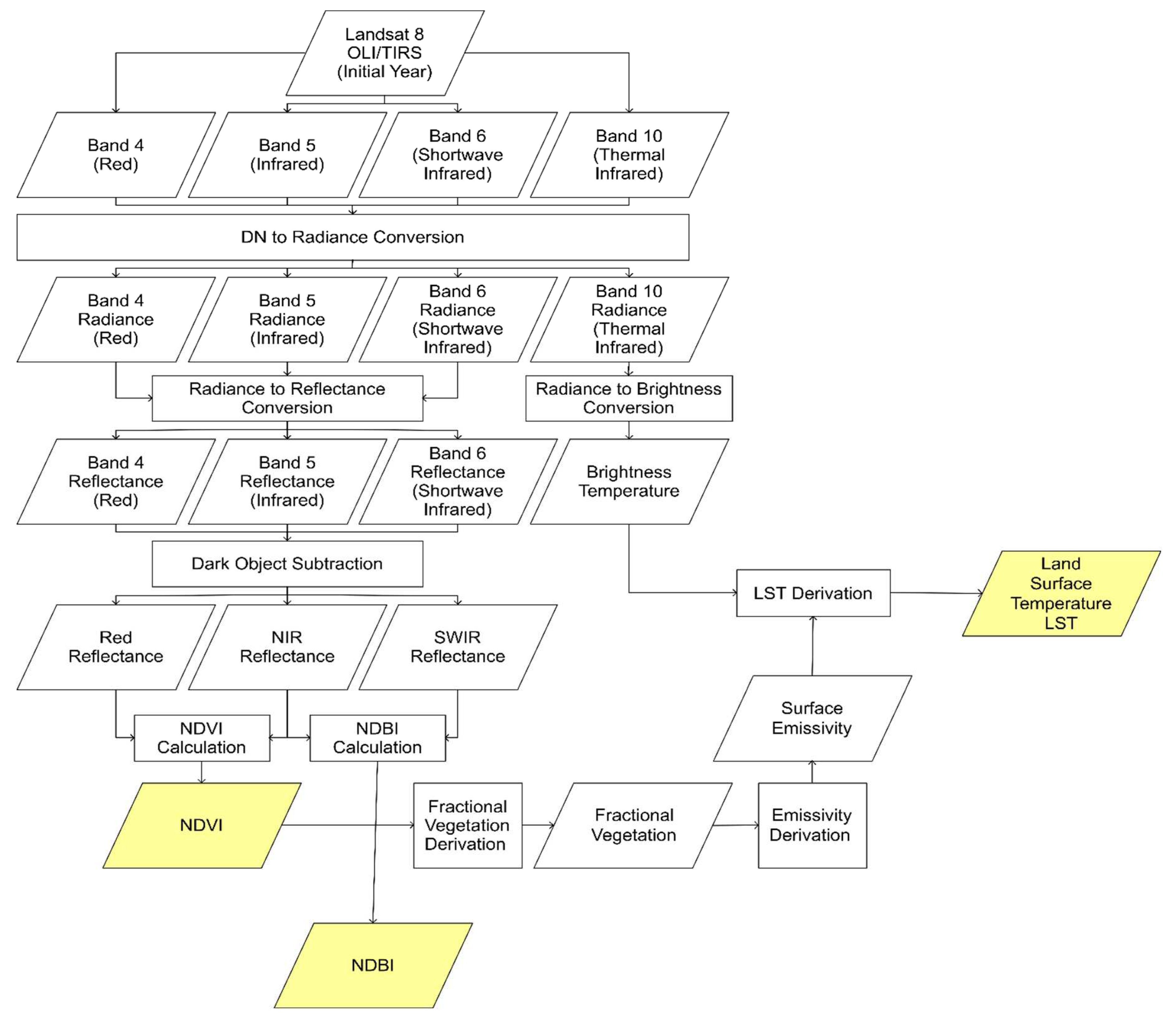
The research approach employed in this study for remote sensing digital image processing is illustrated in
Figure 3. This approach was applied for every Landsat 8 image used in this study. The borders of the study region were used to clip all Landsat images. The images were presented in the form of integer numbers known as digital numbers (DNs). The conversion process specified in the Landsat 8 Data User Handbook[
34] was used to convert the images to top-of-atmosphere (TOA) reflectance. As per this method, Landsat images were transformed from DN to at-sensor radiance using the following equation:
Where Lλ is the spectral at-sensor radiance, ML is the radiance multiplicative scaling factor for the band L, Qcal is the quantized calibrated pixel value, and AL is the radiance additive scaling factor for the band L.
The conversion from at-sensor radiance to top-of-atmosphere reflectance was achieved using the following equation:
Where ρλ is the unitless top-of-atmosphere (TOA) reflectance, d is the Earth-Sun distance measured in astronomical units ESUNλ is the mean solar exoatmospheric irradiances, and θs is the solar zenith angle.
The at-surface reflectance was derived using the dark object subtraction (DOS) method applied to the top-of-atmosphere (TOA) reflectance to eliminate atmospheric interference. The Dark Object Subtraction (DOS) is a straightforward and empirical technique used to remove atmospheric effects in remote sensing data. It operates under the assumption that the reflectance of dark objects contains a significant portion of atmospheric scattering. The DOS algorithm scans each band to identify the pixel with the lowest intensity and subsequently eliminates unwanted atmospheric distortions by removing this value from every pixel in the band [
35].
The NDVI, which stands for Normalized Difference Vegetation Index, is the predominant and extensively employed metric for vegetation extraction. This study utilized the NDVI as its primary index. The utilization of NDVI was initially employed for evaluating the existence of vegetation, a purpose that has been substantiated in several research [
36,
37]. NDVI is traditionally calculated by taking the ratio of at the surface red reflectance to near infrared reflectance as following equation:
The at-surface reflectance in the near infrared (NIR) and visible red (R) can be measured using band 5 and band 4 of Landsat 8 OLI.
The Normalized Difference Built-up Index (NDBI) is a spectral indicator designed for studying built-up areas. The calculation involves determining the ratio between the shortwave infrared (SWIR) and near-infrared (NIR) wavelengths. Areas with a dense built-up exhibit a greater reflection of shortwave-infrared (SWIR) radiation, whereas areas with less dense built-up display a lower level of reflectance in the near-infrared (NIR) spectrum [
38]. The calculation of NDBI was performed using the following equation [
39]:
In Landsat 8, band 5 and band 6 represent near infrared and shortwave infrared, and NDBI was obtained using at-surface reflectance.
To obtain the land surface temperature (LST) from Landsat 8 Band 10, the band was transformed into spectral at-sensor radiance using equation (1). This radiance was then utilized to derive the brightness temperature T
B in Kelvin using the following equation:
Where k1 and k2 are calibration constants that are equal 774.89 and 1321.08 respectively for Landsat 8 Band 10.
The surface emissivity (ε) was determined using the use of the NDVI thresholds approach [
40]. The fractional vegetation (Fv), which is defined as the proportion of the vertical projected area occupied by green vegetation to the total ground area, expressed as a percentage[
41], was calculated based on the Normalized Difference Vegetation Index (NDVI) using the following equation[
42]:
Where NDVImin refers to the minimum value of NDVI at which pixels are classified as bare soil, and NDVImax represents the maximum value of NDVI at which pixels are classified as healthy vegetation.
Land surface emissivity (ε
λ) is the measure of how effectively a surface releases heat radiation. ε
λ is a quantitative assessment of a surface's ability to emit heat by infrared radiation, relative to a perfect emitter called a blackbody. In theory, the ε
λ of a surface is commonly quantified as a numerical number ranging from 0 to 1. A value of 0 signifies a surface that perfectly reflects radiation without emitting any, while a value of 1 indicates a surface that fully emits radiation. ε
λ is necessary for the estimation of land surface temperature. The equation provided was used to calculate the emissivity of the land surface[
43]:
Where ε
vλ and ε
sλ are the emissivity of a full vegetative surface and full soil surface respectively. δ
λ is the surface roughness that is considered as a constant value of 0.005[
44]. Practically, equation (7) adopted to the following form[
45]:
When the NDVI falls below 0, pixel is considered water with an emissivity value of 0.991. NDVI values ranging from 0 to 0.2 indicate soil coverage and are assigned an emissivity value of 0.996. The range of NDVI values between 0.2 and 0.5 is classified as a combination of soil and vegetation cover, and the equation (8) is utilized to extract the emissivity. When the NDVI value exceeds 0.5 in the last scenario, it is classified as vegetation-covered and assigned a value of 0.973.
Finally, land surface temperature (LST) is derived using the following equation:
Where λ is the effective wavelength which is 10.9 mm for Landsat 8's band 10, ρ is Boltzmann constant (1.38 × 10⁻²³ J/K), h is Plank’s constant (6.626 × 10⁻³⁴ Js), c is the light's velocity (2.998 × 10⁻⁸ m/sec) and ελ is emissivity.
LST
k is obtained in Kelvin, then converted to Celsius using the following equation:
Where LSTc is the land surface temperature in Celsius.
A total of one thousand random locations were produced to encompass the whole study area. The points were utilized to gather the measurements of NDVI, NDBI, and LSTc at their respective positions. The sampling results were exported to Minitab (
https://www.minitab.com/) to examine the correlation between NDVI and LSTc, as well as between NDBI and LSTc, both before and after the development of the study area. Three hypotheses were examined:
- ■
Hypothesis 1 (H1): Normalized Difference Vegetation Index (NDVI) has a substantial impact on Land Surface Temperature (LST) in the study area before and after the development.
- ■
Hypothesis 2 (H2): The Normalized Difference Built-up Index (NDBI) exerts a substantial impact on Land Surface Temperature (LSTc) across the study area before and after the development.
- ■
Hypothesis 3 (H3): The variables NDVI and NDBI have a considerable impact on Land Surface Temperature Change (LSTc).
Results
Spatiotemporal Pattern of NDVI and NDBI
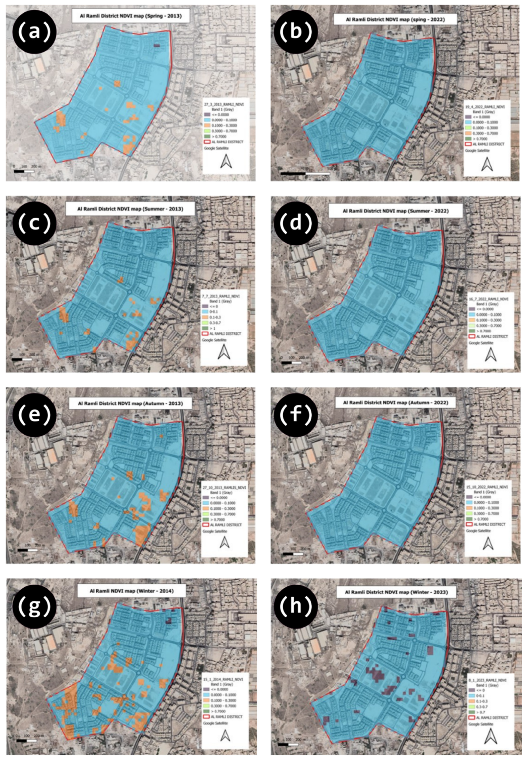
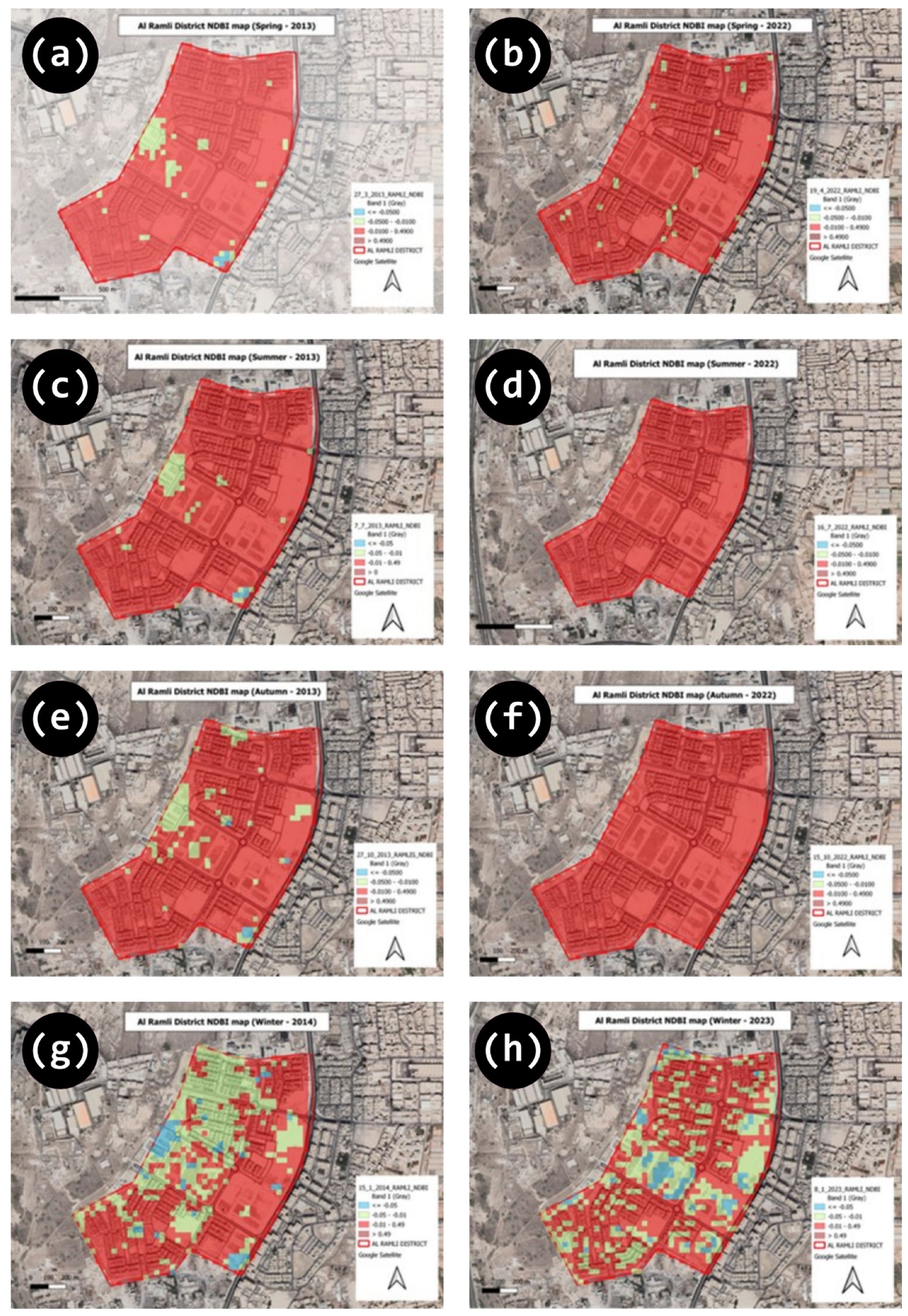
NDVI is a quantitative measure employed to evaluate and track the quantity of thriving vegetation inside a certain region. The spatial distribution of NDVI over the study period is depicted in
Figure 4, while
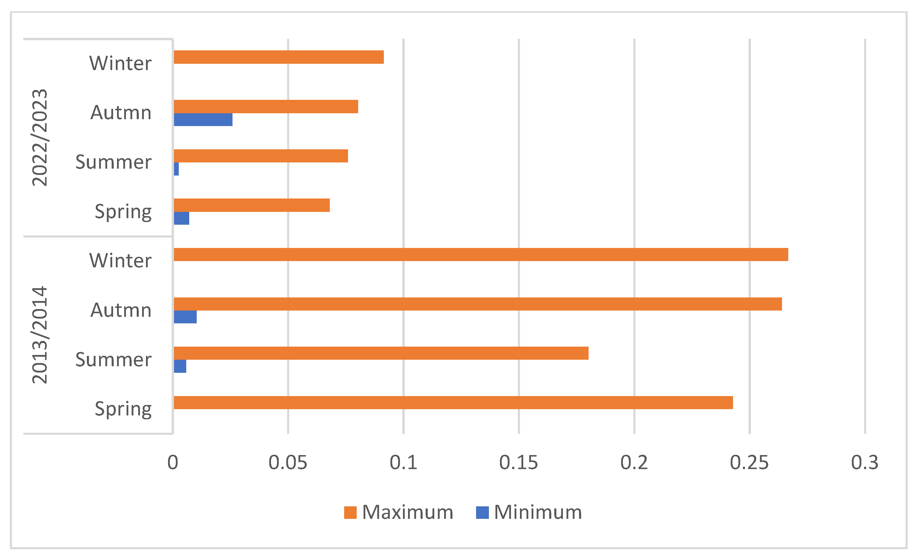
Figure 5 illustrates the seasonal fluctuations of NDVI. The NDVI values in the years 2022–2023 exhibit a decrease as compared to the years 2013–2014. The average difference in NDVI values during the years dropped by 0.028, 0.0177, 0.0235, and 0.0534, respectively. The lowest NDVI value was seen during the winter of 2014 and 2023. Conversely, the highest NDVI value was recorded during the winter of 2014, reaching 0.2667.
Researchers observed that the primary land use in the study area is characterized by medium-density residential development.
Figure 6 displays the alterations in spatial patterns of NDBI, whereas
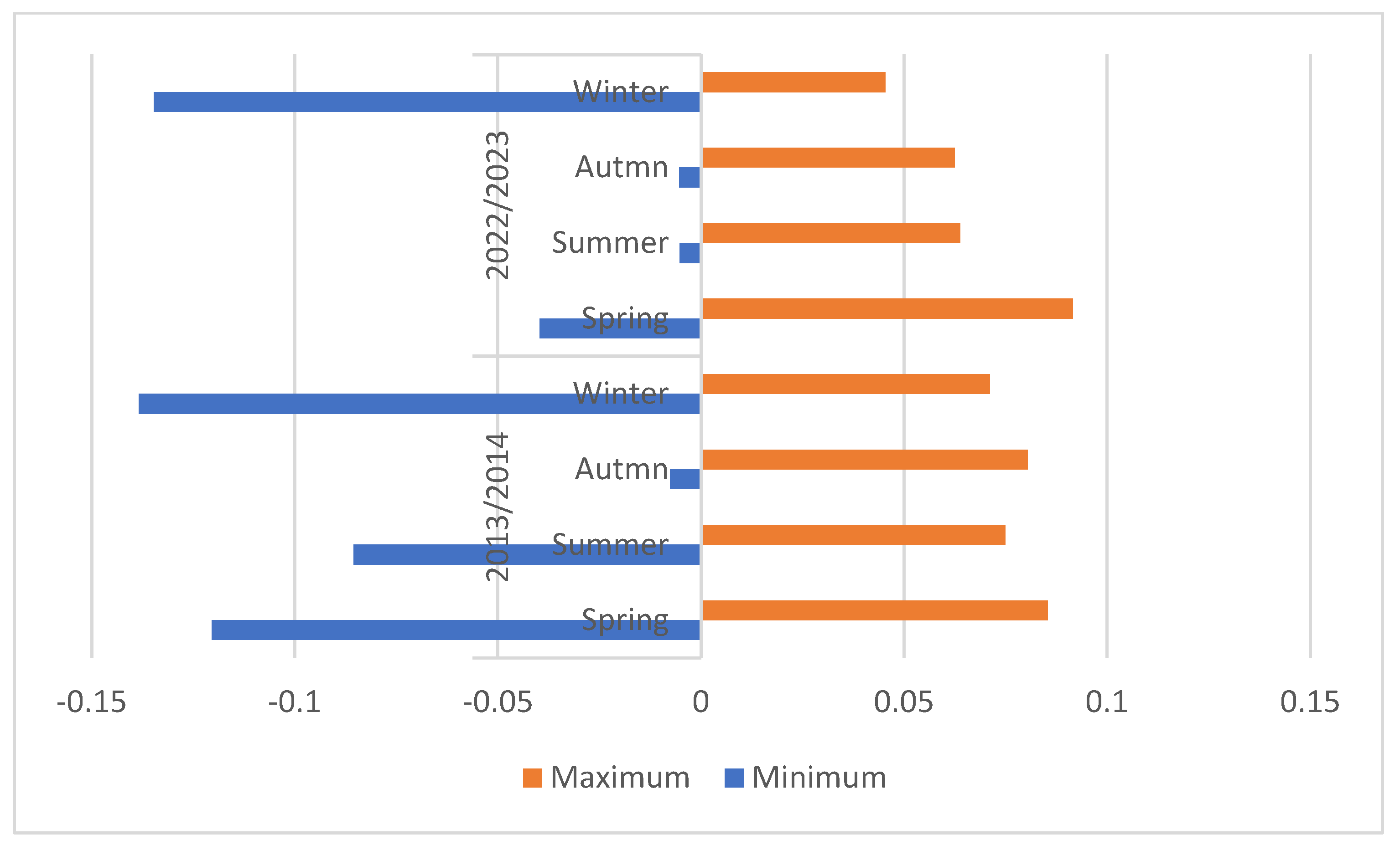
Figure 7 illustrates the seasonal fluctuations of NDBI before and after the development of the study area. The Normalized Difference Built-up Index (NDBI) is a spectral index employed in remote sensing to detect and measure the extent of developed or urban regions in a given area. The highest recorded value of the NDBI occurred during the spring of 2022, at 0.0916. The mean values in the four seasons differed by 0.0002, 0.0046, 0.0042, and 0.0052, respectively, suggesting that there is no substantial variation in NDBI among years.
Spatiotemporal Pattern of Land Surface Temperature
Land surface temperature (LST) was derived using data from Band 10 of the Landsat 8 OLI/TIRS satellite for both the pre- and post-development periods of the study area.
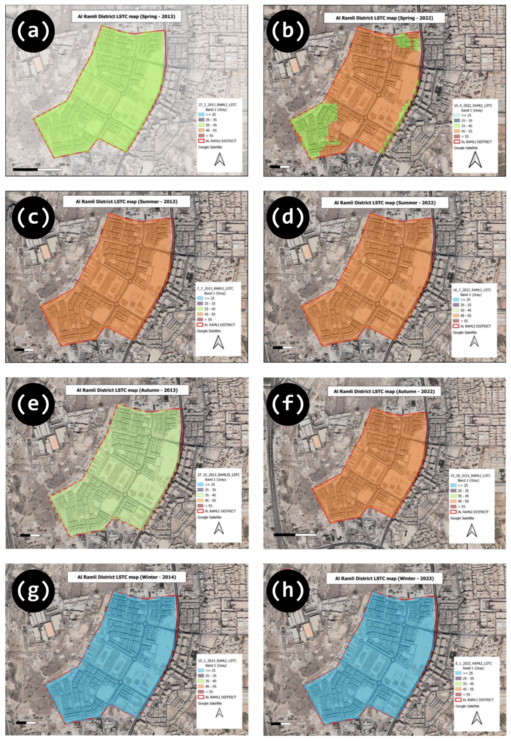
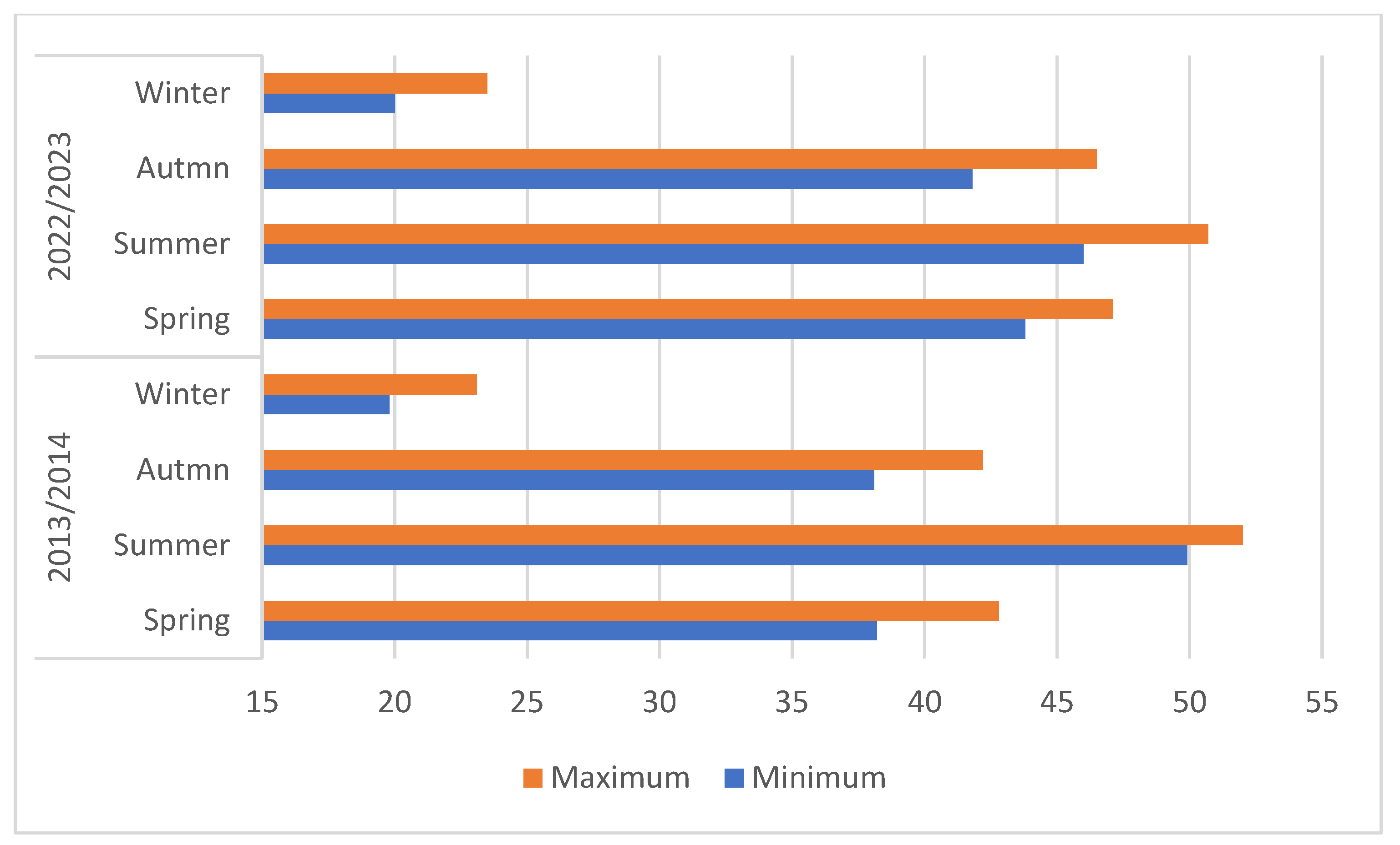
Figure 8 displays the categorized land surface temperature maps of the study area for the four seasons in the years 2013-2014 and 2022-2023. The LST maps identified a rise in springtime LST, with the temperature in 2013 being categorized as high. The maximum and minimum temperatures recorded were 42.8°C and 38.2°C, respectively. In 2022, most of the study area was categorized as having a very high LST, with some areas experiencing high LST. The highest recorded LST was 47.1°C, while the lowest was 43.8°C. In fall 2013, the temperature ranged from a maximum of 42.2°C to a minimum of 38.1°C, with a high LST classification. However, in 2022, the LST is significantly higher, with a maximum of 50.7°C and a minimum of 46°C. The LST classification remained unchanged during both the summer and winter seasons. The summer season was categorized as having extremely high LST, whereas the winter season was categorized as having moderate LST. The seasonal variation of land surface temperature LST pre- and post- development of the study area is shown in
Figure 9.
Modeling relationships between NDVI, NDBI, and LST
To assess, one can establish the correlation between the Normalized Difference Vegetation Index (NDVI) and Land Surface Temperature (LST), as well as the correlation between the Normalized Difference Built-up Index (NDBI) and LST, by doing a linear regression analysis. During the regression test, the LST will serve as the response variable (dependent variable), while the NDVI and NDBI will be used as predictor variables (independent variables). Both NDVI and NDBI values were derived from the analysis of Landsat 8-9 OLI / TIRS C2 L2 data.
The subsequent results will delve into the variations in LST, NDVI, and NDBI. Furthermore, it will explore the impact of NDVI and NDBI on LST across all four seasons within the study area.
The subsequent outcomes considered the following hypotheses:
- ■
Hypothesis 1: NDVI has a substantial impact on LST in the study area.
- ■
Hypothesis 2: NDBI has a significant impact on LST.
- ■
Hypothesis 3: Both the NDVI and NDBI variables have a significant impact on LST.
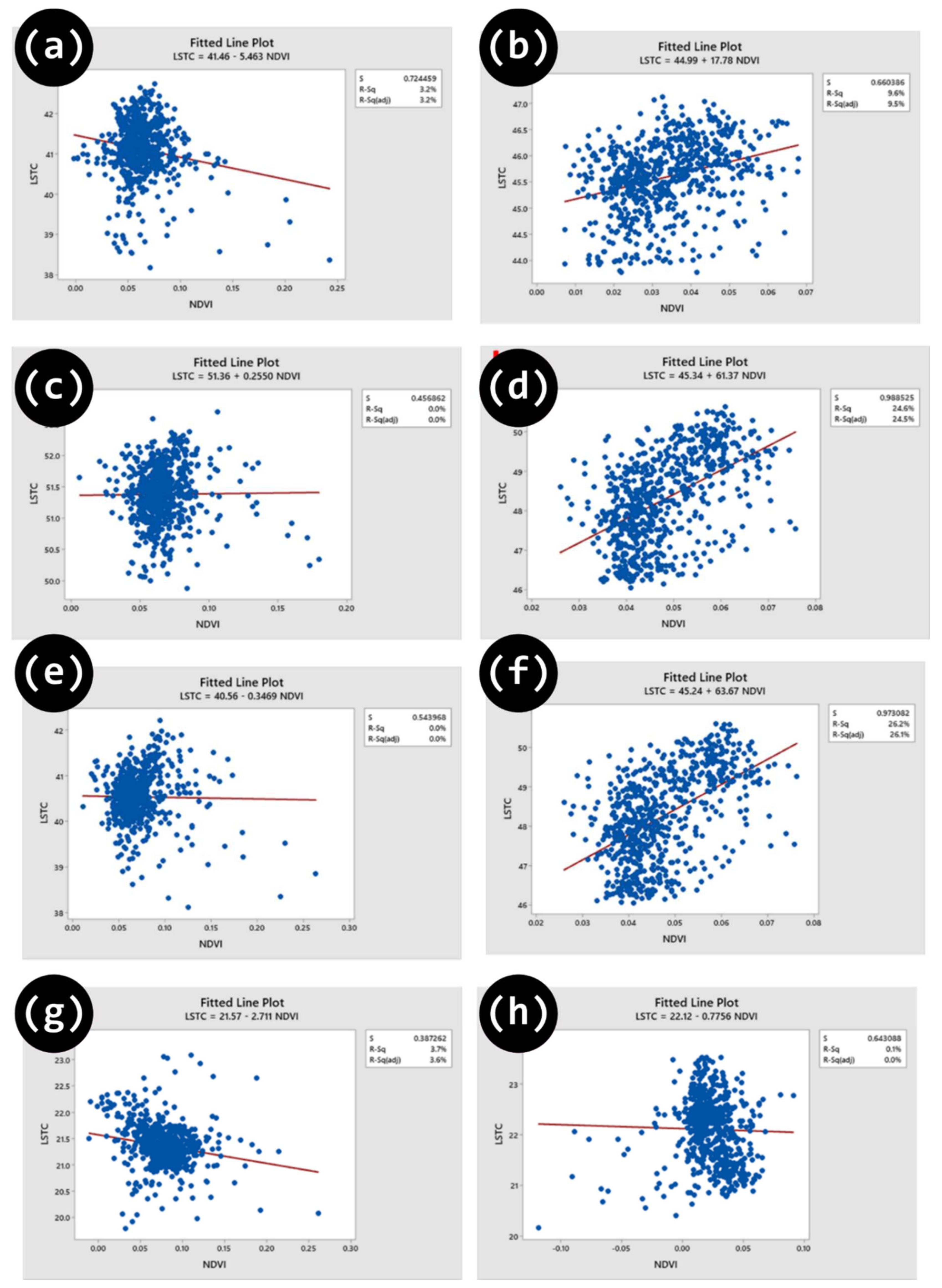
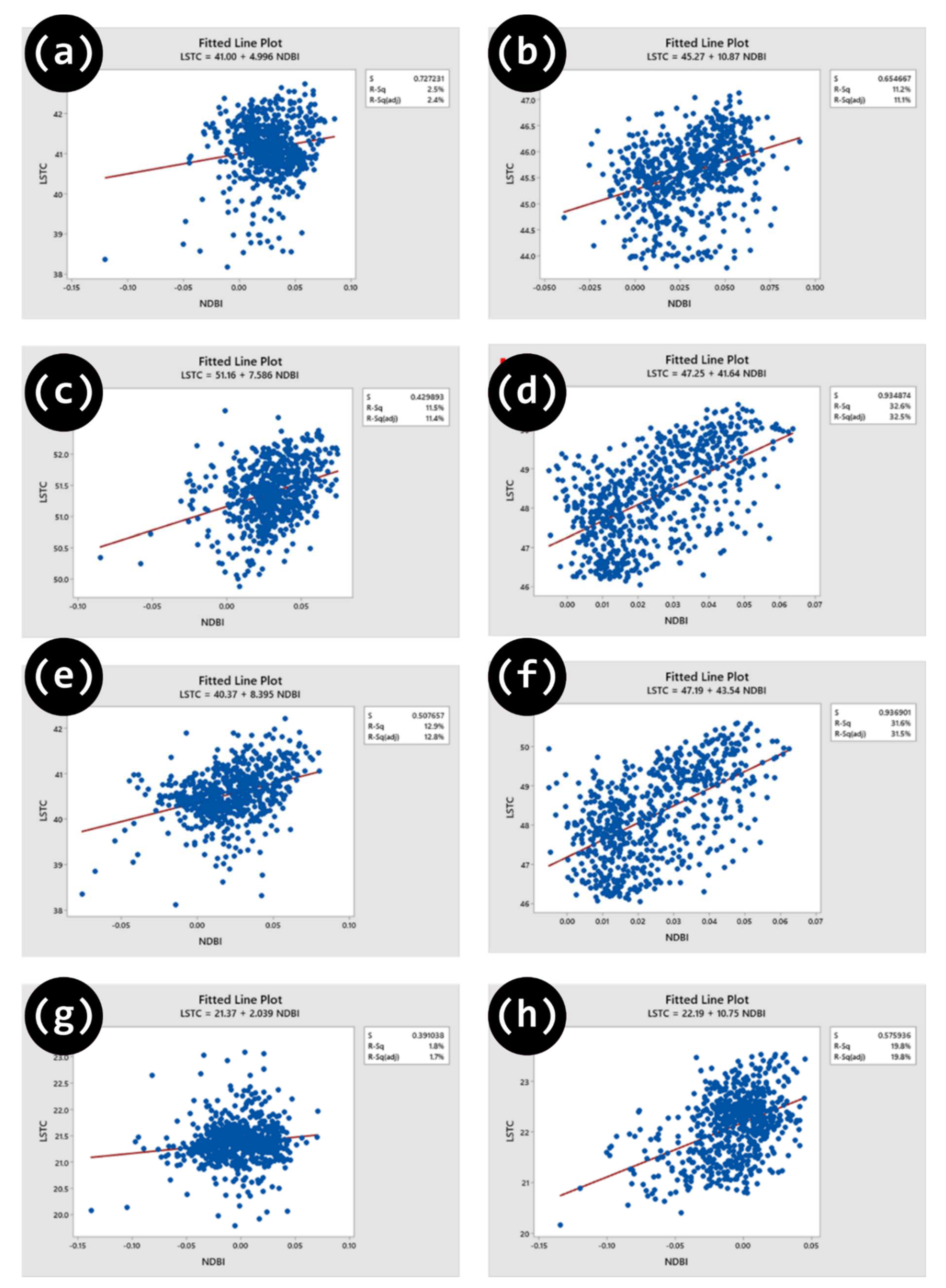
In order to examine the association between NDBI, NDVI, and LST in the study area, a total of 1000 randomly selected sample points were taken from NDBI, NDVI, and LST datasets. These sample points were then utilized to conduct regression analysis. The coefficient of determination (R²) and Pearson correlation coefficients were obtained to assess the strength of the relationships. The linear regression models for NDVI and LST, as well as for NDBI and LST, are shown in
Figure 10 and
Figure 11 respectively.
There is a significant and consistent positive relationship between NDBI and land surface temperature at a 95% confidence level over four seasons in the years 2013–2014 and 2022–2023. The Pearson index values for the years 2013-2014 were 0.158, 0.339, 0.360, and 0.135, respectively. For the years 2022-2023, the Pearson index values were 0.334, 0.571, 0.562, and 0.445, respectively. For each incremental rise of 0.01 in the NDBI value, the land surface temperature experienced corresponding increases of 0.05 °C, 0.08 °C, 0.08 °C, and 0.02 °C in the years 2013-2014. In the years 2022-2023, the land surface temperature would climb by 0.11 °C, 0.42 °C, 0.44 °C, and 0.11 °C, correspondingly, for the same incremental increase in NDBI value. The correlation between NDBI and LST indicates a consistent rise in the NDBI index throughout time. NDBI successfully identified and described the variations in LST.
Figure 10 shows a negative association between NDVI and LST in various seasons. For each 0.01 rise in NDVI value, the equivalent LST in four seasons during 2013-2014 (except summer) reduced by 0.06 °C, 0.0003 °C, and 0.03 °C, respectively. In the summer season, the LST increased by 0.0025 °C. During the period of 2022-2023, the LST is projected to rise by 0.18 °C, 0.61 °C, and 0.64 °C, respectively, and experience a decrease of 0.01 °C during the winter season. Hence, the NDVI index exhibited sensitivity towards variations in LST, and any disagreement in the NDVI could potentially lead to a modification in LST. NDVI and LST exhibited a negative correlation during the spring, fall, and winter seasons of 2013-2014. The Pearson coefficient, calculated at a 95% level of confidence, was determined to be -0.18, -0.016, and -0.192, respectively. In the summer, there was a positive correlation between the variables, as indicated by a Pearson value of 0.01. In contrast, over the period of 2022-2023, there was a positive correlation between NDVI and LST in spring, summer, and fall. This correlation was statistically significant at a 95% confidence level, with Pearson coefficients of 0.310, 0.496, and 0.512, respectively. The association exhibited a negative correlation throughout the winter season, with a Pearson coefficient of -0.025. However, despite the shifting seasons, the correlation between NDVI and LST was not consistent.
During the year of 2013-2014, there was a negative connection between NDBI and NDVI in the seasons of spring, summer, and winter. The Pearson index values for these seasons were -0.16, -0.076, and -0.147 respectively. However, in the autumn season, there was a positive correlation with a Pearson index value of 0.021. In addition, throughout the period of 2022-2023, there was a strong positive association seen between NDBI and NDVI in all four seasons. The Pearson index values were 0.286, 0.663, 0.62, and 0.24. The correlation between NDVI and land utilization for urban construction was evident, as it accurately depicted the changes that occurred over time.
Conclusion
This study employed Landsat 8 OLI/TIRS images to examine the correlation between urban development and temperature fluctuations, using Normalized Difference Vegetation Index (NDVI), Normalized Difference Built-up Index (NDBI), and Land Surface Temperature (LST) as primary indicators. The study area was situated in the Kingdom of Bahrain, and the analysis was conducted during the period of 2013-2023. The urban growth in the study area was assessed based on the results of the NDBI. Urban expansion has created additional residential space, albeit it has come at the expense of the natural environment. The LST exhibited significant rises throughout the summer months following urban growth, in contrast to the period before development. The mean LST increased from 41.1°C to 45.6°C during Spring and from 40.5°C to 44.2°C during Autumn following the implementation of urban growth in the studied area. In this overall pattern, the land surface temperature (LST) of the study area experienced a more noticeable increase.
Using Bahrain as an example of a city in the Gulf Cooperation Council (GCC) that has seen population increase and urban expansion, it is probable that the tendency of the study area's population increasing in conjunction with the LST will persist. It is highly likely that this could have multiple harmful impacts on the urban runoff pattern, climate conditions, and the livable environment. Prior to any additional alterations to its unorganized constructed surroundings, the city necessitates the focus of urban planners and policymakers to prevent any distortion in LST patterns.
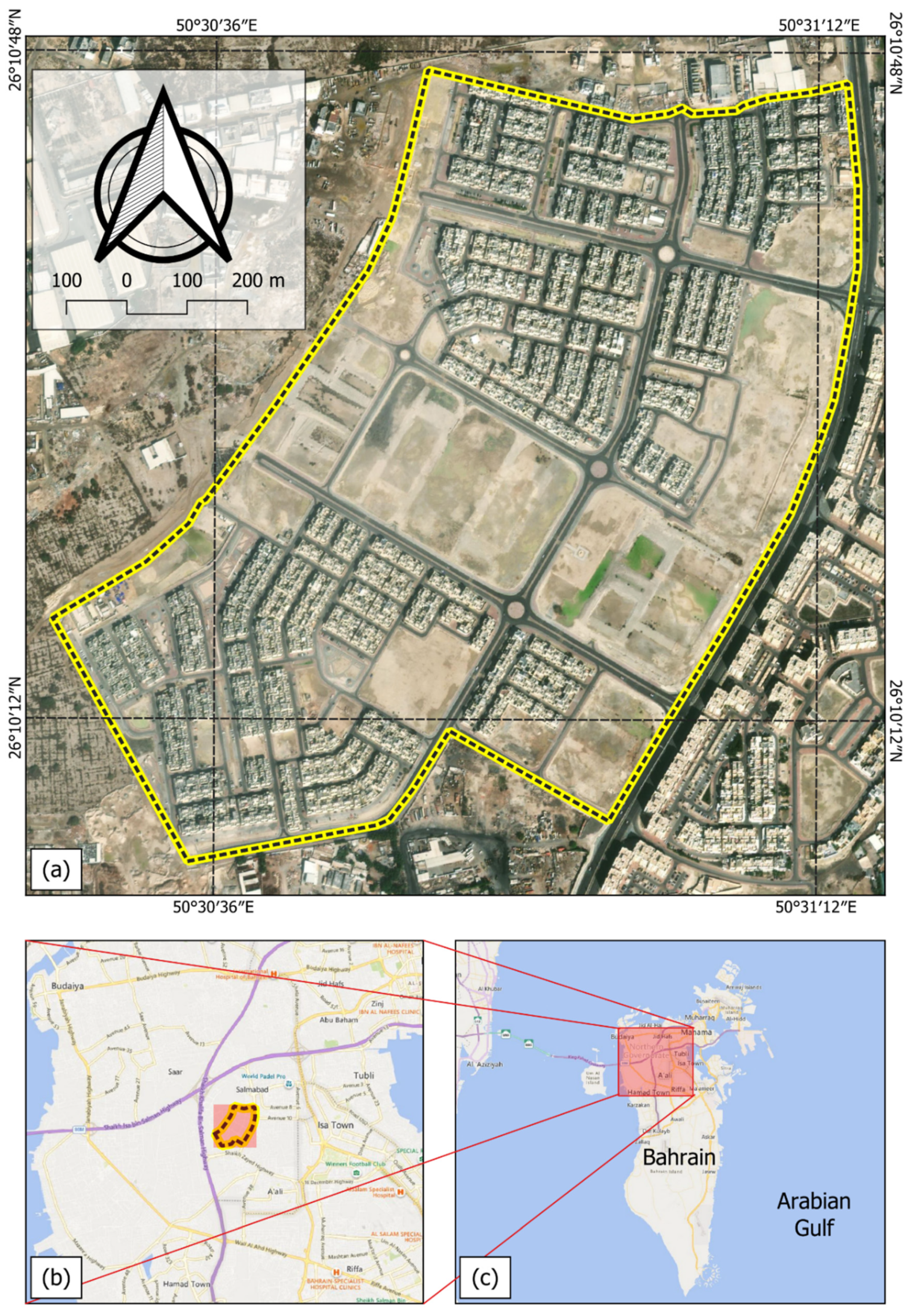
Figure 1.
Location of the study area.
Figure 1.
Location of the study area.
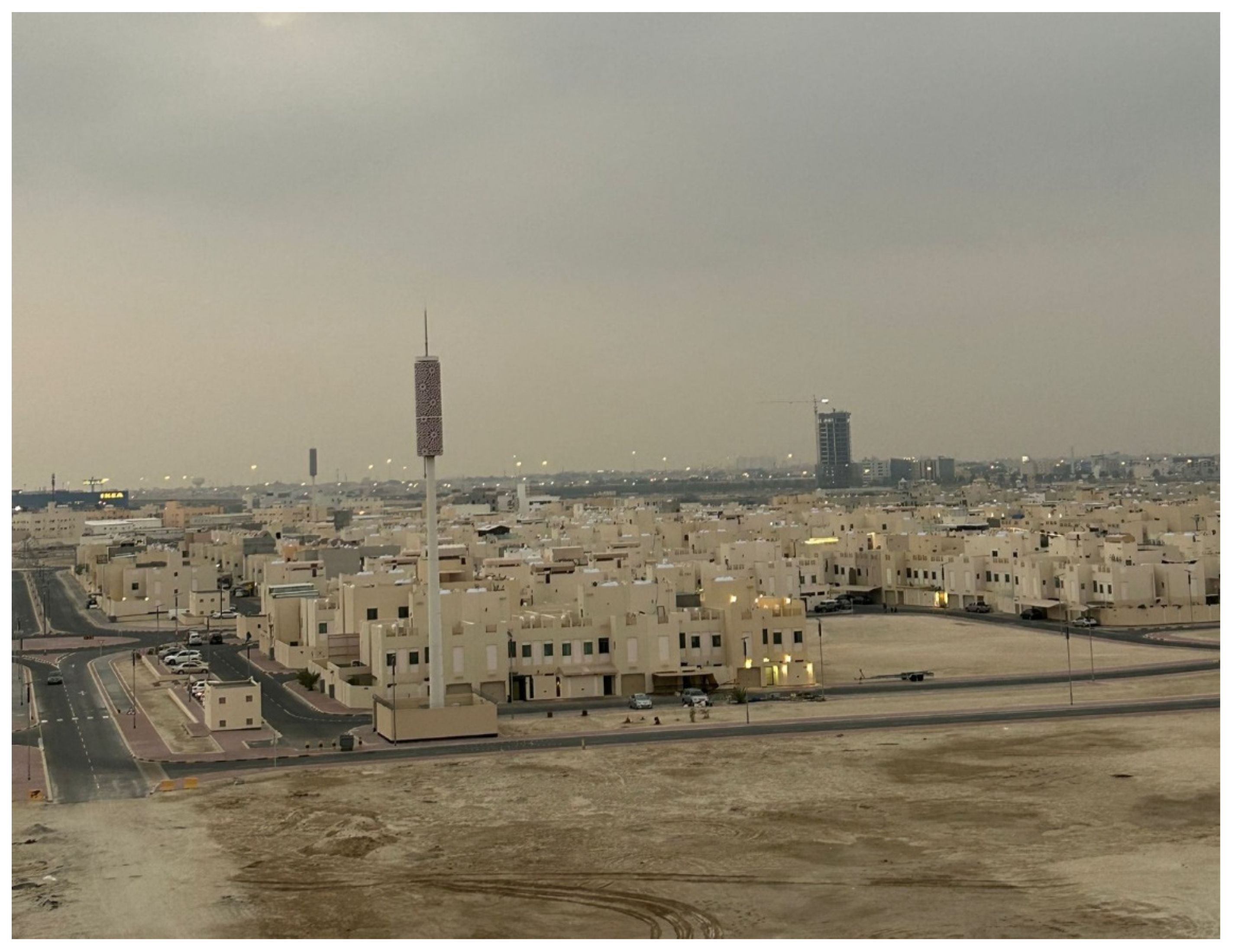
Figure 2.
A photo of the study area.
Figure 2.
A photo of the study area.
Figure 3.
Flowchart for the methodology of the study.
Figure 3.
Flowchart for the methodology of the study.
Figure 4.
Spatial pattern of NDVI over the study area at (a) Spring 2013, (b) Spring 2022, (c) Summer 2013, (d) Summer 2022, (e) Autmn 2013, (f) Autmn 2022, (g) Winter 2014, and (h) Winter 2023.
Figure 4.
Spatial pattern of NDVI over the study area at (a) Spring 2013, (b) Spring 2022, (c) Summer 2013, (d) Summer 2022, (e) Autmn 2013, (f) Autmn 2022, (g) Winter 2014, and (h) Winter 2023.
Figure 5.
Seasonal variation of land surface temperature NDVI before and after development of the study area.
Figure 5.
Seasonal variation of land surface temperature NDVI before and after development of the study area.
Figure 6.
Spatial pattern of NDBI over the study area at (a) Spring 2013, (b) Spring 2022, (c) Summer 2013, (d) Summer 2022, (e) Autmn 2013, (f) Autmn 2022, (g) Winter 2014, and (h) Winter 2023.
Figure 6.
Spatial pattern of NDBI over the study area at (a) Spring 2013, (b) Spring 2022, (c) Summer 2013, (d) Summer 2022, (e) Autmn 2013, (f) Autmn 2022, (g) Winter 2014, and (h) Winter 2023.
Figure 7.
Seasonal variation of land surface temperature NDBI before and after development of the study area.
Figure 7.
Seasonal variation of land surface temperature NDBI before and after development of the study area.
Figure 8.
Spatial pattern of LST over the study area at (a) Spring 2013, (b) Spring 2022, (c) Summer 2013, (d) Summer 2022, (e) Autmn 2013, (f) Autmn 2022, (g) Winter 2014, and (h) Winter 2023.
Figure 8.
Spatial pattern of LST over the study area at (a) Spring 2013, (b) Spring 2022, (c) Summer 2013, (d) Summer 2022, (e) Autmn 2013, (f) Autmn 2022, (g) Winter 2014, and (h) Winter 2023.
Figure 9.
Seasonal variation of land surface temperature LST before and after development of the study area.
Figure 9.
Seasonal variation of land surface temperature LST before and after development of the study area.
Figure 10.
Regression models for NDVI and LST at (a) a) Spring 2013, (b) Spring 2022, (c) Summer 2013, (d) Summer 2022, (e) Autmn 2013, (f) Autmn 2022, (g) Winter 2014, and (h) Winter 2023.
Figure 10.
Regression models for NDVI and LST at (a) a) Spring 2013, (b) Spring 2022, (c) Summer 2013, (d) Summer 2022, (e) Autmn 2013, (f) Autmn 2022, (g) Winter 2014, and (h) Winter 2023.
Figure 11.
Regression models for NDBI and LST at (a) a) Spring 2013, (b) Spring 2022, (c) Summer 2013, (d) Summer 2022, (e) Autmn 2013, (f) Autmn 2022, (g) Winter 2014, and (h) Winter 2023.
Figure 11.
Regression models for NDBI and LST at (a) a) Spring 2013, (b) Spring 2022, (c) Summer 2013, (d) Summer 2022, (e) Autmn 2013, (f) Autmn 2022, (g) Winter 2014, and (h) Winter 2023.
Table 1.
Dates of obtained Landsat 8 OLI/TIRS images.
Table 1.
Dates of obtained Landsat 8 OLI/TIRS images.
| Season |
before development |
after development |
| Spring |
27/03/2013 |
19/04/2022 |
| Summer |
07/07/2013 |
16/07/2022 |
| Autumn |
27/10/2013 |
15/10/2022 |
| Winter |
15/01/2014 |
08/01/2023 |
