1. Introduction

2. Revisiting Materials and Methods

2.1. FRAP Experiments

Here we consider FRAP experiments [50] where NS5A proteins are marked by fluorescent dye. The proteins reside on the ER surface in liver cells. The cell is prepared in a state where the protein is distributed (and fluoresces) homogeneously. In Fig. 1 the ER appears as a bicontinuous structure colored in red and blue. The ER has a height of a few pore diameters and large lateral extension. The experiment starts by applying a bright laser pulse applied to a small and sharply confined spatial region. In Fig. 1 this region is colored in red. The pulse bleaches the dye and hence quenches the fluorescence in this region. In the following these regions will be denoted as the FRAP region of interest (FRAP ROI) $\mathcal{F}$. This region has the shape of a cylinder, with a height that amounts to the thickness of the ER, $H\simeq 3.5\mathsf{\mu }\mathrm{m}$, and a circular cross section of $A=\pi R^2$ with $R\simeq 3.5\mathsf{\mu }\mathrm{m}$.

Figure 1. Surface mesh of a reconstructed ER geometry. (a) Computational domain used for the simulations of the FRAP experiments of NS5A. The displayed ER has a maximum thickness of about $4.8\mathsf{\mu }\mathrm{m}$, which amounts to only a few pore diameters, and the present view has a lateral extension of $46\mathsf{\mu }\mathrm{m}\times 46\mathsf{\mu }\mathrm{m}$. The unbleached region $\mathcal{U}$ is displayed in dark blue, and the FRAP region $\mathcal{F}$ used for bleaching in red. (b) Magnification around the FRAP region $\mathcal{F}$ with an extension of $19.2\mathsf{\mu }\mathrm{m}\times 10.9\mathsf{\mu }\mathrm{m}$, and a maximum thickness of about $3.5\mathsf{\mu }\mathrm{m}$. The FRAP region $\mathcal{F}$ has a surface area of $A=38\mathsf{\mu }{\mathrm{m}}^2\simeq \pi {\left(3.5\mathsf{\mu }\mathrm{m}\right)}^2$ in the 2D projection plane. The table provides the relevant properties of the reconstructed ER geometries adopted in the present study. Details on the reconstruction and representation of the surface meshes are provided in [45].

Figure 1. Surface mesh of a reconstructed ER geometry. (a) Computational domain used for the simulations of the FRAP experiments of NS5A. The displayed ER has a maximum thickness of about $4.8\mathsf{\mu }\mathrm{m}$, which amounts to only a few pore diameters, and the present view has a lateral extension of $46\mathsf{\mu }\mathrm{m}\times 46\mathsf{\mu }\mathrm{m}$. The unbleached region $\mathcal{U}$ is displayed in dark blue, and the FRAP region $\mathcal{F}$ used for bleaching in red. (b) Magnification around the FRAP region $\mathcal{F}$ with an extension of $19.2\mathsf{\mu }\mathrm{m}\times 10.9\mathsf{\mu }\mathrm{m}$, and a maximum thickness of about $3.5\mathsf{\mu }\mathrm{m}$. The FRAP region $\mathcal{F}$ has a surface area of $A=38\mathsf{\mu }{\mathrm{m}}^2\simeq \pi {\left(3.5\mathsf{\mu }\mathrm{m}\right)}^2$ in the 2D projection plane. The table provides the relevant properties of the reconstructed ER geometries adopted in the present study. Details on the reconstruction and representation of the surface meshes are provided in [45].

After bleaching the diffusive rearrangement of NS5A between the region and its environment is recorded by tracking the recovery of fluorescence. Fluorescence recovers due to the influx of NS5A proteins labeled with operational dye molecules from the surrounding unbleached region $\mathcal{U}$. The recovery is followed by inducing dye fluorescence by repetitive application of a second (soft) laser beam. Representative measurement signals are shown by the data points in Fig. 2. The initial recovery up to a level of $0.35$ proceeds within a few seconds. Subsequently, the experimental signal keeps rising slowly. However, even the soft laser beam causes photobleaching, and this photobleaching is slowly extinguishing the fluorescence signal. Full details are provided in Ref. [45].

Figure 2. Experiment (dots) and simulations (solid lines) of the FRAP signal for two different cell lines where one expects different surface diffusivities D. The blue and red lines show simulation results where photobleaching is neglected and for a finite quench rate, respectively. The geometry of the ER of the cells used in the experiments is not known. The simulations were performed for the geometry M4a (left) and M1a (right), respectively. The initial conditions and parameters adopted in the simulations are provided in the table below the plots. [The Figure was initially published as Fig. 5 and Fig. 6 in Ref. [45].

Figure 2. Experiment (dots) and simulations (solid lines) of the FRAP signal for two different cell lines where one expects different surface diffusivities D. The blue and red lines show simulation results where photobleaching is neglected and for a finite quench rate, respectively. The geometry of the ER of the cells used in the experiments is not known. The simulations were performed for the geometry M4a (left) and M1a (right), respectively. The initial conditions and parameters adopted in the simulations are provided in the table below the plots. [The Figure was initially published as Fig. 5 and Fig. 6 in Ref. [45].

Numerical tests of our theoretical considerations will be compared to simulations performed for diffusion on reconstructions of the ER geometry. An example is provided in Fig. 1. The ER geometries will be denoted as M1 to M5. For each of them we consider 2 distinct locations of the FRAP region of interest. This distinction will be marked by a and b, respectively. Hence, for the simulations we consider 10 ER structures in total. Moreover, in order to explore the impact of the bicontinuous structure of the ER, we also perform simulations on a flat disk. This structures will be denoted as disk. The relevant material parameters of the structures are provided in the table in Fig. 1. A detailed description of the structures and the numerical method has been provided in Ref. [45].

2.2. Mathematical Model of NS5A Diffusion

We express the dynamics of NS5A fluorescence in terms of the intensity density that is proportional to the concentration $c_{\mathrm{ns}5\mathrm{a}}(t,\mathbf{x})$ anchored in the ER. We consider 5 ER geometries that are reconstructed based on experimental data. The surfaces are represented as triangulated manifolds with a resolution of about ${10}^6$ nodes [45]. Fig. 1 shows an example of such a geometric setup. The ER [25,58,59] comprises a bicontinuous structure with a characteristic pore diameter of 1 $\mathsf{\mu }\mathrm{m}$. It has a thickness of a few pore diameters, and a lateral extension of about 50 pore diameters in the other two directions. The overall surface area of the membrane comprising the ER is of the order of $\left|\mathcal{U}\right|\simeq 5000\mathsf{\mu }{\mathrm{m}}^2$. The specific values for the structures considered in the present study are provided in the table in Fig. 1. Full details concerning the investigated structures are provided in [43,45,46].

The evolution of the protein on the ER surface domain is described by a surface PDE (sufPDE) where the Laplace-Beltrami operator ${\Delta }_{\left(\mathrm{T}\right)}$ is the projection of the Laplace operator to the tangential space of the two dimensional ER-hypersurface $\mathcal{F}\cup \mathcal{U}$. It models diffusion, analogously to a Laplace operator for diffusion in Euclidean space. The right-hand side of the equation accounts for the intensity reduction due to quenching of the dye in the course of the the intensity measurement with the soft laser.

The present analysis is adopting simulations without quenching $r_p=0{\mathrm{s}}^{-1}$, and with a quench rate $r_p\simeq 0.0020{\mathrm{s}}^{-1}$ that is slightly larger than the values $0.0011{\mathrm{s}}^{-1}$ and $0.0016{\mathrm{s}}^{-1}$ reported for NS5A/Alone and NS5A/OtherNSPs cells, respectively [45].

The surface diffusion coefficient is varied in the range of $5\times {10}^{-4}$ ...$1\times {10}^{-1}\mathsf{\mu }{\mathrm{m}}^2/\mathrm{s}$. In order to match the experimental setup, initial conditions for Eq. (1) are provided independently for the bleached ($\mathcal{F}$) and unbleached ($\mathcal{U}$) regions

For the comparison with the experimental intensity in $\mathcal{F}$, we define the integrated normalized luminosity where dS denotes surface area elements on the ER.

Figure 3 displays a screenshot of a simulation movie for the NS5A dynamics on the ER surface mimicking a FRAP experiment. The simulation movie itself is attached as supplemental movie to this study.

Figure 3. Screenshot of the evaluation of NS5A FRAP experiment simulation based on sufPDE description, Eq. (1), on an ER surface: (left) total view, (right) zoom into FRAP ROI event. The complete movie is attached as supplemental material to this study.

Figure 3. Screenshot of the evaluation of NS5A FRAP experiment simulation based on sufPDE description, Eq. (1), on an ER surface: (left) total view, (right) zoom into FRAP ROI event. The complete movie is attached as supplemental material to this study.

3. Scaling Analysis

3.1. Scaling Analysis of the FRAP ROI Intensity

In order to discuss the solutions of Eq. (1) we introduce the surface area in the hole, and the space-dependent absorption rate where $\ell \left(\mathbf{x}\right)$ is the signed distance of $\mathbf{x}$ to the boundary $\partial \mathcal{F}$ of $\mathcal{F}$ (with negative values denoting positions inside $\mathcal{F}$), and

With these we write Eq. (1) as

Multiplying by $exp\left(\gamma \left(\mathbf{x}\right)t\right)$, dividing by $\mathcal{A}=\left|\mathcal{F}\right|$, and integrating both parts over $\mathcal{F}\cup \mathcal{U}$ provides

Here we first used that $\gamma \left(\mathbf{x}\right)=r_p$ takes a constant value on $\mathcal{F}$, and then we adopted Gauss’s theorem to express the integral over $\mathcal{F}\cup \mathcal{U}$ as an integral over its surface $\partial \mathcal{F}$.

Equation (5) must be solved for the initial condition

3.2. Scaling for Negligible Photobleaching

In the absence of photobleaching, $r_p\simeq 0$, Equation (5) reduces to

We non-dimensionalize the equations by adopting the radius R of the FRAP region as length scale and the dimensionless time $\tau =D(t-t_0)/R^2$. Moreover, we note that the equations (Section 3.2) are liner. As a consequence, there is a superposition principle and one can account for the different values of $i_0^{\mathcal{U}}$ and $i_0^{\mathcal{F}}$ in the initial condition by considering the normalized intensity $\tilde{I}\left(\tau \right)=(I\left(t\right)-I_0)/\left(|i_0^{\mathcal{U}}-i_0^{\mathcal{F}}|\right)$ (see the chapter on Greens functions in Ref. [60]).1 As a consequence, the reduced intensity takes same evolution for every geometry of the ER, irrespective of the value of the diffusion coefficient and the initial condition.

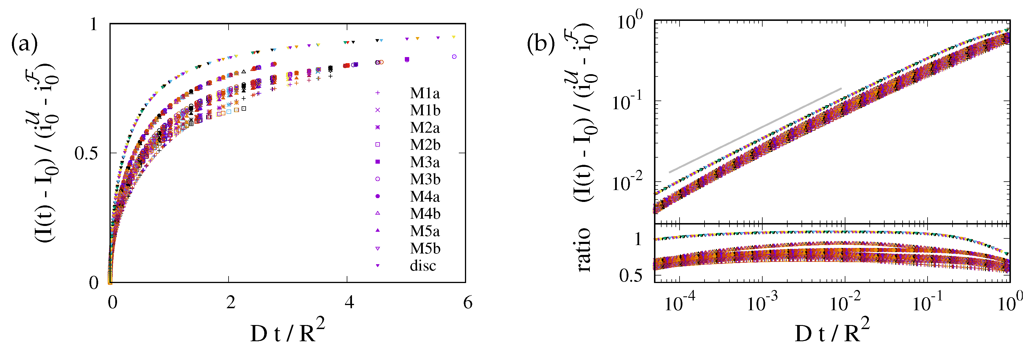
This prediction is tested in Fig. 4 where we plot data for the different geometries of the ER and for the 2D planar geometry. For each geometry the data for different diffusion coefficients collapse on a master curve. However, data for different geometries lie on distinctly different curves. The values of data for different ER geometries vary by about 20%, and those for the disk geometry (uppermost curve in the plot) take noticeably higher values. This highlights the importance of the ER geometry for the FRAP relaxation.

Figure 4. Data collapse for the reduced density $(I\left(t\right)-I\left(0\right))/\left(|i_0^{\mathcal{U}}-i_0^{\mathcal{F}}|\right)$ as function of the dimensionless time $t/R^2$. Different colors refer to different values of , that take values in $D\in \{5\times {10}^{-4}\mathsf{\mu }{\mathrm{m}}^2/\mathrm{s},1.5\times {10}^{-3}\mathsf{\mu }{\mathrm{m}}^2/\mathrm{s},\cdots ,0.1\mathsf{\mu }{\mathrm{m}}^2/\mathrm{s}\}$. The symbols refer to different geometries, as specified in the legend. (a) Simulation data with a linear scale. There are different curves for each geometry, but for any given geometry the data with different D collapse on a single line. (b) The upper panel provides a double-logarithmic plot of the data shown in (a). The lower panel shows the ratio of the data and $\sqrt{Dt/R^2}$. To a good approximation it is a horizontal line. Hence, the data lie on a power law with exponent $1/2$, where the ratio provides the prefactor of the power law. For the planar geometry the prefactor takes a value slightly larger than one. For the bicontinuous structures it differs for each geometry, with values in the rage between $0.5$ and $0.8$.

Figure 4. Data collapse for the reduced density $(I\left(t\right)-I\left(0\right))/\left(|i_0^{\mathcal{U}}-i_0^{\mathcal{F}}|\right)$ as function of the dimensionless time $t/R^2$. Different colors refer to different values of , that take values in $D\in \{5\times {10}^{-4}\mathsf{\mu }{\mathrm{m}}^2/\mathrm{s},1.5\times {10}^{-3}\mathsf{\mu }{\mathrm{m}}^2/\mathrm{s},\cdots ,0.1\mathsf{\mu }{\mathrm{m}}^2/\mathrm{s}\}$. The symbols refer to different geometries, as specified in the legend. (a) Simulation data with a linear scale. There are different curves for each geometry, but for any given geometry the data with different D collapse on a single line. (b) The upper panel provides a double-logarithmic plot of the data shown in (a). The lower panel shows the ratio of the data and $\sqrt{Dt/R^2}$. To a good approximation it is a horizontal line. Hence, the data lie on a power law with exponent $1/2$, where the ratio provides the prefactor of the power law. For the planar geometry the prefactor takes a value slightly larger than one. For the bicontinuous structures it differs for each geometry, with values in the rage between $0.5$ and $0.8$.

Figure 4 suggests that the relaxation of the reduced density has a time dependence proportional to the square root of the dimensionless time. We will show now that this is an immediate consequence of the form of the initial condition.

For the initial condition, Eq. (2), the intensity $i_{\mathrm{ns}5\mathrm{a}}(t,\mathbf{x})$ takes the form of the step function,

For early times the flow is orthogonal to the surface, i.e., curvature and topology of the surface may still be neglected. The gradient of the density therefore follows the evolution of diffusive decay of a step function in one dimension2

Right on the interface, we have $\ell =0$, and the exponential function takes the value of one. Hence, Eq. (6a) reduces to

Integrating time from $t_0=0$ till t provides

This result explains the square root dependence of the intensity observed in Fig. 4, and it provides the leading order dependence of the dependence on the surface geometry via the characteristic length scale $\Lambda =\sqrt{4\pi }\left|\mathcal{F}\right|/|\partial \mathcal{F}|$.

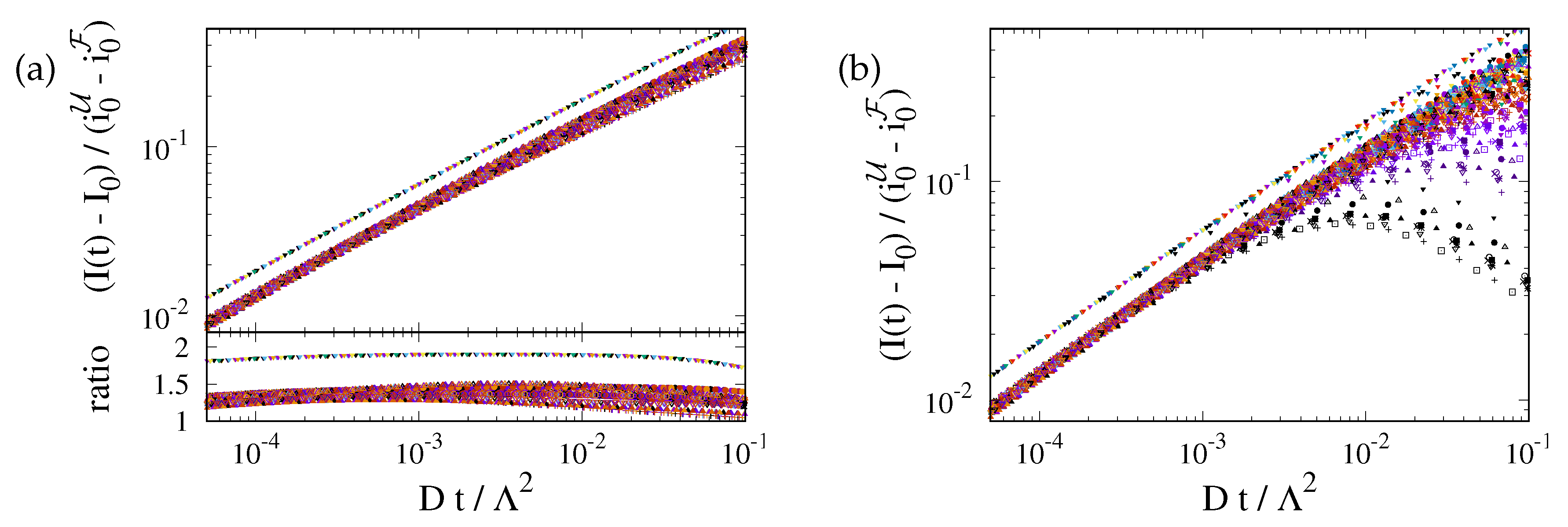
The prediction is tested in Fig. 5(a). At late time the recovery is still considerably impacted by the ER geometry. The curves for different geometries differ by up to 25%. However, at early time the transformation from a time scale $Dt/R^2$ to $Dt/{\Lambda }^2$ provides a very nice data collapse for the ER geometries. For a perfect fit the ratio of the data and $\sqrt{Dt/{\Lambda }^2}$ must be one. For our simulations it takes a value close to ${\varphi }_{-}=1.25$. We attribute this difference to the impact of the nontrivial curvature of the border of F.3

Figure 5. (a) Master plot, Eq. (9), for the data shown in Fig. 4(b). The values of $\Lambda$ depend on the geometry. This reduces the variance of the prefactors by roughly a factor of two. For the ER geometries they take values of about ${\varphi }_{-}=1.25\left(7\right)$. For a 2D disk it is close to $1.8$. (b) The same master plot for data with non-vanishing photobleaching, $r_p$. At early times the data still follow the prediction, but now there is a cross-over to a regime where photobleaching has a severe impact.

Figure 5. (a) Master plot, Eq. (9), for the data shown in Fig. 4(b). The values of $\Lambda$ depend on the geometry. This reduces the variance of the prefactors by roughly a factor of two. For the ER geometries they take values of about ${\varphi }_{-}=1.25\left(7\right)$. For a 2D disk it is close to $1.8$. (b) The same master plot for data with non-vanishing photobleaching, $r_p$. At early times the data still follow the prediction, but now there is a cross-over to a regime where photobleaching has a severe impact.

3.3. Accounting for Photobleaching

The data collapse at early times also holds for systems with bleaching (Fig. 5(b)). However, at late times these systems cross over to a decay of the intensity that is caused by bleaching. In order to gain insight into this behavior we insert Eq. (7) into Eq. (5), where K is a dimensionless constant. This equation can be integrated where erf$\left(x\right)$ is the error function. Rearranging the terms provides

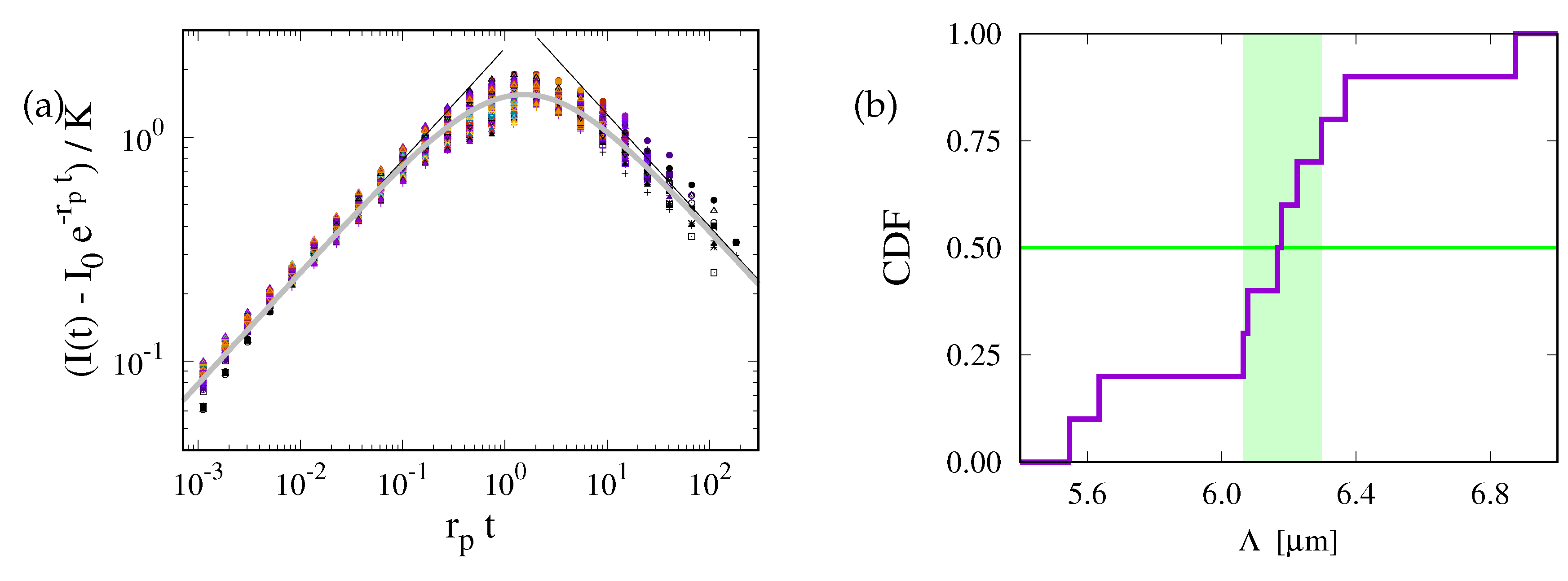
This prediction is tested in Fig. 6(a). Indeed we observe a data collapse. It features a cross over between different power laws for small and large values of $r_{p}t$.

For $r_{p}t\ll 1$ the exponential function and the error function on the right-hand side can be expanded in a power series. This entails a square-root dependence for early times,

This is in line with Fig. 6(a) where the data for small $r_{p}t$ lie close to $2{\varphi }_{-}\sqrt{r_{p}t}$ with ${\varphi }_{-}=1.25$. Here, the correction factor ${\varphi }_{-}$ accounts for the curvature effects reported in Fig. 5(a).

To find the asymptotics for $r_{p}t\gg 1$ we observe that

This is in line with the data collapse in Fig. (6a) where the data for large $r_{p}t$ lie close to $2{\varphi }_{+}/\sqrt{r_{p}t}$ with ${\varphi }_{+}=2$. Here, a correction term, ${\varphi }_{+}$, of the prefactor is expected since Eq. (7) is based on an approximation that applies only for early times.

Figure 6. (a) Data collapse of all data on a master curve predicted by Eq. (11). There is a very good collapse for small times, and the cross-over due to photobleaching is also accounted for. The two straight gray lines show the function $2{\varphi }_{-}\sqrt{r_{p}t}$ and $2{\varphi }_{+}/\sqrt{r_{p}t}$ with ${\varphi }_{-}=1.25$ and ${\varphi }_{+}=2$, respectively. An extrapolation that agrees very well with the observed data is provided by $2{\varphi }_{-}{\varphi }_{+}\sqrt{r_{p}t}/({\varphi }_{+}+{\varphi }_{-}{r}_{p}t)$ (thick solid gray line). (b) cumulative distribution of the values of $\Lambda =\sqrt{4\pi }\left|\mathcal{F}\right|/|\partial \mathcal{F}|$. For $\mathcal{F}$ with a radius of $R=3.5\mathsf{\mu }\mathrm{m}$ in the presently considered ER geometries the values of $\Lambda$ are sharply centered in a narrow interval with a width of $0.3$$\mathsf{\mu }\mathrm{m}$ (shaded region) around a median of $\overline{\Lambda }\simeq 6.17\mathsf{\mu }\mathrm{m}$.

Figure 6. (a) Data collapse of all data on a master curve predicted by Eq. (11). There is a very good collapse for small times, and the cross-over due to photobleaching is also accounted for. The two straight gray lines show the function $2{\varphi }_{-}\sqrt{r_{p}t}$ and $2{\varphi }_{+}/\sqrt{r_{p}t}$ with ${\varphi }_{-}=1.25$ and ${\varphi }_{+}=2$, respectively. An extrapolation that agrees very well with the observed data is provided by $2{\varphi }_{-}{\varphi }_{+}\sqrt{r_{p}t}/({\varphi }_{+}+{\varphi }_{-}{r}_{p}t)$ (thick solid gray line). (b) cumulative distribution of the values of $\Lambda =\sqrt{4\pi }\left|\mathcal{F}\right|/|\partial \mathcal{F}|$. For $\mathcal{F}$ with a radius of $R=3.5\mathsf{\mu }\mathrm{m}$ in the presently considered ER geometries the values of $\Lambda$ are sharply centered in a narrow interval with a width of $0.3$$\mathsf{\mu }\mathrm{m}$ (shaded region) around a median of $\overline{\Lambda }\simeq 6.17\mathsf{\mu }\mathrm{m}$.

4. Novel Approaches to analyze FRAP Data

Table 1. Comparison of estimated quench rates and diffusion coefficients for the cell lines introduced in the left and right panel of Fig. 2. The first row shows the results of Ref. [45]. The other two rows are obtained by two different approaches for the data analysis that are discussed in Sects. 4.1 and 4.2 of the present study. Their respective results are summarized in Figs. 7 and 8.

Figure 7. Fitting the diffusion constant to experimental data values. Panels (a) and (b) show data for the two cell lines introduced in Fig. 2 where the left-hand side of Eq. (13) is plotted as function of time. The solid black lines show the prediction of Eq. (9) with correction factor ${\varphi }_{-}=1.25$ when it is evaluated for the data obtained in Ref. [45]. The gray lines provide the dependences by the best fits obtained for the values of D obtained in Sect. 4.2. See Tab. 1 for a summary of these values.

Figure 7. Fitting the diffusion constant to experimental data values. Panels (a) and (b) show data for the two cell lines introduced in Fig. 2 where the left-hand side of Eq. (13) is plotted as function of time. The solid black lines show the prediction of Eq. (9) with correction factor ${\varphi }_{-}=1.25$ when it is evaluated for the data obtained in Ref. [45]. The gray lines provide the dependences by the best fits obtained for the values of D obtained in Sect. 4.2. See Tab. 1 for a summary of these values.

Figure 8. Analysis of the experimental data considered in Fig. (7) that is based on Eq. (14). Panels (a) and (b) show data for the two cell lines together with the best fits for $r_p=4\times {10}^{-3}/\mathrm{s}$ where the fit proceeds through the expectation of the distribution of data for large values of $r_{p}t$. Panels (c) and (d) show the prediction of D obtained by the analysis of the factor K. The small points with error bars refer to our present data. The points indicated by large boxes provides the value suggested in Ref. [45], and the solid line shows the extrapolation to other quench rates described in the appendix of that paper. For the quench rates obtained in the present analysis the predictions agree within the error margins.

Figure 8. Analysis of the experimental data considered in Fig. (7) that is based on Eq. (14). Panels (a) and (b) show data for the two cell lines together with the best fits for $r_p=4\times {10}^{-3}/\mathrm{s}$ where the fit proceeds through the expectation of the distribution of data for large values of $r_{p}t$. Panels (c) and (d) show the prediction of D obtained by the analysis of the factor K. The small points with error bars refer to our present data. The points indicated by large boxes provides the value suggested in Ref. [45], and the solid line shows the extrapolation to other quench rates described in the appendix of that paper. For the quench rates obtained in the present analysis the predictions agree within the error margins.

4.1. Analysis Based on Eq. (9)

The first option is to collect a vast amount of data for times where bleaching still has negligible impact. To work out this condition we expand the exponential function on the left-hand side of Eq. (12), insert the expression of K, and rearrange terms. This provides Eq. (9) and its leading order corrections

In Figs. 7(a) and (b) we plot the left-hand side of Eq. (13) as function of t. The two panels refer to the two cell lines introduced in Fig. 2. The lines with different colors show the results of repeated experiments. In view of Fig. 5(a) we expect a square-root dependence, ${\varphi }_{-}\sqrt{D/{\Lambda }^2}\sqrt{t}$. Hence, one can infer D based only on knowledge of the geometrical parameter $\Lambda$ of the measurement region — provided that one clearly resolves the power law at early times. For the first cell line this is given. For the second cell line we do not recommend this analysis. However, for the provision of the reader we provide the power laws for the values obtained in [45] and those that will be derived in Sect. 4.2 by solid black and gray lines, respectively. A direct fit of the data (if successful) provides a value of somewhere in between these two values (cf. Tab. 1).

Equation (13) entails that the corrections are small as long as

For the values of $r_p$ and D of [45] the latter factors take the values $2.5$ and $0.5$, respectively. The fit should be performed for times earlier than 50 $\mathrm{s}$ and 15 $\mathrm{s}$, respectively, when one requires that the corrections must be smaller than 5% of the leading contribution. This entails that the impact of the photobleaching in the second experiment can considerably be reduced by performing experiments with a stronger initial photobleaching, i.e. a smaller $I_0$.

In summary, this approach of data analysis can be applied when the range of data till the cutoff time spans at least one order of magnitude. The estimate of will then only rely on knowledge of the expectation of the parameter $\Lambda$, i.e. on a geometric parameter characterizing the geometry of the ER in $\mathcal{F}$. When $\left|\mathcal{F}\right|$ and $|\partial \mathcal{F}|$ are measured for some structures it can most reliably be obtained based by inspecting the cumulative distribution function of $\Lambda =\sqrt{4\pi }\left|\mathcal{F}\right|/|\partial \mathcal{F}|$, as shown in Fig. 6(b).

4.2. Analysis Based on Eq. (11)

Equation (11) provides a slightly more involved data analysis that takes into account the impact of photobleaching during the experiments. It is based on the observation of Sect. 3.3 that the data collapse of Eq. (11) can be described as a cross-over of two power laws (cf. Fig. 6)

Hence, for every given experimental data set we obtain K for a given $r_p$ by fitting $I\left(t\right)$ with the right-hand side of Eq. (14b). In view of Eqs. (10) and (8) the variability of the values of K reflects to a substantial part the different structure of the ER in the measurement region. This is reflected in the substantially improved data collapse shown in Fig. 7. In these plots we determine the preferred choice of $r_p$ by looking for the best match of the fit (solid gray line) and the expectation of the data for the largest values of $r_{p}t$. In the present case this amounts to $r_p=0.004\left(1\right)/\mathrm{s}$ for both data sets. This reflects the expectation that the quench rate is independent of the investigated cell line. It is a parameter set by the properties of the dye and the laser system of the setup. Accordingly, we find the best fits $=0.075\left(15\right)\mathsf{\mu }{\mathrm{m}}^2/\mathrm{s}$ and $=0.034\left(13\right)\mathsf{\mu }{\mathrm{m}}^2/\mathrm{s}$ for the data shown in Fig. 8(a) and (b), respectively. These regions are marked by green rectangles Fig. 8(c) and (d). The estimates for other quench rates are given by plus-symbols with error bars in those panels.

Moreover, in this figure the estimates suggested in Ref. [45] are shown by large squares. These estimates were obtained, however, for smaller values of $r_p$ because the analysis of Ref. [45] is biased to provide the quench rates that are systematically too small.4 On the other hand, Eq. (A1) and table (A5) of Ref. [45] provide a prediction of how the values of the diffusion coefficients change when adopting other values of $r_p$. It is shown by the solid lines shown in Fig. 8(c) and (d). For $r_p=0.004/\mathrm{s}$ we find $D=0.061\mathsf{\mu }{\mathrm{m}}^2/\mathrm{s}$ and $D=0.018\mathsf{\mu }{\mathrm{m}}^2/\mathrm{s}$ for the first and second cell line, respectively. These values lie at the smaller side, but still within the error margins of the present analysis. They are shown by the small squares.

We believe that the present approach of the data analysis provides a more reliable estimates of $r_p$, which is based on the bending of the lines shown in Fig. 8(a) and (b). Moreover, it explicitly accounts for the substantial correlations of the structure of the ER in the measurement region and the observed FRAP signal, while [45] adopted a Bayesian average of the different diffusion coefficients encountered when aiming for a best match of the relaxation of measurement data and simulations performed for a different ER geometry. We believe that this is the origin of the slight difference of the present estimate and the values suggested in Ref. [45].

5. Discussion and Conclusion

Abbreviations

References

1. Bakrania, S.; Chavez, C.; Ipince, A.; Rocca, M.; Oliver, S.; Stansfield, C.; Subrahmanian, R. Impacts of Pandemics and Epidemics on Child Protection: Lessons learned from a rapid review in the context of COVID-19. Technical report, UNICEF Office of Research - Innocenti, Florence, 2020.
2. World Health Organization. COVID-19 strategic preparedness and response plan: Monitoring and evaluation framework. Technical report, Geneva, 2021.
3. World Health Organization. 2021 Mid-Year Report: WHO Strategic action against COVID-19. Technical report, Geneva, 2021.
4. World Health Organization. Scoping review of interventions to maintain essential services for maternal, newborn, child and adolescent health and older people during disruptive events. Technical report, Geneva, 2021.
5. World Health Organization. Global Hepatitis Report 2017. Technical report, Geneva, 2017.
6. World Health Organization. WHO Strategic Response Plan: West Africa Ebola Outbreak. Technical report, Geneva, 2015.
7. Horvath, P.; Barrangou, R. CRISPR/Cas, the immune system of bacteria and archaea. Science 2010, 327, 167–170. [Google Scholar] [CrossRef] [PubMed]
8. Barrangou, R.; Doudna, J.A. Applications of CRISPR technologies in research and beyond. Nature Biotechnology 2016, 34, 933–941. [Google Scholar] [CrossRef] [PubMed]
9. Powell, R.; Buchanan, A. Breaking Evolution’s Chains: The Prospect of Deliberate Genetic Modification in Humans. The Journal of Medicine and Philosophy: A Forum for Bioethics and Philosophy of Medicine 2011, 36, 6–27. [Google Scholar] [CrossRef] [PubMed]
10. Baltimore, D.; Berg, P.; Botchan, M.; Carroll, D.; Charo, R.A.; Church, G.; Corn, J.E.; Daley, G.Q.; Doudna, J.A.; Fenner, M.; et al. A prudent path forward for genomic engineering and germline gene modification. Science 2015, 348, 36–38. [Google Scholar] [CrossRef] [PubMed]
11. Sinclair, A.; Islam, S.; Jones, S. Gene therapy: an overview of approved and pipeline technologies. Technical Report 171, CADTH, Ottawa, 2018.
12. Mullard, A. Gene-editing pipeline takes off. Nature Reviews Drug Discovery 2020, 19, 367–372. [Google Scholar] [CrossRef]
13. Vilchez, R.A.; Kozinetz, C.A.; Butel, J.S. Conventional epidemiology and the link between SV40 and human cancers. Lancet Oncol. 2003, 4, 188–191. [Google Scholar] [CrossRef] [PubMed]
14. Liao, J.B. Viruses and Human Cancer. Yale J Biol Med 2006, 79, 115–122. [Google Scholar] [PubMed]
15. Lambert, P.F.; Sugden, B. Viruses and Human Cancer. In Abeloff’s Clinical Oncology, 5th ed.; Niederhuber, J.E., Armitage, J.O., Dorshow, J.H., Kastan, M.B., Tepper, J.E., Eds.; Elsevier: Philadelphia, 2014. [Google Scholar]
16. Padariya, M.; Kalathiya, U.; Mikac, S.; Dziubek, K.; Fernandez, M.C.T.; Sroka, E.; Fahraeus, R.; Sznarkowska, A. Viruses, cancer and non-self recognition. Open Biol. 2021, 11, 200348. [Google Scholar] [CrossRef]
17. Miest, T.S.; Cattaneo, R. New viruses for cancer therapy: meeting clinical needs. Nature Reviews Microbiology 2014, 12, 23–34. [Google Scholar] [CrossRef]
18. Fukuhara, H.; Ino, Y.; Todo, T. Oncolytic virus therapy: A new era of cancer treatment at dawn. Cancer Science 2016, 107, 1373–1379. [Google Scholar] [CrossRef]
19. Ma, X.Y.; D. Hill, B.; Hoang, T.; Wen, F. Virus-inspired strategies for cancer therapy. Seminars in Cancer Biology 2021, in press. [Google Scholar] [CrossRef]
20. Hufnagel, L.; Brockmann, D.; Geisel, T. Forecast and control of epidemics in a globalized world. PNAS 2004, 101, 15124–15129. [Google Scholar] [CrossRef]
21. Deuffic, S.; Buffat, L.; Poynard, T.; Valleron, A.J. Modeling the hepatitis C virus epidemic in france. Hepatology 2003. [Google Scholar] [CrossRef] [PubMed]
22. Monath, T.P.; Vasconcelos, P.F. Yellow fever. Journal of Clinical Virology 2015, 64, 160–173. [Google Scholar] [CrossRef]
23. Lowe, R.; Barcellos, C.; Cruz, O.G.; Honório, N.A.; Kuper, H.; Carvalho, M.S. The Zika Virus Epidemic in Brazil: From Discovery to Future Implications. Int. J. Environ. Res. Public Health 2018, 15, 96. [Google Scholar] [CrossRef] [PubMed]
24. V’kovski, P.; Kratzel, A.; Steiner, S.; Stalder, H.; Thiel, V. Coronavirus biology and replication: implications for SARS-CoV-2. Nature Review Microbiology 2021, 19, 155–170. [Google Scholar] [CrossRef] [PubMed]
25. Targett-Adams, P.; Boulant, S.; McLauchlan, J. Visualization of double-stranded RNA in cells supporting hepatitis C virus RNA replication. J. Virol. 2008, 82, 2182–95. [Google Scholar] [CrossRef] [PubMed]
26. Romero-Brey, I.; Merz, A.; Chiramel, A.; Lee, J.Y.; Chlanda, P.; Haselman, U.; Santarella-Mellwig, R.; Habermann, A.; Hoppe, S.; Kallis, S.; et al. Three-dimensional architecture and biogenesis of membrane structures associated with hepatitis C virus replication. PLoS Path. 2012, 8, e1003056. [Google Scholar] [CrossRef] [PubMed]
27. Paul, D.; Bartenschlager, R. Architecture and biogenesis of plus-strand RNA virus replication factories. Wo. J. Vir. 2013, 2, 1–000. [Google Scholar] [CrossRef]
28. Targett-Adams, P.; Graham, E.J.; Middleton, J.; Palmer, A.; Shaw, S.M.; Lavender, H.; Brain, P.; Tran, T.D.; Jones, L.H.; Wakenhut, F.; et al. Small molecules targeting hepatitis C virus-encoded NS5A cause subcellular redistribution of their target: insights into compound modes of action. J. Virol. 2011, 85, 6353–68. [Google Scholar] [CrossRef]
29. Chukkapalli, V.; Berger, K.L.; Kelly, S.M.; Thomas, M.; Deiters, A.; Randall, G. Daclatasvir inhibits hepatitis C virus NS5A motility and hyper-accumulation of phosphoinositides. Virology 2015, 476, 168–179. [Google Scholar] [CrossRef] [PubMed]
30. Wölk, B.; Büchele, B.; Moradpour, D.; Rice, C.M. A dynamic view of hepatitis C virus replication complexes. J. Virol. 2008, 82, 10519–31. [Google Scholar] [CrossRef]
31. Eyre, N.S.; Fiches, G.N.; Aloia, A.L.; Helbig, K.J.; McCartney, E.M.; McErlean, C.S.P.; Li, K.; Aggarwal, A.; Turville, S.G.; Bearda, M.R. Dynamic imaging of the hepatitis C virus NS5A protein during a productive infection. J. Virol. 2014, 88, 3636–3652. [Google Scholar] [CrossRef] [PubMed]
32. Welsch, S.; Miller, S.; Romero-Brey, I.; Merz, A.; Bleck, C.K.; Walther, P.; Fuller, S.D.; Antony, C.; Krijnse-Locker, J.; Bartenschlager, R. Composition and three-dimensional architecture of the dengue virus replication and assembly sites. Cell Host Micr. 2009, 5, 365–75. [Google Scholar] [CrossRef] [PubMed]
33. Hoenen, T.; Biedenkopf, N.; Zielecki, F.; Jung, S.; Groseth, A.; Feldmann, H.; Becker, S. Oligomerization of Ebola Virus VP40 Is Essential for Particle Morphogenesis and Regulation of Viral Transcription. J. Virol. 2010, 84, 7053–7063. [Google Scholar] [CrossRef]
34. Hoenen, T.; Shabman, R.S.; Groseth, A.; Herwig, A.; Weber, M.; Schudt, G.; Dolnik, O.; Basler, C.F.; Becker, S.; Feldmann, H. Inclusion Bodies Are a Site of Ebolavirus Replication. J. Virol. 2012, 86, 11779–11788. [Google Scholar] [CrossRef] [PubMed]
35. Noda, T.; Ebihara, H.; Muramoto, Y.; Fujii, K.; Takada, A.; "et.al.". Assembly and budding of Ebolavirus. PLoS Pathog 2006, 2, e99. [CrossRef]
36. Stahelin, R.V. Membrane binding and bending in Ebola VP40 assembly and egress. Front. Microbiol. 2014, 5, 300. [Google Scholar] [CrossRef]
37. Bhattacharyya, S.; Hope, T.J. Full-length Ebola glycoprotein accumulates in the endoplasmic reticulum. Virol. J. 2011, 8, 11. [Google Scholar] [CrossRef] [PubMed]
38. Bharat, T.; Noda, T.; Riches, J.; Kraehling, V.; Kolesnikovac, L.; Becker, S.; Kawaok, Y.; Briggs, J.A.G. Structural dissection of Ebola virus and its assembly determinants using cryo-electron tomography. PNAS 2012, 109, 4275–4280. [Google Scholar] [CrossRef]
39. Frieman, M.; Yount, B.; Heise, M.; Kopecky-Bromberg, S.A.; Palese, P.; Baric, R.S. Severe Acute Respiratory Syndrome Coronavirus ORF6 Antagonizes STAT1 Function by Sequestering Nuclear Import Factors on the Rough Endoplasmic Reticulum/Golgi Membrane. J. Virol. 2007, 81, 9812–9824. [Google Scholar] [CrossRef]
40. Olejnik, J.; Ryabchikova, E.; Corley, R.; Mühlberger, E. Intracellular Events and Cell Fate in Filovirus Infection. Virus 2011, 3, 1501–1531. [Google Scholar] [CrossRef] [PubMed]
41. Pegoraro, G.; Bavari, S.; Panchal, R. Shedding Light on Filovirus Infection with High-Content Imaging. Virus 2012, 4, 1354–1371. [Google Scholar] [CrossRef] [PubMed]
42. Schudt, G.; Kolesnikova, L.; Dolnik, O.; Sodeik, B.; Becker, S. Live-cell imaging of Marburg virus-infected cells uncovers actin-dependent transport of nucleocapsids over long distances. PNAS 2013, 110, 14402–14407. [Google Scholar] [CrossRef] [PubMed]
43. Knodel, M.M.; Nägel, A.; Reiter, S.; Rupp, M.; Vogel, A.; Targett-Adams, P.; Herrmann, E.; Wittum, G. Multigrid analysis of spatially resolved hepatitis C virus protein simulations. Computing and Visualization in Science 2015, 17, 235–253. [Google Scholar] [CrossRef]
44. Knodel, M.M.; Reiter, S.; Targett-Adams, P.; Grillo, A.; Herrmann, E.; Wittum, G. 3D Spatially Resolved Models of the Intracellular Dynamics of the Hepatitis C Genome Replication Cycle. Viruses 2017, 9, 282. [Google Scholar] [CrossRef]
45. Knodel, M.M.; Nägel, A.; Reiter, S.; Rupp, M.; Vogel, A.; Targett-Adams, P.; McLauchlan, J.; Herrmann, E.; Wittum, G. Quantitative analysis of Hepatitis C NS5A viral protein dynamics on the ER surface. Viruses 2018, 10, 28. [Google Scholar] [CrossRef]
46. Knodel, M.M.; Nägel, A.; Reiter, S.; Rupp, M.; Vogel, A.; Lampe, M.; Targett-Adams, P.; Herrmann, E.; Wittum, G. On Estimation of a Viral Protein Diffusion Constant on the Curved Intracellular ER Surface. In Proceedings of the High Performance Computing in Science and Engineering 15: Transactions of the High Performance Computing Center, Stuttgart (HLRS) 2015; Nagel, E.W.; Kröner, H.D.; Resch, M.M., Eds., Cham, 2016; pp. 641–657. [CrossRef]
47. Knodel, M.M.; Reiter, S.; Targett-Adams, P.; Grillo, A.; Herrmann, E.; Wittum, G. Advanced Hepatitis C Virus Replication PDE Models within a Realistic Intracellular Geometric Environment. Int. J. Environ. Res. Public Health 2019, 16, 513. [Google Scholar] [CrossRef]
48. Chatel-Chaix, L.; Bartenschlager, R. Dengue virus and Hepatitis C virus-induced replication and assembly compartments: The enemy inside - caught in the web. J. Virol. 2014, 88, 5907–11. [Google Scholar] [CrossRef] [PubMed]
49. Moradpour, D.; Penin, F.; Rice, C.M. Replication of hepatitis C virus. Nat. Rev. Microbiol. 2007, 5, 453–463. [Google Scholar] [CrossRef]
50. Jones, D.M.; Gretton, S.N.; McLauchlan, J.; Targett-Adams, P. Mobility analysis of an NS5A-GFP fusion protein in cells actively replicating hepatitis C virus subgenomic RNA. J. Gen. Vir. 2007, 88, 470–5. [Google Scholar] [CrossRef]
51. Belda, O.; Targett-Adams, P. Small molecule inhibitors of the hepatitis C virus-encoded NS5A protein. Vir. Res. 2012, 170, 1–14. [Google Scholar] [CrossRef]
52. Reits, E.A.J.; Neefjes, J.J. From fixed to FRAP: measuring protein mobility and activity in living cells. Nat. Cell Biol. 2001, 3, E145–E147. [Google Scholar] [CrossRef] [PubMed]
53. Ishikawa-Ankerhold, H.C.; Ankerhold, R.; Drummen, G.P.C. Advanced Fluorescence Microscopy Techniques — FRAP, FLIP, FLAP, FRET and FLIM. Mol. 2012, 17, 4047–4132. [Google Scholar] [CrossRef]
54. Lanoiselée, Y.; Moutal, N.; Grebenkov, D. Diffusion-limited reactions in dynamic heterogeneous media. Nat Commun 2018, 9. [Google Scholar] [CrossRef]
55. Sarkar, S. Concentration Dependence of Diffusion-Limited Reaction Rates and Its Consequences. Phys. Rev. X 2020, 10, 041032. [Google Scholar] [CrossRef]
56. Fowler, A.C. Mathematical Models in the Applied Sciences; Cambridge Texts in Applied Mathematics, Cambridge UP: Cambbridge, UK, 1997. [Google Scholar]
57. Barenblatt, G.I. Scaling; Cambridge UP: Cambridge, UK, 2003. [Google Scholar]
58. Friedman, J.R.; Voeltz, G.K. The ER in 3D: a multifunctional dynamic membrane network. Tr. in Cell Biol. 2011, 21, 709. [Google Scholar] [CrossRef] [PubMed]
59. Means, S.; Smith, A.J.; Shepherd, J.; Shadid, J.; Fowler, J.; Wojcikiewicz, R.J.H.; Mazel, T.; Smith, G.D.; Wilson, B.S. Reaction diffusion modeling of calcium dynamics with realistic ER geometry. Biophysical Journal 2006, 91, 537–557. [Google Scholar] [CrossRef] [PubMed]
60. Morse, P.M.; Feshbach, H. Methods of Theoretical Physics; Vol. 1, International Series in Pure and Applied Physics, McGraw-Hill: New York, 1953.
61. Grima, R.; Schnell, S. A systematic investigation of the rate laws valid in intracellular environments. Biophysical Chemistry 2006, 124, 1–10. [Google Scholar] [CrossRef]
62. Boltz, H.H.; Sirbu, A.; Stelzer, N.; de Lanerolle, P.; Winkelmann, S.; Annibale, P. The Impact of Membrane Protein Diffusion on GPCR Signaling. Cells 2022, 11. [Google Scholar] [CrossRef]
63. Yogurtcu, O.N.; Johnson, M.E. Theory of bi-molecular association dynamics in 2D for accurate model and experimental parameterization of binding rates. J. Chem. Phys. 2015, 143, 084117. [Google Scholar] [CrossRef]