Preprint
Article

Spatio-Temporal Dual Kriging with Adaptive Coefficient Drift Function

Altmetrics

Downloads

75

Views

21

Comments

0

A peer-reviewed article of this preprint also exists.

Submitted:

05 January 2024

Posted:

08 January 2024

You are already at the latest version

Alerts
Abstract
Research on spatio-temporal geostatistical modelling remains a critical challenge in numerous scientific and engineering disciplines. This work introduces a novel extension of the dual kriging the spatio-temporal dual kriging (ST-DK) whose drift functions with fixed and adaptive coefficients are established. The approach appears to be effective in modelling complex spatio-temporal dynamics, particularly when relevant auxiliary variables exert substantial influence on the target variable. To illustrate its performance, we compare the ST-DK model with the classical spatio-temporal regression kriging (ST-RK) method for estimating temperature and air pressure data across Thailand in 2018. Our findings demonstrate that both ST-DK and ST-RK models, when utilizing adaptive coefficients, outperform their constant coefficient counterparts. Furthermore, the ST-DK method consistently exhibits superior performance compared to the ST-RK model.
Keywords: 
Subject: Computer Science and Mathematics  -   Applied Mathematics

1. Introduction

Spatio-temporal interpolation is a computational technique that estimates the value of an interested variable at a given location and time, provided available information in the sample at other locations and times. It is a combination of spatial interpolation, which deals with the estimation of values in geographic space, and temporal interpolation, which focuses on estimating values over a specific time period. A fundamental assumption that underlies spatio-temporal interpolation is that close observations exhibit greater similarity than distant ones [1]. Spatio-temporal interpolation methods can be categorized into two distinct approaches: the reduction approach and the extension approach [2,3,4]. Within the reduction approach, time is considered an independent dimension distinct from the spatial dimensions. This methodology is a two-step process in which data are first interpolated in space at each time step, and the resulting time series at each spatial location is subsequently interpolated. In contrast, the extension approach is formulated to interpolate simultaneously in both spatial and time dimensions. The reduction methods, such as shape function-based methods, inverse distance weighted (IDW), tension spline, and global polynomial interpolations, offer a simpler and less computationally demanding procedure. However, their suitability may be limited in scenarios where the temporal component of the data plays a significant role [5,6]. On the contrary, the extension methods, such as parallel IDW, random forests, and spatio-temporal kriging methods, are more complex and computationally intensive but possess enhanced capabilities for handling situations where the temporal component is substantial and can potentially yield higher accuracy, particularly in cases where the spatio-temporal relationships are complex [7].
Spatio-temporal kriging methodologies have emerged as powerful and effective geostatistical tools applied in several fields, including environmental sciences [8], pollution demography [9], and meteorology [10,11,12]. These methods expand upon spatial kriging techniques by incorporating both spatial and temporal information and enabling the construction of an optimal linear estimator that minimizes estimation variance under the constraint of unbiasedness. This estimator is a linear combination of spatio-temporal observed values and their corresponding weights. The two most commonly employed kriging techniques in the spatio-temporal domain are spatio-temporal simple kriging (ST-SK) and spatio-temporal ordinary kriging (ST-OK). These methods do not utilize any additional information or auxiliary variables during the estimation process. Their weights are determined by the covariance function or the variogram, which is dependent on the assumed degree of stationarity ascribed to the underlying random function. The ST-SK technique assumes second-order stationarity in the random function, characterized by a constant and known mean and a known covariance function that is dependent only on the separation vector between a pair of measured points in space and time. The ST-OK method, on the other hand, necessitates the assumption of intrinsic stationarity in the random function. This implies that the mean of the random function is constant and the variance of the difference is the same between the random function at two geographic locations lagged by the same distance [13,14].
An alternative spatio-temporal kriging incorporates additional variables, referred to as auxiliary variables, into the kriging model to enhance its predictive abilities, particularly when integrating relevant auxiliary variables that influence the target variable. The spatio-temporal regression kriging (ST-RK) technique involves decomposing the target variable into two distinct components: a deterministic trend component and a stochastic residual component [8]. The trend component encapsulates the systematic variation in the target variable, which can be modeled using auxiliary variables. Conversely, the residual component represents the remaining unexplained variability, which can be modelled using either ST-OK or ST-SK. Similar to the ST-RK method, the target variable in the spatio-temporal kriging with external drift (ST-KED) process can be divided into deterministic drift and stochastic residual terms. However, unlike the ST-RK method, the ST-KED weights are directly derived from the kriging equations, which are formulated under the unbiasedness and minimum error variance conditions [15].
In recent years, these two techniques have been successfully applied in diverse applications. The ST-RK method was used to predict chlorophyll-a [8], nitrogen dioxide ( NO 2 ) concentrations [9], rainfall [10], and mean daily temperature [11]. Whereas, the ST-KED modeling technique was employed to interpolate soil water content [16], rainfall data [17], daily precipitation, and temperature [18]. Furthermore, extensive research has consistently shown that ST-KED outperforms ST-OK in terms of prediction accuracy and reliability [16,17,18]. Notwithstanding its superior performance, the ST-KED method is impeded by its computational complexity. Therefore, this study aims to tackle this limitation by developing an efficient algorithm for the ST-KED, thereby enhancing its applicability in broader practical scenarios.
In the context of spatial kriging methods, kriging with external drift (KED) is computationally expensive because it requires solving a new kriging system to determine the weights of the linear estimator for each interpolated point. In contrast, dual kriging (DK), a technique derived from KED, provides a unified approach to determining the weights of the estimator for all estimated points. Hence, DK is an advancement of KED that alleviates its computational challenges [19,20]. Although KED and DK produce the same estimated values, there is currently a dearth of research on spatio-temporal interpolation.
Motivated by this observation, we introduce a spatio-temporal dual kriging (ST-DK) algorithm to mitigate the computational burden of the ST-KED method by expanding upon the principles of spatial KED interpolation. The proposed ST-DK algorithm is designed to accommodate both fixed and adaptive coefficients of drift functions.
The remainder of this paper is structured as follows: Section 2 provides background information on ST-RK and ST-KED. Section 3 describes the construction of the proposed ST-DK methodology for fixed and adaptive coefficients of trend functions. In Section 4, a detailed description of the data and the selection criteria for auxiliary variables are presented. Subsequently, an evaluation of the proposed ST-DK method’s performance is conducted using meteorological data, including temperature and air pressure measurements. This evaluation then draws comparisons between the performance of the ST-DK method and the ST-RK method. Conclusions and discussions are drawn in Section 5.

2. Methodological Framework of Spatio-Temporal Kriging Incorporating Auxiliary Variables

Suppose that { Z ( s , t ) , ( s , t ) D × T } is a real-value stochastic process or random function on the space-time domain D × T , where D R d and T R or Z . The random variable Z ( s , t ) can be disaggregated into two components [21,22]:
Z ( s , t ) = μ ( s , t ) + ϵ ( s , t ) ,
where μ ( s , t ) denotes the deterministic drift function, also known as the trend function, while ϵ ( s , t ) is a stochastic residual with a mean of zero.
The drift function can typically be represented as a linear combination of the functions evaluated at a spatio-temporal point ( s , t ) , as expressed by the following equation [10,22,23]:
μ ( s , t ) = l = 0 L α l f l ( X ( s , t ) ) ,
where X ( s , t ) = X 1 ( s , t ) , . . . , X η ( s , t ) T is the vector of η auxiliary variables at point ( s , t ) and α l is a non-zero constant coefficient of a known deterministic function f l , which is represented in terms of auxiliary variables for l = 0 , 1 , . . . , L . The function f l is often referred to as a basis function in certain studies [24,25,26].
Given the assumption of second-order stationarity for the residual, the spatio-temporal covariance function C ( h s , h t ) exists. This covariance function quantifies the dependence between any pair of residuals separated by a spatial lag h s and temporal lag h t , defined as follows [27]:
C ( h s , h t ) = Cov ϵ ( s + h s , t + h t ) , ϵ ( s , t ) ,
where ( s + h s , t + h t ) , ( s , t ) D × T . Furthermore, the spatio-temporal variogram of the residual is given by:
γ ( h s , h t ) = 1 2 Var ϵ ( s + h s , t + h t ) ϵ ( s , t ) , = 1 2 E ϵ ( s + h s , t + h t ) ϵ ( s , t ) 2 ,
which results in
C ( h s , h t ) = C ( 0 , 0 ) γ ( h s , h t ) ,
where C ( 0 , 0 ) is the global sill value of spatio-temporal variogram.
The classical empirical spatio-temporal variogram estimator [28], which estimates the theoretical spatio-temporal variogram function (presented in Equation (4)), can be formally defined as:
γ * ( h s , h t ) = 1 2 N s ( h s ) N t ( h t ) s i , s u N s ( h s ) t j , t v N t ( h t ) ϵ ( s i , t j ) ϵ ( s u , t v ) 2 ,
where N s ( h s ) represents the set of all spatial location pairs separated by the spatial lag vector h s and N t ( h t ) denotes the set of all time point pairs separated by the temporal lag h t . The sizes of these sets, N s ( h s ) and N t ( h t ) , indicate the number of distinct pairs in each set.
Several spatio-temporal covariance models have been proposed in the literature, including the sum model [29], the metric model [30], and the product model [27]. The present study focuses on the product-sum model, which is expressed as follows [31]:
C ( h s , h t ) = k 1 C s ( h s ) C t ( h t ) + k 2 C s ( h s ) + k 3 C t ( h t ) ,
where C s and C t are spatial and temporal covariance functions, respectively. The spatial and temporal covariance functions are defined as
C s ( h s ) = C ( h s , 0 ) = C s ( 0 ) γ s ( h s ) ,
C t ( h t ) = C ( 0 , h t ) = C t ( 0 ) γ t ( h t ) ,
where C s ( 0 ) and C t ( 0 ) are the values of sill of the spatial variogram, γ s , and temporal variogram, γ t , respectively. This study uses the exponential model [32], a parametric variogram, to represent both the spatial and temporal variograms, which are fit to the corresponding empirical variograms by weighted least squares [33].
Based on the relationship between the covariance function and variogram established in Equation (5), (7) - (9), the spatio-temporal variogram can be expressed as:
γ ( h s , h t ) = [ k 1 C t ( 0 ) + k 2 ] γ s ( h s ) + [ k 1 C s ( 0 ) + k 3 ] γ t ( h t ) k 1 γ s ( h s ) γ t ( h t ) ,
where
k 1 = C s ( 0 ) + C t ( 0 ) C ( 0 , 0 ) C s ( 0 ) C t ( 0 ) , k 2 = C ( 0 , 0 ) C t ( 0 ) C s ( 0 ) , k 3 = C ( 0 , 0 ) C s ( 0 ) C t ( 0 ) .
The parameters of the spatio-temporal variogram model can be determined by fitting the empirical variogram provided in Equation (7). Subsequently, the spatio-temporal covariance function of residuals is derived by leveraging the relationship between the variogram and covariance function as provided in Equation (5).
The objective of the spatio-temporal kriging with drift function is to estimate the value of the target variable at an unobserved spatio-temporal point ( s 0 , t 0 ) , represented as Z ( s 0 , t 0 ) , where s 0 D and t 0 T . The estimation is achieved using the principles of unbiasedness and minimum error variance. Two classical spatio-temporal kriging methods, spatio-temporal regression kriging (ST-RK) and spatio-temporal kriging with external drift (ST-KED), are covered in detail in the following.

2.1. Spatio-Temporal Regression Kriging

The ST-RK estimator briefly described in the previous section consists of drift function and residual components, in which the implementation of each term is obtained independently. The drift function is conventionally modeled using multiple linear regression (MLR), while the residuals are interpolated using spatio-temporal simple kriging (ST-SK). Given a set of n × m observed values of the target variables and auxiliary variables at distinct spatio-temporal points ( s 1 , t 1 ) , . . . , ( s n , t m ) , the ST-RK estimator at the point ( s 0 , t 0 ) denoted as Z ST - RK ( s 0 , t 0 ) , can be written as [23]:
Z ST - RK ( s 0 , t 0 ) = μ ( s 0 , t 0 ) + ϵ ST - SK ( s 0 , t 0 ) , = l = 0 L α l f l ( X ( s 0 , t 0 ) ) + j = 1 m i = 1 n λ i j ϵ 0 ϵ ( s i , t j ) , = α T F 0 + ϵ T Λ ϵ 0 ,
where α = α 0 , . . . , α L T is a vector of coefficients,
F 0 = f 0 ( X ( s 0 , t 0 ) ) , . . . , f L ( X ( s 0 , t 0 ) ) T is a vector of the basis functions,
ϵ = ϵ ( s 1 , t 1 ) , . . . , ϵ ( s n , t m ) T is a residual vector, and
Λ ϵ 0 = λ 11 ϵ 0 , . . . , λ n m ϵ 0 T is the ST-SK weight vector.
The optimal weight vector for the ST-SK method is determined by minimizing the prediction error variance under the constraint of unbiasedness. This minimization problem is solved utilizing the Lagrange multiplier method, resulting in a system of linear equations known as the ST-SK system [34]:
j = 1 m i = 1 n λ i j ϵ 0 C s u s i , t v t j = C s u s 0 , t v t 0 , f o r u = 1 , . . . , n and v = 1 , . . . , m .
The ST-SK equations can be expressed in the following matrix form:
Ω Λ ϵ 0 = Ω 0 ,
where Ω = C s 1 s 1 , t 1 t 1 C s 1 s n , t 1 t m C s n s 1 , t m t 1 C s n s n , t m t m and
    Ω 0 = C s 1 s 0 , t 1 t 0 C s n s 0 , t m t 0 .

2.2. Spatio-Temporal Kriging with External Drift

Let Z ST - KED ( s 0 , t 0 ) be the estimated value of the target variable at the point ( s 0 , t 0 ) . The ST-KED estimator is expressed as a linear combination of input data, Z ( s i , t j ) for i = 1 , . . . , n and j = 1 , . . . , m [34]:
Z ST - KED ( s 0 , t 0 ) = j = 1 m i = 1 n λ i j Z ( s i , t j ) ,
= Z T Λ ,
where Z = Z ( s 1 , t 1 ) , . . . , Z ( s n , t m ) T is the vector of observed data for target variable and
Λ = λ 11 , . . . , λ n m T is the ST-KED weight vector.
The optimal weight vector for the ST-KED technique can be found using the Lagrange multiplier method to minimize the prediction error variance while satisfying the unbiasedness constraint. This approach is based on the ST-KED estimator and the form of the target variable Z, as represented by Equation (1). The ST-KED system is written as [15]:
Ω | F + F T | 0 L + 1 Λ N = Ω 0 F 0 ,
where 0 L + 1 is the ( L + 1 ) × ( L + 1 ) zero matrix,
N = η 0 , . . . , η L T represents the vector of Lagrange multipliers,
F = F 1 F m , and
F j = f 0 ( X ( s 1 , t j ) ) f L ( X ( s 1 , t j ) ) f 0 ( X ( s n , t j ) ) f L ( X ( s n , t j ) ) , for j = 1 , . . . , m .
Since the ST-KED weights need to be recalculated for each unobserved data point, this leads to a significant increase in computational resources. Employing a single weight matrix to estimate the target variable across all ungauged locations can effectively address this challenge. The spatio-temporal dual kriging (ST-DK) method is therefore proposed to overcome this limitation.

3. Methodology of Spatio-Temporal Dual Kriging

The formulation of the ST-DK interpolation is inspired by the principles of the DK [35]. The ST-DK algorithm can be described as a refinement of the ST-KED method, in which the ST-DK weight coefficient matrix is performed only once for every unobserved site. In this section, the derivation of both fixed and adaptive coefficients of the ST-DK estimation is presented. To simplify subsequent references, we will use the abbreviations FST-DK and AST-DK to designate the ST-DK method with a fixed coefficient drift function and the ST-DK method with an adaptive coefficient drift function, respectively.

3.1. Spatio-Temporal Dual Kriging with Fixed Coefficient Drift Function

Given the ST-KED system represented by Equation (16), where the coefficient matrix is assumed to be invertible, the solution can be expressed in the following form [35,36]:
Λ N = U | V + V T | W Ω 0 F 0 ,
where U , V , and W are matrices with dimensions of n m × n m , n m × ( L + 1 ) , and ( L + 1 ) × ( L + 1 ) , respectively. Substituting the weight solution of Equation (17) for the weight vector Λ in Equation (15) yields the following expression for the estimated value:
Z ST - KED ( s 0 , t 0 ) = Z T VF 0 + Z T U Ω 0 .
To establish a formal representation of the dual formulation of ST-KED, two matrices are introduced
a T = a 0 , . . . , a L = Z T V and b T = b 11 , . . . , b n m = Z T U .
Consequently, Equation (18) undergoes a transformation, resulting in a novel form known as the FST-DK estimator, as depicted below:
Z FST - DK ( s 0 , t 0 ) = l = 0 L a l f l ( X ( s 0 , t 0 ) ) + j = 1 m i = 1 n b i j C s i s 0 , t j t 0 , = a T F 0 + b T Ω 0 .
As a result, the vectors a and b become the weight vectors of the FST-DK estimator, exhibiting invariance with respect to the target point ( s 0 , t 0 ) . According to Equation (19), the weight vectors a and b can be represented in matrix form as:
b a = U | A + V T | B Z 0 ̲ L + 1 ,
where A , B are arbitrary matrices with dimensions of n m × ( L + 1 ) and ( L + 1 ) × ( L + 1 ) , respectively, and 0 ̲ L + 1 represents the zero vector of size L + 1 .
Given the substitutions A = V and B = W , the vectors of coefficients a and b are solutions of the FST-DK system,
Ω | F + F T | 0 L + 1 b a = Z 0 ̲ L + 1 .
The estimated value of the target variable at the unobserved point ( s 0 , t 0 ) is therefore obtained by substituting the vectors a and b into Equation (20).

3.2. Spatio-Temporal Dual Kriging with Adaptive Coefficient Drift Function

In the previous case, the coefficient α l , where l = 0 , 1 , . . . , L , of the drift function μ ( s , t ) in Equation (2) remain constant across all time steps. This property of the coefficients makes it simple to use in practice, as it does not require us to keep track of its value at each time step. Although this can be a significant advantage, especially when dealing with large datasets, but it is a trade-off between the estimation accuracy and a reduction in computational cost. To address this limitation and incorporate a more flexible drift function, this study proposes a novel drift function approach that incorporates dynamically adjusted coefficients. The proposed drift function, denoted by μ A , is hereby introduced as follows:
μ A ( s , t ) = l = 0 L τ = t 1 t m α l τ f l τ ( X ( s , t ) ) ,
where f l τ is l-th basis function of auxiliary variables at time step τ with α l τ R { 0 } being the constant coefficient. Furthermore, t 1 and t m represent the initial and final time steps, respectively.
For l = 0 , 1 , . . . , L , function f l τ is represented in term of auxiliary variables and is defined by the equation:
f l τ ( X ( s , t ) ) = f l ( X ( s , t ) ) , τ = t , 0 , τ t .
This expression of f l τ indicates that the drift function μ A can change over time step τ .
Incorporating these adaptive coefficients into the drift function of the ST-KED, the value at the target point ( s 0 , t 0 ) is estimated using the ST-KED estimator, as presented in Equation (14). This estimator is denoted as Z ^ ST - KED ( s 0 , t 0 ) . Moreover, the matrix equation that arises from employing the Lagrange multiplier method to minimize the variance of prediction error under the constraint of unbiasedness is expressed as follows (Refer to Appendix A for a detailed explanation of the derivation process):
Ω | F + F T | 0 ( L + 1 ) m Λ N = Ω 0 F 0 ,
where N = η 0 t 1 , . . . , η L t m T is a vector of the Lagrange multiplier,
F = F 1 0 n × ( L + 1 ) 0 n × ( L + 1 ) 0 n × ( L + 1 ) F 2 0 n × ( L + 1 ) 0 n × ( L + 1 ) 0 n × ( L + 1 ) F m ,
0 n × ( L + 1 ) represents the n × ( L + 1 ) zero matrix, and
F 0 = f 0 t 1 ( X s 0 , t 0 ) f L t m ( X s 0 , t 0 ) , see detail in Appendix A.
By applying the same procedure as in SubSection 2.2 and SubSection 3.1, the AST-DK estimator takes the following form:
Z AST - DK ( s 0 , t 0 ) = l = 0 L τ = t 1 t m a l τ f l τ ( X ( s 0 , t 0 ) ) + j = 1 m i = 1 n b i j C s i s 0 , t j t 0 , = a ^ T F 0 + b T Ω 0 ,
where a ^ and b are the vector of coefficients such that a ^ T = a 0 t 1 , . . . , a L t m and b T = b 11 , . . . , b n m .
Analogously to the approach outlined in SubSection 3.1, we can derive the AST-DK system for determining the vectors a ^ and b , which is given by
Ω | F + F T | 0 ( L + 1 ) m b a ^ = Z 0 ̲ ( L + 1 ) m .
To evaluate the effectiveness of the proposed AST-DK techniques, these methods are applied in the subsequent section to interpolate meteorological data, encompassing temperature and air pressure. Additionally, the performance of these methods will be compared to that of the ST-RK with fixed coefficient drift function (denoted as FST-RK) and the ST-RK with adaptive coefficient drift function method (denoted as AST-RK).

4. Application of the Proposed ST-DK Techniques for Temperature and Air Pressure Interpolations in Thailand

4.1. Study Area and Data Description

Our domain of study covers the entire country of Thailand, which lies between 5 37 N and 20 27 N latitude and 97 22 E and 105 37 E longitude. The total area of the country is 513,115 square kilometres, with a coastline of 3,219 kilometres [37,38]. The present study leverages observational data from the Hydro-Informatics Institute (HII) [39] including temperature (in °C), air pressure (in hPa), relative humidity (in %RH), and the Digital Elevation Model (DEM) (in metre). A comprehensive network of 226 weather stations encloses the study area, as depicted in Figure 1. The performances of the kriging schemes are evaluated based on monthly mean data over the period of January 2018 to December 2018. Prior to the interpolation process, data cleaning and preprocessing procedures are conducted to ensure data quality.

4.2. Selection of Auxiliary Variables

The estimation accuracy of both the ST-RK and ST-DK methods mainly depends on the careful selection of auxiliary variables for which a strong correlation with target variables is found [40]. This stage involves an interaction assessment between external factors and target variables using the Pearson correlation coefficient [41]. If the absolute value of the correlation coefficient exceeds a predefined threshold of 0.5 (as established in [42]), the candidate variable is considered statistically significant and deemed suitable to include in the basis functions of the drift terms. In this work, air pressure, relative humidity, and DEM are considered potential auxiliary variables for the temperature interpolation, whereas temperature, relative humidity, and DEM are those of the air pressure estimation.

4.3. Accuracy Assessment

A comparison of the performances between the proposed ST-DK and the traditional ST-RK methods is demonstrated in the case of the fixed and adaptive coefficient drift functions. The accuracy of all algorithms is evaluated using a 10 folds cross validation technique. The process is done by dividing the entire dataset into ten equal-sized folds. Each fold is then used once as the test set, while the remaining 9 folds serve as the training set [43]. After each of the 10 folds was once the left-out fold, the overall accuracy was computed by averaging prediction error values obtained from test folds. The root mean square error (RMSE) [44] and mean absolute percentage error (MAPE) [45] are the performance evaluation statistics, which can be written as follows:
RMSE = 1 N n = 1 N Z n Z n * 2
and
MAPE = 1 N n = 1 N | Z n Z n * | Z n × 100 ,
where N is the number of the observed data in each fold and Z n and Z n * are the n-th actual and estimated values, respectively.

4.4. Results

4.4.1. Comparison of ST-RK and ST-DK with Fixed Coefficient Drift Function

Table 1 presents the correlation coefficients between the target and potential auxiliary variables. It is found that air pressure is correlated with temperature more significantly than others, with the correlation coefficients being 0.5775. On the other hand, a significant negative correlation is also observed between air pressure and DEM. Consequently, air pressure and temperature are selected as each other’s auxiliary variables, with DEM being another auxiliary variable for air pressure estimation.
The drift function used in the temperature estimation process takes the following form:
μ ( s , t ) = α 0 + α 1 X 1 ( s , t ) ,
where X 1 ( s , t ) is the air pressure at point ( s , t ) . By comparing the given form with Equation (2), we observe that f 0 ( X 1 ( s , t ) ) = 1 and f 1 ( X 1 ( s , t ) ) = X 1 ( s , t ) for all point ( s , t ) . The drift function for air pressure estimation is represented by
μ ( s , t ) = α 0 + α 1 X 2 ( s , t ) + α 2 X 3 ( s , t ) ,
where X 2 ( s , t ) and X 3 ( s , t ) denote temperature and DEM at point ( s , t ) , respectively. Suppose that X ( s , t ) = X 2 ( s , t ) , X 3 ( s , t ) T and through a direct comparison with Equation (2), it follows that f 0 ( X ( s , t ) ) = 1 , f 1 ( X ( s , t ) ) = X 2 ( s , t ) , and f 2 ( X ( s , t ) ) = X 3 ( s , t ) . All unknown parameters of the drift functions are estimated through ordinary least squares (OLS) [46].
The RMSE and MAPE values attained from the FST-RK and FST-DK methods are summarized in Table 2. Regarding accuracy measures, the FST-RK exhibited superior performance in temperature estimation compared to the FST-DK. The FST-RK method reduces the RMSE and MAPE by 2.582% and 2.025%, respectively. On the contrary, the FST-DK excelled in air pressure estimation, achieving lower RMSE (15.6068%) and MAPE (4.4717%) compared to the benchmark scheme.

4.4.2. Comparison of the ST-RK and ST-DK with Adaptive Coefficient Drift Function

Since trends are assumed to be changing across time in the present case, the procedure to compute overall correlation coefficients therefore differs from the fixed coefficients case. Here, monthly correlation coefficients between variables are averaged to obtain an overall correlation. A highly positive correlated relationship is marked between temperature and air pressure, with a correlation coefficient exceeding 0.8. The DEM variable is also included in the drift function for both temperature and air pressure estimations as the absolute values of correlation coefficients are greater than 0.5.
Table 3. Monthly means of Pearson correlation coefficients between candidate auxiliary and target variables.
Variable Temperature Air Pressure
Temperature 1.0000 0.8021
Air Pressure 0.8021 1.0000
Relative Humidity -0.0710 0.3432
DEM -0.5907 -0.7608
Therefore, we define the drift function based on the selected auxiliary variables for temperature estimation. In this work, we define two such functions below, utilizing the variable definitions stated in the previous subsection. The first function is formulated as:
μ A ( s , t ) = τ = 1 12 α 0 τ f 0 τ ( X 1 ( s , t ) ) + τ = 1 12 α 1 τ f 1 τ ( X 1 ( s , t ) ) ,
where f 0 τ ( X 1 ( s , t ) ) = 1 , τ = t , 0 , τ t and
   f 1 τ ( X 1 ( s , t ) ) = X 1 ( s , t ) , τ = t , 0 , τ t
for t = 1 , 2 , . . . , 12 .
Furthermore, suppose that X ( s , t ) = X 1 ( s , t ) , X 3 ( s , t ) T , a second drift function is expressed as:
μ A ( s , t ) = τ = 1 12 α 0 τ f 0 τ ( X ( s , t ) ) + τ = 1 12 α 1 τ f 1 τ ( X ( s , t ) ) + τ = 1 12 α 2 τ f 2 τ ( X ( s , t ) ) ,
where f 0 τ ( X ( s , t ) ) = 1 , τ = t , 0 , τ t ,
   f 1 τ ( X ( s , t ) ) = X 1 ( s , t ) , τ = t , 0 , τ t , and
   f 2 τ ( X ( s , t ) ) = X 3 ( s , t ) , τ = t , 0 , τ t ,
for t = 1 , 2 , . . . , 12 .
For air pressure estimation, the drift function is formulated as:
μ A ( s , t ) = τ = 1 12 α 0 τ f 0 τ ( X ( s , t ) ) + τ = 1 12 α 1 τ f 1 τ ( X ( s , t ) ) + τ = 1 12 α 2 τ f 2 τ ( X ( s , t ) ) ,
where f 0 τ ( X ( s , t ) ) = 1 , τ = t , 0 , τ t ,
   f 1 τ ( X ( s , t ) ) = X 2 ( s , t ) , τ = t , 0 , τ t , and
   f 2 τ ( X ( s , t ) ) = X 3 ( s , t ) , τ = t , 0 , τ t ,
for t = 1 , 2 , . . . , 12 .
At each monthly time step, the unknown coefficients are identified through the application of the OLS method, as in the previous subsection.
Table 4 demonstrates the estimation performances of the AST-RK and AST-DK methods for temperature and air pressure based on the drift functions given in Equations (30)-(32). As evidenced by the RMSE and MAPE metrics, the AST-DK method with one and two auxiliary variables consistently outperform the AST-RK method for estimation of both target variables. In particular, the RMSE values attained from the AST-DK method with two auxiliary variables are 0.8336 for temperature and 10.5835 for air pressure, resulting in 12.5544% and 7.4256% improvement compared to the AST-RK method. Furthermore, the AST-RK and AST-DK methods with one auxiliary variable surpass the accuracy of the fixed-coefficient approaches presented in Table 2.
Besides, the role of the adaptive coefficient drift function in the ST-DK method becomes apparent when considering temperature estimation with a single auxiliary variable. In the case of fixed coefficients, the ST-RK model yields higher accuracy estimates than the ST-DK, but the opposite scenario occurs for the adaptive coefficient schemes.
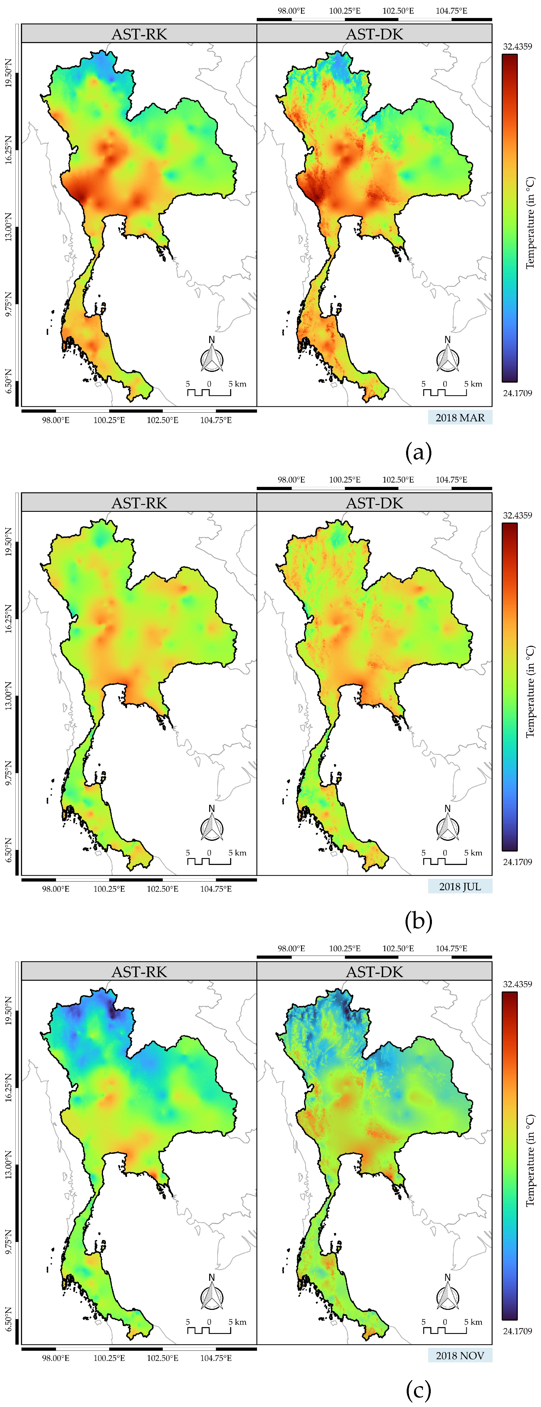
For illustration purposes, the spatial distribution maps of temperature and air pressure obtained from the AST-RK and AST-DK models are generated. The maps were gridded at a resolution of 0.05 degrees, corresponding to an approximate spatial area of 5.5 k m 2 per grid cell. Thailand’s weather is divided into mainly three seasons; the summer season (March to May), the rainy season (May to October), and the winter season (November to February) [47,48]. One month of each season (March, July, and November) was performed to represent seasonal meteorological fluctuations across the country. The temperature variations across Thailand are visualized in Figure 2. As can be seen in the figures, stronger temperature gradients are produced by the ST-DK method for all three representative months. A more dispersed distribution of high temperatures can be markedly observed in March from the north to the centre regions, as displayed in Figure 2(a).
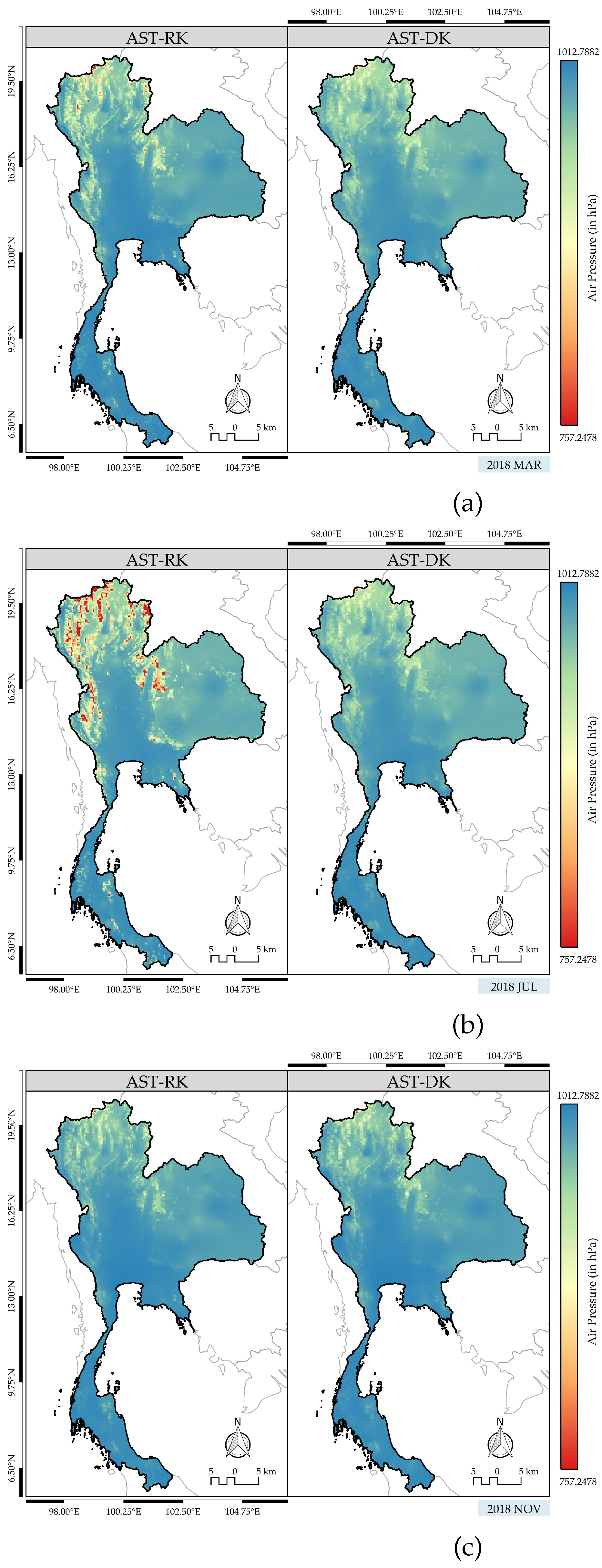
A comparison of air pressure distributions obtained from the AST-RK and AST-DK methods is presented in Figure 3. The results of both methods show similar distribution patterns for March and November. A notable difference can be found in July, in which a relatively low air pressure produced by the AST-RK model is identified in the northern area as opposed to the AST-DK approach.

5. Conclusions and Discussions

This work introduces the ST-DK technique, a novel methodological approach designed as a computationally efficient alternative to the ST-KED method for spatio-temporal interpolation. The ST-DK leverages the ability to utilize fixed coefficients within its drift functions while offering increased flexibility to incorporate adaptive coefficients. This capability enables the ST-DK to effectively model complex spatio-temporal dynamics. The results of the case study revealed that the ST-DK and ST-RK methods with adaptive coefficient drift functions demonstrated superior performance in the estimation of both temperature and air pressure compared to their counterparts employing fixed coefficients. Furthermore, the ST-DK method consistently outperformed the ST-RK method for both temperature and air pressure estimations. The advantages of the ST-DK model in estimation over the ST-RK method may be attributed to the fact that correlated residuals are considered in the DK trend process, which is not the case for the RK model. Despite the satisfactory results of this study, higher computational resources for a large number of unobserved locations and estimated time steps can be a challenge. To handle the issue of the growing dimensionality of the ST-DK system, specialized solvers designed for large linear systems are used to exploit the sparsity and symmetry of the ST-DK coefficient matrix [49,50,51]. Another practical way to boost simulation efficiency is by localizing ST-DK computations to a neighborhood of each unobserved site, resulting in a model size reduction. Possible future research endeavors include the identification of an optimal drift function and the development of techniques for determining the optimal coefficients within adaptive-coefficient drift functions tailored for the ST-DK framework.

Author Contributions

Conceptualization, C.K., N.C. and S.M.; methodology, C.K., N.C. and S.M.; software, C.K. and S.M.; validation, C.K., N.C. and S.M.; formal analysis, C.K., N.C., and S.M.; investigation, C.K., N.C. and S.M.; resources, C.K., N.C. and S.M.; data curation, C.K. and S.M.; writing-original draft preparation, C.K., N.C. and S.M.; writing-review and editing, C.K., N.C. and S.M.; visualization, C.K.; supervision, N.C. and S.M. All authors have read and agreed to the published version of the manuscript.

Funding

This work was funded by Fundamental Fund 2024, Chiang Mai University.

Data Availability Statement

All data were acquired from the National Hydroinformatics and Climate Data Center (NHC), developed by Hydro-Informatics Institute (HII) [39].

Acknowledgments

This research project was supported by (i) Chiang Mai University, (ii) Fundamental Fund, Chiang Mai University and (iii) Centre of Excellence in Mathematics, Ministry of Higher Education, Science, Research and Innovation, Thailand.

Conflicts of Interest

The authors declare no conflict of interest.

Abbreviations

The following abbreviations are used in this manuscript:
AST-DK Spatio-temporal dual kriging with adaptive coefficient drift function
AST-RK Spatio-temporal regression kriging with adaptive coefficient drift function
FST-DK Spatio-temporal dual kriging with fixed coefficient drift function
FST-RK Spatio-temporal regression kriging with fixed coefficient drift function
DEM Digital Elevation Model
DK Dual kriging
IDW Inverse distance weighted
KED Kriging with external drift
MAPE Mean absolute percentage error
MLR Multiple linear regression
NO 2 Nitrogen dioxide
OLS Ordinary least squares
RMSE Root mean square error
ST-DK Spatio-temporal dual kriging
ST-KED Spatio-temporal kriging with external drift
ST-OK Spatio-temporal ordinary kriging
ST-RK Spatio-temporal regression kriging
ST-SK Spatio-temporal simple kriging

Appendix A. The Formulation of the ST-KED System for Adaptive Coefficient Drift Function

Appendix A.1. Unbiasedness Condition

The estimator Z ^ ST - KED ( s 0 , t 0 ) is said to be unbiased estimator for Z s 0 , t 0 if the expected value of estimation error is zero [35]. which can be expressed mathematically as:
E Z ^ ST - KED ( s 0 , t 0 ) Z s 0 , t 0 = 0 .
Utilizing the expression of Equation (1) and the ST-KED estimator presented in Equation (14) with adaptive coefficient drift function as expressed in Equation (23), this expected value can be expanded as:
E Z ^ ST - KED ( s 0 , t 0 ) Z s 0 , t 0 = j = 1 m i = 1 n λ i j E μ A s i , t j + E ϵ s i , t j E μ A s 0 , t 0 + E ϵ s 0 , t 0 , = j = 1 m i = 1 n λ i j μ A s i , t j μ A s 0 , t 0 , = j = 1 m i = 1 n λ i j l = 0 L τ = t 1 t m α l τ f l τ X ( s i , t j ) l = 0 L τ = t 1 t m α l τ f l τ X ( s 0 , t 0 ) , = l = 0 L τ = t 1 t m α l τ j = 1 m i = 1 n λ i j f l τ X ( s i , t j ) l = 0 L τ = t 1 t m α l τ f l τ X ( s 0 , t 0 ) , = l = 0 L τ = t 1 t m α l τ j = 1 m i = 1 n λ i j f l τ X ( s i , t j ) f l τ X ( s 0 , t 0 ) .
To guarantee unbiasedness condition, the following condition must be satisfied:
j = 1 m i = 1 n λ i j f l τ X ( s i , t j ) f l τ X ( s 0 , t 0 ) = 0 ,
for all l = 0 , 1 , . . . , L and τ = t 1 , t 2 , . . . , t m .
This impile that
F T Λ = F 0
or
Λ T F = F 0 T .

Appendix A.2. The Variance of the Estimation Error

The variance of the estimation error, denoted by σ ϵ 2 , is given by
σ ϵ 2 = Var Z ^ ST - KED ( s 0 , t 0 ) Z s 0 , t 0 = E Z ^ ST - KED ( s 0 , t 0 ) Z s 0 , t 0 2 .
Applying Equations (1), (14), and (23), this expression can be rewritten as:
σ ϵ 2 = E j = 1 m i = 1 n λ i j μ A s i , t j + ϵ s i , t j μ A s 0 , t 0 + ϵ s 0 , t 0 2 , = E j = 1 m i = 1 n λ i j μ A s i , t j μ A s 0 , t 0 + j = 1 m i = 1 n λ i j ϵ s i , t j ϵ s 0 , t 0 2 , = E l = 0 L τ = t 1 t m α l τ j = 1 m i = 1 n λ i j f l τ s i , t j f l τ s 0 , t 0 + j = 1 m i = 1 n λ i j ϵ s i , t j ϵ s 0 , t 0 2 .
Under the condition of unbiasedness established in Equation (A3), the variance can be expressed as follows:
σ ϵ 2 = E j = 1 m i = 1 n λ i j ϵ s i , t j ϵ s 0 , t 0 2 , = E ϵ s 0 , t 0 2 2 j = 1 m i = 1 n λ i j ϵ s i , t j ϵ s 0 , t 0 + j = 1 m i = 1 n λ i j ϵ s i , t j 2 , = E ϵ s 0 , t 0 2 E 2 j = 1 m i = 1 n λ i j ϵ s i , t j ϵ s 0 , t 0 + E j = 1 m i = 1 n λ i j ϵ s i , t j 2 , = E ϵ s 0 , t 0 ϵ s 0 , t 0 2 j = 1 m i = 1 n λ i j E ϵ s i , t j ϵ s 0 , t 0 + v = 1 m u = 1 n λ u v j = 1 m i = 1 n λ i j E ϵ s i , t j ϵ s u , t v , = Cov ϵ s 0 , t 0 , ϵ s 0 , t 0 2 j = 1 m i = 1 n λ i j Cov ϵ s i , t j , ϵ s 0 , t 0 + v = 1 m u = 1 n λ u v j = 1 m i = 1 n λ i j Cov ϵ s i , t j , ϵ s u , t v .
The variance can be written as the following matrix:
σ ϵ 2 = C ( 0 , 0 ) 2 Λ T Ω 0 + Λ T Ω Λ .

Appendix A.3. Minimization Approach for the ST-KED System Construction

The optimal weight vector Λ of the estimator Z ^ ST - KED ( s 0 , t 0 ) , as shown in Equation (15), is determined by solving the following minimization problem:
minimum of C ( 0 , 0 ) 2 Λ T Ω 0 + Λ T Ω Λ subject to Λ T F = F 0 T .
To solve this problem using the method of Lagrange multipliers [52], we formulate the Lagrangian function ϕ as follows:
ϕ ( Λ , N ) : = C ( 0 , 0 ) 2 Λ T Ω 0 + Λ T Ω Λ 2 F 0 T Λ T F N .
The first order partial derivatives with respect to Λ and N yield
ϕ Λ ( Λ , N ) = 2 Ω 0 + 2 Ω Λ + 2 F N
and
ϕ N ( Λ , N ) = 2 F 0 T Λ T F .
Setting both partial derivative matrices to zero matrices, the ST-KED system for adaptive coefficient drift function can be rewritten in the form:
Ω Λ + F N = Ω 0
and
Λ T F = F 0 T
with the result that
F T Λ = F 0 .
These equations are represented in the form of a matrix equation, as seen in Equation (25).

References

  1. Liu, L.; Özsu, M.T. Encyclopedia of database systems; Vol. 6, Springer New York, NY, USA:, 2009.
  2. Li, L.; Revesz, P. A comparison of spatio-temporal interpolation methods. In Proceedings of the International Conference on Geographic Information Science. Springer, 2002, pp. 145–160.
  3. Li, L.; Revesz, P. Interpolation methods for spatio-temporal geographic data. Computers, Environment and Urban Systems 2004, 28, 201–227.
  4. Eldrandaly, K.; Abdelmouty, A. Spatio-temporal interpolation: Current practices and future prospects. International Journal of Digital Content Technology and its Applications 2017, 11, 2017.
  5. Li, J.; Heap, A.D. Spatial interpolation methods applied in the environmental sciences: A review. Environmental Modelling & Software 2014, 53, 173–189. [Google Scholar]
  6. Xiao, Y.; Gu, X.; Yin, S.; Shao, J.; Cui, Y.; Zhang, Q.; Niu, Y. Geostatistical interpolation model selection based on ArcGIS and spatio-temporal variability analysis of groundwater level in piedmont plains, northwest China. SpringerPlus 2016, 5, 1–15. [Google Scholar] [CrossRef] [PubMed]
  7. Li, L.; Losser, T.; Yorke, C.; Piltner, R. Fast inverse distance weighting-based spatiotemporal interpolation: a web-based application of interpolating daily fine particulate matter PM2. 5 in the contiguous US using parallel programming and kd tree. International journal of environmental research and public health 2014, 11, 9101–9141. [Google Scholar] [CrossRef]
  8. Du, Z.; Wu, S.; Kwan, M.P.; Zhang, C.; Zhang, F.; Liu, R. A spatiotemporal regression-kriging model for space-time interpolation: a case study of chlorophyll-a prediction in the coastal areas of Zhejiang, China. International Journal of Geographical Information Science 2018, 32, 1927–1947. [Google Scholar] [CrossRef]
  9. van Zoest, V.; Osei, F.B.; Hoek, G.; Stein, A. Spatio-temporal regression kriging for modelling urban NO2 concentrations. International Journal of Geographical Information Science 2020, 34, 851–865. [Google Scholar] [CrossRef]
  10. Adigi, J.A. Spatio-temporal regression kriging for predicting rainfall from sparse precipitation data in Ghana. Master’s thesis, University of Twente, 2019.
  11. Sekulić, A.; Kilibarda, M.; Protić, D.; Tadić, M.P.; Bajat, B. Spatio-temporal regression kriging model of mean daily temperature for Croatia. Theoretical and Applied Climatology 2020, 140, 101–114. [Google Scholar] [CrossRef]
  12. Hu, D.; Shu, H.; Hu, H.; Xu, J. Spatiotemporal regression Kriging to predict precipitation using time-series MODIS data. Cluster Computing 2017, 20, 347–357. [Google Scholar] [CrossRef]
  13. Subba Rao, T.; Terdik, G. On the frequency variogram and on frequency domain methods for the analysis of spatio-temporal data. Journal of Time Series Analysis 2017, 38, 308–325. [Google Scholar] [CrossRef]
  14. Mateu, J.; Giraldo, R. Introduction to Geostatistical Functional Data Analysis. Geostatistical Functional Data Analysis 2022, pp. 1–25.
  15. Idir, Y.M.; Orfila, O.; Judalet, V.; Sagot, B.; Chatellier, P. Mapping urban air quality from mobile sensors using spatio-temporal geostatistics. Sensors 2021, 21, 4717. [Google Scholar] [CrossRef]
  16. Snepvangers, J.; Heuvelink, G.; Huisman, J. Soil water content interpolation using spatio-temporal kriging with external drift. Geoderma 2003, 112, 253–271. [Google Scholar] [CrossRef]
  17. Bargaoui, Z.K.; Chebbi, A. Comparison of two kriging interpolation methods applied to spatiotemporal rainfall. Journal of Hydrology 2009, 365, 56–73. [Google Scholar] [CrossRef]
  18. Carrera-Hernández, J.; Gaskin, S. Spatio temporal analysis of daily precipitation and temperature in the Basin of Mexico. Journal of Hydrology 2007, 336, 231–249. [Google Scholar] [CrossRef]
  19. Trochu, F. A contouring program based on dual kriging interpolation. Engineering with computers 1993, 9, 160–177. [Google Scholar] [CrossRef]
  20. Chaveesuk, R.; Smith, A.E. Dual Kriging: an exploratory use in economic metamodeling. The Engineering Economist 2005, 50, 247–271. [Google Scholar] [CrossRef]
  21. De Iaco, S.; Posa, D. Predicting spatio-temporal random fields: Some computational aspects. Computers & Geosciences 2012, 41, 12–24. [Google Scholar]
  22. Montero, J.M.; Fernández-Avilés, G.; Mateu, J. Spatial and spatio-temporal geostatistical modeling and kriging; Vol. 998, John Wiley & Sons, 2015.
  23. Weenink, P.L. Local spatio-temporal regression kriging for property price predictions. PhD thesis, 2022.
  24. Kyriakidis, P.C.; Journel, A.G. Geostatistical space–time models: a review. Mathematical geology 1999, 31, 651–684. [Google Scholar] [CrossRef]
  25. Rivoirard, J. Which models for collocated cokriging? Mathematical geology 2001, 33, 117–131. [Google Scholar] [CrossRef]
  26. Yang, Y.; Wu, J.; Christakos, G. Prediction of soil heavy metal distribution using Spatiotemporal Kriging with trend model. Ecological Indicators 2015, 56, 125–133. [Google Scholar] [CrossRef]
  27. Derakhshan, H.; Leuangthong, O. A review of separable spatiotemporal models of regionalization 2006.
  28. Wikle, C.K.; Zammit-Mangion, A.; Cressie, N. Spatio-temporal statistics with R; CRC Press, 2019.
  29. Rouhani, S.; Hall, T.J. Space-time kriging of groundwater data. In Proceedings of the Geostatistics: Proceedings of the Third International Geostatistics Congress September 5–9, 1988, Avignon, France. Springer, 1989, pp. 639–650.
  30. Gräler, B.; Pebesma, E.J.; Heuvelink, G.B. Spatio-temporal interpolation using gstat. R J. 2016, 8, 204. [Google Scholar] [CrossRef]
  31. De Cesare, L.; Myers, D.; Posa, D. Product-sum covariance for space-time modeling: an environmental application. Environmetrics: The official journal of the International Environmetrics Society 2001, 12, 11–23. [Google Scholar] [CrossRef]
  32. Cressie, N.; Wikle, C.K. Statistics for spatio-temporal data; John Wiley & Sons, 2015.
  33. Cressie, N. Fitting variogram models by weighted least squares. Journal of the international Association for mathematical Geology 1985, 17, 563–586. [Google Scholar] [CrossRef]
  34. Sideris, I.V.; Gabella, M.; Erdin, R.; Germann, U. Real-time radar–rain-gauge merging using spatio-temporal co-kriging with external drift in the alpine terrain of Switzerland. Quarterly Journal of the Royal Meteorological Society 2014, 140, 1097–1111. [Google Scholar] [CrossRef]
  35. Wackernagel, H. Multivariate geostatistics: an introduction with applications; Springer Science & Business Media, 2003.
  36. Clasen, R.J. Numerical methods for inverting positive definite matrices; Rand Corporation, 1966.
  37. Chariyaphan, R. Thailand’s country profile 2012. Department of Disaster Prevention and Mitigation, Ministry of Interior, Thailand 2012.
  38. Laonamsai, J.; Ichiyanagi, K.; Kamdee, K. Geographic effects on stable isotopic composition of precipitation across Thailand. Isotopes in Environmental and Health Studies 2020, 56, 111–121. [Google Scholar] [CrossRef] [PubMed]
  39. OpenData. Available online: https://data.hii.or.th (accessed on 14 October 2020).
  40. von Hippel, P.; Lynch, J. Efficiency gains from using auxiliary variables in imputation. arXiv, 2013; arXiv:1311.5249 2013. [Google Scholar]
  41. Benesty, J.; Chen, J.; Huang, Y.; Cohen, I. Pearson correlation coefficient. Noise reduction in speech processing 2009, pp. 1–4.
  42. Senthilnathan, S. Usefulness of correlation analysis. Available at SSRN 3416918 2019.
  43. Du, K.L.; Swamy, M.N. Neural networks and statistical learning; Springer Science & Business Media, 2013.
  44. Hodson, T.O. Root-mean-square error (RMSE) or mean absolute error (MAE): When to use them or not. Geoscientific Model Development 2022, 15, 5481–5487. [Google Scholar] [CrossRef]
  45. Alsafadi, K.; Mohammed, S.; Mokhtar, A.; Sharaf, M.; He, H. Fine-resolution precipitation mapping over Syria using local regression and spatial interpolation. Atmospheric Research 2021, 256, 105524. [Google Scholar] [CrossRef]
  46. Craven, B.; Islam, S.M. Ordinary least-squares regression. The SAGE dictionary of quantitative management research 2011, pp. 224–228.
  47. Chokngamwong, R.; Chiu, L.S. Thailand daily rainfall and comparison with TRMM products. Journal of hydrometeorology 2008, 9, 256–266. [Google Scholar] [CrossRef]
  48. Wongkoon, S.; Jaroensutasinee, M.; Jaroensutasinee, K. Distribution, seasonal variation & dengue transmission prediction in Sisaket, Thailand. The Indian journal of medical research 2013, 138, 347. [Google Scholar] [PubMed]
  49. Parlett, B.N. A new look at the Lanczos algorithm for solving symmetric systems of linear equations. Linear algebra and its applications 1980, 29, 323–346. [Google Scholar] [CrossRef]
  50. Marcia, R.F. On solving sparse symmetric linear systems whose definiteness is unknown. Applied Numerical Mathematics 2008, 58, 449–458. [Google Scholar] [CrossRef]
  51. Mele, G.; Ringh, E.; Ek, D.; Izzo, F.; Upadhyaya, P.; Jarlebring, E. Preconditioning for linear systems; KD Publishing, 2020.
  52. Bertsekas, D.P. Constrained optimization and Lagrange multiplier methods; Academic press, 2014.
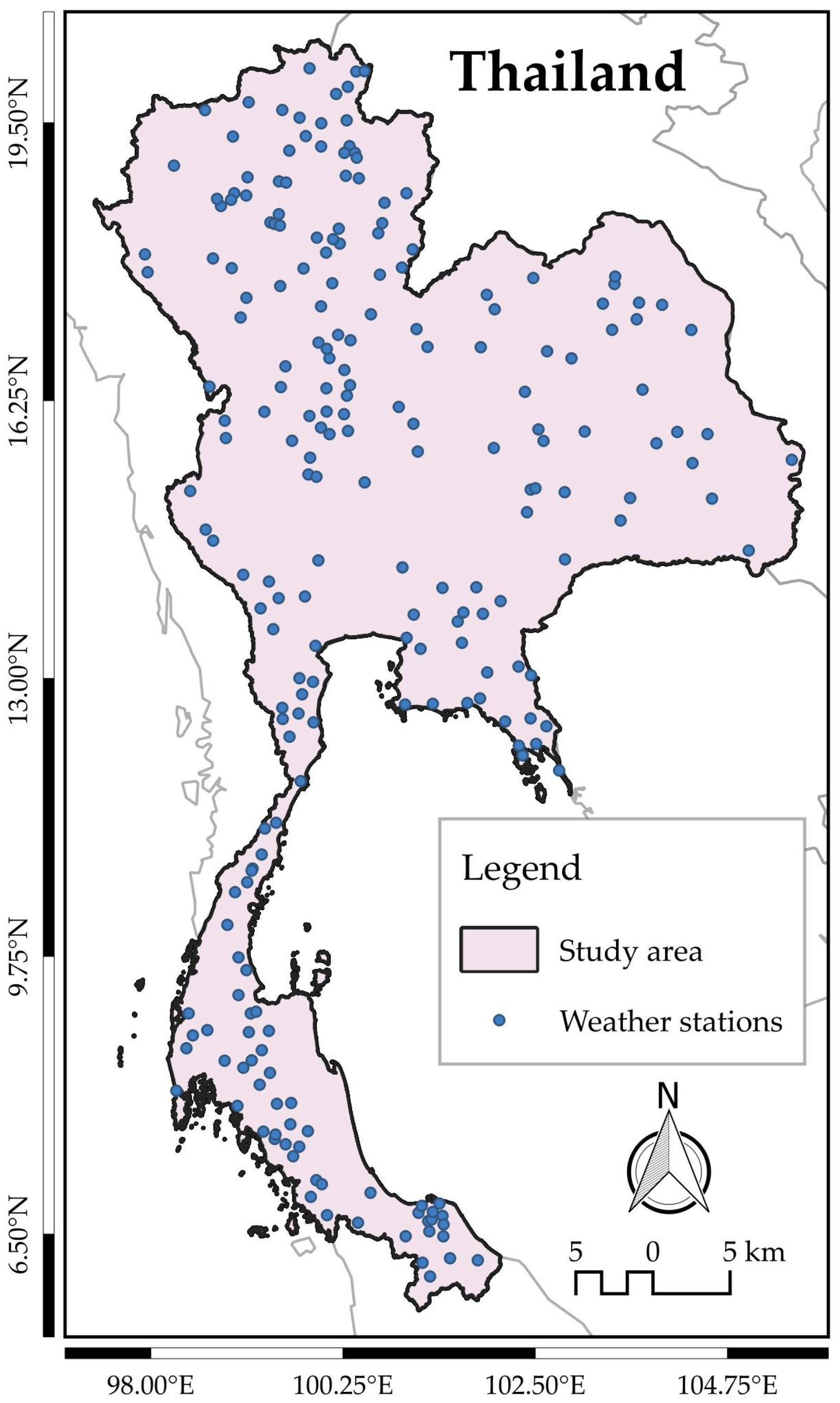
Figure 1. Spatial distributions of weather stations in the study area in 2018.
Preprints 95622 g001
Figure 2. Spatial distribution maps of estimated monthly mean temperature for March, July, and November 2018. Left panels: AST-RK. Right panels: AST-DK.
Preprints 95622 g002
Figure 3. Spatial distribution maps of estimated monthly mean air pressure for March, July, and November 2018. Left panels: AST-RK. Right panels: AST-DK.
Preprints 95622 g003
Table 1. Pearson correlation coefficients between candidate auxiliary variables and target variables, calculated using the entire dataset.
Variable Temperature Air Pressure
Temperature 1.0000 0.5775
Air Pressure 0.5775 1.0000
Relative Humidity -0.2264 0.2204
DEM -0.4284 -0.7577
Table 2. Comparison of temperature and air pressure estimation errors for the FST-RK and FST-DK methods.
Target Variable Auxiliary Variable Error FST-RK FST-DK
Temperature Air Pressure RMSE MAPE 0.8717 2.4435 0.8948 2.4940
Air Pressure Temperature , DEM RMSE MAPE 13.6485 0.7581 11.5184 0.7242
Table 4. Performance comparison of AST-RK and AST-DK for temperature and air pressure estimation.
Target Variable Auxiliary Variable Error AST-RK AST-DK
Temperature Air Pressure RMSE MAPE 0.8660 2.4302 0.8542 2.4099
Temperature Air Pressure , DEM RMSE MAPE 0.8955 2.4803 0.8336 2.3488
Air Pressure Temperature , DEM RMSE MAPE 11.9122 0.7121 10.5835 0.6799
Disclaimer/Publisher’s Note: The statements, opinions and data contained in all publications are solely those of the individual author(s) and contributor(s) and not of MDPI and/or the editor(s). MDPI and/or the editor(s) disclaim responsibility for any injury to people or property resulting from any ideas, methods, instructions or products referred to in the content.
Copyright: This open access article is published under a Creative Commons CC BY 4.0 license, which permit the free download, distribution, and reuse, provided that the author and preprint are cited in any reuse.
Prerpints.org logo

Preprints.org is a free preprint server supported by MDPI in Basel, Switzerland.

Subscribe

© 2024 MDPI (Basel, Switzerland) unless otherwise stated