Introduction
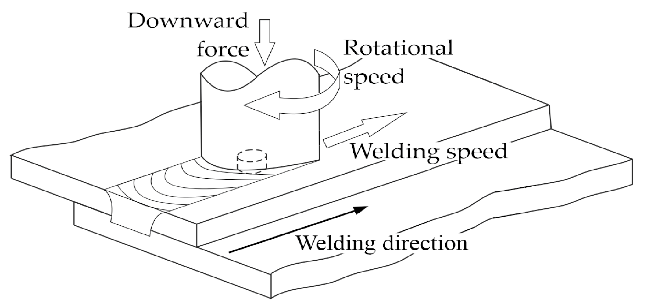
Friction Stir Welding (FSW) is a solid-state welding process that is used to join materials, typically aluminum and other non-ferrous metals, without melting them. It was developed in the early 1990s and owes its popularity to the ability to create high-quality, defect-free welds in challenging materials. The idea of the FSW is given in
Figure 1.
The first patent from 1991 was primarily concerned with controlling the position and speed of the tool during the FSW process. Over the years, FSW technology has evolved considerably. Researchers and engineers have conducted extensive studies and experiments to refine the process and realize its full potential. The beginnings of FSW primarily involved basic control over the tool movement. As research progressed, efforts were made to optimize and improve process parameters. This included a more advanced under-standing of tool rotation speed, plunge depth, traverse speed, and axial force. The goal was to achieve greater control over the flow of the plasticized material, which would result in superior weld quality and mechanical properties.
1.1. Methods of controlling FSW process
In recent years, many different methods have been proposed to control the FSW process to ensure good weld properties. One of the last methods is tool temperature control, which is used to control the rotation speed of the tool. Reports in the literature [
1] indicate that temperature control in FSW allows obtaining better weld properties. However, the process parameters are decisive for each control method. As indicated in [
2,
3] careful selection of FSW parameters allows to avoid the formation of voids or zigzag line defect maximize mechanical properties and regulate fracture location in friction stir weld joints. In the publication [
4] to obtain optimal parameters a response surface (second order) regression model was used for the response, ultimate tensile strength (UTS) of the joints as a function of tool spindle speed, tool transverse speed, downward force and tool tilt angle was developed. To ensure the reliability and accuracy of the developed model, a series of statistical tests were conducted. These tests included Analysis of Variance (ANOVA), the F-ratio, and the assessment of actual and adjusted R-squared (R2) values. These statistical analyses served to evaluate the suitability and effectiveness of the regression model in representing the true relationship between the input parameters and the UTS of the joints. In the work [
5] one-way ANOVA analysis was also performed to analyze the factors influencing weld defects. The application of Taguchi methodology in combination with ANOVA enables the assessment of the statistical importance of various process parameters in relation to the resulting outcomes. In the research described in reference [
6], a comprehensive statistical optimization was carried out using a series of experiments. This optimization process focused on evaluating the ultimate tensile strength (UTS) and elongation of dissimilar joints (AA5454 and AA7075) produced by the friction stir welding.
1.2. Parameters optimization using a machine learning approach
Artificial Intelligence (AI) offers possibilities for predicting and optimizing FSW process parameters. Particularly machine learning techniques, can be employed to develop predictive models [
7,
8,
9,
10,
11]. These models can analyze historical data related to FSW, considering factors such as tool speed, force and material properties, to predict optimal process parameters for the desired outcomes like weld strength, quality, and defect minimization. Study [
8] discusses the development of an integrated prediction model for ultimate tensile strength (UTS), maximum hardness (MH), and heat input (HI) in friction stir welding of AA-7075. The aim of the work was to improve FSW welding procedures by incorporating four control parameters: tilt angle, rotation speed, welding speed, and shoulder diameter. An increasing number of publications present the combination of design of experiments (DOE) and machine learning (ML) as a methodology to collect and analyze data on a specific industrial phenomenon. In this context article [
12] discusses the choice of design in relation to the ML model performances. It's important to note that the effectiveness of AI in predicting and optimizing FSW process parameters depends on the quality and quantity of available data, the choice of AI algorithms, and the specific goals of the optimization. Whether leveraging machine learning techniques, deep learning architectures, or hybrid approaches, the suitability of the chosen algorithms profoundly influences the AI system's ability to discern patterns, generalize insights, and adapt to the complexity of the FSW process. Furthermore, continuous updates to the AI model based on new data and ongoing feedback from the FSW process can enhance its predictive capabilities over time. The successful integration of AI into FSW optimization strategies necessitates a collaborative effort between domain experts, data scientists, and engineers to ensure that the AI system aligns with the evolving dynamics of the welding process.
2. Materials and Methods
The ability of FSW to produce high-strength and high-quality welds without the need for melting the base materials has made it a valuable technology for joining high-strength aluminum alloys like EN AW 7075 . Due to its wide range of applications, this aluminium alloy is still the subject of many studies [
13,
14,
15]. EN AW 7075 is a high-strength aluminum alloy [
16] known for its excellent mechanical properties, which makes it attractive for various aerospace and automotive applications [
15,
17,
18,
19]. FSW offers a promising way to join EN AW 7075 and other similar high-strength aluminum alloys.
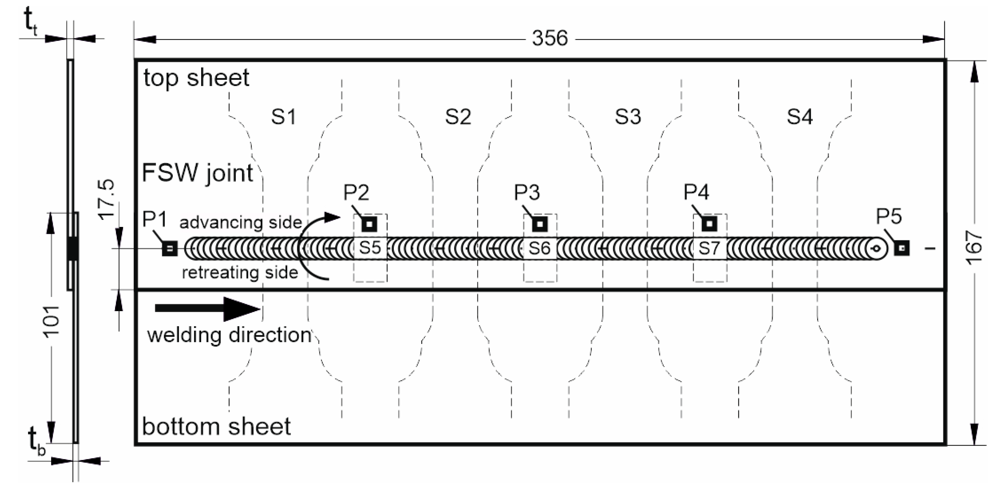
During the experiment, FSW lap joints with a length of 325 mm were produced from the sheet metal pieces measuring 356 mm x 101 mm. Sheet metal of 1.6 mm, 1.0 mm and 0.8 mm thickness was used for the tests. A diagram of the control joint along with the configuration of the thickness of sheet metal to be joined is presented in
Figure 2.
The welding process was carried out on the upper side of the sheet, the thickness of which is given in
Table 1.
EN AW 7075 alloy sheet metal plated on both sides was used in the study. The chemical composition of EN AW 7075 alloy is presented in
Table 2.
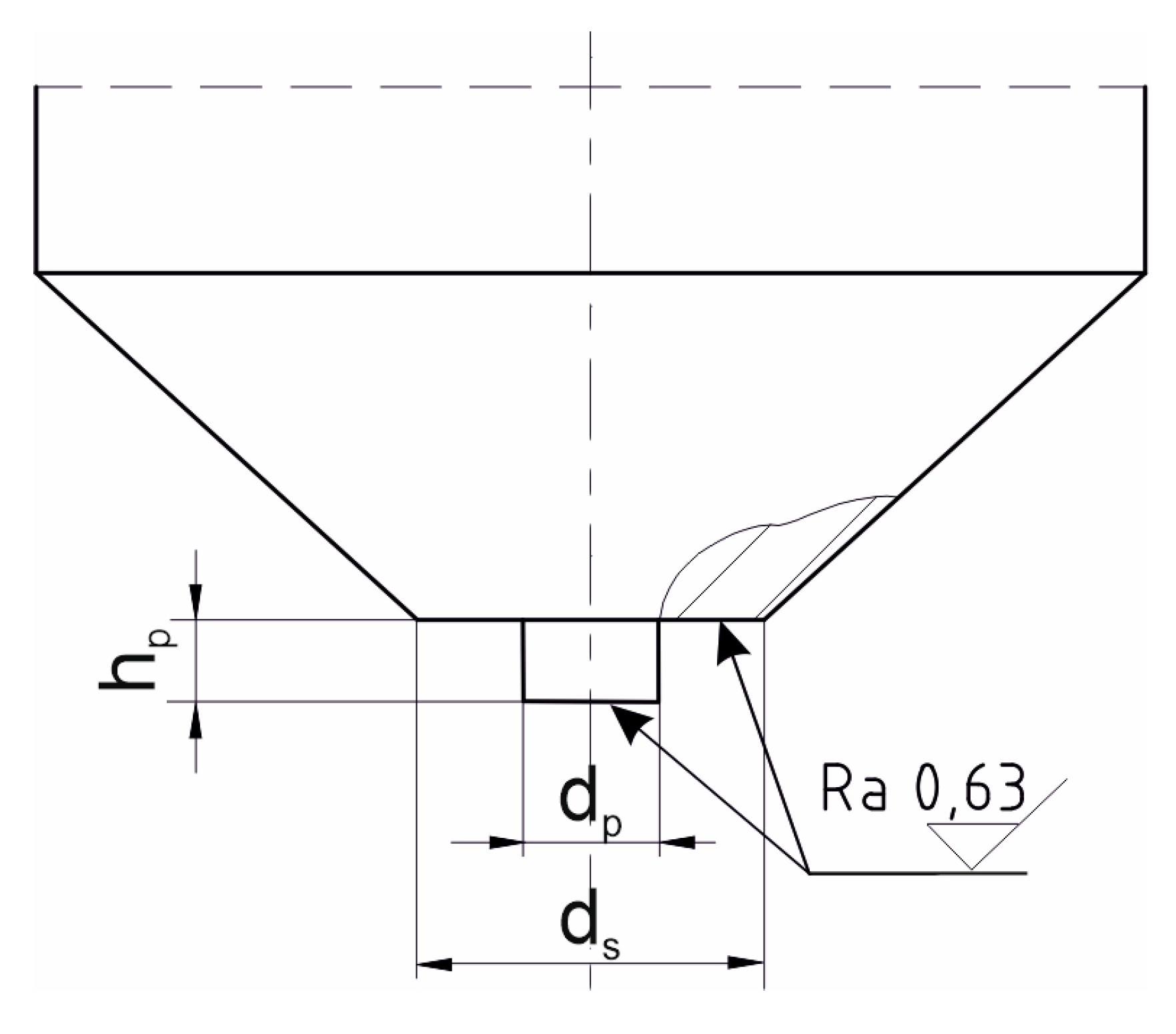
Tools designed by the authors, with a flat shoulder and a cylindrical-shaped pin with a smooth surface, were used to produce the joints. Different shoulder diameters and different pin sizes were tested. The geometry of the working part and the set of tools used for testing are shown in
Figure 3.
Dimension of the working part of FSW tools are shown in
Table 3. T1÷T6 tools were used for producing J1 joints. T2 and T7÷T10 tools were used for J2 joints while J3 joints were made using T11÷T14 tools.
Experimental studies were conducted with different parameters of the welding process: i.e., with variable rotational tool speed n of 700÷6000 rpm and variable welding speed v of 50÷2100 mm/min.
The joints were produced using a CNC machining center with the following parameters: number of controlled axes: 4; X, Y and Z-axis travel: 1040/600/500 mm; table surface area: 1250×600 mm; max. table load: 600 kg; spindle speed: 12,000 rpm; feed rate: 0-40,000 mm/min; spindle motor power: 19 kW.
Four specimens S1÷S4 for strength tests and three specimens S5÷S7 for metallographic tests were cut out from the prepared joints, as marked in
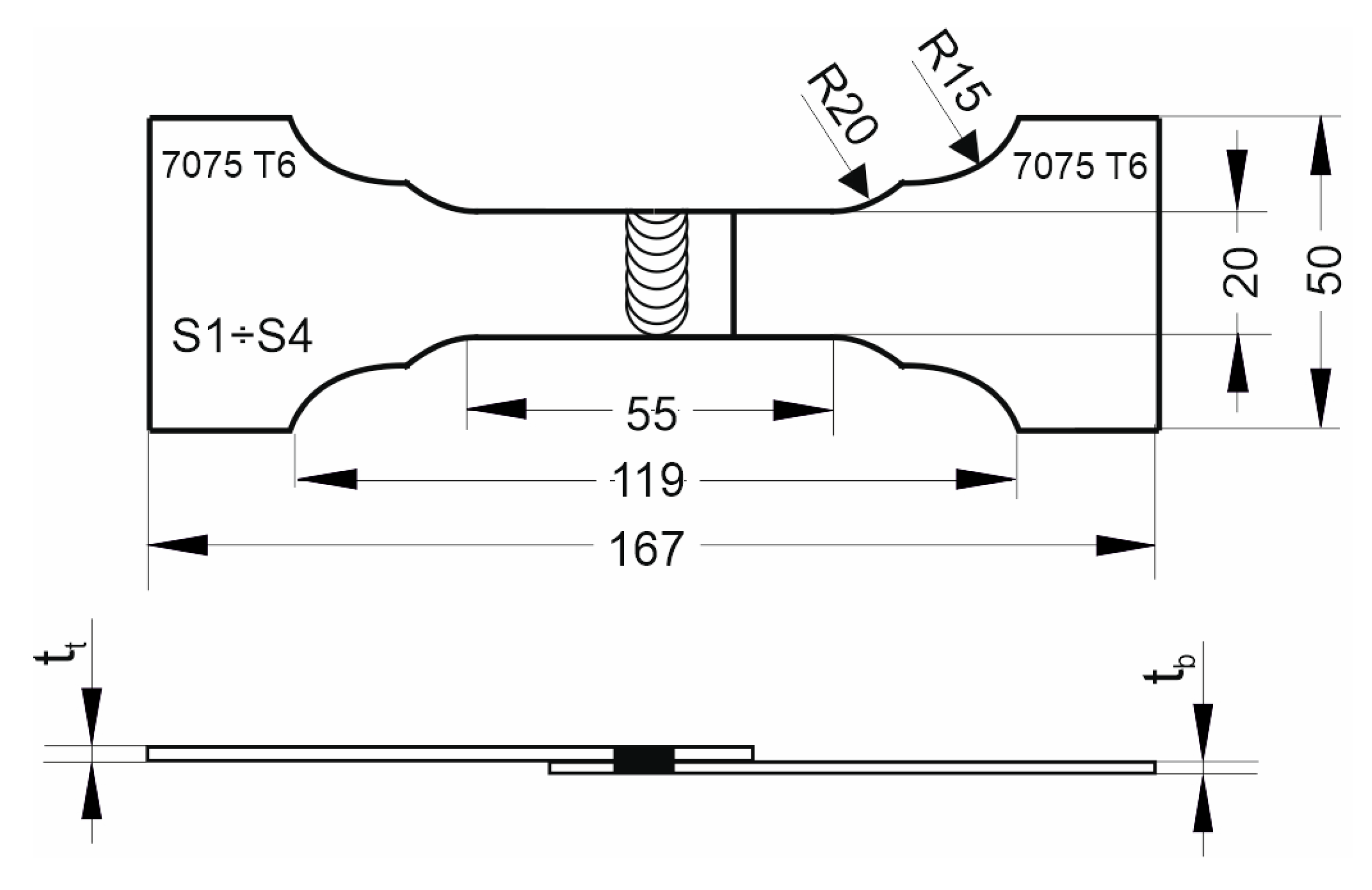
Figure 2. Samples were cut out by abrasive water jet cutting. The geometry of the specimens for strength tests is shown in
Figure 4. The specimens were subjected to a controlled tension until failure using a Zwick Z050 testing machine with a tensile speed of 2 mm/min. The quality of FSW joints was assessed by evaluating the load-bearing capacity and the microstructure on the joint cross-section. The load-bearing capacity was determined as the average value of the force transferred by S1÷S4 samples.
Joints with a load-bearing capacity of not less than 70% of the load-bearing capacity of the base material for the weaker (thinner) sheet metal and joints free of defects such as hooking, cold lap, kissing bond, heterogeneous stirring, and thinning were considered to be of good quality.
3. Development of process parameters using machine learning
Machine learning using neural networks was implemented to develop the parameters of the FSW process. Data from the experiment were used to build the networks. Two types of networks were built: the first one was used to classify good/bad joint, the second one was used to regress the tension load capacity.
A total of 608 samples were used to build for neural network classification and regression, including 98 pieces of joints made of 1.6 and 0.8 mm thick sheets, 228 pieces of joints made of two 1.0 mm thick sheets and 282 of joints made of 1.0 and 0.8 mm thick sheets. In each joint type, the samples were divided into three groups: 70% of the samples were used for teaching the network (learning set), 15% of the samples were used to test the learned networks in order to select the network (testing set) and 15% of the samples were used for validation of the joint quality (validation set). The summary is presented in
Table 4.
3.1. Classification
The random oversampling method was performed in learning and testing sets in each type of joint in such a way as to obtain a similar number of samples in positive and negative classes. Good quality joints were considered as positive class. Then, the sets and types of joints were combined to obtain one database used to build the neural network.
A neural network with a 7-19-2 topology, which consists of one input layer with 7 neurons, one hidden layer with 19 neurons and one output layer with 2 neurons was built. Neurons in the input layer corresponded to the following data from the experiment: thickness of the first sheet, thickness of the second sheet, welding speed, rotational speed, shoulder diameter, pin diameter, pin length. Neurons in the output layer corresponded to the positive and negative classes. Classification was performed using Multi-Layer Perceptron (MLP). Adjusting the weights and bias in the input and hidden layers were used as key factors to bring the results closer to the target and reduce the error rate. A logistic activation function in the hidden layer and a linear activation function in the output layer were used.
Teaching was carried out using the Broyden–Fletcher–Goldfarb–Shanno (BFGS) optimization algorithm. It was assumed that the maximum training time would not exceed 300 epochs. This period was shortened when symptoms of network overlearning were detected. The network learning process was analyzed by observing the change in the value of errors in different learning epochs. The process was stopped before overfitting occurred, as a result of which the error calculated for the test set, instead of stopping decreasing as the error of the training set decreased, began to increase. Sum Square Error (SSE) was applied:
di – dependent variable,
yi – predicted output.
In this study performance of classifier were mainly evaluated with the following evaluation parameters: area under the curve (AUC) receiver operating characteristics (ROC) curve, sensitivity, specificity, precision, negative predictive value and accuracy. Mathematical representation of the evaluation index is as shown in the following Equations:
where:
TP − true positive, a test result that correctly indicates the presence of a condition or characteristic,
TN − true negative, a test result that correctly indicates the absence of a condition or characteristic,
FP − false positive, a test result which wrongly indicates that a particular condition or attribute is present,
FN − false negative, a test result which wrongly indicates that a particular condition or attribute is absent.
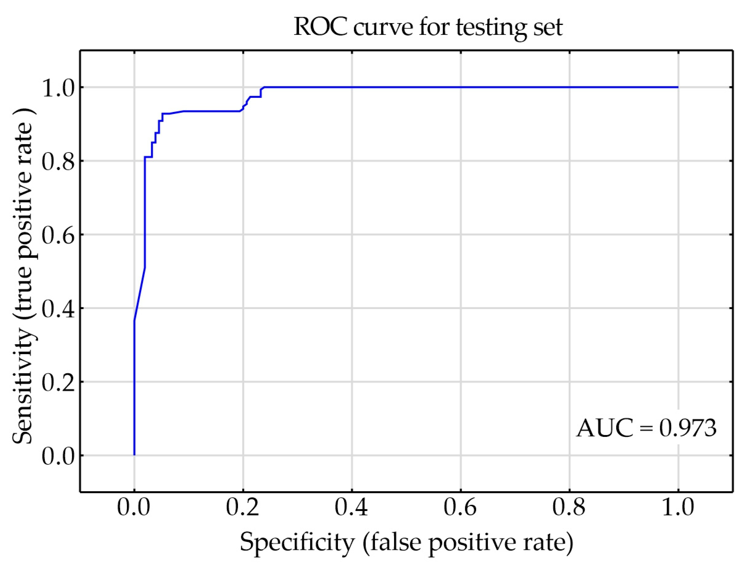
Only 72 epochs were needed to train the network. The receiver operating characteristics (ROC) curve for testing set was shown in
Figure 5. AUC of the designed network was of 0.973. The quality of the testing set was approximately 93.5%. A summary of the neural network is shown in
Table 5.
The degree of efficiency of the neural network is best assessed by showing confusion matrix.
Table 6 shows how many times the diagnoses provided by the network (“prediction class”) for the object specified as belonging to class 1 corresponded to the enough good quality FSW joint (actual class = 1), and how many times the diagnosis prediction class = 0 corresponded with actual class = 0. The cases when prediction class = 0 corresponded with actual class = 1 and vice versa prediction class = 1 corresponded with actual class = 0 represented errors in identification enough good quality FSW joint. As shown in confusion matrix for testing set, the errors never exceeded 6%. This result was assessed as very satisfactory.
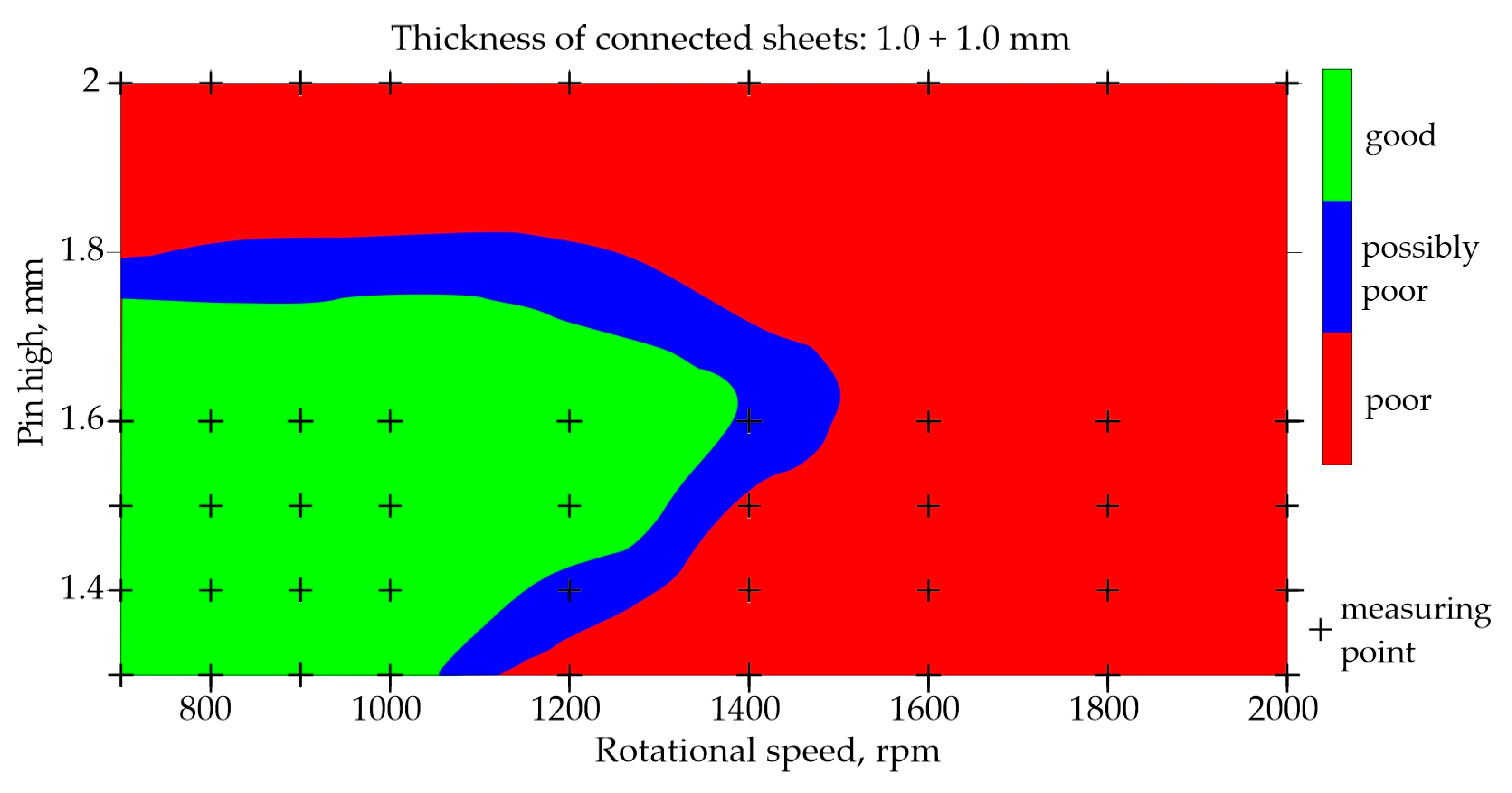
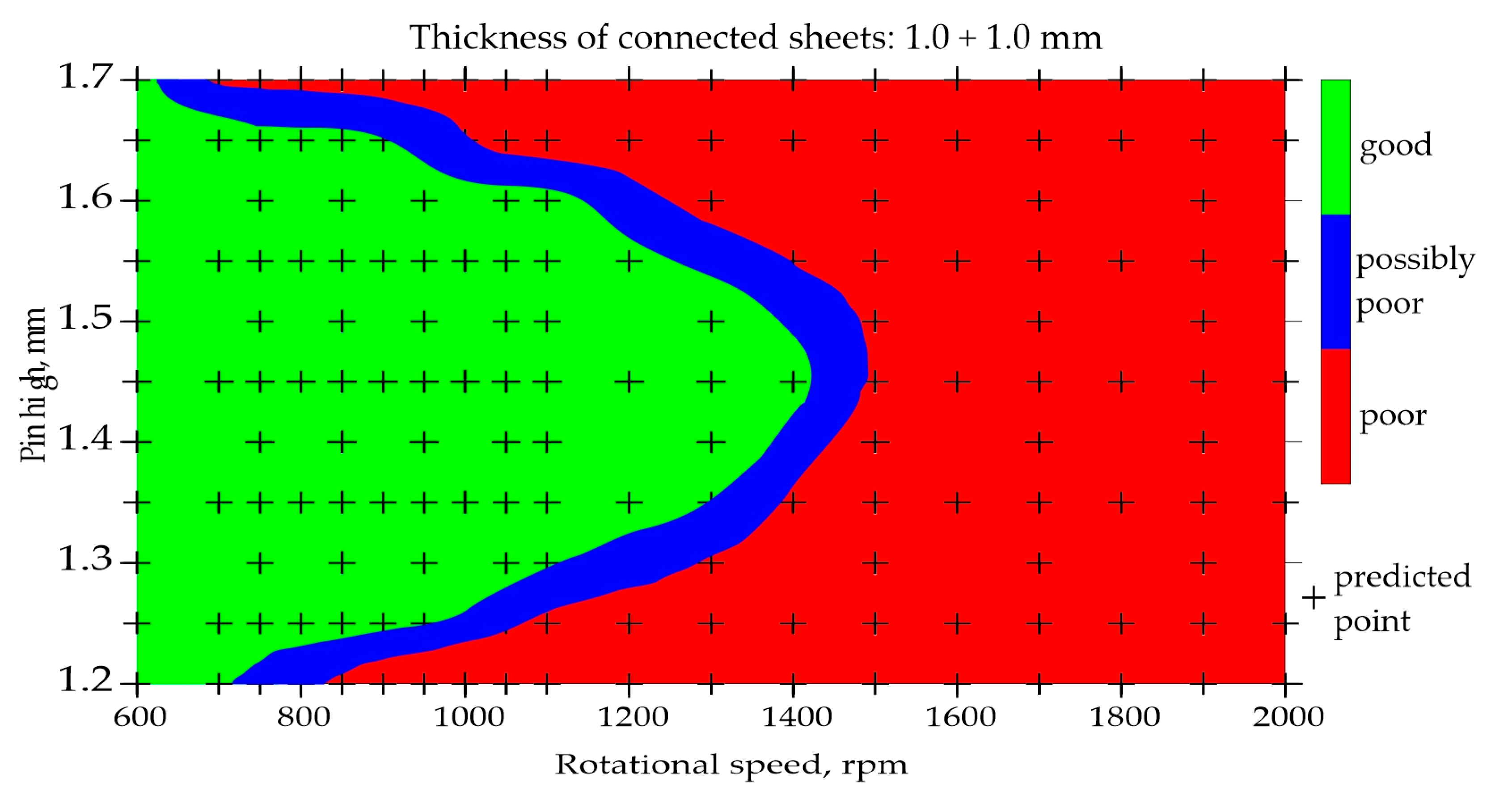
In order to illustrate the prediction capabilities of the classification network, for representative types of joints and representative parameters of the FSW process, the maps shown in
Figure 6,
Figure 7,
Figure 8 and
Figure 9 were built. An orthogonal grid generation model was developed by solving the governing equations of coordinate transformation with a local polynomial collocation method.
The classification of joints made of two 1.0 mm thick sheets is shown in
Figure 6 and
Figure 7. Both figures show the influence of rotational speed and pin height on the quality of the joints. The remaining parameters were constant: welding speed of 150 mm/min, shoulder diameter of 7 mm and pin diameter of 2 mm.
Figure 6 shows the map built on the basis of data from the experiment, while
Figure 7 shows the map built using the developed neural network. The parameters for which poor-quality joints were obtained during welding are marked in red. Parameters that resulted in good quality joints are marked in green. Blue indicates a possible poor joint quality. The places where black crosses appear indicate the welding parameters on the basis of which the maps were developed. The map in
Figure 7 was built solely on the basis of predictions. At the same time, the data range was in-creased, which means that the rotational speed from 600 rpm and the pin length from 1.2 mm were analyzed.
Analyzing the maps in
Figure 6 and
Figure 7, it can be observed that using the tool with the pin length of 1.25 − 1.65, it is possible to obtain good quality connectors at a relatively low rotational speed of up to approximately 900 rpm. When using a higher rotational speed, the tool with a longer pin of 1.35 − 1.6 mm is needed.
The critical rotational speed necessary to obtain good quality joints is approximately 1400 rpm. While the critical length of the pin is 1.7 mm. This is due to the amount of heat generated when joining two sheets of 1.0 mm thick each.
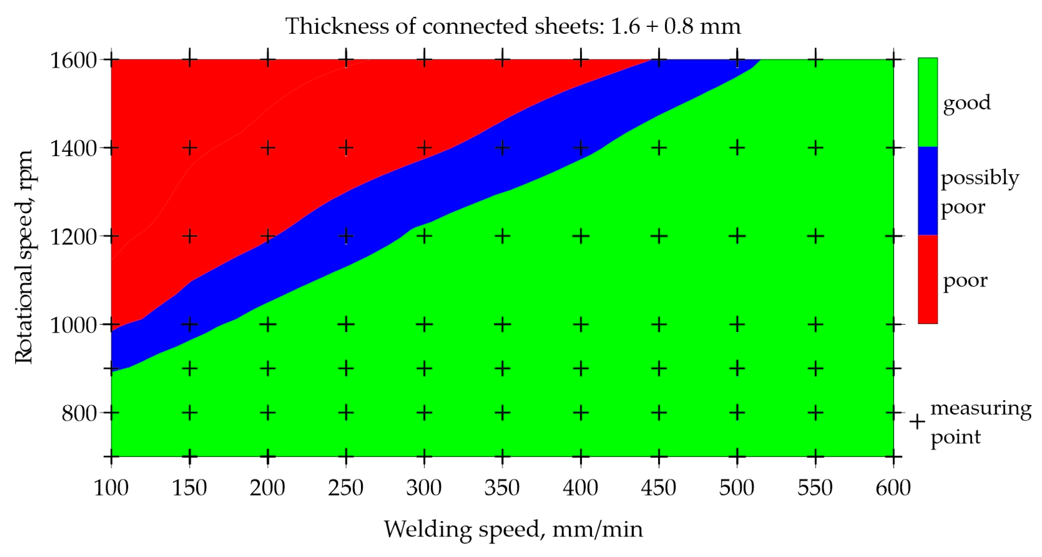
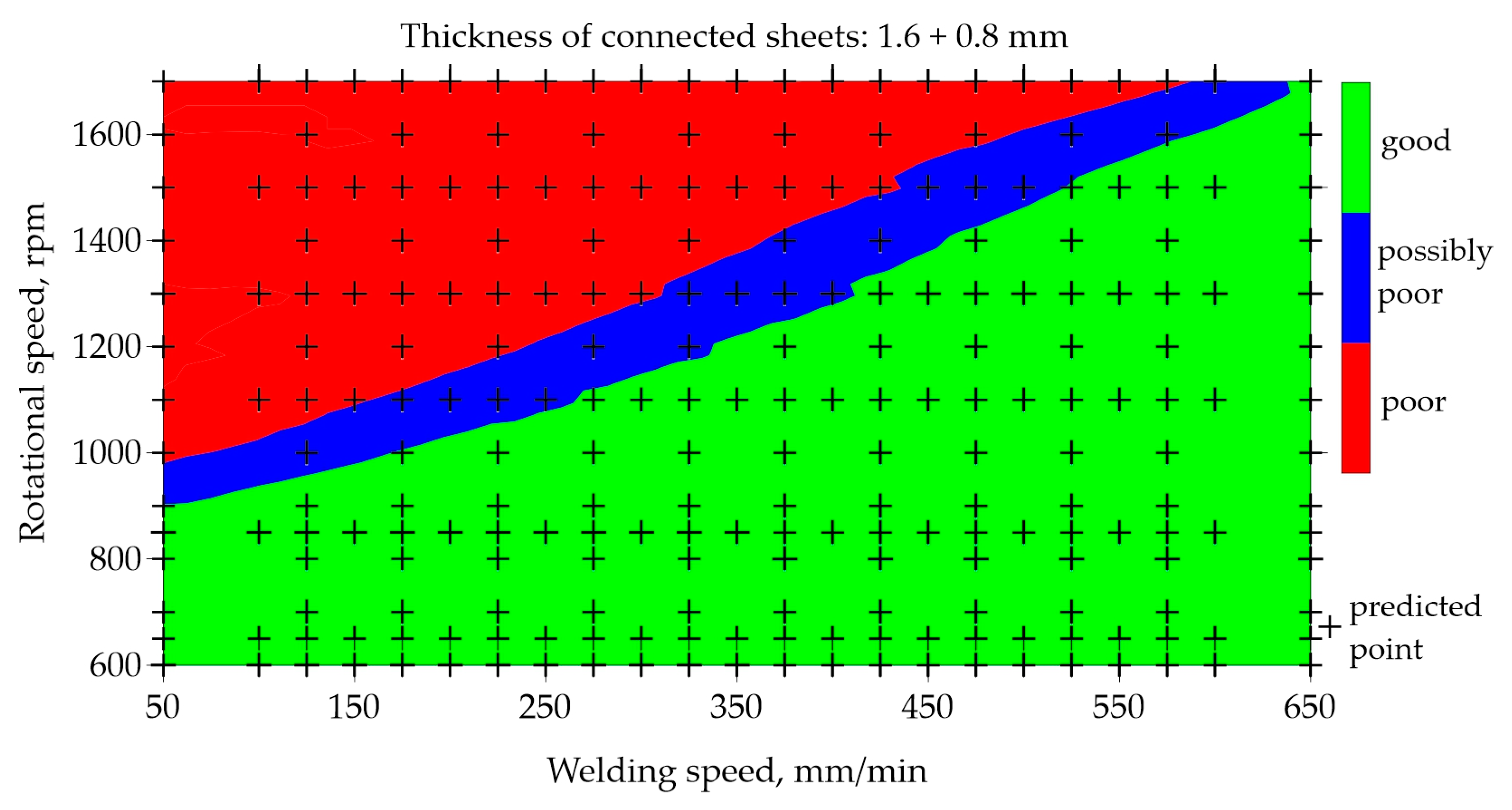
Figure 8 and
Figure 9 illustrate the influence of welding and rotational speed on the quality of FSW joints made of 1.6 and 0.8 mm thick sheets.
Figure 8 shows the map created based on the experimental data used to train the neural network.
Figure 9 shows the map resulting from the prediction of the neural network for classification. As in the previous example, poor quality joints are marked in red, good quality joints are marked in green, and blue indicates the possible poor quality. The results are presented for the samples made using T12 tool. The welding speed in the network learning set was in the range of 100 − 600 mm/min, and the rotational speed was in the range of 700 − 1600 rpm.
The prediction was developed for an extended range of welding speed from 50 to 650 mm/min and the rotational speed in the range of 600 1700 rpm. Prediction was per-formed only for data on which the network was not trained, which is marked with black crosses. Analysing the welding parameters generating good-quality joints made of 1.6 and 0.8 mm thick sheets, it can be seen that it is possible to use any welding speed ranging from 50 to 650 mm/min, while using a low rotational speed up to 900 rpm.
An almost linear relationship was observed, which shows that by increasing the rotational speed above 900 rpm, the welding speed should also be increased. This is caused by the amount of heat generated by the tool. To obtain the good-quality FSW joint, a certain constant amount of heat must be supplied to the welded sheets. The amount of heat depends on the thickness of the joined sheets and the type of tool used. A specific amount of heat can be obtained as a result of the small welding speed and the relatively low rotational speed. The same amount of heat can be obtained by increasing the welding speed and simultaneously in-creasing the rotational speed.
3.2. Regresion
To predict the load-bearing capacity of the joint, another neural network was built for regression. To develop the network, the same samples like in the classification network were used, i.e. a total of 608 samples. The same sample labelling as in the classification network was used to assign samples to the learning, testing and validation sets
Table 4.
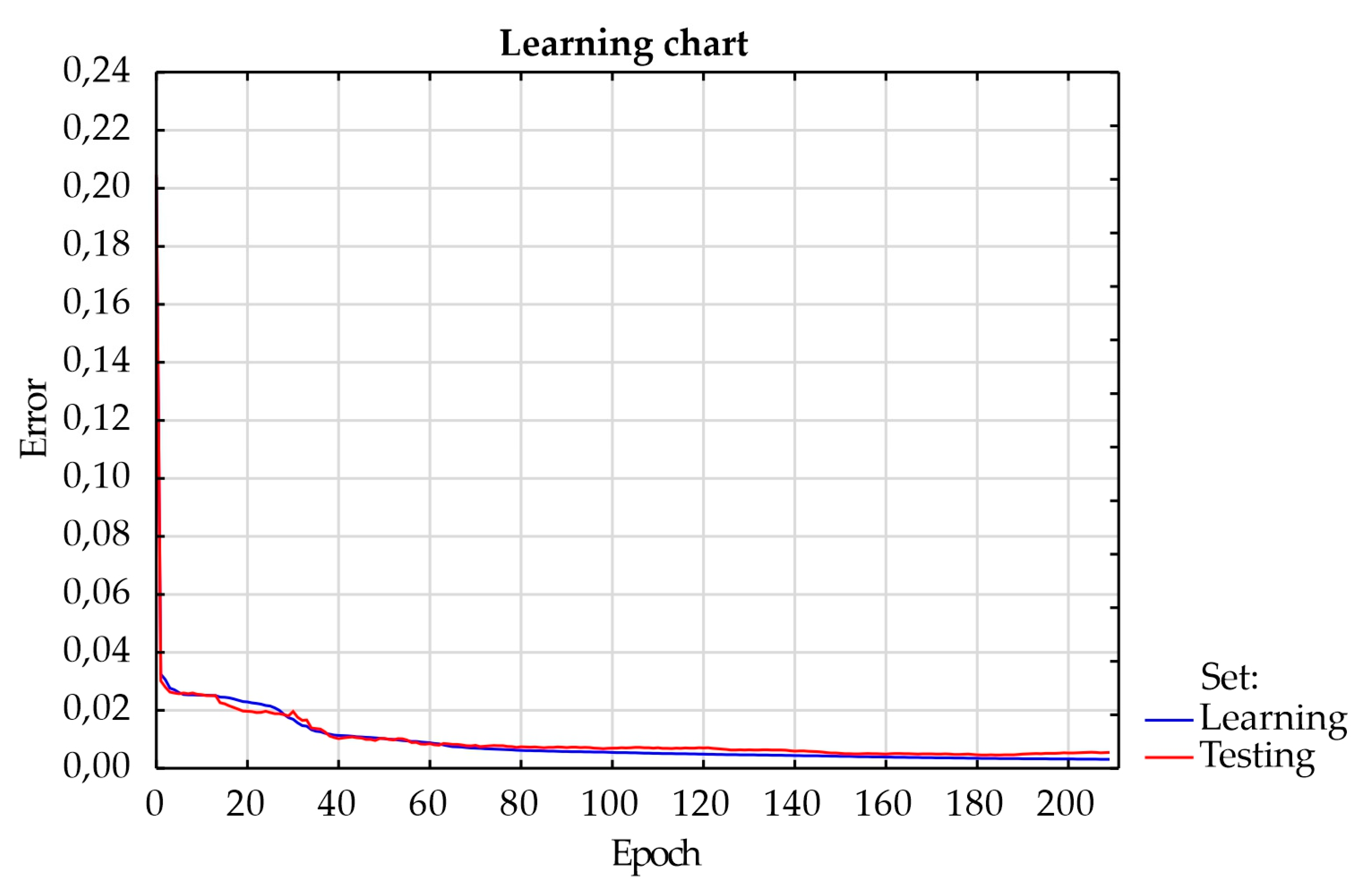
A neural network with a 7-19-1 topology was built. This means using the input layer with 7 neurons, one hidden layer with 19 neurons and the output layer with 1 neuron. Neurons in the input layer corresponded to the following data from the experiment: thickness of the first sheet, thickness of the second sheet, welding speed, rotational speed, diameter of shoulder, diameter and length of pin. Neuron in the output layer corresponded to the load-bearing capacity of the FSW joint. Regression was performed using Multi-Layer Perceptron. Adjusting the weights and bias in the input and hidden layers were used as ingredients to reduce the error rate. A hyperbolic activation function tanh was used in the hidden layer and a linear activation function was used in the output layer. Learning was performed using the BFGS optimization algorithm. It was assumed that the maximum training time would not exceed 200 epochs. As in the case of classification, the regression network learning process was assessed by observing the change in SSE error values. Analysing the graph of the artificial neural network learning process (
Figure 10), it was found that 184 epochs were necessary to train the network. Thanks to this, the network had sufficient approximation and generalization ability. The accuracy of the testing set was approximately 92.5%. A summary of the neural network is shown in
Table 7. However,
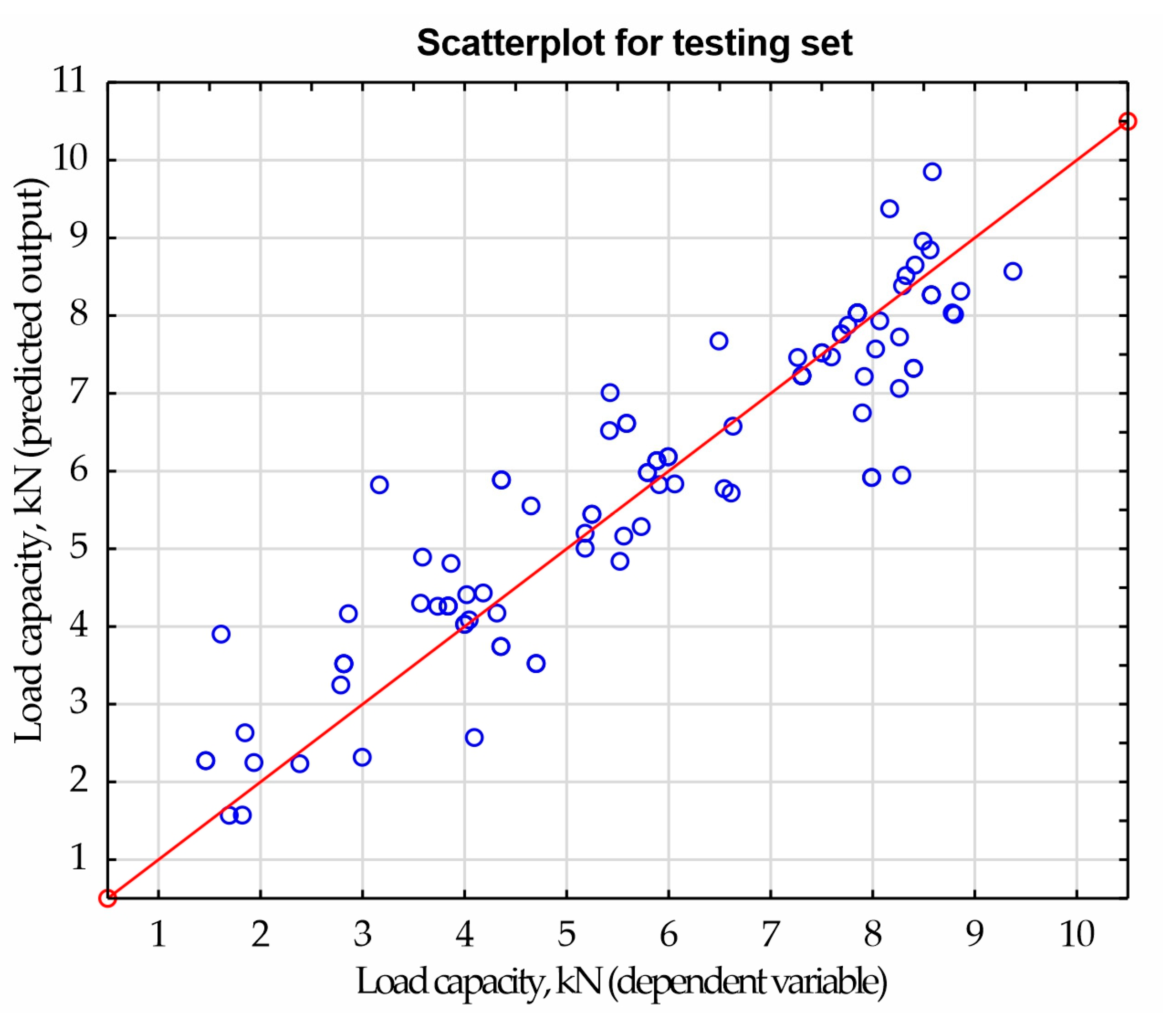
Figure 11 shows a scatterplot between the dependent variable and the predicted response of load-bearing capacity, thanks to which the quality of the model was diagnosed.
The possibility of predicting the neural network for regression was presented on the basis of data for the representative type of joint made of 1.0 and 0.8 mm thick sheets. Maps illustrating the relationship between the welding speed and rotational speed for tools T1 and T4 are shown in
Figure 12,
Figure 13,
Figure 14 and
Figure 15. The grid generation model was developed by the local polynomial method.
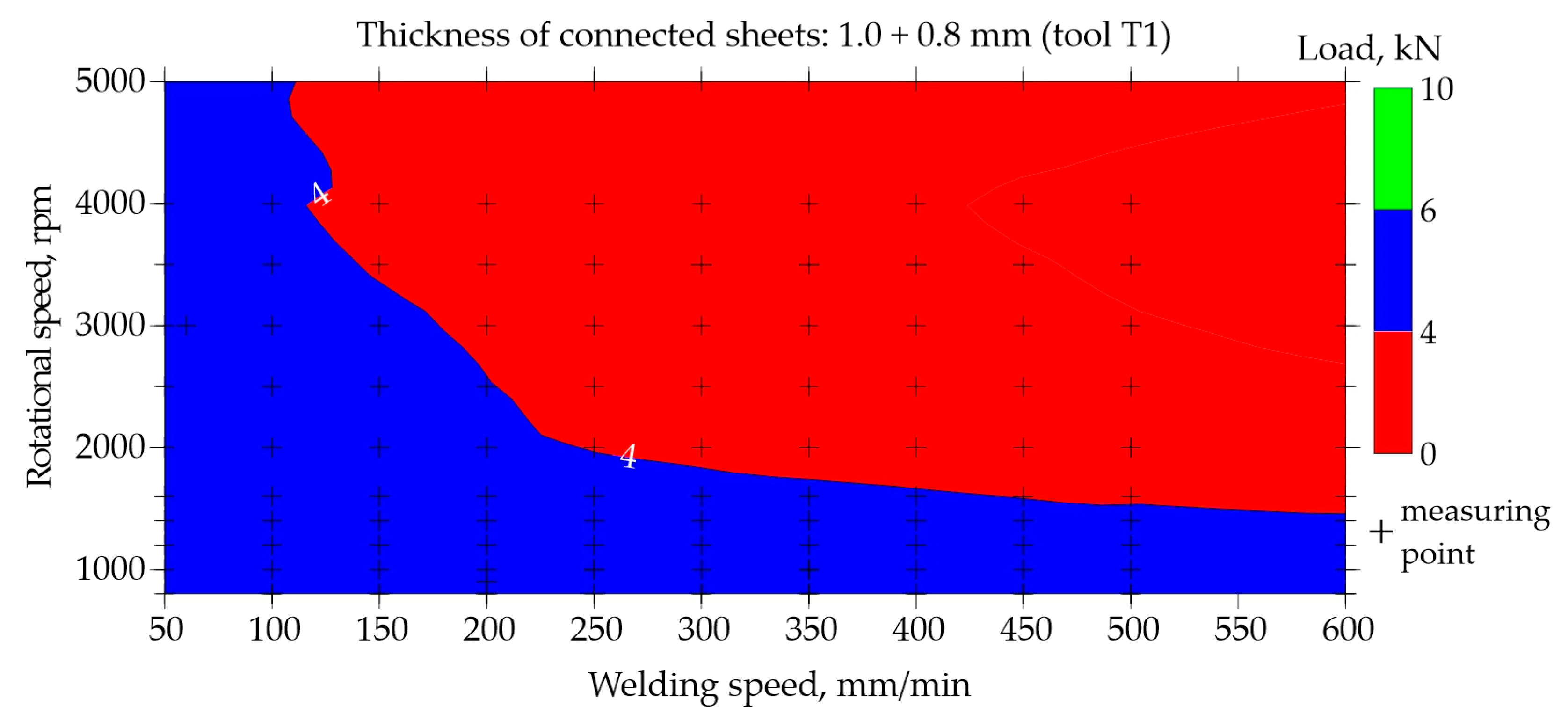
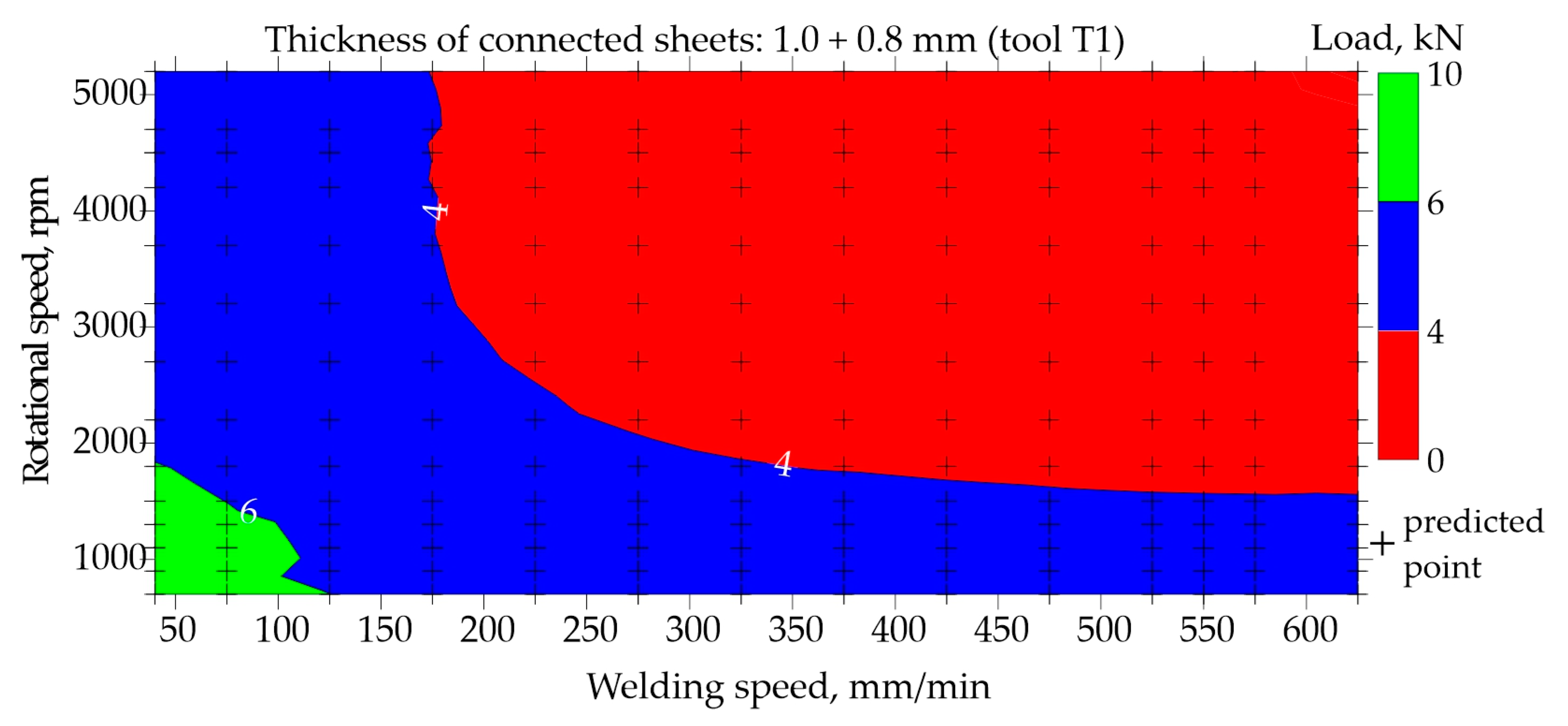
Maps for assessing the load-bearing capacity of joints made using the T1 tool with the shoulder diameter of 7 mm, pin diameter and length of 2 mm and 1.2 mm were shown in
Figure 12 and
Figure 13.
Figure 12 shows the map based on experimental data that was used to train the network. Load capacity equal to or greater than 6.0 kN is marked in green. It can be interpreted as the load capacity desired by the joints, since the minimum acceptable load capacity is 5.8 kN. As can be seen from
Figure 12, no areas marked in green were observed. However, it can be observed that when welding joints using the T1 tool, the highest load-bearing capacity is achieved by joints welded at low rotational speed up to 1600 rpm.
The map resulting from the network prediction is shown in
Figure 13. The results are presented for an enlarged area of welding speed in the range of 40 − 650 mm/min and rotational speed in the range of 700 − 5200 rpm. Using the ability to approximate and generalize the constructed neural network, a small area marked in green was observed in
Figure 13, which means it is possible to weld FSW joints using the T1 tool in such a way that their load capacity exceeds 6.0 kN. For this purpose, a low welding speed of 40 − 50 mm/min and a low rotational speed to approximately 1600 rpm should be used.
Both figures
Figure 12 and
Figure 13 show that FSW welding using the T1 tool with high welding speed and high rotational speed results in joints with a very low load-bearing capacity not exceeding 4.0 kN.
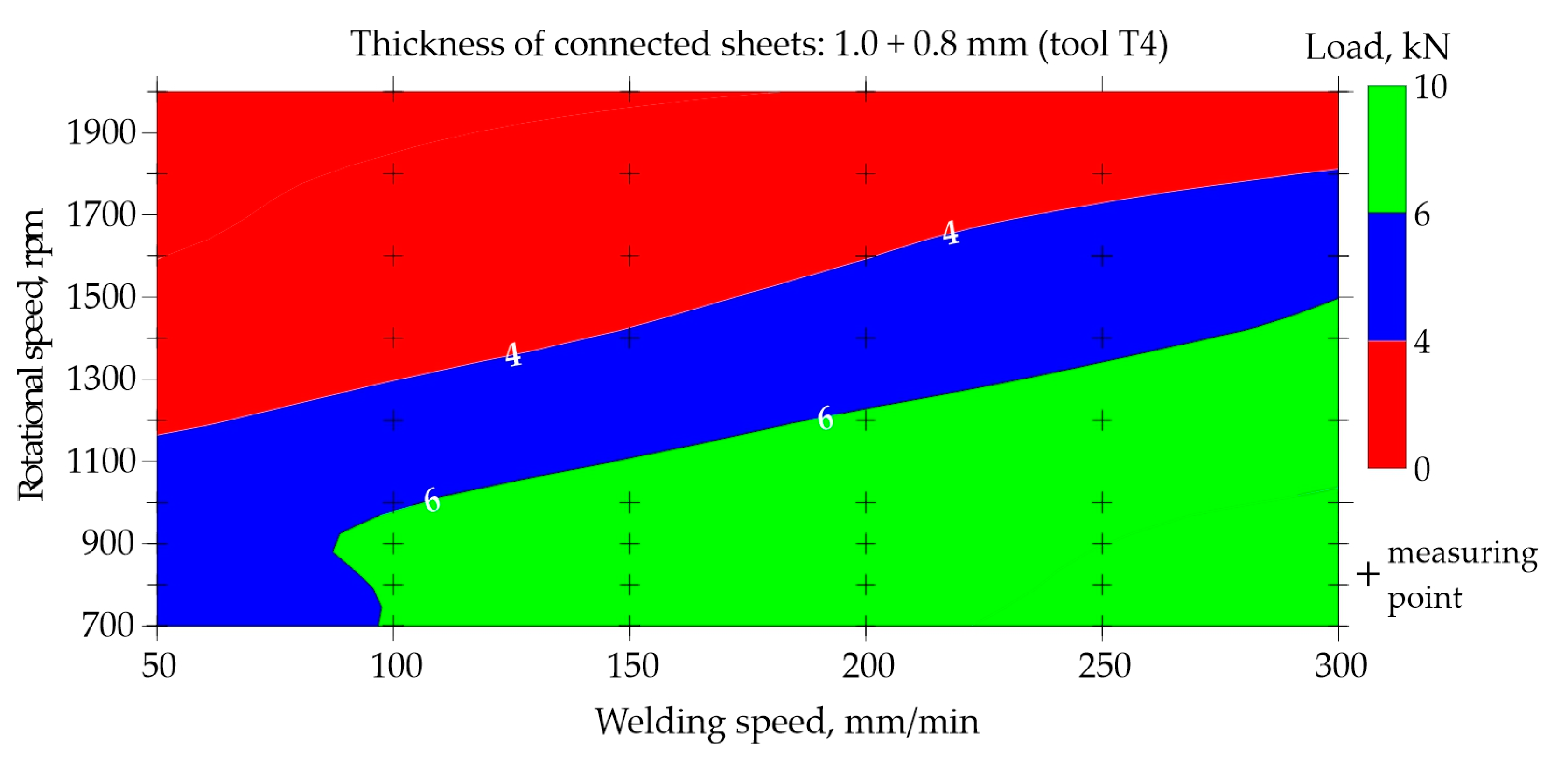
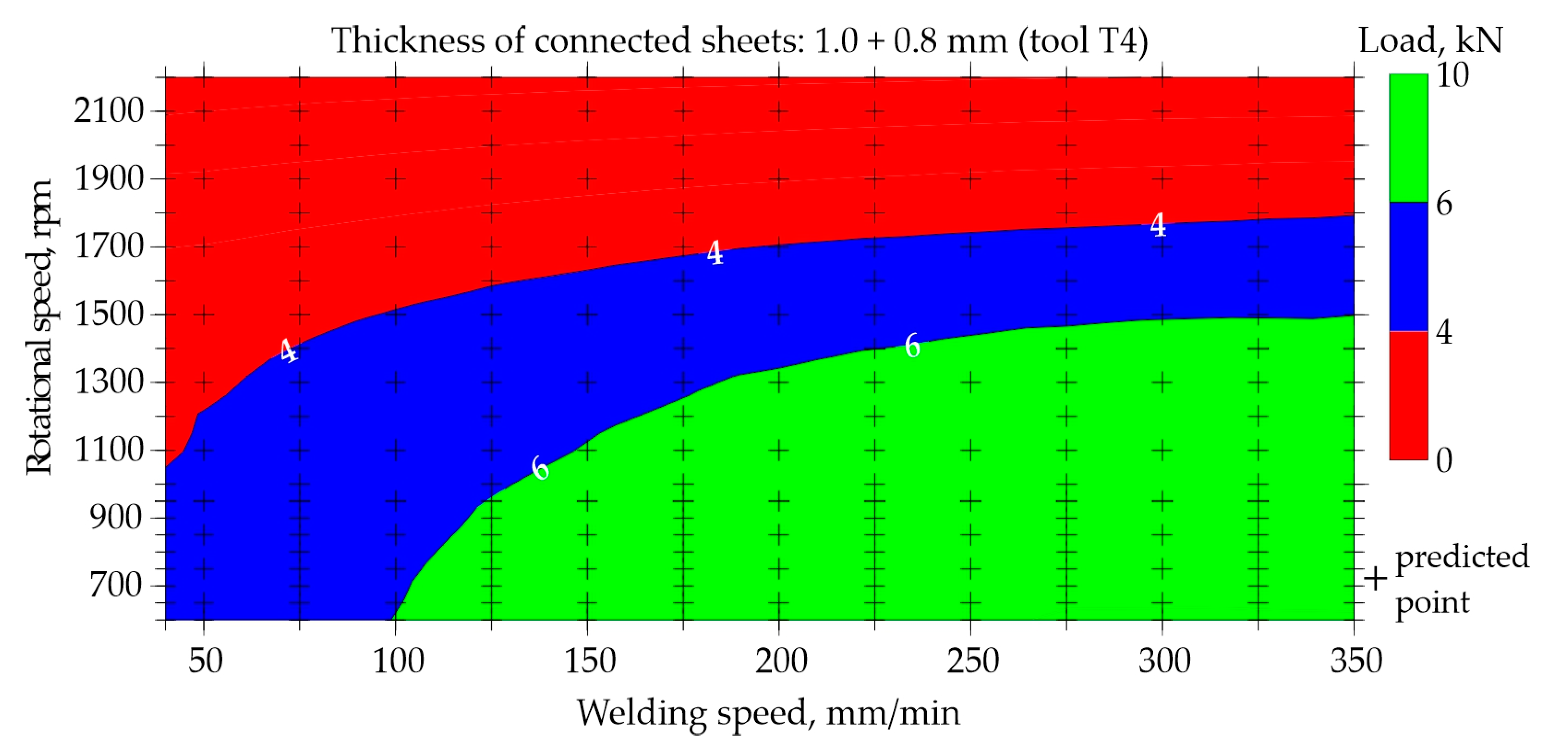
Maps for assessing the load-bearing capacity of joints made using the T4 tool with the shoulder diameter of 10 mm, pin diameter and length of 4 mm and 1.86 mm, respectively, are shown in
Figure 14 and
Figure 15. Experimental data were used to prepare
Figure 14. It is easy to observe a large area of FSW process parameters, which are used to weld joints with a load capacity exceeding 6.0 kN. The best joints transfer a force of approximately 8.5 kN. To make such joints, it is necessary to set a low rotational speed of 700 − 1000 rpm and a fairly high welding speed, at least 200 mm/min. Reducing the welding speed below 150 mm/min and simultaneously increasing the rotational speed above 1300 rpm results in a significant reduction in the load-bearing capacity of the joints to below 4.0 kN, which is marked in red.
Very similar relationships were observed in
Figure 15, which was developed on the basis of neural network predictions. Even taking into account the extended range of welding speeds of 40 − 350 mm/min and rotational speeds of 500 − 2200 rpm, it was found that the highest load-bearing capacity of the joints is achieved by using a relatively high welding speed and low rotational speed. The developed maps (
Figure 12,
Figure 13,
Figure 14 and
Figure 15) also allow for the assessment of the impact of the tool itself on the quality of joints. FSW joints made using the T4 tool with a larger shoulder diameter of 10 mm show a much higher load capacity of approximately 8.5 kN than joints made using the T1 tool, in which the shoulder diameter is smaller and amounts of 7 mm. The load capacity of joints welded using the T1 tool is approximately 6.0 kN at most.
When using the T1 tool with the shoulder and pin diameters of 7 and 2 mm, to obtain the joint with an acceptable load-bearing capacity, a low welding speed of 40 − 50 mm/min and a low rotational speed of approximately 700 − 1600 rpm should be used. However, using a larger tool with the shoulder and pin diameters of 10 and 4 mm, the best joints are obtained by conducting the FSW welding process at a higher welding speed of 200 − 300 mm/min and an equally low rotational speed of 700 − 1000 rpm. A tool with greater shoulder causes the welded material to accumulate more heat. Therefore, a higher welding speed is required. It should also be taken into account that the T1 tool had the pin length of 1.2 mm and the T4 tool had the pin length of 1.86 mm. The longer pin results in the larger volume of mixed material, thereby improving the quality of the FSW joint.
4. Case study
This work uses a case study as a research method to examine a specific connector in the broader context of neural network applications and thus draw more general conclusions. The knowledge obtained from the case study will be used to better understand the FSW process and to improve real actions. The basic parameters of the FSW process with which the joint was made were rotational speed n = 700 rpm and welding speed v = 100 mm/min. The choice of the J1 joint as a case study was due to the relatively large problems occurring in manufacture of this type of joints due to the use of thin sheets. The parameters for making the joint were selected based on the assessment of charts
Figure 14 and
Figure 15. Map based on training data in the area of parameters n = 700 rpm and v = 100 mm/min showed a slight discrepancy with the map based on prediction.
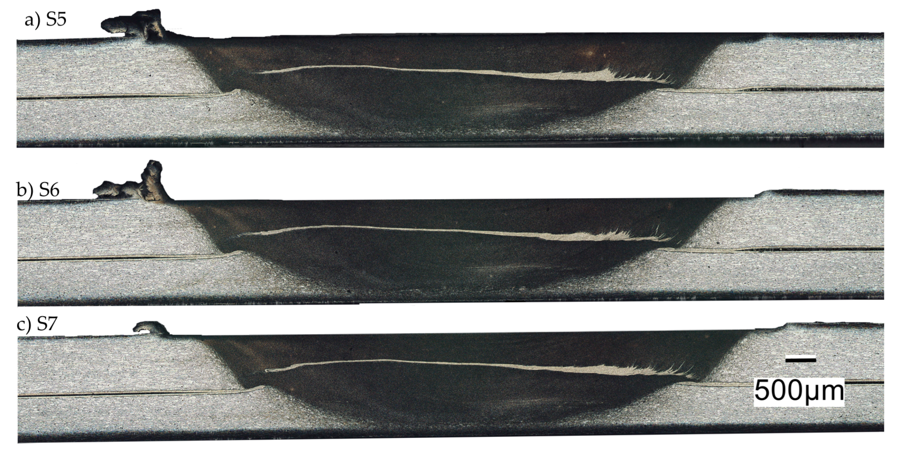
Figure 16 depicts the macrostructure of the J1 joint across three distinct sections. The sampling locations for specimens S5, S6, and S7 are illustrated in
Figure 2. The accompanying images reveal three macrostructures characterized by the absence of observable structural defects. The lighter region corresponds to the base material, while the darker region represents the stir zone. A line of aluminium clad is visible in the centre of the stir zone. In [
21,
22], it was determined that ultrasonic testing enables differentiation among various joint types, specifically: joints devoid of material discontinuities, joints with material discontinuities on the leading side, and joints characterized by discontinuities extending across the entire width of the mixing zone. The investigation specifically considered horizontally oriented defects. However, the application of a similar methodology to assess J1 joints did not identify any material discontinuities in the examined samples.
Modelling of the FSW process allows insight into the complex phenomena occurring in the FSW process. Finite element analysis models can predict the likelihood of defects such as voids, inclusions, or improper material mixing in a welded joint. In the current version of the neural network, the heat input index has not been included, but further work will lead to its inclusion, which will provide the neural network with new forecasting capabilities.
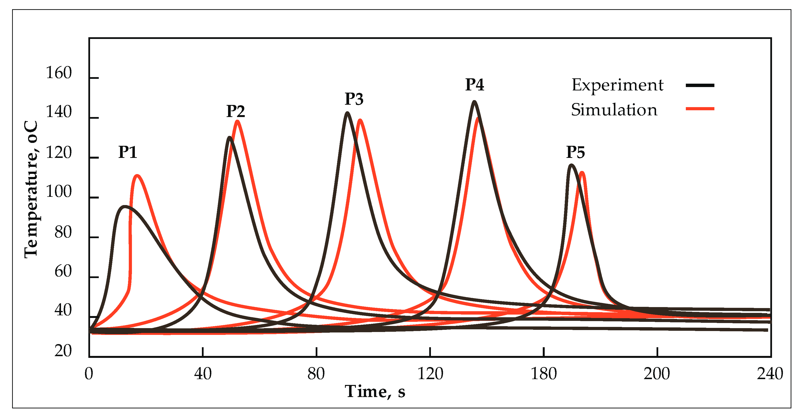
Figure 17 presents a comparative analysis of temperature measurements obtained from experimental data and those calculated using the finite element method. The numerical model employed in this study is explicated in the authors' prior works, notably [
23]. In this work the thermal model considered heat conduction and convection, allocated to pertinent structural elements. Temporal functions were employed to characterize the movement of the heat source. The numerical model incorporated both the welding and clamp release stages. The simulation output encompasses the temperature field, residual stresses, and deformations manifesting within the welded structure. The maximum disparity between the calculated and measured temperature peaks is within 14%, specifically for the thermocouple positioned at point P1. Discrepancies between experimental measurements and numerical simulations arise from challenges associated with accurately determining the thermocouple positions during the experiment and variations in process parameters attributable to frictional resistance encountered in the process.
The predictive capabilities of the developed neural network model indicated, based on map
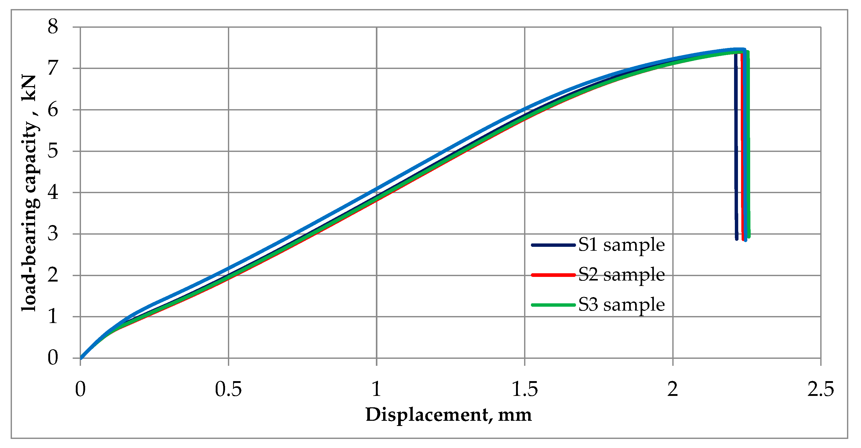
Figure 15, that the load-bearing capacity of the made joint J1 would be in the range of 4-6 kN. However, a static tensile test performed for four samples S1-S4 cut from joint J1 according to the diagram in
Figure 2 showed that the load capacity of the joint is higher and is in the range of 7-8 kN as shown in
Figure 18. The tests carried out showed that for the analysed case the neural networks predicted a lower load-bearing capacity of the joint than the tests showed. Neural networks, despite their effectiveness, are subject to inherent limitations and potential inaccuracies. Common challenges and sources of inaccuracy in neural networks often emanate from the quality and quantity of the available data. The quality of data, including its relevance, accuracy, and representativeness, significantly influences the model's ability to discern pertinent features and generalize effectively. In instances where data inadequacies prevail, models may encounter difficulties in capturing the underlying patterns, leading to compromised performance. Addressing these challenges necessitates a comprehensive understanding of the data intricacies and the implementation of strategies to enhance the robustness and generalization capabilities of neural network models in diverse contexts.
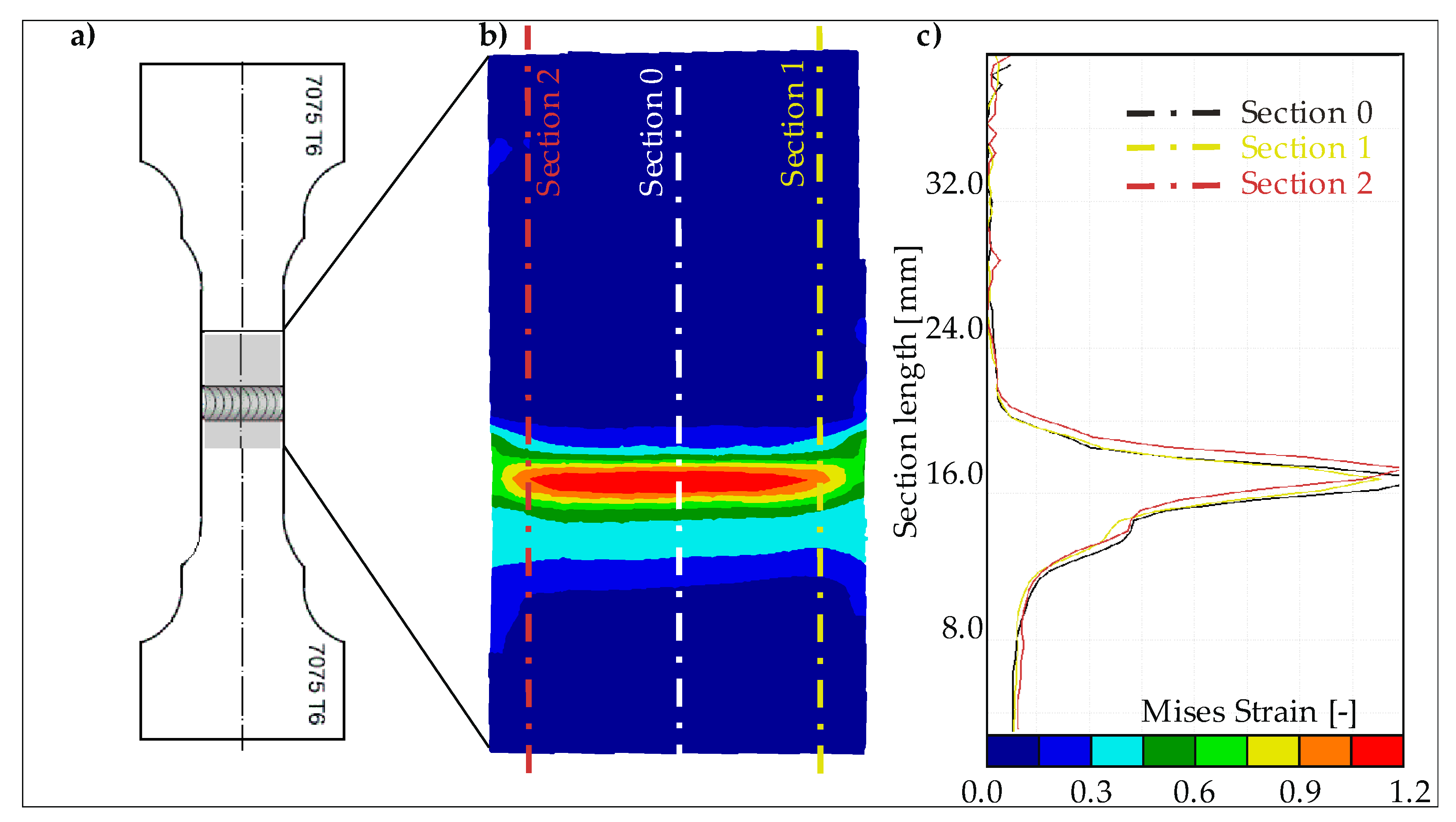
Tensile tests were recorded using a GOM Aramis system for non-contact real-time analysis of specimen deformation. The system consists of two cameras and two lamps that illuminate the measurement area and a computer workstation with special software that allows digital correlation of the recorded images. The Aramis system analyses the displacements of the measuring points from which it calculates the values of Mises strain field occurring in the sample due to the load applied. Within this context, there is intention to employ the Mises strain field of the fracture zone for training neural networks in forthcoming research.
Figure 19 shows the Mises strain field, on a sample before rupture, obtained when stretching sample S4 in a tensile test. The utilization of this strain field as a training dataset for neural networks is anticipated to provide valuable insights into the relationship between material deformation and fracture behaviour.
The application of such a dataset in neural network training holds promise for enhancing the predictive capabilities of models focused on fracture prediction and related mechanical properties. This approach aligns with the broader objective of leveraging advanced computational techniques to deepen our understanding of material behavior under stress conditions, ultimately contributing to advancements in fracture mechanics and structural integrity assessments.
Limitations of the neural network model for predicting FSW process parameters
To obtain correct predictions about the joint load-bearing capacity in the Friction Stir Welding (FSW) process, it's essential to provide the neural network with relevant and comprehensive data related to the welding conditions, material properties, and other pertinent factors. The following types of data are crucial for training a neural network to predict joint load-bearing capacity accurately:
Welding Parameters. Data on key FSW parameters such as rotational speed, welding speed, axial force, joint and tool geometry. These parameters significantly influence the heat generation, material flow, and overall welding process. Based on the authors' previous research, a set of arbitrarily selected parameters, marked in bold, were used as input data for training the network.
Material Properties. Information about the properties of the materials being welded, such as thermal properties, and mechanical properties. Different materials may respond differently to the welding process, affecting joint load-bearing capacity.
Temperature Profiles. Temperature data at various locations within the weld zone during the FSW process. Temperature profiles are critical for understanding the thermal history of the joint, which directly impacts its load-bearing capacity.
Force Measurements. Data on the forces applied during the welding process, including axial force and any additional forces or loads. Force measurements are directly related to the mechanical aspects of joint formation and can influence the joint strength.
Deformation and Strain Data. Information on the deformation and strain experienced by the material during welding. This data is essential for understanding how the material responds to the welding forces and thermal effects.
Microstructure Information. Details about the microstructure of the welded joint, including grain size, grain orientation, and any potential defects. The microstructure has a direct impact on the mechanical properties of the joint.
Previous Joint Performance Data. Data from previously welded joints with known load capacities. This historical data can help the neural network learn patterns and correlations between input parameters and joint load capacity.
Frictional Effects. Data on frictional effects during the FSW process, as these can influence the heat generation and material flow. Frictional forces between the tool and the workpiece are crucial factors in predicting joint load capacity.
Tool Wear Information. Data on tool wear over time. Tool wear can impact the quality of the weld and, consequently, the joint load capacity.
Welding machine and equipment. The type of machine used, especially its stiffness and the FSW joint mounting system in the welding machine, may affect the quality of the weld.
Environmental Conditions. Environmental conditions, such as ambient temperature and humidity, as these factors can influence the overall welding process.
It's important to preprocess and normalize the data appropriately before feeding it into the neural network. Additionally, a sufficient amount of diverse and representative data is crucial for training a robust model capable of making accurate predictions for joint load capacity in FSW. The insights from the analysis presented in the case study will serve as a valuable resource for a deeper understanding of the friction stir welding (FSW) process in the context of neural network training. The knowledge gained is expected to not only increase our understanding, but also play a key role in refining and optimizing practical applications of neural networks and FSW processes.
5. Conclusions
By integrating the knowledge gained from the case study into the training processes of neural networks, there exists a promising avenue to enhance the predictive capabilities and efficacy of these computational models. The nuanced understanding of the FSW process, garnered through the analysis, is expected to provide valuable inputs for developing and fine-tuning neural network architectures specifically fitted for applications related to FSW processes. Based on the experience obtained in this work, the following conclusions can be drawn:
Selected parameters of FSW process: rotational speed, welding speed, joint and tool geometry used as input data for training a neural network, they allowed for obtaining a correctly predicting neural network.
Just 72 epochs were needed to train the classification network. AUC of the network was of 0.973. The quality of the validation set was approximately 93.6%. In confusion matrix for testing set, the errors never exceeded 6%. The MLP 7-19-2 topology was used to build the regression network. This result was assessed as satisfactory.
Only 184 epochs were needed to train the regression network. The quality of the validation set was approximately 87.1%. The MLP 7-19-1 topology was used to build the regression network. This result was also assessed as satisfactory.
The developed prediction maps (
Figure 7,
Figure 9,
Figure 13,
Figure 15) allow choices of optimal parameters of the FSW process for three types of aluminum joints (EN AW 7075), and the assessment of the impact of the tool on the quality of the joints.
The case study showed that for the analyzed joint J1, neural networks predicted a lower joint load-bearing capacity than the tests showed.
This endeavor aligns with the broader objective of advancing the utilization of artificial intelligence in materials engineering, with a focus on optimizing and automating complex processes like FSW. Moreover, the synergistic relationship between the insights obtained and neural network training is poised to catalyze advancements in the practical implementation of artificial intelligence in the optimization and control of FSW processes. This collaborative approach has the potential not only to elevate the precision and efficiency of FSW but also to contribute to the broader landscape of intelligent manufacturing systems.
Author Contributions
Conceptualization, P.L.; methodology, A.D..; software, P.L.; validation, P.L., A.D. and W.W; formal analysis, P.L., A.D. and W.W; investigation, P.L., A.D.; resources, P.L.; data curation, P.L., A.D., and W.W; writing—original draft preparation, P.L., A.D. and W.W.; writing—review and editing, J.A.; visualization, P.L., A.D.; supervision, P.L., W.W.; project administration, P.L.; funding acquisition, P.L. All authors have read and agreed to the published version of the manuscript.
Funding
This work was financed by Czestochowa University of Technology under research project BS/PB-500-301-1/23 Z.3.
Institutional Review Board Statement
Not applicable.
Informed Consent Statement
Not applicable.
Data Availability Statement
The data presented in this study are available on request from the corresponding author.
Conflicts of Interest
The authors declare no conflict of interest.
References
- Wright, A.; Munro, T.R.; Hovanski, Y. Evaluating Temperature Control in Friction Stir Welding for Industrial Applications. JMMP 2021, 5, 124. [Google Scholar] [CrossRef]
- Sharma, C.; Dwivedi, D.K.; Kumar, P. Effect of welding parameters on microstructure and mechanical properties of friction stir welded joints of AA7039 aluminum alloy. Mater Design 2012, 36, 379–390. [Google Scholar] [CrossRef]
- Węglowski, M.S.; Pietras, A.; Węglowska, A. Effect of welding parameters on mechanical and microstructural properties of al 2024 joints produced by friction stir welding. Journal of KONES Powertrain and Transport 2009, 16. [Google Scholar]
- Shashi Kumar, S.; Murugan, N.; Ramachandran, K.K. Identifying the optimal FSW process parameters for maximizing the tensile strength of friction stir welded AISI 316L butt joints. Measurement 2019, 137, 257–271. [Google Scholar] [CrossRef]
- Kadlec, M.; Růžek, R.; Nováková, L. Mechanical behaviour of AA 7475 friction stir welds with the kissing bond defect. International Journal of Fatigue 2015, 74, 7–19. [Google Scholar] [CrossRef]
- Abd Elnabi, M.M.; El Mokadem, A.; Osman, T. Optimization of process parameters for friction stir welding of dissimilar aluminum alloys using different Taguchi arrays. Int J Adv Manuf Technol 2022, 121, 3935–3964. [Google Scholar] [CrossRef]
- Chiaranai, S.; Pitakaso, R.; Sethanan, K.; Kosacka-Olejnik, M.; Srichok, T.; Chokanat, P. Ensemble Deep Learning Ultimate Tensile Strength Classification Model for Weld Seam of Asymmetric Friction Stir Welding. Processes 2023, 11, 434. [Google Scholar] [CrossRef]
- Matitopanum, S.; Luesak, P.; Chiaranai, S.; Pitakaso, R.; Srichok, T.; Sirirak, W.; Jirasirilerd, G. A Predictive Model for Weld Properties in AA-7075-FSW: A Heterogeneous AMIS-Ensemble Machine Learning Approach. Intelligent Systems with Applications 2023, 19, 200259. [Google Scholar] [CrossRef]
- Matitopanum, S.; Pitakaso, R.; Sethanan, K.; Srichok, T.; Chokanat, P. Prediction of the Ultimate Tensile Strength (UTS) of Asymmetric Friction Stir Welding Using Ensemble Machine Learning Methods. Processes 2023, 11, 391. [Google Scholar] [CrossRef]
- Ye, X.; Su, Z.; Dahari, M.; Su, Y.; Alsulami, S.H.; Aldhabani, M.S.; Abed, A.M.; Ali, H.E.; Bouzgarrou, S.M. Hybrid modeling of mechanical properties and hardness of aluminum alloy 5083 and C100 Copper with various machine learning algorithms in friction stir welding. Structures 2023, 55, 1250–1261. [Google Scholar] [CrossRef]
- Du, Y.; Mukherjee, T.; Mitra, P.; DebRoy, T. Machine learning based hierarchy of causative variables for tool failure in friction stir welding. Acta Materialia 2020, 192, 67–77. [Google Scholar] [CrossRef]
- Arboretti, R.; Ceccato, R.; Pegoraro, L.; Salmaso, L. Design choice and machine learning model performances. Quality & Reliability Eng 2022, 38, 3357–3378. [Google Scholar] [CrossRef]
- Ji, S.D.; Jin, Y.Y.; Yue, Y.M.; Gao, S.S.; Huang, Y.X.; Wang, L. Effect of Temperature on Material Transfer Behavior at Different Stages of Friction Stir Welded 7075-T6 Aluminum Alloy. Journal of Materials Science & Technology 2013, 29, 955–960. [Google Scholar] [CrossRef]
- Khodir, S.A.; Shibayanagi, T. Friction stir welding of dissimilar AA2024 and AA7075 aluminum alloys. Materials Science and Engineering: B 2008, 148, 82–87. [Google Scholar] [CrossRef]
- Szczucka-Lasota, B.; Węgrzyn, T.; Jurek, A. Aluminum Alloy Welding In Automotive Industry. Transport Problems 2020, 15, 67–78. [Google Scholar] [CrossRef]
- Rajakumar, S.; Muralidharan, C.; Balasubramanian, V. Influence of friction stir welding process and tool parameters on strength properties of AA7075-T6 aluminium alloy joints. Mater Design 2011, 32, 535–549. [Google Scholar] [CrossRef]
- Buffa, G.; Fratini, L.; Shivpuri, R. Finite element studies on friction stir welding processes of tailored blanks. Computers & Structures 2008, 86, 181–189. [Google Scholar] [CrossRef]
- Lacki, P.; Derlatka, A.; Gałaczyński, T. Selection of basic position in Refill Friction Stir Spot Welding of 2024-T3 and D16UTW aluminum alloy sheets. Archives of Metallurgy and Materials 2017, 62, 443–449. [Google Scholar] [CrossRef]
- Lacki, P.; Derlatka, A. Strength evaluation of beam made of the aluminum 6061-T6 and titanium grade 5 alloys sheets joined by RFSSW and RSW. Composite Structures 2017, 159, 491–497. [Google Scholar] [CrossRef]
- CEN European Committee For Standardization. Aluminium and aluminium alloys: Chemical composition and form of wrought products - Part 3: Chemical composition and form of products; CEN, 2007. (EN 573-3).
- Adamus, K.; Adamus, J.; Lacki, J. Ultrasonic testing of thin walled components made of aluminum based laminates. Composite Structures 2018, 202, 95–101. [Google Scholar] [CrossRef]
- Adamus, K.; Lacki, P. Assessment of Aluminum FSW Joints Using Ultrasonic Testing. Archives of Metallurgy and Materials 2017, 62, 2399–2404. [Google Scholar] [CrossRef]
- Lacki, P.; Adamus, K.; Winowiecka, J. The numerical simulation of aviation structure joined by FSW. Archives of Metallurgy and Materials 2019, 64, 387–392. [Google Scholar] [CrossRef]
Figure 1.
Diagram of the FSW process.
Figure 1.
Diagram of the FSW process.
Figure 2.
Geometry of FSW joint.
Figure 2.
Geometry of FSW joint.
Figure 3.
Geometry of the working part of the FSW tools designed by the author used for testing.
Figure 3.
Geometry of the working part of the FSW tools designed by the author used for testing.
Figure 4.
Dimensions of specimens for strength test.
Figure 4.
Dimensions of specimens for strength test.
Figure 5.
Receiver operating characteristics (ROC) curve for testing set.
Figure 5.
Receiver operating characteristics (ROC) curve for testing set.
Figure 6.
Map based on training data showing influence of rotational speed and pin length on the quality of FSW joints made of two 1.0 mm thick sheets.
Figure 6.
Map based on training data showing influence of rotational speed and pin length on the quality of FSW joints made of two 1.0 mm thick sheets.
Figure 7.
Map based on predictions showing influence of rotational speed and pin length on the quality of FSW joints made of two 1.0 mm thick sheets.
Figure 7.
Map based on predictions showing influence of rotational speed and pin length on the quality of FSW joints made of two 1.0 mm thick sheets.
Figure 8.
Map based on training data showing impact of welding and rotational speed on quality of FSW joints made of 1.6 and 0.8 mm thick sheets.
Figure 8.
Map based on training data showing impact of welding and rotational speed on quality of FSW joints made of 1.6 and 0.8 mm thick sheets.
Figure 9.
Map based on prediction showing impact of welding speed and rotational speed on quality of FSW joints made of 1.6 and 0.8 mm thick sheets.
Figure 9.
Map based on prediction showing impact of welding speed and rotational speed on quality of FSW joints made of 1.6 and 0.8 mm thick sheets.
Figure 10.
The process of learning of regression artificial neural network.
Figure 10.
The process of learning of regression artificial neural network.
Figure 11.
Scatterplot for testing set.
Figure 11.
Scatterplot for testing set.
Figure 12.
Map based on training data showing the impact of welding speed and rotational speed on the quality of FSW joints made of 1.0 and 0.8 mm thick sheets (tool T1).
Figure 12.
Map based on training data showing the impact of welding speed and rotational speed on the quality of FSW joints made of 1.0 and 0.8 mm thick sheets (tool T1).
Figure 13.
Map based on prediction showing the impact of welding speed and rotational speed on the quality of FSW joints made of 1.0 and 0.8 mm thick sheets (tool T1).
Figure 13.
Map based on prediction showing the impact of welding speed and rotational speed on the quality of FSW joints made of 1.0 and 0.8 mm thick sheets (tool T1).
Figure 14.
Map based on training data showing the impact of welding speed and rotational speed on the quality of FSW joints made of 1.0 and 0.8 mm thick sheets (tool T4).
Figure 14.
Map based on training data showing the impact of welding speed and rotational speed on the quality of FSW joints made of 1.0 and 0.8 mm thick sheets (tool T4).
Figure 15.
Map based on prediction showing the impact of welding speed and rotational speed on the quality of FSW joints made of 1.0 and 0.8 mm thick sheets (tool T4).
Figure 15.
Map based on prediction showing the impact of welding speed and rotational speed on the quality of FSW joints made of 1.0 and 0.8 mm thick sheets (tool T4).
Figure 16.
Macrostructure of: a) S5; b) S6; c) S7 samples.
Figure 16.
Macrostructure of: a) S5; b) S6; c) S7 samples.
Figure 17.
Comparison of experimentally measured (black) and numerically calculated (red) temperature values at measurement points for joint type J1. Basic process parameters: rotational speed of n = 700 rpm, welding speed v = 100 mm/min, tool T4 .
Figure 17.
Comparison of experimentally measured (black) and numerically calculated (red) temperature values at measurement points for joint type J1. Basic process parameters: rotational speed of n = 700 rpm, welding speed v = 100 mm/min, tool T4 .
Figure 18.
Load capacity vs. displacement graph for S1 – S4 samples.
Figure 18.
Load capacity vs. displacement graph for S1 – S4 samples.
Figure 19.
Mises strain on a sample before rupture; a) sample S4; b) strain in the measuring field; c) strain on cross-sections 0-2.
Figure 19.
Mises strain on a sample before rupture; a) sample S4; b) strain in the measuring field; c) strain on cross-sections 0-2.
Table 1.
Configuration of analyzed joint types.
Table 1.
Configuration of analyzed joint types.
| Joint type |
Top sheet metal thickness tt [mm] |
Bottom sheet metal thickness tb [mm] |
| J1 |
1.0 |
0.8 |
| J2 |
1.0 |
1.0 |
| J3 |
1.6 |
0.8 |
Table 2.
Nominal chemical composition of EN AW 7075 [
20].
Table 2.
Nominal chemical composition of EN AW 7075 [
20].
| content (wt.%) |
|---|
| Cu |
Mg |
Cr |
Zn |
Ti |
Mn |
Si |
Fe |
other |
Al |
| 1.2÷2.0 |
2.1÷2.9 |
0.18÷0.28 |
5.1÷6.1 |
0.3 |
max
0.3 |
max
0.4 |
max
0.5 |
0.05÷0.15 |
remainder |
Table 3.
Dimensions of the working part of FSW tools.
Table 3.
Dimensions of the working part of FSW tools.
| Tool type |
Shoulder diameter,
ds [mm] |
Pin diameter,
dp [mm] |
Pin height,
hp [mm] |
| T1 |
7.0 |
2.0 |
1.20 |
| T2 |
5.0 |
2.0 |
1.20 |
| T3 |
1.6 |
0.8 |
1.10 |
| T4 |
10.0 |
4.0 |
1.20 |
| T5 |
10.0 |
4.0 |
1.26 |
| T6 |
10.0 |
4.0 |
1.56 |
| T7 |
10.0 |
4.0 |
1.30 |
| T8 |
10.0 |
4.0 |
1.40 |
| T9 |
10.0 |
4.0 |
1.50 |
| T10 |
10.0 |
4.0 |
1.60 |
| T11 |
10.0 |
4.0 |
1.84 |
| T12 |
10.0 |
4.0 |
1.86 |
| T13 |
10.0 |
4.0 |
1.88 |
| T14 |
10.0 |
4.0 |
1.90 |
Table 4.
Database for classification and regression.
Table 4.
Database for classification and regression.
Type of joint
(thicknesses of sheets) |
Number of samples
from experiment |
Learning set |
Testing set |
Validation set |
| 1.0 mm + 0.8 mm |
282 |
198 |
42 |
42 |
| 1.0 mm + 1.0 mm |
228 |
160 |
34 |
34 |
| 1.6 mm + 0.8 mm |
98 |
68 |
15 |
15 |
Table 5.
Summary of the classification network.
Table 5.
Summary of the classification network.
| Network topology |
Accuracy of learning set |
Accuracy of testing set |
Accuracy of validation set |
Learning algorithm |
Error function |
Number of epochs |
| MLP 7-19-2 |
93.2% |
93.5% |
93.6% |
BFGS |
SSE |
72 |
Table 6.
Confusion matrix for testing set.
Table 6.
Confusion matrix for testing set.
| Prediction |
Actual |
| |
Positive |
Negative |
|
| Positive |
141 |
8 |
Precision
94.6%
|
| Negative |
12 |
147 |
Negative predictive value
92.5%
|
| |
Sensitivity
92.2%
|
Specificity
94.8%
|
Accuracy
93.5%
|
Table 7.
Summary of the regression network.
Table 7.
Summary of the regression network.
| Network topology |
Accuracy of learning set |
Accuracy of testing set |
Accuracy of validation set |
Learning algorithm |
Error function |
Number of epochs |
| MLP 7-19-1 |
94.8% |
92.5% |
87.1% |
BFGS |
SSE |
184 |
|
Disclaimer/Publisher’s Note: The statements, opinions and data contained in all publications are solely those of the individual author(s) and contributor(s) and not of MDPI and/or the editor(s). MDPI and/or the editor(s) disclaim responsibility for any injury to people or property resulting from any ideas, methods, instructions or products referred to in the content. |
© 2024 by the authors. Licensee MDPI, Basel, Switzerland. This article is an open access article distributed under the terms and conditions of the Creative Commons Attribution (CC BY) license (http://creativecommons.org/licenses/by/4.0/).
