Preprint
Article

Study of the Multi-Critical Parameters Characterizing the Instability Behavior of Translational Rockslides Considering the Excavation

Altmetrics

Downloads

102

Views

25

Comments

0

Submitted:

09 January 2024

Posted:

09 January 2024

You are already at the latest version

Alerts
Abstract
Translational rockslides caused by toe excavation are one of the commonly seen geohazards in mountainous regions due to line traffic construction. Quantifying their failure extension length (FEL) and travel distance are of significant interest as well as huge challenges in landslide hazard assessment. In this paper, a simple criterion is proposed for predicting these two factors based on the principles of rigid body limit equilibrium and kinetic energy theorem. Further, the proposed criterion is validated against the field observations and numerical results with a practical case of the Xinjianan landslide, a medium-sized translational rockslide that occurred in 2013 in Nanchuan District, Chongqing. The findings indicate that a tiny discrepancy can be found in FEL between the field observations and the proposed criteria, while this discrepancy could be considerable in travel distance between different methods. However, the relative discrepancies all fall within 20%, deemed acceptable.
Keywords: 
Subject: Environmental and Earth Sciences  -   Geophysics and Geology

1. Introduction

With the rapid economic development in China, infrastructure, industrial and civil buildings, as well as highway construction projects have been developing and extending to mountainous regions [1,2]. Owing to the control requirements of the line layout, excavation of some geological materials can sometimes be inevitable. However, these activities may cause deformations of original stable geological structures and further lead to their instability, posing great threats to highway construction and nearby buildings [3,4,5]. Consequently, to effectively reduce the risk of this type of slope failure, there is an urgent need to analyze their instability behavior. Overall, the instability behavior of landslides is a complex phenomenon influenced by various factors, such as geological structure, hydrogeology, and climate et al [6,7,8]. Given the abstract nature of landslide instability behavior, characterizing the risk of a landslide with realistic parameters provides a better tool to understand them, where the most significant parameters of failure extension length (FEL) and travel distance of the landslides are analyzed in this study.
Among various human engineering activities, slope excavation engineering is one of the most commonly seen activities triggering landslides [9,10,11]. The slope excavation-induced landslides are usually characterized by translational movement, where the rock slopes are prone to slides along the bedding planes of underlying strata aligned in a subparallel manner to topography [12,13,14,15]. Typical examples include the devastating White Deer sliding of 2011 [16], and the large horizontal bedding slide in Shanyang, Shaanxi in 2015 [17]. Hence, comprehensive research on the unstable behavior of such landslides is crucial for ensuring the safety and well-being of communities living in landslide-prone areas.
FEL, as a key parameter of engineering slope prevention design, can describe the instability behavior inside the slope [18,19,20]. Feng et al [25] and Deng et al [26] developed some theoretical formulas to calculate the FEL using a multi-layer slope model with the limit equilibrium method [21,22,23,24]. However, their formula includes several parameters that are hard to define in field applications. Furthermore, their models fail to determine the travel distance, which is another essential parameter in describing the behavior of slope instability. Hence, this paper aims to propose a simple model for determining the FEL in a single rock layer and obtaining the travel distance following slope instability.
Predicting the travel distance of a landslide is an exceedingly intricate problem, which is influenced by multiple aspects such as material properties, terrain conditions, the trajectory of movement, etc [27]. Thus far, there are three approaches to evaluating the travel distance of landslides: empirical models [28,29,30], theoretical models [30,31,32], and numerical simulation models [33,34,35]. Empirical models are the most popular which are based on the regression analysis between the travel distance and different geometric factors (e.g. difference in altitude, slope angle, and landslide volume, etc.) [36], while flow parameters or mechanical parameters of motion are not involved. Hence, it is a practical predictive means and many researchers have adopted this approach [37,38]. Notably, a reliable empirical model requires an adequate number of landslide samples. Regrettably, in actual excavation projects, engineers mainly focus on the steadiness, range of influence, or support methods of a stratified rock landslide, while paying minimal attention to its travel distance after instability, leading to a small number of such landslide samples. The final prediction model obtained from a limited number of sample data often has low precision and limited extensibility.
As computer technology has seen rapid advancement in the 21st century, it is now possible to predict the distance of landslide motion via numerical simulation [39,40,41]. Nonetheless, parameter selection in numerical simulation is a challenging endeavor, as some parameters require extensive testing, resulting in a considerable amount of time being spent [42], while theoretical models are able to evade the aforementioned issues to a certain extent, owing to the limited number of mechanical parameters involved. Consequently, numerical simulation is often used to confirm the accuracy of the results of theoretical models. Currently, the theoretical prediction models for landslide movement distance predominantly focus on high-speed and long-run-out landslides [43,44] and translational landslides [45]. These models fail to account for the influence of excavation factors and are unsuitable for application to such landslides. Moreover, although Yang et al [46] considered the effect of excavation on the movement distance of the translational landslides, the slide weight, a key parameter used to calculate the travel distance, was obtained by assigned, rather than derived from FEL, which will amplify the error in the results.
Considering the above-mentioned gaps, after analyzing the evolution process of this type of landslide, the paper proposed the theoretical model of multi-critical parameters including instability length and movement distance to describe the instability behavior of translational rockslides and validated its feasibility through examples and numerical simulation. The findings of this paper provide useful guidance for the prevention and prediction of these kinds of slope failures.

2. Methodology

The computation of the FEL stems from the rigid body limit equilibrium theory. Besides, the vertical accumulation range of the landslide movement is typically much larger than the horizontal range for translational rockslides, thus the movement distance is mainly deduced through the kinetic theorem and energy conservation principles.
Based on the field investigation, the FEL and actual displacement distance of the XinJiaNan landslide after instability was determined and then compared with the theoretical value to verify the feasibility of the theoretical model.
Dynamic modeling analysis was conducted using UDEC (Itasca Consulting Group, 2004) [47,48] to thoroughly inspect the effects of excavation on slope behavior. Calculations were performed to consider the two factors of rainfall and excavation in order to assess their impacts on the slope. Thereby, two types of boundary conditions are assigned to the model: excavation and excavation accompanied by hydrostatic pressure, and the kinematic evolution of the landslide was studied, validating the feasibility of the theoretical model.

3. Instability behavior

3.1. Evolution process

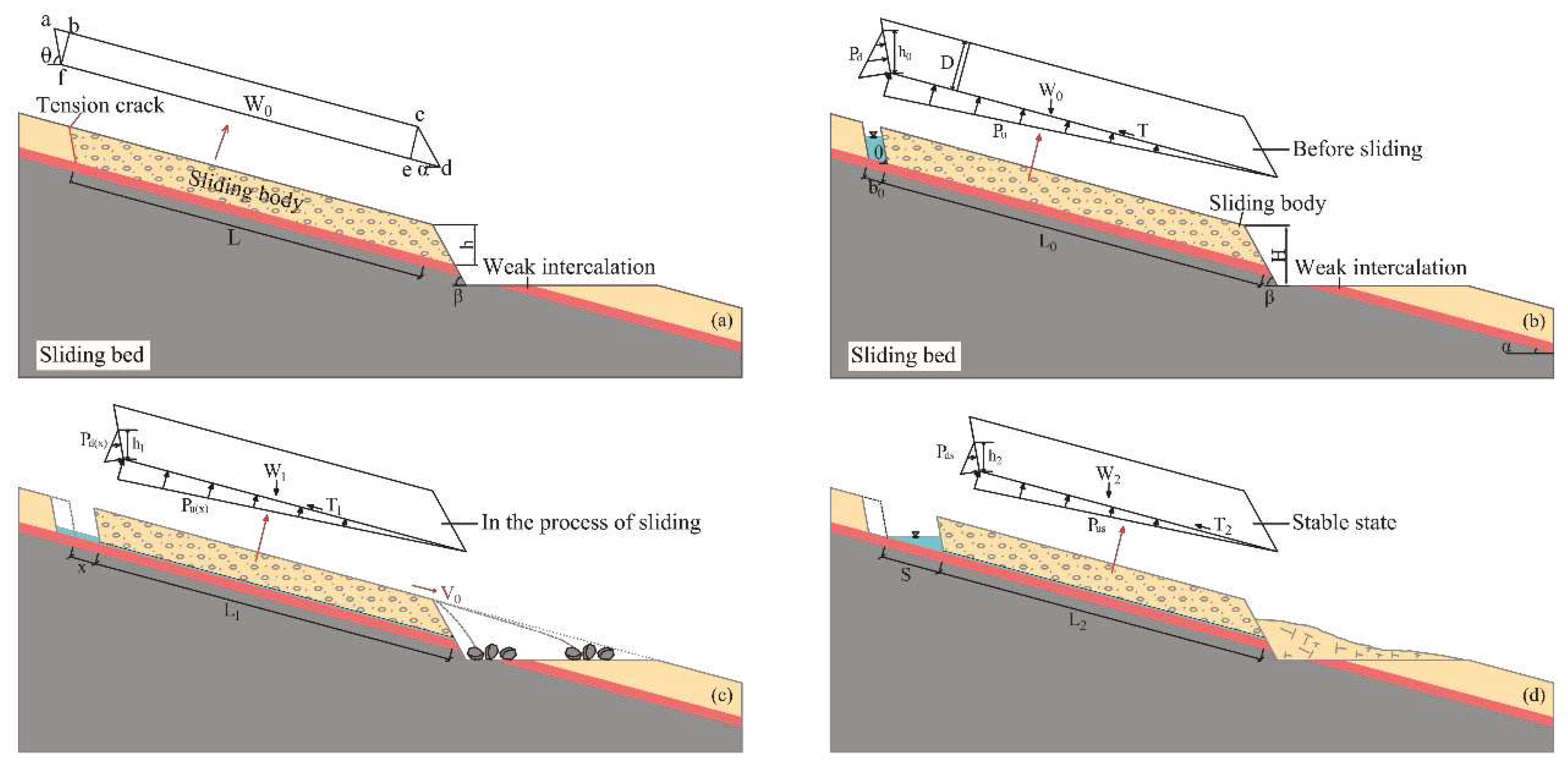
Without the influence of external forces, slopes tend to be steady over the long-term geological evolution process (Figure 1a). When road construction or open-pit mining is carried out, the stresses located around the slope are released, allowing them to readjust to the new state of balance, resulting in tension fractures around the rear margin (Figure 1b). As the project continues and rainfall occurs, the rear margin fractures expand, forming a tension crack, while surface water flows into the fractures, creating fracture water pressure and infiltration forces that cause the fractures to continue to expand in depth (Figure 1c). With the passage of time, after the fractures have expanded and connected, the overall landslide sliding force is greater than the resisting force, leading to the instability of the entire slope (Figure 1d) [49].

3.2. Mechanical analysis

Using the rigid body limit equilibrium method to derive the length of slope instability, the energy conservation theorem is employed to calculate the distance of slope movement.

3.2.1. Instability length

The excavation usually leads to local instability of the slope at the foot of the leading edge and tension cracks created at the trailing edge, which the state can be seen as understable at this time. Besides, the instability length calculated in this paper refers to the distance from the farthest crack at the trailing edge to the top of the excavated slope at the leading edge. A calculation model for instability length is developed based on a typical bedding rock slope (Figure 2a). By the limit equilibrium theory of rigid bodies:
K = R T = W 0 cos tan φ 0 + c 0 l d f + σ l a f W 0 sin
Where K denotes the stability coefficient, W0 stands for the weight of the sliding mass per unit width and represents the inclination angle of the rock stratum. l d f and l a f   indicates the length of df and af, while c0 and φ0 denote the cohesion and internal friction angle respectively. σ represents the equivalent tensile strength perpendicular to the af. W0 can be obtained from the following equation:
W 0 = S T γ = ( S cde + S abf + S bcef ) γ
Where ST represents the cross-sectional area of the sliding mass, and Scde, Sabf, and Sbcef are the areas of triangular cde, abf, and rectangular bcef, respectively. γ are the weight of the sliding body. Besides, assuming l e f =L, establish the side length relationship 3 to 5 from the geometric relationship:
l c d = h sin β , l c e = l c d sin ( β - ) = h sin ( β - ) sin β
l d e = l c d cos ( β - ) = h cos ( β - ) sin β , l ab = l bf tan ( θ - ) = h sin ( β - ) sin β tan ( θ - )
l af = h sin ( β - ) sin β cos ( θ - ) tan ( θ - ) , L 0 = l d f = l d e + l e f = h cos ( β - ) sin β + L
From equations 3-5, obtain the Scde, Sabf, and Sbcef
S c d e = l d e × l c e 2 = h 2 sin ( β - ) cos ( β - ) 2 sin 2 β
S a b f = l a b × l b f 2 = h 2 sin 2 ( β - ) 2 sin 2 β tan ( θ - )
S b c e f = l e f × l b f = Lh sin ( β - ) sin β
Substituting equations 6-8 into 2 yields:
W 0 = [ h 2 sin ( β - ) cos ( β - ) tan ( θ - ) + h 2 sin 2 ( β - ) + 2 L h sin β sin ( β - ) tan ( θ - ) ] γ 2 sin 2 β tan ( θ - )
substituting equations 9 into 1, and the following can be derived:
L ( γ h sin ( β - ) ( K sin - cos tan φ 0 ) sin β - c 0 ) = c 0 h cos ( β - ) sin β + σ hsin ( β - ) sin β cos ( θ - ) tan ( θ - ) - γ [ h 2 sin ( β - ) cos ( β - ) tan ( θ - ) + h 2 sin 2 ( β - ) ] ( K sin - cos tan φ 0 ) 2 sin 2 β tan ( θ - )
C o m m a n d   A = γ h sin ( β - ) ( K sin - cos tan φ 0 ) sin β
B = c 0 h cos ( β - ) sin β
D = σ hsin ( β - ) sin β cos ( θ - ) tan ( θ - )
M = γ [ h 2 sin ( β - ) cos ( β - ) tan ( θ - ) + h 2 sin 2 ( β - ) ] ( K sin - cos tan φ 0 ) 2 sin 2 β tan ( θ - )
Substituting equations 11 through 14 into 10 results in:
L = B + D M A c 0
Getting the final instability length l a c :
l a c = L + l a b = B + D M A c 0 + h sin ( β - ) sin β tan ( θ - )
Where β is the slope excavation angle, θ represents the angle between the trailing edge crack and the horizontal plane. Additionally, h refers to the excavation height of the sliding mass.

3.2.2. Runout distance

The calculation model for slope instability to stability, divided into three stages (I~III), is illustrated in Figure 2b-2d. The water head heights of the trailing edge fractures in stages II and III are represented by h1 and h2 respectively, while the lengths of the bottom surface of the sliding mass along the sliding direction in the latter two stages are denoted by L1 and L2. W1 and W2 refer to the unit width weight of the slope in the aforementioned stages, and b0 represents the length of the fracture along the sliding surface prior to slope instability. H stands for the excavation height, x denotes the distance traveled by the sliding mass on the slope, and d is the average thickness of the sliding body. V0 represents the speed at which the sliding mass moves at distance x, while G denotes the moving distance of the sliding body on the slope in stage III.
During intense rainfall conditions, a considerable amount of rainwater infiltrates the tension cracks at the trailing edge, creating hydrostatic pressure. Furthermore, water infiltration induces uplift pressure along the sliding surface. During landslide motion, four forces should be considered: self-gravity W1, anti-sliding force f1, hydrostatic pressure Pd (x), and uplift pressure Pu (x). Additionally, the sliding mass decreases continually during the movement owing to the formation of a free face resulting from front edge excavation, and result in these forces undergo constant changes during stage II, which is distinct from the scenario where the impact of excavation factors is not taken into account.
Assuming that the volume of water in the cracks at the rear edge of the landslide remains constant, and θ is nearly vertical. The water-filled cross-sectional areas s0 and s1 in the cracks during the I and II stages can be expressed by Equations 17 and 18, respectively:
s 0 = b 0 sin ( θ ) ( 2 h 0 b 0 cos ( θ ) ) 2
s 1 = h 1 ( b 0 + x ) sin ( θ )
When s0=s1, the relationship between h0 and h1 and the motion distance x can be expressed as follows:
h 1 = b 0 ( 2 h 0 b 0 cos ( θ ) ) b 0 + x
Set N= b 0 ( 2 h 0 b 0 cos ( θ ) ) ,So h 1 = N / ( b 0 + x ) .
The relationship between W0, W1, and x can be expressed:
W 1 = W 0 ( L 0 x ) L 0
The relationships among L0, L1, and L2 are established through the following equations:
L 1 = L 0 x L 2 = L 0 G
In the II stage, Equation 22 depicts the hydrostatic pressure Pd (x) and the uplift pressure Pu (x). The hydrostatic pressure Pd (x) can be divided into two forces, namely a parallel force Pd1 (x) and a perpendicular force Pd2 (x), as illustrated in Equation 23. Additionally, the anti-sliding force f1 is as shown in Equation 24:
P d ( x ) = γ w h 1 2 2 , P u ( x ) = γ w h 1 ( L 0 x ) 2
P d 1 ( x ) = γ w h 1 2 sin ( θ ) 2 , P d 2 ( x ) = γ w h 1 2 cos ( θ ) 2
f 1 = ( W 1 cos γ w h 1 ( L 0 x ) 2 γ w h 1 2 cos ( θ ) 2 ) tan φ 0 + c o L 1
The shear strength parameter of the sliding belt in Equation 24 should be the residual strength parameter.
Assuming that the sliding mass comes to a halt at a distance of G on the slope. The kinetic energy of the landslide when it moves a distance x (0<x<G) is determined by two parts: the gravitational potential energy required to overcome resistance and the hydrostatic pressure that performs work. Therefore, the law of energy conservation can be applied to derive the following equation:
m 1 v 0 2 2 = W G W f 1 + W p d ( x )
In Equation 26-29, m1 represents the mass of the sliding body at a given moving distance x. WG denotes the work that is accomplished by the gravity of the sliding mass during this movement. Additionally, Wf1 represents the work that is done by the anti-sliding force, while Wpd(x) refers to the work that is accomplished by the hydrostatic pressure at the trailing edge. The details are as follows:
m 1 = W 1 / g
W G = 0 x W 1 sin d x
W f 1 = 0 x f 1 d x
W pd ( x ) = = 0 x P d 1 ( x ) d x
Where g represents the acceleration of gravity, by substituting Equation 20 into 27, we can obtain WG:
W G = W 0 x sin W 0 x 2 sin 2 L 0
By substituting Equations 20, 23, and 24 into 28 and 29, we obtain the following expressions for Wf1 and Wpd(x):
W f 1 = W 0 cos tan φ 0 ( x x 2 2 L 0 ) + ( γ w N tan φ 0 [ x ( b 0 + L 0 ) I n ( b 0 + x b 0 ) ] ) / 2 + γ w N 2 tan φ 0 cos ( θ ) 2 ( b 0 + x ) γ w N 2 tan φ 0 cos ( θ ) 2 b 0 + c 0 L 0 x c 0 x 2 2
W p d ( x ) = γ w K 2 sin ( θ ) 2 b 0 γ w K 2 sin ( θ ) 2 ( b 0 + x )
Substituting Equations 30 to 32 into 25 yields:
m 1 v 0 2 2 = W 0 x sin W 0 x 2 sin 2 L 0 ( γ w N tan φ 0 [ x ( b 0 + L 0 ) I n ( b 0 + x b 0 ) ] ) / 2 W 0 cos tan φ 0 ( x x 2 2 L 0 ) c 0 L 0 x + c 0 x 2 2 + γ w N 2 ( sin ( θ ) + tan φ 0 cos ( θ ) ) 2 b 0 γ w N 2 ( sin ( θ ) + tan φ 0 cos ( θ ) ) 2 ( b 0 + x )
Order I= sin ( θ ) + tan φ 0 cos ( θ ) , and V0 can be expressed:
v 0 = { 2 g L 0 x sin g cos tan φ 0 ( 2 L 0 x x 2 ) g x 2 sin L 0 x + g L 0 c 0 ( x 2 2 L 0 x ) W 0 ( L 0 x ) γ w g L 0 N tan φ 0 [ x ( b 0 + L 0 ) I n ( b 0 + x b 0 ) ] W 0 ( L 0 x ) + γ w g N 2 L 0 I W 0 b 0 ( L 0 x ) γ w g N 2 L 0 I W 0 ( L 0 x ) ( b 0 + x ) } 1 2
When the moving distance reach G, in accordance with the principle of energy conservation:
W f 1 = W G + W p d ( x )
Substitute x=G into Equation 35 to obtain:
W 0 cos tan φ 0 ( G G 2 2 L 0 ) + ( γ w N tan φ 0 [ G ( b 0 + L 0 ) I n ( b 0 + G b 0 ) ] ) / 2 + γ w N 2 tan φ 0 cos ( θ ) 2 ( b 0 + G ) γ w N 2 tan φ 0 cos ( θ ) 2 b 0 + c 0 L 0 G c 0 G 2 2 = W 0 G sin W 0 G 2 sin 2 L 0 + γ w N 2 sin ( θ ) 2 b 0 γ w N 2 sin ( θ ) 2 ( b 0 + G )
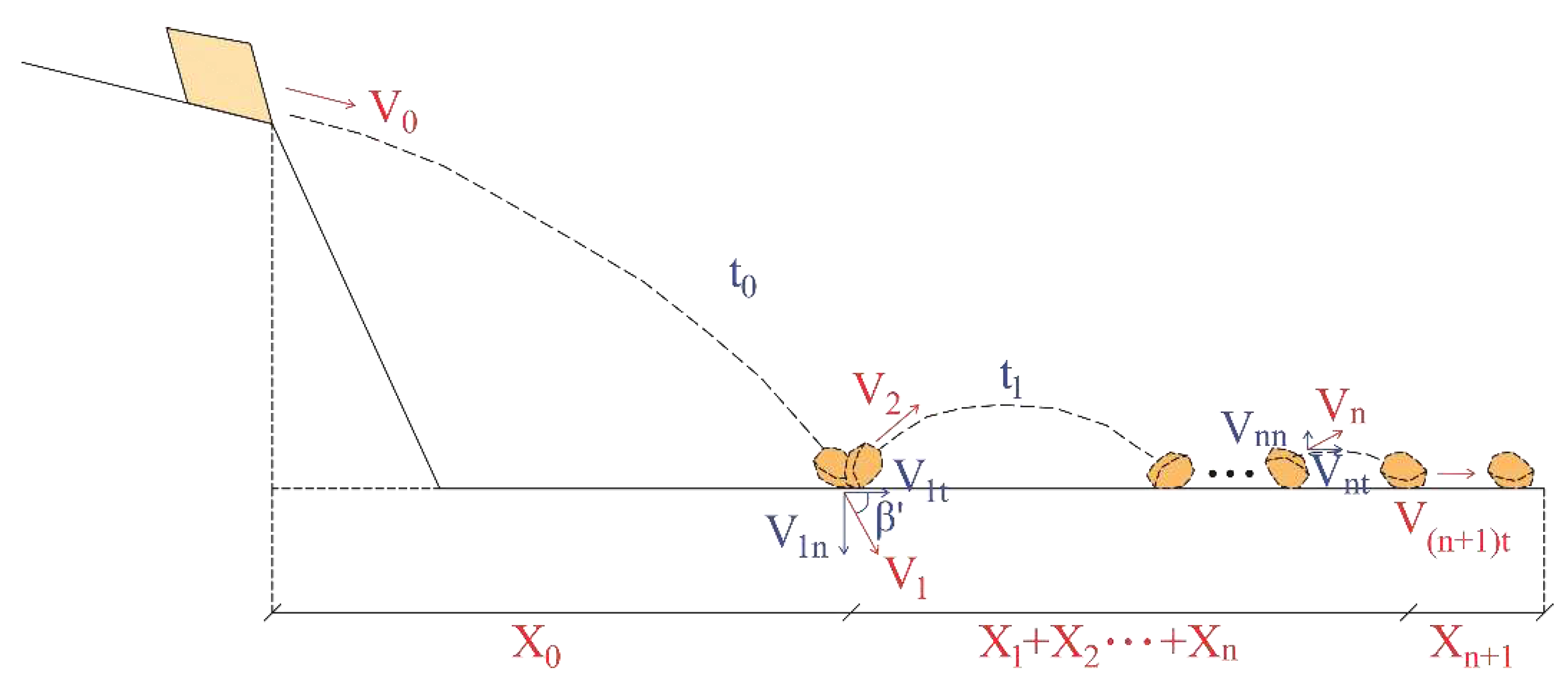
G can be calculated using Equation 36, with relevant parameters derived from real scenarios. The total displacement of a landslide comprises three components. Firstly, the horizontal distance X0 covered by the slider during its initial movement in the air. Secondly, the horizontal displacement X1+... Xn of the sliding body as it collides with the ground repeatedly (assuming n collisions) until its normal velocity reaches 0. Lastly, there is the displacement Xn+1 generated by the block sliding on the ground, as depicted in Figure 3.
Command Y= H d 2 sin ( θ ) ,we can obtain:
V 0 sin ( ) t 0 + gt 0 2 2 = Y ,   X 0 = V 0 cos ( ) t 0 ,   m 1 V 1 2 2 = m 1 V 0 2 2 + m 1 g Y
T0, X0, and V1 can be expressed as:
t 0 = ( V 0 2 sin 2 + 2 g Y ) 1 2 V 0 sin g
X 0 = V 0 cos [ ( V 0 2 sin 2 + 2 g Y ) 1 2 V 0 sin ] g , V 1 = V 0 2 + 2 g Y
When a block collides with the ground at a velocity of V1, the incomplete elastic collision results in a loss of energy and a decrease in the block's velocity. To describe this phenomenon, we introduce the normal restitution coefficient R1n and the tangential restitution coefficient R1t. The relationship between the initial normal velocity V1n and tangential velocity V1t of the block prior to the collision, and the resulting normal velocity V2n and tangential velocity V2t of the block after the collision can be expressed as follows:
V 2 n = V 1 n R 1 n , V 2 t = V 1 t R 1 t
V1n and V1t can be expressed:
V 1 n = V 1 sin β ' V 1 t = V 1 cos β ' tan β = V 0 sin + gt 0 V 0 cos β = arctan ( V 0 sin + gt 0 V 0 cos )
Where β ' is the angle between V1 and the horizontal plane (Figure 3):
X1 represents the movement distance of the block between the first collision and the second collision, which can be expressed as following:
X 1 = V 2 t t 1 t 1 = 2 V 2 n g
Further, X1 can be described as:
X 1 = 2 R 1 n R 1 t V 1 n V 1 t g
Similarly, X2 … Xn can be expressed as:
X 2 = 2 R 1 n 2 R 1 t 2 V 1 n V 1 t g , X n = 2 R 1 n n R 1 t n V 1 n V 1 t g
The second part of the movement distance can be calculated as following:
X 1 + X 2 + + X n = 2 R 1 n R 1 t V 1 n V 1 t g + 2 R 1 n 2 R 1 t 2 V 1 n V 1 t g + + 2 R 1 n n R 1 t n V 1 n V 1 t g = 2 V 1 n V 1 t R 1 n R 1 t [ 1 - ( R 1 n n R 1 t n ) ] g ( 1 - R 1 n R 1 t )
At the n+1 collision, the normal velocity of the block attenuates to 0, and the block slides on the ground at a velocity of V (n+1) t, and the associated motion equation can obtain:
V ( n + 1 ) t = V 1 t R 1 t n , m 1 V ( n + 1 ) t 2 2 = μ m 1 g X n + 1
The third stage movement distance Xn+1 can be expressed as:
X n + 1 = V ( n + 1 ) t 2 2 μ g = V 1 t 2 R 1 t 2 n 2 μ g
The final runout distance Xt of the landslide can be gained as follows:
X t = V 0 cos [ V 0 2 sin 2 + 2 g Y V 0 sin ] g + 2 V 1 n V 1 t R 1 n R 1 t [ 1 - ( R 1 n n R 1 t n ) ] g ( 1 - R 1 n R 1 t ) + V 1 t 2 R 1 t 2 n 2 μ g
Substituting Equation 38 and 40 into 47 yields:
X t = V 0 cos [ V 0 2 sin 2 + 2 g Y V 0 sin ] g + 2 ( V 0 2 + 2 g Y ) s i n β ' cos β ' R 1 n R 1 t [ 1 - ( R 1 n n R 1 t n ) ] g ( 1 - R 1 n R 1 t ) + ( V 0 2 + 2 g Y ) cos β ' R 1 t 2 n 2 μ g
Generally speaking, the velocity of landslide will undergoes an initial increase until reach maximum followed by a subsequent decrease. The maximum speed occurs when the anti sliding force equals the sliding force once again, and can be expressed:
f 1 = P d 1 ( x ) + W 1 sin
49 can be written as:
( W 1 cos γ w h 1 ( L 0 x ) 2 γ w h 1 2 cos ( θ ) 2 ) tan φ 0 + c o L 1 = γ w h 1 2 sin ( θ ) 2 + W 1 sin
Eventually available:
W 0 ( L 0 G 0 ) ( cos tan φ 0 sin ) L 0 γ w N tan φ 0 ( L 0 G 0 ) 2 ( b 0 + G 0 ) + c o ( L 0 G 0 ) = γ w N 2 ( cos ( θ ) tan φ 0 + sin ( θ ) ) 2 ( b 0 + G 0 ) 2
Where G0 represent the movement distance of the sliding mass on the slope when the block speed reaches the maximum, which can be obtained by substituting the relevant parameters into Equation 51, and Vmax of the sliding mass on the slope can be obtained as follows:
v max = { 2 g L 0 G 0 sin g cos tan φ 0 ( 2 L 0 G 0 G 0 2 ) g G 0 2 sin L 0 G 0 + g L 0 c 0 ( G 0 2 2 L 0 G 0 ) W 0 ( L 0 G 0 ) γ w g L 0 N tan φ 0 [ G 0 ( b 0 + L 0 ) I n ( b 0 + G 0 b 0 ) ] W 0 ( L 0 G 0 ) + γ w g N 2 L 0 N W 0 b 0 ( L 0 G 0 ) γ w g N 2 L 0 I W 0 ( L 0 G 0 ) ( b 0 + S 0 ) } 1 2
Moreover, given the monotonically increasing correlation between Xt and V, the ultimate displacement distance Xt of the landslide can be formulated as follows:
X t = V max cos [ V max 2 sin 2 + 2 g Y V max sin ] g + 2 ( V max 2 + 2 g Y ) s i n β ' cos β ' R 1 n R 1 t [ 1 - ( R 1 n n R 1 t n ) ] g ( 1 - R 1 n R 1 t ) + ( V max 2 + 2 g Y ) cos β ' R 1 t 2 n 2 μ g

4. Case verification

Taking Xinjianan landslide as an example, the feasibility of the model is verified through case analysis and numerical simulation.
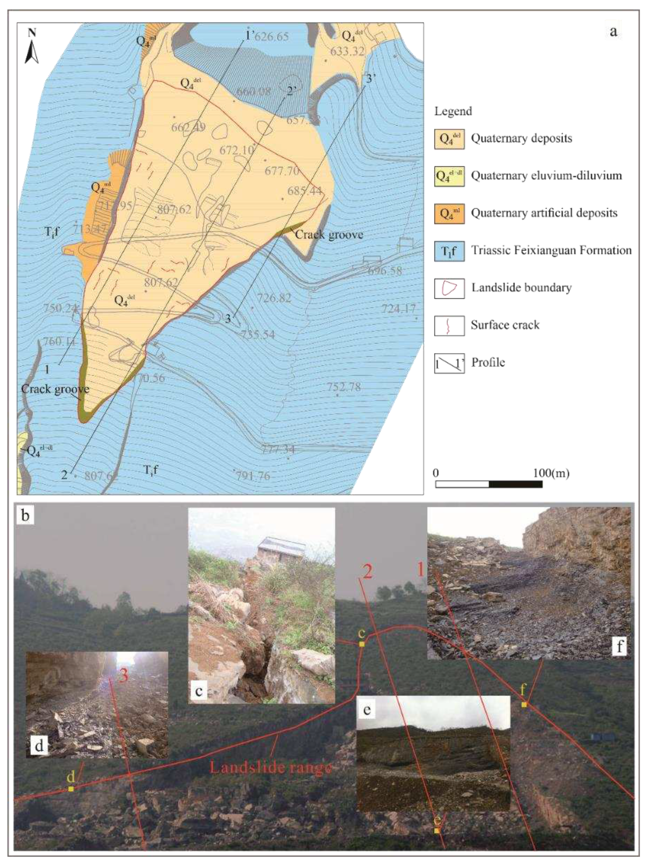
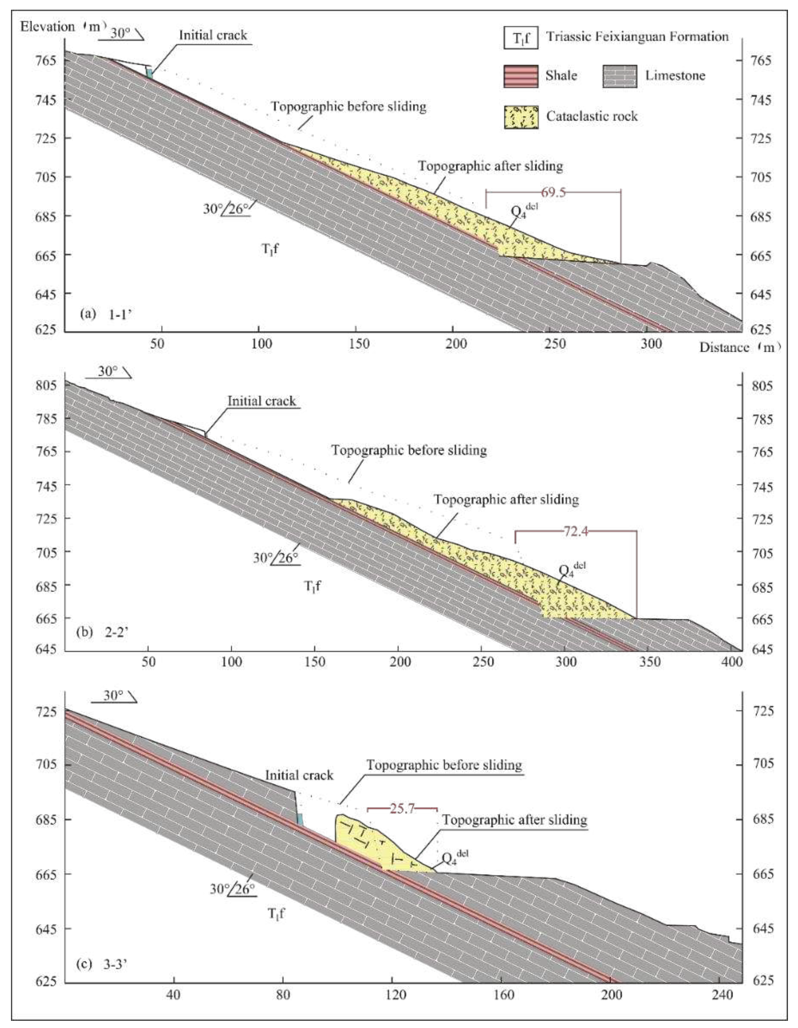
The landslide is located in Dongcheng Office, Nanchuan District, Chongqing. At 8:00 pm on December 27, 2012, a bedding slide with a volume of approximately 24.06 × 10⁴ m3 occurred on the slope. The landslide exhibits a longitudinal extent of approximately 304 m, an average width of roughly 106 m, and a thickness ranging from 2.5 to 30.0 m. Its primary sliding direction is approximately 30 ° (Figures 4a, 4b). The sliding mass primarily comprises cataclastic rock mass, with limestone and shale composing the lithology. Besides, the slip zone is a weak interlayer containing shale, while the sliding bed is composed of limestone from the Feixianguan Formation of the Triassic System, with a rock occurrence of 30 °∠ 26 °. The leading edge of the landslide underwent excavation as a result of open-pit mining, reaching a height range of 9.2 to 42.6 m (Figure 4e). Specifically, the front edge of the 1-1 'to 3-3' profile was excavated at varying heights of 28 m, 42.6 m, and 21.7 m, respectively (Figure 5). Prior to the onset of slope instability, tensile cracks measuring between 0.5 and 2.5 meters in width were observed along the rear edge (Figure 4c), northeast front edge, and middle of the west boundary. Following the instability event, the tensile fracture groove widened, with the rock mass structure appearing to be most intact along section 3-3' (Figure 4d), followed by section 2-2', while section 1-1' exhibited the most pronounced fracturing (Figure 4f).

4.1. Case analysis

Utilizing the outcomes of on-site investigations, survey reports, and records documented by on-site patrol personnel, the calculation parameters for each section were obtained. The strength paramaters of the sliding zone soil was determined through indoor direct shear tests, with c0, φ 0 at 13.5 kN/m2, 9.5° respectively. Considering that the excavation platform serves as a road following its construction, reference was made to the findings of Zhang et al. [50] (Table 1) to ascertain that R1n and R1t are 0.4 and 0.87, respectively. Following seven collisions, the normal velocity was only 0.16% of the speed before the initial collision, can take for its impact negligible. The number of collisions, n, was set at 7. The sliding friction coefficient was determined as 0.58, based on the results of Huang et al. [51], and the numerical values of other parameters are presented in Table 1.
Substituting the above parameters into Eqs. 18, 54 and 55 gives the results of the FEL and movement distance. The outcome were then compared with the real results (Table 2).
Where l a c and l a c ' represent the FEL derived from theoretical calculations and on-site measurements, while Xt and Xt’ denote the displacement distances obtained from calculations and surveys.
Based on the findings, it is evident that the FEL obtained from the calculation is smaller than the actual, whereas the moving distance from computing is larger. Nevertheless, the error is within 20%, which is deemed acceptable, proving that these methods possess some degree of practical applicability.

4.2. Numerical simulation analysis

Two types of environmental scenarios were therefore considered: 1) excavation, 2) excavation + hydrostatic pressure.

4.2.1. Model implementation and parameter determination

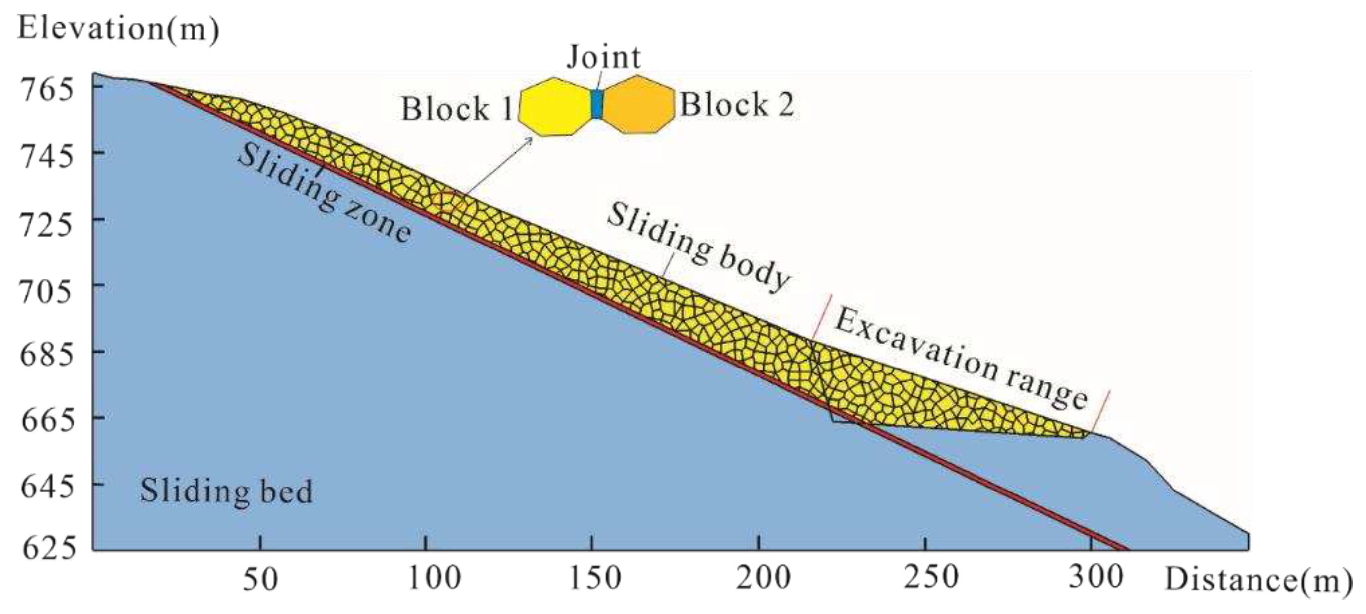
A two-dimensional model (Figure 6) is developed considering a vertical cross-section (Profile 1 in Figure 4a) oriented SW-NE that is perpendicular to the topographic surface. This cross-section extends from the slope crest (770 m) to the slope base (659 m). The slide material, as stated above in Section 4.1, is composed mainly of rubble, represented by blocks in the model, and silty clay, which is treated as the joint between these rock blocks that bonds them together (Figure 4a). Field investigations revealed that the slope base is dominated by layered bedrocks. The model is constrained by displacement-type boundary conditions: no bottom vertical displacement and no horizontal displacement at the left side are permitted. In this case, rigid blocks are assumed whereas the joints are assumed to behave according to an elastoplastic law with the Mohr-Coulomb failure criterion. Besides, since the sliding mass consists of cataclastic rock, which shape is inherently uncertain, and can be delineated using Voronoi.
To accurately reconstruct the damage behavior using inversion, the primary parameters and boundary conditions are established as follows:
1. The strength parameters of both the slip zone and slip body are initially set to their peak strength until tension cracks emerge at the trailing edge. Subsequently, the strength parameters of the slip zone and slip body are set to their residual strength.
2. Once tension cracks appear at the trailing edge of the slip body, hydrostatic pressure is applied along the rupture surface of both the trailing edge and substrate.
The materia properties of landslide are shown in Table 3, and the mechanical characteristics of the matrix and joints properties assigned to the joint network are listed in Table 4. These parameters were initially acquired from in indoor experiments and relevant literature [52,53,54]. Afterward, via inverse analysis until appropriate parameters are obtained to predict the possible kinematic evolution of the landslide in different cases.

4.2.2. Result of numerical tests

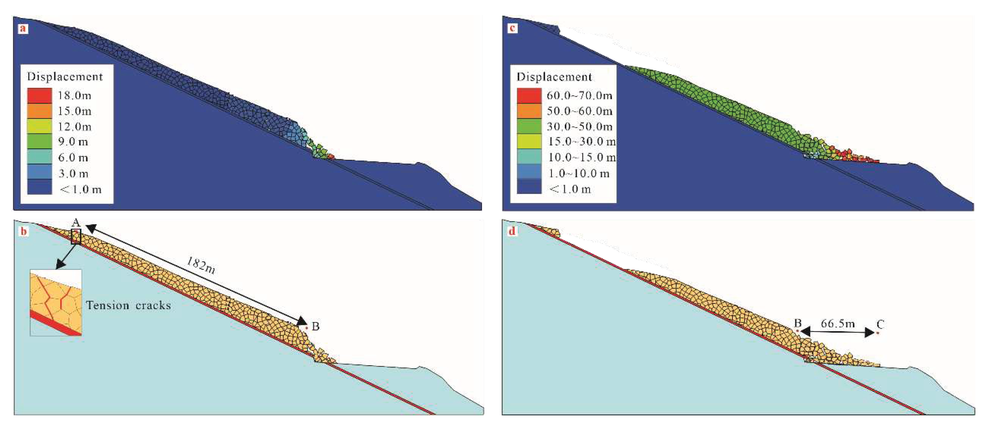
Considering the excavation conditions alone, partial slope damage occurs primarily at the front edge, resulting in block stones rolling off up to a distance of approximately 18m (Figure 7a). Besides, tension cracks appear at the rear edge, with the maximum distance of approximately 182 m from the front edge (Figure 7b). However, because of cracks at the trailing edge, once encounter continuous rainfall, will lead to a rapid decrease in the strength parameters of the sliding mass and sliding zone. In this scenario, hydraulic conditions and parameter weakening should be considered. Therefore, hydrostatic pressure was applied along the trailing edge cracks and weak layers of the landslide then, and the parameters were set as residual strength parameters. The final results are shown in Figures 7c and 7d. The outcome is an overall slope failure with a maximum movement distance of approximately 66.5m (Figure 7c, 7d), which is in good agreement with the theoretical model conclusion.

5. Discussion

The theoretical framework presented in this paper primarily pertains to sliding-tensile translational rockslides belongs to overall destruction, typically characterized by inclination angles ranging from 20 to 30°. However, given the variability of landslide parameters and intricate internal dynamics, it is inadvisable to rely solely on this model for determining instability length and movement distance during slope design. Instead, integrating the theoretical calculations with numerical simulations can yield more robust outcomes.

6. Conclusion

The paper presents an analysis of the instability behavior of translational rockslide under excavation conditions, focusing on two critical parameters: slope instability length and post-damage movement distance. A theoretical model for these parameters is proposed based on the principles of limit equilibrium of rigid bodies and conservation of momentum. The feasibility of this model is demonstrated through example verification and numerical simulations.
Under excavation conditions, the translational rock slope typically induces localized damage at the leading edge and tension cracks at the trailing edge. Subsequent rainfall is the primary factor contributing to the overall damage of these slopes, which is consistent with the findings of numerical simulations.
The theoretical model presented in this paper exhibits certain discrepancies with the actual system, which is mainly attributed to the uncertainties in strength parameters and the deviations in geometric parameter estimations. Specifically, the calculated instability length is smaller than the actual value, while the movement distance is larger. Therefore, it is recommended to integrate the theoretical model with numerical simulations to determine these two critical parameters in slope engineering design and risk assessment.

Data Availability Statement

Not applicable.

Acknowledgments

This work is supported by the National Natural Science Foundation of China (Nos. 42077277), and Youth Science Foundation (Nos. 42107160).

References

  1. Wu, Lili, et al. "Research on the excavation stability evaluation method of Chaqishan ancient landslide in China." Engineering Failure Analysis 2022, 141, 106664. [CrossRef]
  2. Y. Togashi, K.Y. Togashi, K. Mizuo; et al. Evaluating Changes in the Degree of Saturation in Excavation Disturbed Zones Using a Stochastic Differential Equation. Computers and Geotechnics 2022, 143. [Google Scholar] [CrossRef]
  3. T. Liu, Y. Xie, Z.H. Feng; et al. Better Understanding the Failure Modes of Tunnels Excavated in the Boulder-Cobble Mixed Strata by Distinct Element Method. Engineering Failure Analysis 2020, 116, 104712. [Google Scholar] [CrossRef]
  4. S.S. Xu, H. Lei, C. Li; et al. Model Test on Mechanical Characteristics of Shallow Tunnel Excavation Failure in Gully Topography. Engineering Failure Analysis 2021, 119, 104978. [Google Scholar] [CrossRef]
  5. B. Bayer, A. Simoni, D. Schmidt. Using Advanced InSAR Techniques to Monitor Landslide Deformations Induced by Tunneling in the Northern Apennines Italy. Engineering Geology 2017, 226, 20–32. [Google Scholar] [CrossRef]
  6. Guo, Changbao, et al.; et al. Study of an ancient landslide reactivation mechanism based on centrifuge model testing: an example of the Jiangdingya ancient landslide reactivation in 2018, Gansu Province, China. Landslides 2023, 20, 127–141. [Google Scholar] [CrossRef]
  7. Zhang, Chonglei, et al; et al. Large-scale shaking table test on seismic behaviour of anti-slide pile-reinforced bridge foundation and gravel landslide: a case study. Bulletin of Engineering Geology and the Environment 2021, 80, 1303–1316. [Google Scholar] [CrossRef]
  8. Guo, Jian, et al.; et al. The effect of topography on landslide kinematics: a case study of the Jichang town landslide in Guizhou, China. Landslides 2020, 17, 959–973. [Google Scholar] [CrossRef]
  9. E. Botero, E. Ovando, M.J. Mendoza. Successful prediction of slope failure in an excavation trial. Engineering Failure Analysis. 2020, 109, 104392. [Google Scholar] [CrossRef]
  10. K.R. Praveen, J. Chophel, J. Wangchuk; et al. IBIS-FM Radar as A Tool for Monitoring Hill Slopes During Excavations in Hydropower Projects: A Case Study from Bhutan Himalayas. Energy Geoscience. 2021; 1–7. [Google Scholar] [CrossRef]
  11. F. Florin, L. Maria, D. Ciprian. IzabelaMaria, Investigations on the Stability of the Right Slope in the Area of Anina Wastewater Treatment Plant, Revista Minelor / Mining Revue. 2022, 27, 7–18. [Google Scholar] [CrossRef]
  12. Du J, Shi X, Chai B; et al. Force and energy equilibrium-based analytical method for progressive failure analysis of translational rockslides: formulation and comparative study. Landslides 2023, 20, 475–488. [Google Scholar] [CrossRef]
  13. Wang W, Song H, Zhang Z; et al. Landslide Multi-attitude Data Measurement of Bedding Rock Slope Model[J]. International Journal of Parallel Programming 2020, 48, 928–939. [Google Scholar] [CrossRef]
  14. Peng Y, Dong S, Lu Z; et al. A method for calculating permanent displacement of seismic-induced bedding rock landslide considering the deterioration of the structural plane. Frontiers in Earth Science, 2023; 2272. [Google Scholar] [CrossRef]
  15. Dai Z, Zhang L, Wang Y; et al. Deformation and failure response characteristics and stability analysis of bedding rock slope after underground adverse slope mining. Bulletin of Engineering Geology and the Environment 2021, 80, 4405–4422. [Google Scholar] [CrossRef]
  16. Yu, X., Gong. Study of the slope deformation characteristics and landslide mechanisms under alternating excavation and rainfall disturbance. Bull Eng Geol Environ 2021, 80, 7171–7191. [Google Scholar] [CrossRef]
  17. Wang J Y, Li L, Zheng D G, et a1. Characteristics of Apparent Dip Slide and Movement Process of the "8.12" Shanyang Rockslide. Journal of Catastrophology (in Chinese with English abstract). 2018, 33, 111–116. [CrossRef]
  18. Zhu X, Xie L, Tang Y; et al. Progressive Formation of Retrogressive Landslide and the Lateral Length of Instability. Applied Sciences 2023, 13, 799. [Google Scholar] [CrossRef]
  19. Li J, Chen S, Yu F; et al. Reinforcement mechanism and optimisation of reinforcement approach of a high and steep slope using prestressed anchor cables. Applied Sciences 2019, 10, 266. [Google Scholar] [CrossRef]
  20. Liu Z, Qiu H, Ma S; et al. Surface displacement and topographic change analysis of the Changhe landslide on September 14, 2019, China. Landslides 2021, 18, 1471–1483. [Google Scholar] [CrossRef]
  21. Johari A, Mousavi S. An analytical probabilistic analysis of slopes based on limit equilibrium methods. Bulletin of Engineering Geology and the Environment 2019, 78, 4333–4347. [Google Scholar] [CrossRef]
  22. Cheng H, Zhou X. A novel displacement-based rigorous limit equilibrium method for three-dimensional landslide stability analysis. Can Geotech J 2015, 52, 2055–2066. [Google Scholar] [CrossRef]
  23. Zhou XP, Cheng H. Analysis of stability of three-dimensional slopes using the rigorous limit equilibrium method. Eng Geol 2013, 160, 21–33. [Google Scholar] [CrossRef]
  24. Sengani F, Allopi D. Accuracy of Two-Dimensional Limit Equilibrium Methods in Predicting Stability of Homogenous Road-Cut Slopes. Sustainability 2022, 14, 3872. [Google Scholar] [CrossRef]
  25. Feng J, Zhou D P, Jiang N. On the Extent of Bedding Slipping Rockmass of Consequent Rock Slope. Journal of Mountain Science (In Chinese with English abstract). 2007, 3, 376–380. [Google Scholar]
  26. Deng R G, Zhou D P, Li A H; et al. On the Critical Length of Unstable Rock Stratum on bedrock slope. Chinese Journal of Geotechnical Engineering (in Chinese with English abstract). 2002, 24, 178–181. [Google Scholar]
  27. Su X, Wei W, Ye W; et al. Predicting landslide sliding distance based on energy dissipation and mass point kinematics. Natural Hazards 2019, 96, 1367–1385. [Google Scholar] [CrossRef]
  28. Hattanji T, Moriwaki H. Morphometric analysis of relic landslides using detailed landslide distribution maps: implications for forecasting travel distance of future landslides. Geomorphology 2009, 103, 447–454. [Google Scholar] [CrossRef]
  29. Guo D P, Hamada M, He C. An empirical model for landslide travel distance prediction in Wenchuan earthquake area. Landslides 2014, 11, 281–291. [Google Scholar] [CrossRef]
  30. Guo C B, Zhang Y S, Montgomery D R; et al. How unusual is the long-runout of the earthquake-triggered giant Luanshibao landslide, Tibetan Plateau, China? Geomorphology 2016, 259, 145–154. [Google Scholar] [CrossRef]
  31. Hungr, O. A model for the runout analysis of rapid flow slides, debris flows, and avalanches. Can Geotech J 1995, 32, 610–623. [Google Scholar] [CrossRef]
  32. Miao T D, Liu Z Y, Niu Y H. A sliding block model for the runout prediction of high-speed landslides. Can Geotech J 2001, 38, 217–226. [Google Scholar] [CrossRef]
  33. Wang J D, Xiao S F, Zhang Z Y. The mechanism for movement of irrigation-induced high-speed loess landslide. J Eng Geol (In Chinese with English abstract). 2001, 9, 241–246. [Google Scholar]
  34. He S M, Liu W, Wang J. Dynamic simulation of landslide based on thermo-poroelastic approach. Comput. Geosci. 2015, 75, 24–32. [Google Scholar] [CrossRef]
  35. Scaringi G, Fan X, Xu Q; et al. Some considerations on the use of numerical methods to simulate past landslides and possible new failures: the case of the recent Xinmo landslide (Sichuan, China). Landslides 2018, 15, 1359–1375. [Google Scholar] [CrossRef]
  36. Huang Y, Li G, Xiong M. Stochastic assessment of slope failure run-out triggered by earthquake ground motion. Nat. Hazards 2020, 101, 87–102. [Google Scholar] [CrossRef]
  37. Mitchell A, McDougall S, Nolde N; et al. Rock avalanche runout prediction using stochastic analysis of a regional dataset. Landslides 2020, 17, 777–792. [Google Scholar] [CrossRef]
  38. Zhang Z, Zeng R, Meng X; et al. Estimating landslide sliding distance based on an improved Heim sled model. Catena 2021, 204, 105401. [Google Scholar] [CrossRef]
  39. Jiang P, Chen J J. Displacement prediction of landslide based on generalized regression neural networks with K -fold cross-validation. Neurocoputing 2016, 198, 40–47. [Google Scholar] [CrossRef]
  40. Liu Y, Xu C, Huang B; et al. Landslide displacement prediction based on multi-source data fusion and sensitivity states. Engineering Geology. 2020, 271, 105608. [Google Scholar] [CrossRef]
  41. Li X, Tang X, Zhao S; et al. MPM evaluation of the dynamic runout process of the giant Daguangbao landslide. Landslides 2021, 18, 1509–1518. [Google Scholar] [CrossRef]
  42. Zhang C, Yin Y, Yan H; et al. Centrifuge modeling of multi-row stabilizing piles reinforced reservoir landslide with different row spacings. Landslides 2022, 20, 559–577. [Google Scholar] [CrossRef]
  43. Zhou C, Cao Y, Yin K; et al. Characteristic comparison of seepage-driven and buoyancy-driven landslides in Three Gorges Reservoir area, China. Engineering Geology 2022, 301, 106590. [Google Scholar] [CrossRef]
  44. Ge Y F, Tang H M, Li Wei; et al. Evaluation for Deposit Areas of Rock Avalanche Based on Features of Rock Mass Structure. Earth Science (In Chinese with English abstract). 2016, 41, 1583–1592. [Google Scholar]
  45. Dai X R, Zhao J J, Lai Q Y; et al. Movement Process and Formation Mechanism of Rock Avalanche in Chada, Tibet Plateau. Earth Science. (In Chinese with English abstract). 2022, 47, 1932–1944. [Google Scholar] [CrossRef]
  46. Tang R, Xu Q, Wu B; et al. Method of sliding distance calculation for translational landslides. Rock and Soil Mechanics. (In Chinese with English abstract). 2017, 39, 1009–1019+1070. [Google Scholar]
  47. Yang L, Wang Y, Zhang Q et al.; et al. A theoretical model about runout distance of bedding rock landslide under excavation uploading [J/OL]. Earth Science:1-15[2023-06-05]. Available online: http://kns.cnki.net/kcms/detail/42.1874.P.20230-420.1013.002.html.
  48. Itasca, 2004. UDEC Version 4.0 Universal Distinct Element Code. Itasca Consulting Group, Inc.
  49. Li X M, Yan E C, YanY; et al. Deformation Zoning and Treatment of a Toppling Deformation Slope Beside the Diversion Channel of a Hydropower Station. Bulletin of Geological Science and Technology (In Chinese with English abstract). 2019, 38, 227–235. [Google Scholar]
  50. Mu C, L. 2017. Study on deformation instability evolution mechanism and prediction during excavating process of bedded rock slope - A case of slope as the studied object in the Gasoline construction site. Doctoral dissertation. Chengdu University of Technology.
  51. Zhang Y H, Zhang M X, Cheng Q. Kinematics analysis for calculating distance of rockfalls on typical loose media slope. Journal Of ShangHai University (Natural Science). 2017, 23, 949–960. [Google Scholar] [CrossRef]
  52. Huang R Q, Liu W H. Study on the movement characteristics of rolling rock blocks on platform. Advances in Earth Science. (In Chinese with English abstract). 2008, 5, 517–523. [Google Scholar]
  53. Huang D, Gu D M, Song Y X; et al. Towards a complete understanding of the triggering mechanism of a large reactivated landslide in the Three Gorges Reservoir. Engineering Geology 2018, 238, 36–51. [Google Scholar] [CrossRef]
  54. Guglielmi Y, Cappa F, Binet S. Coupling between hydrogeology and deformation of mountainous rock slopes: Insights from La Clapière area (southern Alps, France). Comptes Rendus Geoscience 2005, 337, 1154–1163. [Google Scholar] [CrossRef]
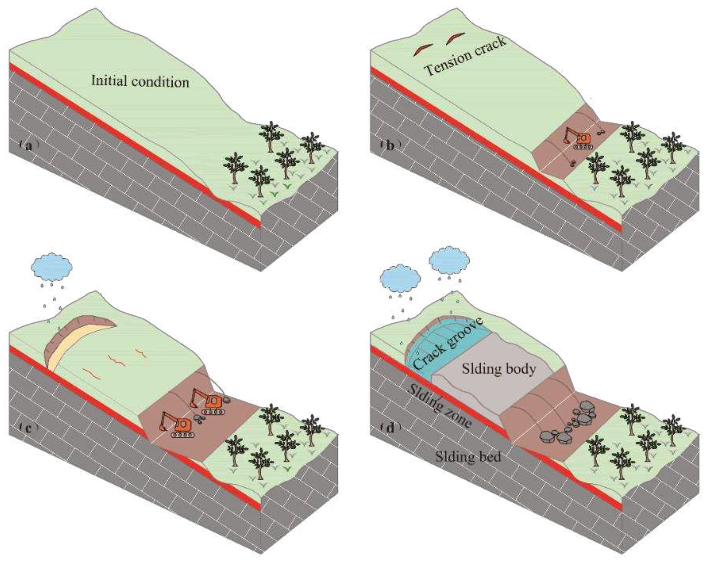
Figure 1. Evolution process of bedding rockslide under excavation unloading.
Preprints 95885 g001
Figure 2. Mechanical computational model for describing instability behavior: (a) combined (b) before instability, (c) moving, (d) the balance of slope in the end.
Preprints 95885 g002
Figure 3. Runout process of sliding body.
Preprints 95885 g003
Figure 4. Overview and basic characteristics of landslide.
Preprints 95885 g004
Figure 5. Engineering geological profile. a, b and c represent 1-1’, 2-2’ and 3-3’ respectively.
Preprints 95885 g005
Figure 6. Schematic slope geometry used in the numerical study.
Preprints 95885 g006
Figure 7. Slope deformation under the influence of excavation and hydrostatic pressure. (a, b) slope deformation under excavation conditions, (c, d) slope deformation combined excavation and hydrostatic pressure.
Preprints 95885 g007
Table 1. Calculation parameters of each section of Xinjianan landslide.
Profile γ (kN/m3) ɵ(°) β(°) h(m) b0 (m) h0 (m) L0 (m) W0 (kN/m) H (m)
1-1’ 21.5 82 74 19.4 1.5 5.5 196.0 62975.50 28.0
2-2’ 21.5 82 69 34.7 1.2 5.5 216.0 114972.54 42.6
3-3’ 21.5 82 76 19.1 2.2 3.5 30.0 9323.86 21.7
Table 2. Comparison between theoretical calculated and actual of landslide.
Profile lac (m) lac (m) Xt (m) Xt (m) absolute error relative error
1-1’ 170.5 187.2 75.22 69.5 16.7/5.72 8.9%/8.23%
2-2’ 175.2 197.7 82.5 72.4 22.5/1.83 11.38%/13.95%
3-3’ 20.8 25.7 27.14 25.7 4.0/0.15 19.07%/5.6%
Table 3. The materia properties of landslide.
Stage Position γ (kN/m3) B (Pa) S (Pa) c (kPa) φ (°) T(Mpa)
Excavation 1 21.5 7.2×10⁹ 5.5×10⁹ 26.3 24.4 1.5
2 19.5 3.8×10⁸ 2.1×10⁸ 19.5 21.5 0.35
3 25.5 8.9×10¹¹ 6.9×10¹¹ 95 50 120
Hydrostatic pressure 1 20.6 2.1×10⁹ 1.5×10⁹ 20.6 13.8 0.8
2 18.6 8.6×10⁷ 7.6×10⁷ 13.5 9.5 0.2
3 24.8 8.9×10¹¹ 6.9×10¹¹ 95 50 120
1~3 represent the sliding body, zone, and bed respectively. B: bulk modulus, S: shear modulus, T: tensile strength.
Table 4. Properties of rock matrix and joints.
Stage Position Jkn (GPa/m) Jks (GPa/m) Jc (kpa) Jt (Mpa) Jf (°)
Excavation 1 12.0 4.0 24.5 0.8 23.2
Hydrostatic pressure 1 10.0 2.5 19.8 0.4 12.5
Jkn/Jks: joint normal/shear stiffness; Jc: joint cohesion; Jt: joint tensile strength; Jf: joint friction.
Disclaimer/Publisher’s Note: The statements, opinions and data contained in all publications are solely those of the individual author(s) and contributor(s) and not of MDPI and/or the editor(s). MDPI and/or the editor(s) disclaim responsibility for any injury to people or property resulting from any ideas, methods, instructions or products referred to in the content.
Copyright: This open access article is published under a Creative Commons CC BY 4.0 license, which permit the free download, distribution, and reuse, provided that the author and preprint are cited in any reuse.
Prerpints.org logo

Preprints.org is a free preprint server supported by MDPI in Basel, Switzerland.

Subscribe

© 2024 MDPI (Basel, Switzerland) unless otherwise stated