This paper aims at achieving optimal rotor speed estimation for an induction motor using the Extended Kalman filter (EKF). Speed estimation is essential for fault diagnosis in Motor Current Signature Analysis (MCSA). The estimation accuracy is obtained by exploring the noise covariance matrices estimation of the EKF algorithm. The noise covariance matrices are determined using a modified subspace model identification approach. In order to reach this goal, this method compares an estimated model of a deterministic system, derived from available input-output datasets, with the discrete-time state-space representation used in the Kalman filter equations. This comparison leads to the determination of model uncertainties, which are subsequently represented as noise covariance matrices. Based on the 5th order nonlinear model of the induction motor, rotor speed is estimated with the optimized EKF algorithm and the used algorithm is tested experimentally.

Keywords:

Subject: Engineering - Control and Systems Engineering

1. Introduction

The induction motor (IM) is by far the most widely used motor in industry [1] as this motor is found in furnaces, conveyors, pumps and other industrial equipments. Monitoring and controlling induction motor speed is essential because changes or abnormalities in motor speed can indicate potential faults or malfunctions. Unfortunately, it can be challenging or exteremely expensive to use sensors for speed measurement of IM. In fact, some industrial environments may have unsuitable conditions for sensor implementation such as high temperatures, vibrations, or corrosive substances. To overcome these challenges, alternative methods can be employed for IM speed estimation. One commonly used technique consists in estimating the speed from the motor electrical variables only, such as stator currents and voltages. This is typically achieved using algorithms or observers such as Sliding Mode Observers [2], Model Reference Adaptive Systems [3] or the Extended Kal- man Filter [4,5,6,7,8,9]. Among all these methods, EKF method has attached significant attention due to its good estimation accuracy in the presence of noise. In the literature, there are different studies in which EKF based state/parameter estimation is executed. Those studies can be divided into two groups. The first group where EKF is applied, it is considered that no mechanical information is available [4,5,6]. The second group of solutions makes use of the rotational speed through the equations of motion [7,8,9]. The latter requires knowledge of the mechanical parameters such as load torque, inertia varying with the load coupled to the shaft, and viscous friction. In this paper, we focus on the first group of studies assuming the lack of information about the mechanical parameters.

One key feature of the Kalman filter is the requirement of the process and measurement noise covariance matrices. These matrices represent the noise levels in the system and have a direct impact on filter performance. In fact, incorrect or badly adjusted values of Q and R can lead to inaccurate estimation of the system state and filter instability. Furthermore, the parameters of the noise covariance matrices Q and R are usually determined by a trial-and-error procedures which may not give accurate results. As the distribution of noise is usually unknown, it is not possible to deduce a generic relationship between the values of the matrix elements and the EKF performance to yield the best speed estimation results.

The determination of noise covariance matrices is still open issues in practice. A significant part of the literature dedicated to Kalman filter tuning is devoted to the development of techniques and algorithms for the determination of these covariance matrices. However, there is a limited number of studies using covariance matrices estimation for induction motor speed estimation. In fact, researchers focus on investigating the optimization of noise covariance matrices for induction motor speed estimation. This investigation can be categorized into two main parts: the first group of studies [10,11] uses artificial intelligence-based methods which requires an expert knowledge and involves a complex design procedure, whereas the second group [12,13,14,15,16,17,18,19] employs adaptive structures to eliminate the adverse effect under operating condition variations.

The main contribution of this study is to design a fifth-order IM model, where the IM speed is included to the model as a state without the help of equation of motion and the noise covariance matrices are estimated. Among all of the Kalman filter tuning techniques available in the literature, a specific attention is paid herein to the noise covariance matrices estimation with modified subspace model identification method [20]. The method consists in translating the discrepancy between the identified model (determined from the available input−output datasets) and the discrete-time state space representation involved in the Kalman filter equations into noise covariance matrices estimates. The model identification method used in [20] was derived from the subspace model identification methods [21,22,23,24] and adapted to estimate a discrete linear time invariant state space model. The main motivation for selecting this class of methods is the strong and inherent link between the subspace identification methods and Kalman filtering [25].

In this paper, a noise covariance matrices estimation with a modified subspace model identification method is employed in order to achieve the best EKF performance in the speed motor estimation. In order to reach this goal, the paper is organized as follows: Section 1 presents the dynamic model of the induction motor and the extended dynamic model of the IM to be used in the EKF. Section 2 details the design of the EKF to estimate the motor speed. Section 3 presents the noise covariance matrices estimation procedure by using a modified subspace model identification method. Section 4 is devoted to the application of the modified subspace model identification method to rotor speed estimation. Section 5 compares the experimental performance of the trial-and-error-process method and the modified subspace model identification method used to determine the noise covariance matrices of the EKF in the case of rotor speed estimation. Finally, Section 6 gives the conclusion.

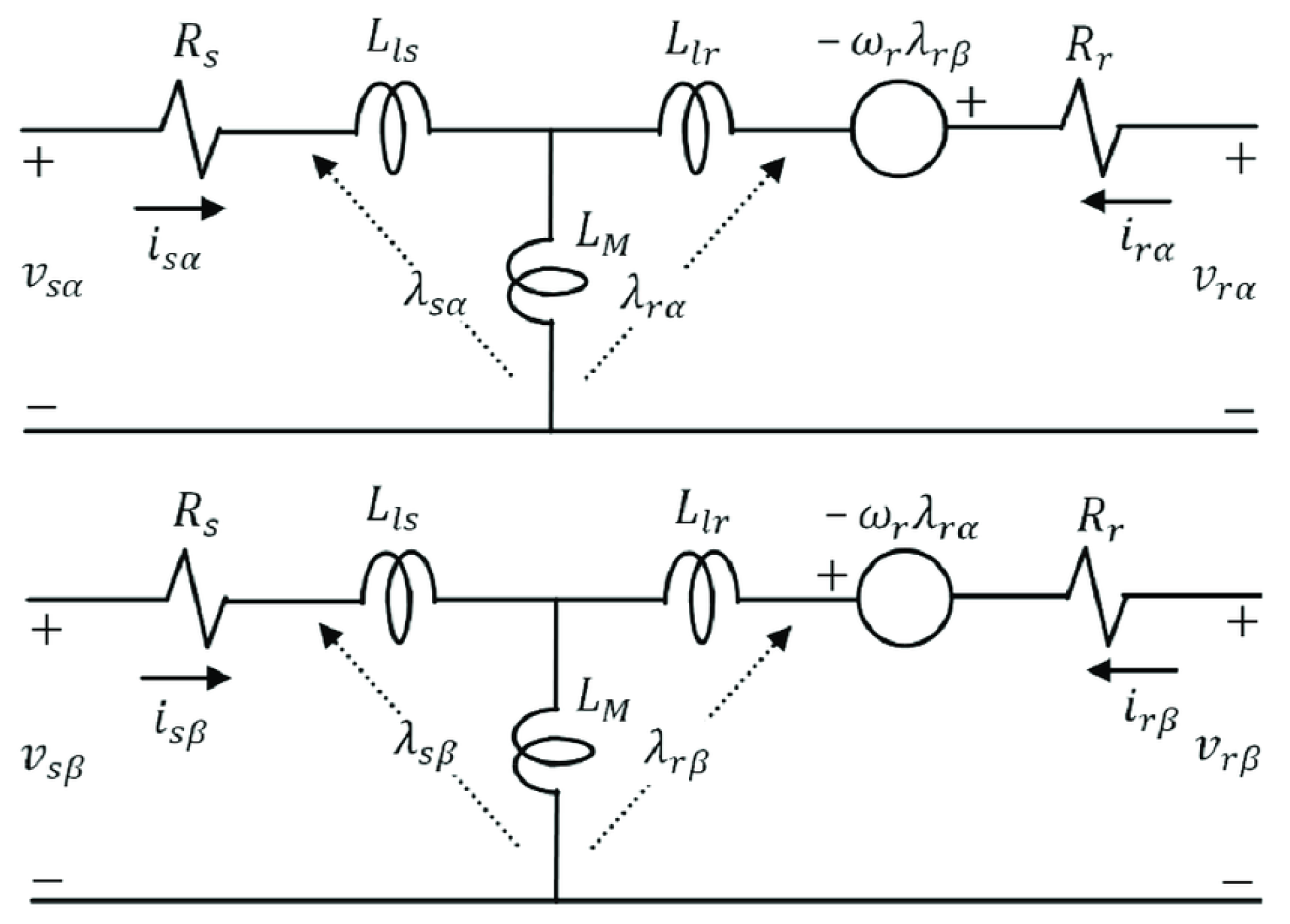
2. Dynamic model of induction motor

In order to estimate the rotor speed of IM using EKF, the mathematical model of the three-phase induction motor is developped. Because three-phase systems involve complex quantities and calculations, the analysis of the three-phase induction motor is simplified using the Clarke transformation. In this way, the three-phase quantities (a, b, c) are transformed into two-phase quantities (

α

β

) which are aligned with the stator (stationnary reference frame) [26].

Figure 1 shows the equivalent circuit of the IM in the stationnary reference frame [27].

In this equivalent circuit,

R_{s}

L_{1 s}

are the stator resistance and inductance, respectively;

R_{r}

and

L_{1 r}

are the rotor resistance and inductance referred to the stator side, respectively;

L_{m}

is the mutual inductance;

ω_{r}

is the rotor speed;

v_{s α}

v_{s β}

are the measured stator voltages and

i_{s α}

i_{s β}

are the stator currents in the stationary reference frame;

v_{r α}

v_{r β}

are the rotor voltages and and

i_{r α}

i_{r β}

are the rotor currents in the stationary reference frame;

λ_{s α} (t)

λ_{s β} (t)

are the stator flux and and

λ_{r α} (t)

λ_{r β} (t)

are the rotor flux in the stationary reference frame.

Figure 1 helps to understand the electrical and magnetic energy exchanges present in the induction motor and allows to derive the mathematical equations.

First, let us introduce a state-space representation of IM dynamics, assuming that IM speed is a known parameter

\dot{x} (t) = A x (t) + B u (t),

(1a)

y (t) = C x (t),

(1b)

where

x (t)

stands for the state vector,

y (t)

is the output vector and

u (t)

is the input vector, with

$x (t) = {[i_{s α} (t) i_{s β} (t) λ_{r α} (t) λ_{r β} (t)]}^{T}$ ,
$y (t) = {[i_{s α} (t) i_{s β} (t)]}^{T}$ ,
$u (t) = {[v_{s α} (t) v_{s β} (t)]}^{T}$ ,
$A = [\begin{matrix} - \frac{K_{r}}{K_{l}} & 0 & \frac{L_{m} R_{r}}{L_{r}^{2} K_{l}} & \frac{p L_{m} ω_{r}}{2 L_{r} K_{l}} \\ 0 & - \frac{K_{r}}{K_{l}} & - \frac{p L_{m} ω_{r}}{2 L_{r} K_{l}} & \frac{L_{m} R_{r}}{L_{r}^{2} K_{l}} \\ \frac{L_{m}}{τ_{r}} & 0 & - \frac{1}{τ r} & - \frac{p}{2} ω_{r} \\ 0 & \frac{L_{m}}{τ_{r}} & \frac{p}{2} ω_{r} & - \frac{p}{2} ω_{r} \end{matrix}],$
$B = [\begin{matrix} \frac{1}{K_{l}} & 0 \\ 0 & \frac{1}{K_{l}} \\ 0 & 0 \\ 0 & 0 \end{matrix}]$ ,
$C = [\begin{matrix} 1 & 0 & 0 & 0 \\ 0 & 1 & 0 & 0 \end{matrix}]$ ,

where p is number of poles,

τ_{r} = L_{r} / R_{r}

is the rotor time constant,

K_{r} = R_{r} + {L_{m}}^{2} R_{r} / {L_{r}}^{2}

and

K_{l} = (1 - {L_{m}}^{2} / L_{r} / L_{s}) L_{s}

with

L_{s} = L_{1} s + L_{m}

and

L_{r} = L_{1} r + L_{m}

As mentionned above, the rotor speed

ω_{r}

in equations (1a) and (1b) is considered as a known parameter. If the speed measurement is not available, the rotor speed has to be estimated. To this end, an extended induction motor model including the rotor speed as state variable is developped [4,5]. The rotor speed is then considered both as a state and a parameter, leading to a nonlinear IM model defined as

\dot{x_{e}} (t) = f_{e} (x_{e} (t), u (t)),

(2a)

y (t) = C_{e} x_{e} (t),

(2b)

where

f_{e}

is the nonlinear function of the states and inputs defined as

f_{e} (x_{e} (t), u (t)) = A_{e} x_{e} (t) + B_{e} u (t),

(3)

with

$x_{e} (t) = {[i_{s α} (t) i_{s β} (t) λ_{r α} (t) λ_{r β} (t) ω_{r} (t)]}^{T}$ ,
$u (t) = {[v_{s α} (t) v_{s β} (t)]}^{T}$ ,
$A_{e} = [\begin{matrix} - \frac{K_{r}}{K_{l}} & 0 & \frac{L_{m} R_{r}}{L_{r}^{2} K_{l}} & \frac{p L_{m} ω_{r} (t)}{2 L_{r} K_{l}} & 0 \\ 0 & - \frac{K_{r}}{K_{l}} & - \frac{p L_{m} ω_{r} (t)}{2 L_{r} K_{l}} & \frac{L_{m} R_{r}}{L_{r}^{2} K_{l}} & 0 \\ \frac{L_{m}}{τ_{r}} & 0 & - \frac{1}{τ r} & - \frac{p}{2} ω_{r} (t) & 0 \\ 0 & \frac{L_{m}}{τ_{r}} & \frac{p}{2} ω_{r} (t) & - \frac{1}{τ r} & 0 \\ 0 & 0 & 0 & 0 & 0 \end{matrix}],$
$B_{e} = [\begin{matrix} \frac{1}{K_{l}} & 0 \\ 0 & \frac{1}{K_{l}} \\ 0 & 0 \\ 0 & 0 \\ 0 & 0 \end{matrix}]$ ,
and
$y (t) = {[i_{s α} (t) i_{s β} (t)]}^{T}$ ,
$C_{e} = [\begin{matrix} 1 & 0 & 0 & 0 & 0 \\ 0 & 1 & 0 & 0 & 0 \end{matrix}]$ .
Because this extended IM model is non linear, the EKF algorithm is used in order to estimate the rotor speed.

3. EKF algorithm for rotor speed estimation

To estimate rotor speed in real-time with the EKF, the continuous-time state equations developed previously in (2a) and (2b) are discretized with a sampling period

T_{s}

using the Euler approximation method [28] as follows

{\hat{x}}_{k + 1} = F {\hat{x}}_{k} + G u_{k},

(4a)

{\hat{y}}_{k} = H {\hat{x}}_{k},

(4b)

where

{\hat{x}}_{k} = {[i_{s α, k} i_{s β, k} λ_{r α, k} λ_{r β, k} ω_{r, k}]}^{T}

y_{k} = {[i_{s α, k} i_{s β, k}]}^{T}

u_{k} = {[v_{s α, k} v_{s β, k}]}^{T}

and

F = I + A_{e} T_{s},

(5a)

G = T_{s} B_{e},

(5b)

H = C_{e},

(5c)

with

F = [\begin{matrix} 1 - \frac{K_{r}}{K_{l}} T_{s} & 0 & \frac{L_{m} R_{r}}{L_{r}^{2} K_{l}} T_{s} & \frac{p L_{m} ω_{r, k}}{2 L_{r} K_{l}} T_{s} & 0 \\ 0 & 1 - \frac{K_{r}}{K_{l}} T_{s} & - \frac{p L_{m} ω_{r, k}}{2 L_{r} K_{l}} T_{s} & \frac{L_{m} R_{r}}{L_{r}^{2} K_{l}} T_{s} & 0 \\ \frac{L_{m}}{τ_{r}} T s & 0 & 1 - \frac{1}{τ_{r}} T_{s} & - \frac{p}{2} ω_{r, k} T_{s} & 0 \\ 0 & \frac{L_{m}}{τ_{r}} T s & \frac{p}{2} ω_{r, k} T_{s} & 1 - \frac{1}{τ_{r}} T_{s} & 0 \\ 0 & 0 & 0 & 0 & 1 \end{matrix}]

G = [\begin{matrix} \frac{T_{s}}{K_{l}} & 0 \\ 0 & \frac{T_{s}}{K_{l}} \\ 0 & 0 \\ 0 & 0 \\ 0 & 0 \end{matrix}]

H = [\begin{matrix} 1 & 0 & 0 & 0 & 0 \\ 0 & 1 & 0 & 0 & 0 \end{matrix}]

In order to take into account the uncertainties and discrepancies between the mathematical model and the real system being observed, the process noise

w_{k}

and measurement noise

v_{k}

are introduced into the state-space representation as

{\hat{x}}_{k + 1} = F {\hat{x}}_{k} + G u_{k} + w_{k},

(6a)

y_{k} = H {\hat{x}}_{k} + v_{k},

(6b)

The covariance matrices of the process noise

w_{k}

and measurement noise

v_{k}

can be defined as

E [[\begin{matrix} v_{i} \\ w_{i} \end{matrix}] [\begin{matrix} v_{j}^{T} & w_{j}^{T} \end{matrix}]] = [\begin{matrix} R & S \\ S^{T} & Q \end{matrix}] δ_{i j},

(7)

where

δ_{i j}

is the Kronecker delta function.

Using conventional equations of the EKF algorithm [29], induction motor speed is estimated as follows

{\hat{x}}_{k + 1}^{-} = F {\hat{x}}_{k}^{+} + G u_{k},

(8a)

P_{k + 1}^{-} = J_{k + 1} P_{k}^{+} J_{k + 1}^{T} + Q_{k},

(8b)

K_{k} = P_{k}^{-} H_{k}^{T} {(H_{k} P_{k}^{-} H_{k}^{T} + R_{k})}^{- 1},

(8c)

{\hat{x}}_{k + 1}^{+} = {\hat{x}}_{k + 1}^{-} + K_{k + 1} (y_{k + 1} - {\hat{y}}_{k + 1}),

(8d)

P_{k + 1}^{+} = (I - K_{k + 1} H_{k + 1}) P_{k + 1}^{-},

(9)

where the notations ⁻ and ⁺ stand for before and after new measurements,

P_{k}

is the error covariance matrix,

K_{k}

is the Kalman filter gain,

{\hat{y}}_{k}

is the estimated output and

J_{k}

is the Jacobian matrix used in the EKF to handle nonlinearities, defined as

J_{k} = \frac{\partial F}{\partial x} |_{x = {\hat{x}}_{k}^{+}},

(10)

with

J_{k} = [\begin{matrix} 1 - \frac{K_{r}}{K_{l}} T_{s} & 0 & \frac{L_{m} R_{r}}{L_{r}^{2} K_{l}} T_{s} & \frac{p L_{m} ω_{r}}{2 L_{r} K_{l}} T_{s} & \frac{p L_{m}}{2 L_{r} K_{l}} T_{s} λ_{β r} \\ 0 & 1 - \frac{K_{r}}{K_{l}} T_{s} & - \frac{p L_{m} ω_{r}}{2 L_{r} K_{l}} T_{s} & \frac{L_{m} R_{r}}{L_{r}^{2} K_{l}} T_{s} & - \frac{p L_{m}}{2 L_{r} K_{l}} T_{s} λ_{α r} \\ \frac{L_{m}}{τ_{r}} T_{s} & 0 & 1 - \frac{1}{τ_{r}} T_{s} & - \frac{p}{2} ω_{r} T_{s} & - \frac{p}{2} T_{s} λ_{β r} \\ 0 & \frac{L_{m}}{τ_{r}} T_{s} & \frac{p}{2} ω_{r} T_{s} & 1 - \frac{1}{τ_{r}} T_{s} & - \frac{p}{2} T_{s} λ_{α r} \\ 0 & 0 & 0 & 0 & 1 \end{matrix}] .

4. Noise covariance matrices estimation with a modified subspace model identification approach

As mentioned earlier, using the Kalman filter requires defining the process and measurements covariance matrices. These matrices are essential for quantifying the noise levels and model uncertainties. Gererally, the parameters of the noise covariance matrices Q and R are determined by a trial-and-error-process that can be challenging. In fact, improper or poorly calibrated values of Q and R can lead to inaccurate estimations of the system states.

In order to relieve this inconvenience, the noise covariance matrices can be estimated. Among all of the tuning techniques available in the literature, a specific attention is paid herein to the noise covariance matrices estimation with a modified subspace model identification approach [20].

The solution proposed in this approach consists in:

identifying a state-space matrices $A_{d}$ , $B_{d}$ , $C_{d}$ , $D_{d}$ and state sequence ${\hat{X}}_{f, N}$ with $f, N \in N_{*}^{+}$ from available input-output data using subspace model identification method. The identified state sequence ${\hat{X}}_{f, N}$ can be defined as

${\hat{X}}_{f, N} = [\begin{matrix} {\hat{X}}_{f} \\ {\hat{X}}_{f + 1} \\ ⋮ \\ {\hat{X}}_{f + N - 1} \end{matrix}] \in R^{n_{x} \times N},$

(11)

with ${\hat{X}}_{f, N} \in R^{n_{x}}$ ;
comparing the identified state-space model with the deterministic part of the model used in the Kalman Filter. To this end, the both models have to be in the same basis. Therefore, we proceed to a basis change using transformation matrix T which can be computed as

$Γ_{f} (F, H) T = {\hat{Γ}}_{f} (A_{d}, C_{d}),$

(12)

where $Γ_{f} (F, H)$ is the observability matrix of the model used in the Kalman Filter defined as

$Γ_{l} (F, H) = {[H^{T} {(H F)}^{T} \dots {(H F^{l - 1})}^{T}]}^{T},$

(13)

and ${\hat{Γ}}_{f} (A_{d}, C_{d})$ is the observability matrix of the identified model using subspace model identification method defined as

${\hat{Γ}}_{l} (A_{d}, C_{d}) = {[C_{d}^{T} {(C_{d} A_{d})}^{T} \dots {(C_{d} A_{d}^{l - 1})}^{T}]}^{T} .$

(14)

Once $\hat{T}$ is estimated with a Moore Penrose pseudo inverse, the state sequence ${\hat{X}}_{f, N}$ can be moved into the "good" state basis as follows

${\hat{\hat{X}}}_{f, N} = \hat{T} {\hat{X}}_{f, N} .$

(15)
computing the residuals as

$[\begin{matrix} {\hat{Q}}_{f, 1, N - 1} \\ {\hat{R}}_{f, 1, N - 1} \end{matrix}] = [\begin{matrix} {\hat{\hat{X}}}_{f + 1, N} \\ Y_{f, 1, N - 1} \end{matrix}] - [\begin{matrix} F & G \\ H & 0 \end{matrix}] [\begin{matrix} {\hat{\hat{X}}}_{f, N - 1} \\ U_{f, 1, N - 1} \end{matrix}],$

(16)

where $\hat{\hat{X}}$ with $f, N \in N_{*}^{+}$ represents the state sequence estimate in the "good" state basis performed with subspace model identification method, and ${\hat{Q}}_{f, 1, N - 1}$ , ${\hat{R}}_{f, 1, N - 1}$ are residuals used to estimate the covariance matrices Q and R.
transforming this discrepancy measurements into covariance matrix estimates. This part will be detailed next.

4.1. Subspace model identification

Before describing the the subspace model identification method, let us introduce the following notation. For any vector

r_{k} \in R^{n_{r}}

and parameters f,l and

N \in N_{*}^{+}

, the block Hankel matrix is defined as follows

R_{f, l, N} = [\begin{matrix} r_{f} & r_{f + 1} & \dots & r_{f + N - 1} \\ r_{f + 1} & r_{f + 2} & \dots & r_{f + N} \\ ⋮ & ⋱ & ⋱ & ⋮ \\ r_{f + l - 1} & r_{f + l} & \dots & r_{f + N + l - 2} \end{matrix}] \in R^{l n_{r} \times N} .

(17)

According to [30], consider the minimal system

x_{k + 1} = A_{d} x_{k} + B_{d} u_{k} + K e_{k},

(18a)

y_{k} = C_{d} x_{k} + D_{d} u_{k} + e_{k},

(18b)

with

e_{k}

a white-noise sequence that is uncorrelated with

u_{k}

By taking the instrumental-variable matrix

Z_{N}

equal to

Z_{N} = [\begin{matrix} U_{0, l, N} \\ Y_{0, l, N} \end{matrix}],

(19)

where

U_{0, l, N}

and

Y_{0, l, N}

with

l, N \in N_{*}^{+}

are the block Hankel matrices constructed from input-output data, and by considering the following least-squares problem

[\begin{matrix} {\hat{L}}_{N}^{u} & {\hat{L}}_{N}^{z} \end{matrix}] = arg min_{L^{u}, L z} | | Y_{l, l, N} - [\begin{matrix} L^{u} & L^{z} \end{matrix}] [\begin{matrix} U_{l, l, N} \\ Z_{N} \end{matrix}] | |_{F}^{2},

(20)

which is solved by a QR factorisation

[\begin{matrix} U_{f, l, N} \\ U_{0, l, N} \\ Y_{0, l, N} \\ Y_{f, l, N} \end{matrix}] = [\begin{matrix} R_{11} & 0 & 0 \\ R_{21} & R_{22} & 0 \\ R_{31} & R_{32} & R_{33} \end{matrix}] [\begin{matrix} Q_{1} \\ Q_{2} \\ Q_{3} \end{matrix}],

(21)

it can be shown [30] that

(lim_{N \to \infty} {\hat{L}}_{N}^{Z}) Z_{N} = (lim_{N \to \infty} R_{32} R_{22}^{- 1}) Z_{N},

(22)

and

R_{32} R_{22}^{- 1} [\begin{matrix} U_{0, l, N} \\ Y_{0, l, N} \end{matrix}] = Γ_{f} (A_{d}, C_{d}) {\hat{X}}_{f, N} .

(23)

Via the following singular value decomposition

R_{32} R_{22}^{- 1} [\begin{matrix} U_{0, l, N} \\ Y_{0, l, N} \end{matrix}] = {υ Σ ν}^{T},

(24)

we get an estimate of the observability matrix as follows

{\hat{Γ}}_{f} (A_{d}, C_{d}) = υ Σ^{1 / 2},

(25)

whereas

{\hat{X}}_{f, N} = Σ^{1 / 2} ν^{T} .

(26)

As mentionned earlier, the state sequence

{\hat{X}}_{f, N}

has to be in the "good" state basis corresponding to the state-space realization used in the Kalman filter (F, G, H). Thus, we proceed to a basis change using equation (12).

Knowing the estimated state sequence

{\hat{\hat{X}}}_{f, N}

, we can quantify the discrepancy between this prior information and the model used in the Kalman Filter using equation (16).

4.2. Noise covariance matrices estimation

We can determine now an accurate estimates of the covariance matrices Q, and R using the residuals computed in equation (16), as follows [21]

[\begin{matrix} \hat{R} & \hat{S} \\ {\hat{S}}^{T} & \hat{Q} \end{matrix}] = lim_{N \to \infty} \frac{1}{N} [\begin{matrix} {\hat{Q}}_{f, 1, N - 1} \\ {\hat{R}}_{f, 1, N - 1} \end{matrix}] [\begin{matrix} {\hat{Q}}_{f, 1, N - 1}^{T} & {\hat{R}}_{f, 1, N - 1}^{T} \end{matrix}] .

(27)

5. Induction Motor Speed Estimation with noise covariance matrices estimation

As discussed earlier, the speed induction motor estimation using EKF requires a dynamic state space model presented in equations (2a) and (2b). This dynamic model which includes the rotor speed as state space is non observable. Or, the noise covariance matrices estimation with the modified subspace model identification approach presented previously requires an observable model.

As a solution, we propose to identify only the dynamic model which does not include the rotor speed as state variable as described by equations (1a) and (1b). This 4^th order model leads to determine the covariance matrices

Q_{1}

and

R_{1}

of the system noise and measurement noise respectively.

In order to determine the covariance matrices of the dynamic model which is able to estimate the rotor speed, the measurement noise covariance matrix R is the same as the 4^th order model beacause it depends only of the measurements. Unlike to the system noise covariance matrix which depends of the estimated states.

Thus, in the new system noise covariance matrix, we have to only adjust the parameter

μ

as shown below

Q = [\begin{matrix} q_{11} & q_{12} & q_{13} & q_{14} & 0 \\ q_{21} & q_{22} & q_{23} & q_{24} & 0 \\ q_{31} & q_{32} & q_{33} & q_{34} & 0 \\ q_{41} & q_{42} & q_{43} & q_{44} & 0 \\ 0 & 0 & 0 & 0 & μ \end{matrix}]

(28)

where the parameters

q_{n y}

with n number of row and y number of column are determined with a modified subspace model identification approach.

6. Results and discussion

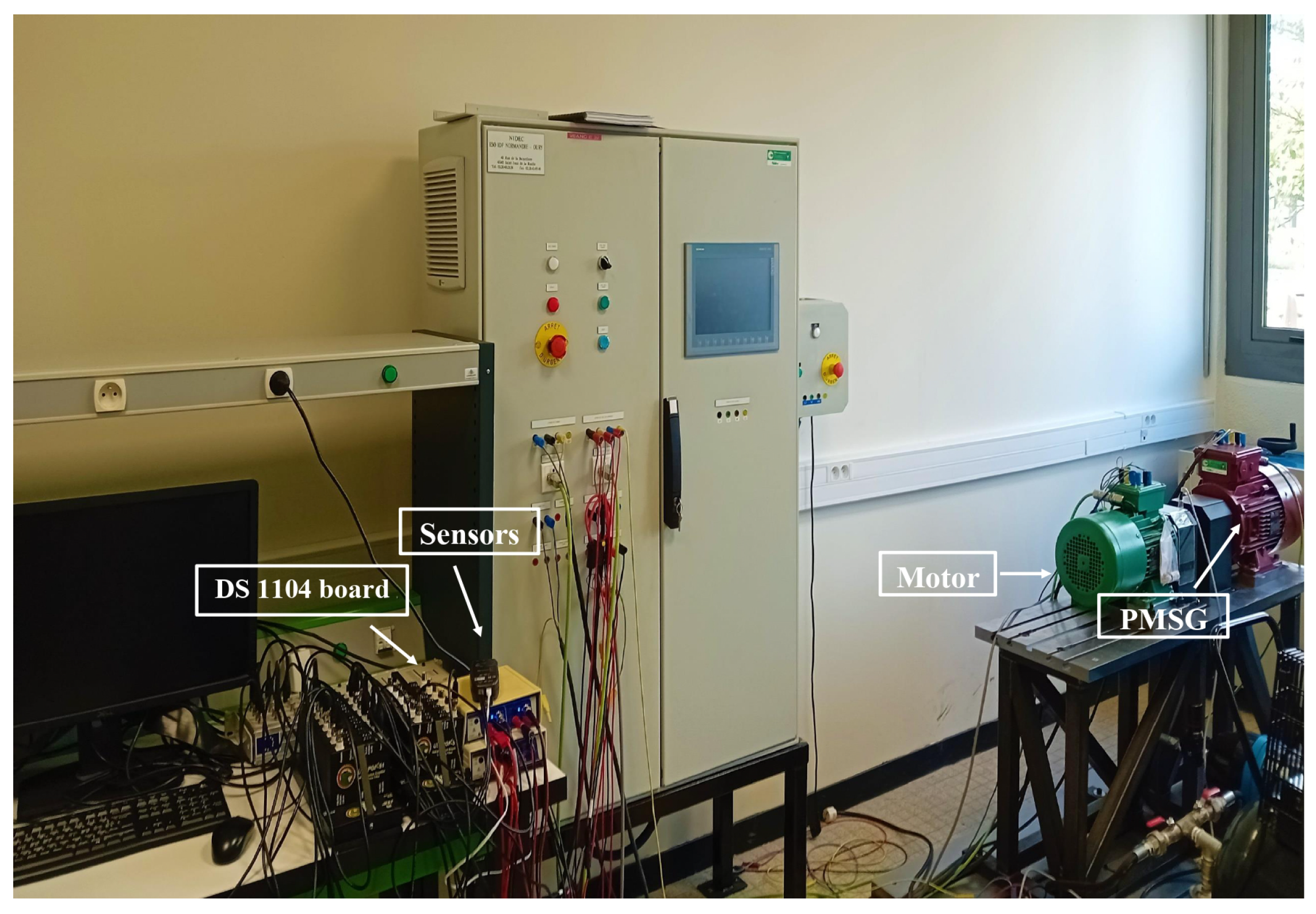
To justify the need of automated tuning of EKF, the speed estimation algorithm of the extended Kalman filter tunned by a trial-and-error-process is tested on our test bench presented below.

6.1. Experimental setup

The experimental test setup consists of a squirrel-cage induction motor

4 k W

220 V

50 H z

, 2poles controlled by an AC drive and coupled to a permanent magnet synchronous generator (PMSG) operating as a generator which produce a resisting torque thus representing the load.

The induction motor has the following parameters

R_{s} = 1.47 Ω

;

R_{r} = 0.78 Ω

;

L_{1 s} = 5.16 Ω

;

L_{1 r} = 0

;

R_{m} = 917.71 Ω

;

L_{m} = 90.139 Ω

In order to confirm the accurate estimation of the rotor speed with EKF algorithm, an encoder is employed to measure the real motor speed. The phase voltages and currents that represent the inputs and the outputs of the system respectively are also measured with sensors. A DS1104 board, which is compatible with MATLAB/Simulink software, is used to obtain measurements and apply the EKF speed estimation algorithm. The sampling period is

T s = 10^{- 3}

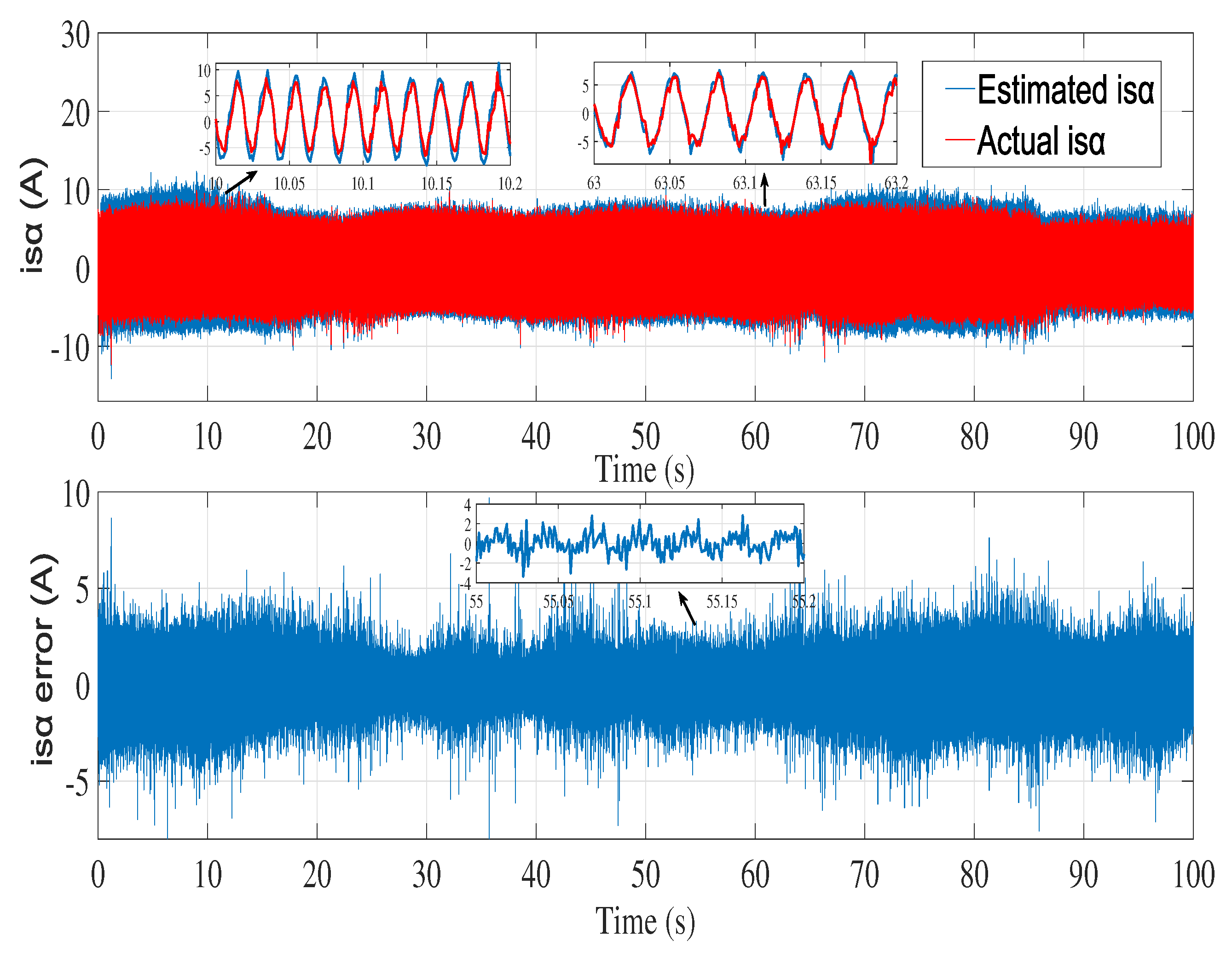
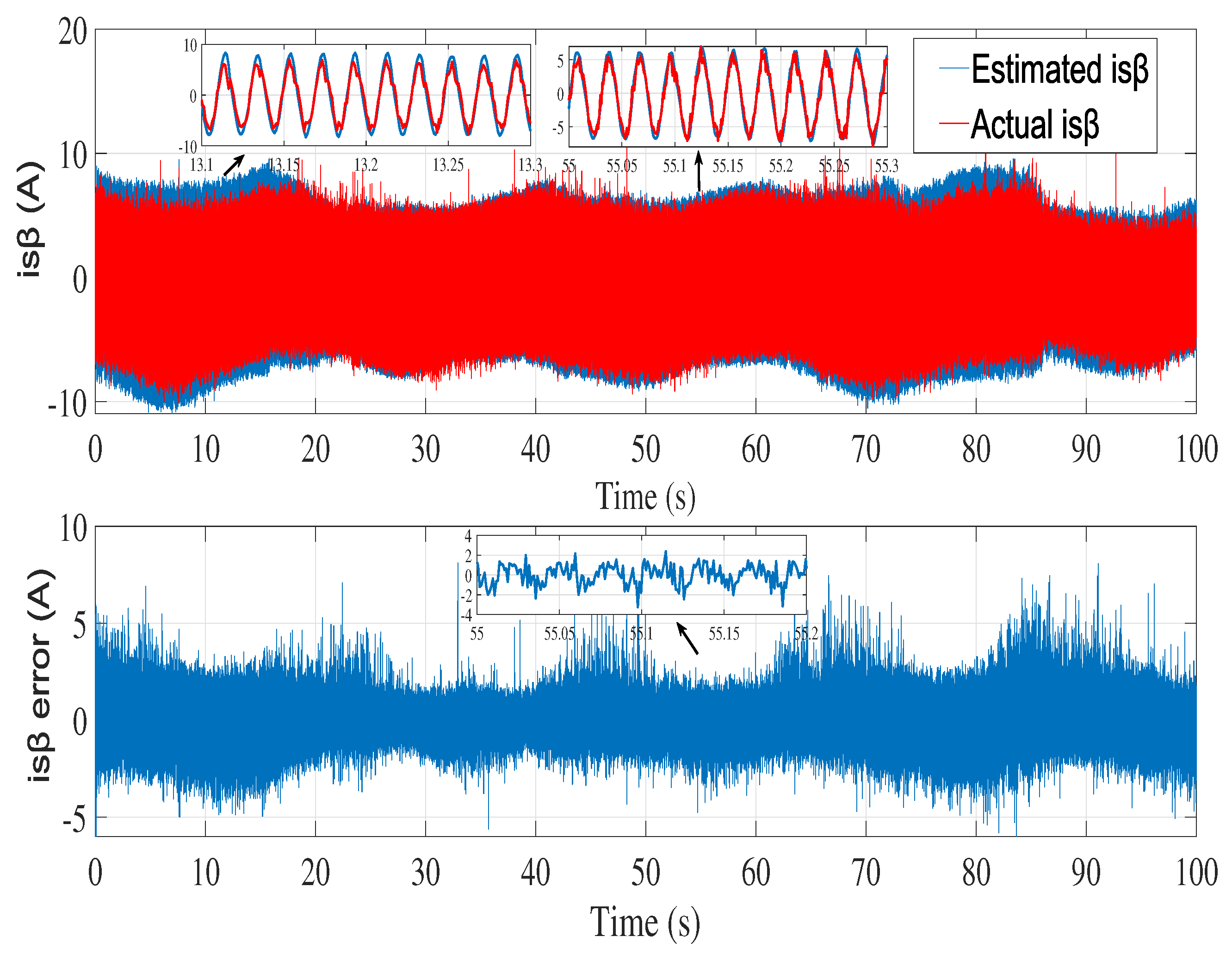
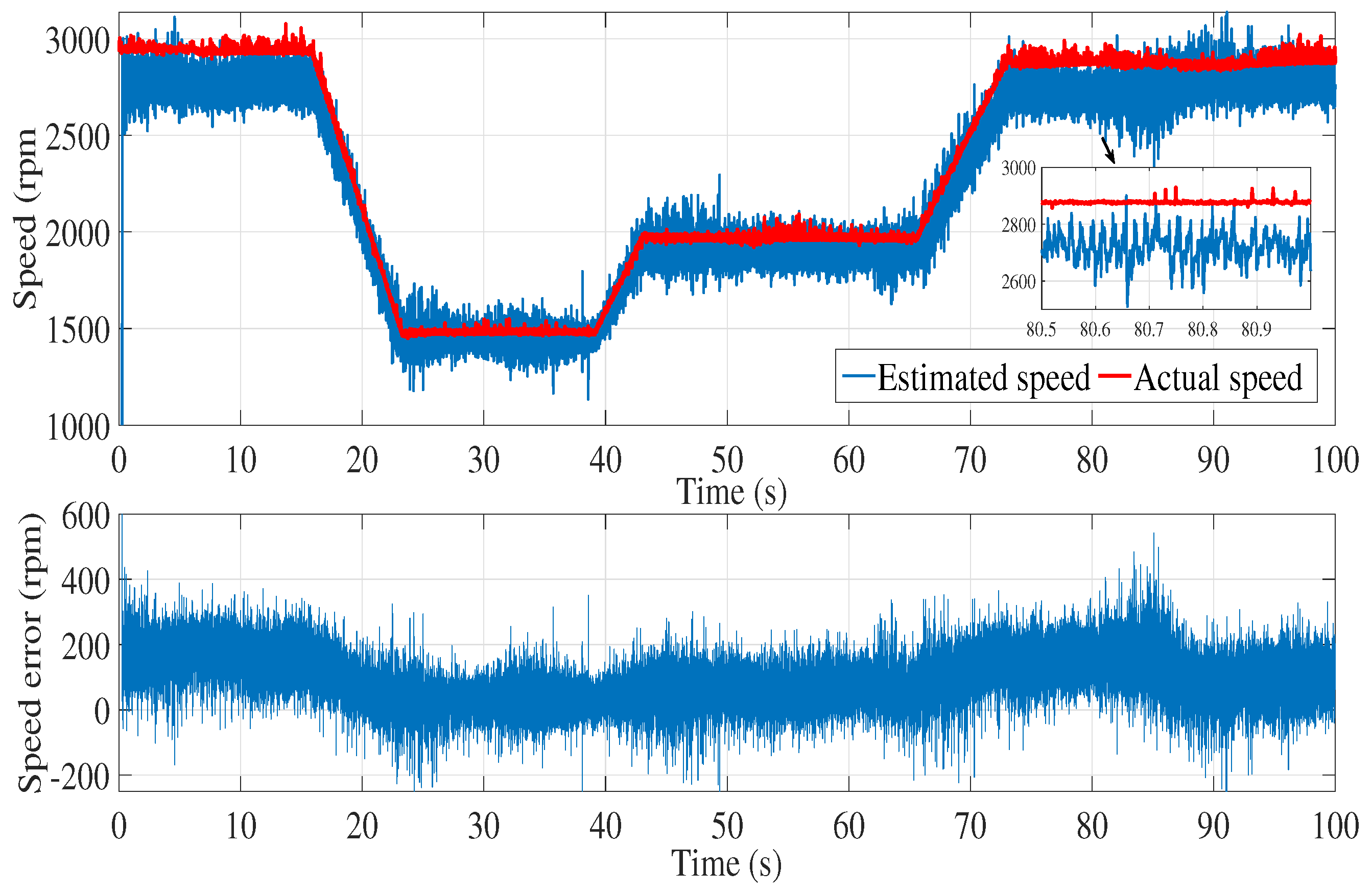
6.2. Experimental results

The covariance matrices used in the EKF algorithm and tuned by a trial-and-error method until satisfactory estimation performance is obtained are

Q = [\begin{matrix} λ & 0 & 0 & 0 & 0 \\ 0 & λ & 0 & 0 & 0 \\ 0 & 0 & λ & 0 & 0 \\ 0 & 0 & 0 & λ & 0 \\ 0 & 0 & 0 & 0 & μ \end{matrix}],

with

λ = 2

and

μ = 20

R = [\begin{matrix} 10^{- 3} & 0 \\ 0 & 10^{- 3} \end{matrix}],

and the error covariance matrix is initiallized as

P = [\begin{matrix} 1 & 0 & 0 & 0 & 0 \\ 0 & 1 & 0 & 0 & 0 \\ 0 & 0 & 1 & 0 & 0 \\ 0 & 0 & 0 & 1 & 0 \\ 0 & 0 & 0 & 0 & 1 \end{matrix}],

Figure 3 and Figure 4 show the estimated currents

i s_{α}

and

i s_{β}

, respectively, using trial-and-error method

whereas Figure 5 shows the estimated speed of the EKF using trial-and-error method

As we can see in the above figure, the estimated speed is very noisy. This can be justified by the

μ

coefficient, which is very large.

In order to minimize the effect of the noise in the estimated speed, the coefficient

μ

has to be reduced. However, smaller value of

μ

leads to innacurate estimation of the motor speed. In fact, the process noise covariance matrix Q, represents the uncertainty in the system dynamics and reflects the model accuracy in predicting the state evolution of the system. The values of the elements in the process noise covariance matrix determine how much the filter trusts the predicted state versus the measured state. Higher values indicate higher uncertainty in the system, leading to more reliance on the measurements. Furthermore, the error between the estimated and measured speed is more significant in the time interval of

80 \leq t \geq 85 s

A second attempt is now made to estimate the speed with the same noise covariance matrices of the first test

Figure 7.

i s_{β}

estimation using EKF tunned by a trial-and-error method-Second test.

Figure 7.

i s_{β}

estimation using EKF tunned by a trial-and-error method-Second test.

As it is shown in the Figure 8, the speed estimation using the same covariance matrices is innacurate in the time interval of

50 \leq t \geq 70 s

. Therefore, the noise matrices must be modified each time.

Consequently, manual tuning of the EKF using trial-and-error-process is proven to be inefficient. It is time-consuming and requires significant effort from an experienced operator. Moreover, it involves the configuration of multiple parameters of the noise covariance matrices.

To overcome this difficulty, the noise covariance matrices are determined with a subspace model identification approach.

Because the model used to estimate the rotor speed is nonlinear and the subspace model identification method requires linear time invariant state space representation, the nonlinear model is linearized around the known nominal rotor speed.

In addition, system identification requires exciting the inputs and outputs of the system (voltages and currents respectively). To this end and from the same test bench, a pseudo random binary sequence (PRBS) is applied as a desired speed (Figure 9) and is varying around the nominal speed (2920 rpm)

Excited voltages and currents are then used to identify a discrete time linear state space of the system.

Figure 10 gives the block diagram of experimental setup used to estimate the noise covariance matrices

The identification efficiency is evaluated by comparing the identified and actual currents (system outputs) as shown in Figure 11 and Figure 12

The best fits obtained by comparing the identified and actual currents are

78.73 %

for

i_{s α}

and

79.73 %

for

i_{s β}

In fact, mathematical models are often simplified approximations of reality and may not always capture all the details of the system’s behavior or take into account the nonlinearities.

The noise covariance matrices are now determined using the modified subspace model identification

Q_{1} = [\begin{matrix} 2.46 & 0.08 & - 1.96 & - 3.88 \\ 0.08 & 0.81 & 2.420 & - 1.58 \\ - 1.96 & 2.42 & 9.97 & - 0.87 \\ - 3.88 & - 1.58 & - 0.87 & 10.14 \end{matrix}]

R = [\begin{matrix} 2.51 & - 3.90 \\ - 3.90 & 12.21 \end{matrix}]

We can now reconstruct the process noise covariance matrix as

Q = [\begin{matrix} 2.46 & 0.08 & - 1.96 & - 3.88 & 0 \\ 0.08 & 0.81 & 2.420 & - 1.58 & 0 \\ - 1.96 & 2.42 & 9.97 & - 0.87 & 0 \\ - 3.88 & - 1.58 & - 0.87 & 10.14 & 0 \\ 0 & 0 & 0 & 0 & μ \end{matrix}]

Using this identified process noise covariance matrix Q and measurement noise covariance matrix R to estimate the rotor speed of the same test bench described before and by varying the

μ

coefficient until a satisfactory result, the resulting estimations are presented in the below Figures

Figure 13.

i s_{α}

estimation with EKF using noise covariance matrices estimation-First test.

Figure 13.

i s_{α}

estimation with EKF using noise covariance matrices estimation-First test.

Figure 14.

i s_{β}

estimation with EKF using noise covariance matrices estimation-First test.

Figure 14.

i s_{β}

estimation with EKF using noise covariance matrices estimation-First test.

Figure 15. IM speed estimation with EKF using noise covariance matrices estimation-First test.

The accurate speed estimation is obtained for

μ = 40

The speed estimation error has decreased comparing to the trial-and-error process tuning.

Figure 16.

i s_{α}

estimation with EKF using noise covariance matrices estimation-Second test.

Figure 16.

i s_{α}

estimation with EKF using noise covariance matrices estimation-Second test.

Figure 17.

i s_{β}

estimation with EKF using noise covariance matrices estimation-First test.

Figure 17.

i s_{β}

estimation with EKF using noise covariance matrices estimation-First test.

Figure 18. IM speed estimation with EKF using noise covariance matrices estimation-Second test.

We apply now the same noise covariance matrices to the second test

As we can see, the identified noise covariance matrices are valid for both tests, unlike the trial-and-error-process method where the noise covariance matrices have to be set each time.

Furthermore, Figure 19 shows a comparison between measured speed, estimated speed using manual tuning and estimated speed using modified subspace identification approach of the first test

As it’s shown, the effect of noise has been minimized using automated tuning of the covariance matrices.

Finally, the table below provides a comparison between the mean squared error of the estimated speed for both the trial-and-error process method and automated tuning of the EKF

The mean squared error between the actual rotor speed and the estimated speed is defined as

E = \frac{1}{n} \sum_{i = 1}^{n} {(s_{i} - e_{i})}^{2}

(29)

with n is the number of samples, s is the actual speed and e is the estimated speed.

It is observed that the estimation has significantly improved for both first and second test.

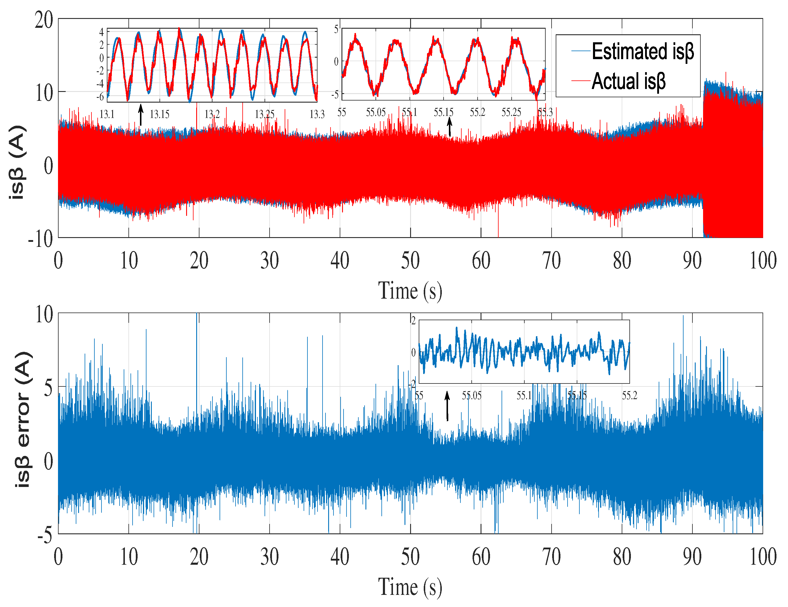
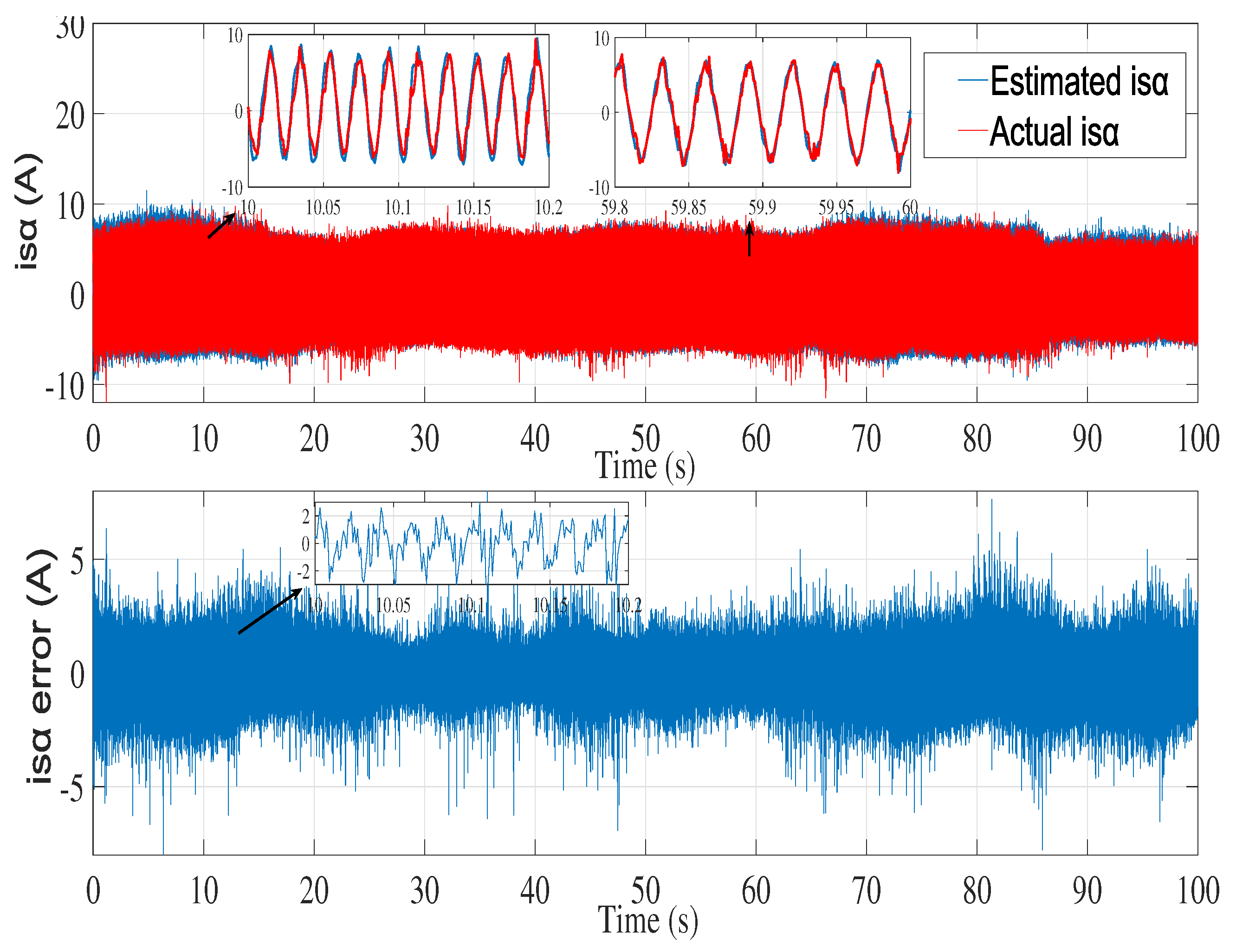
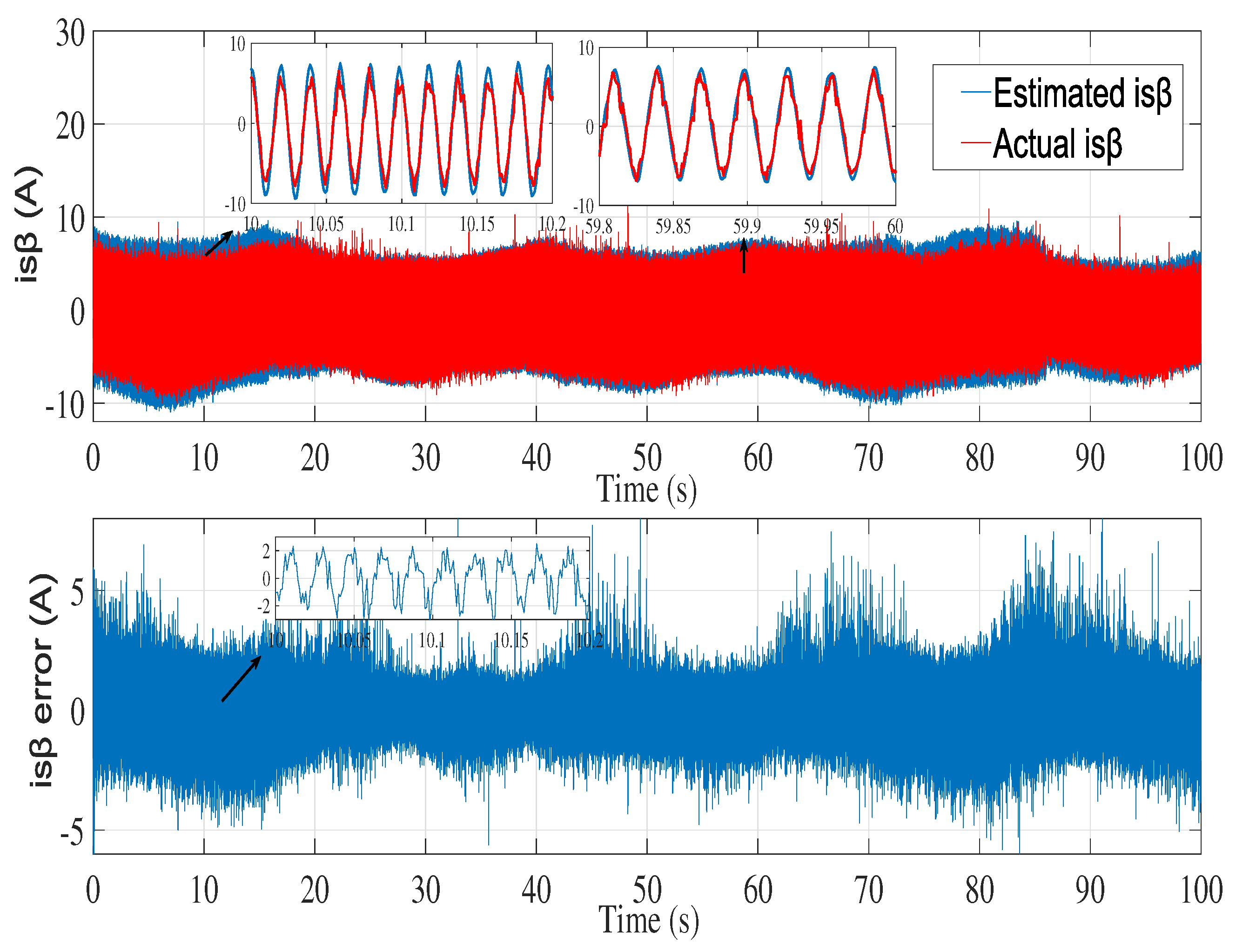
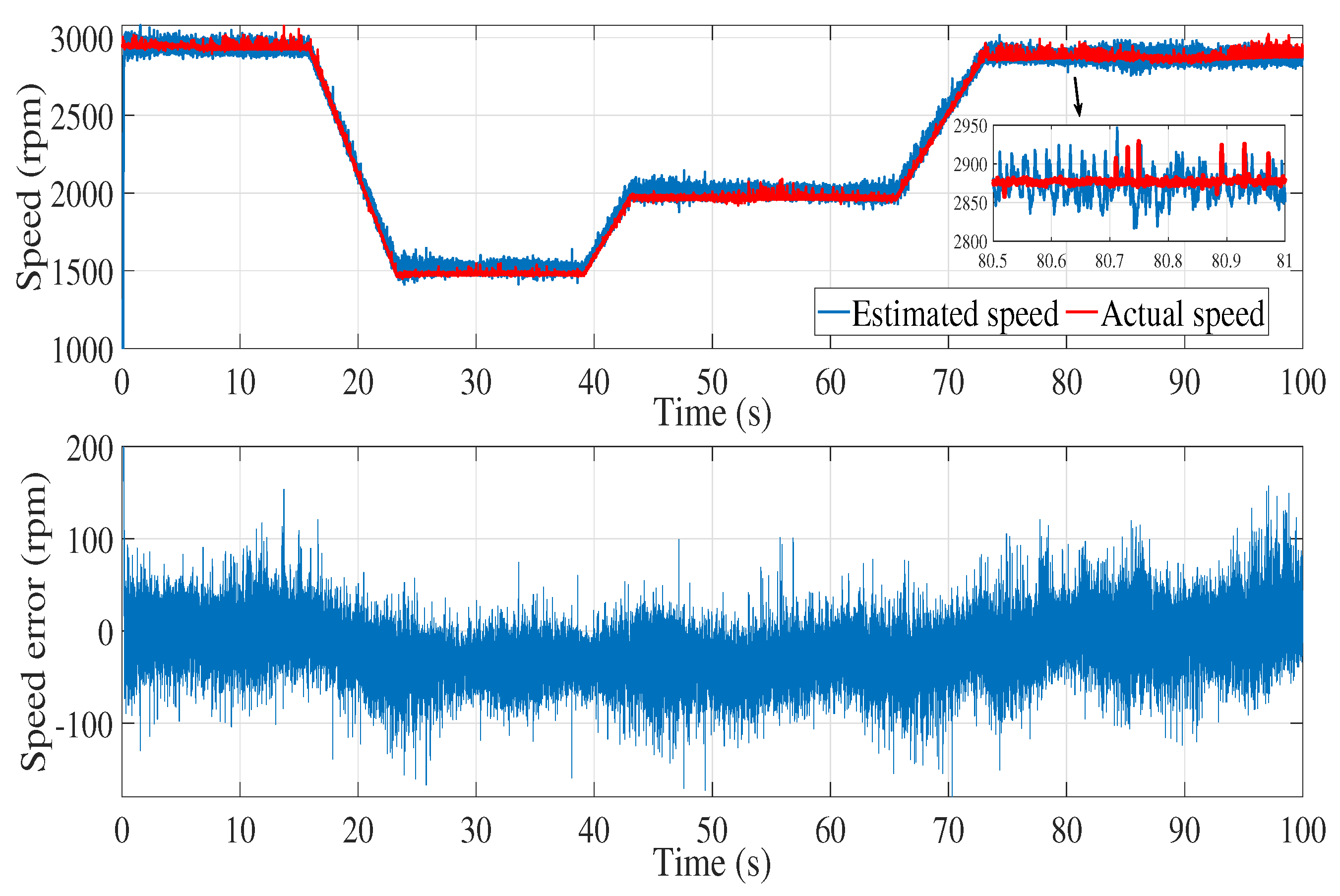
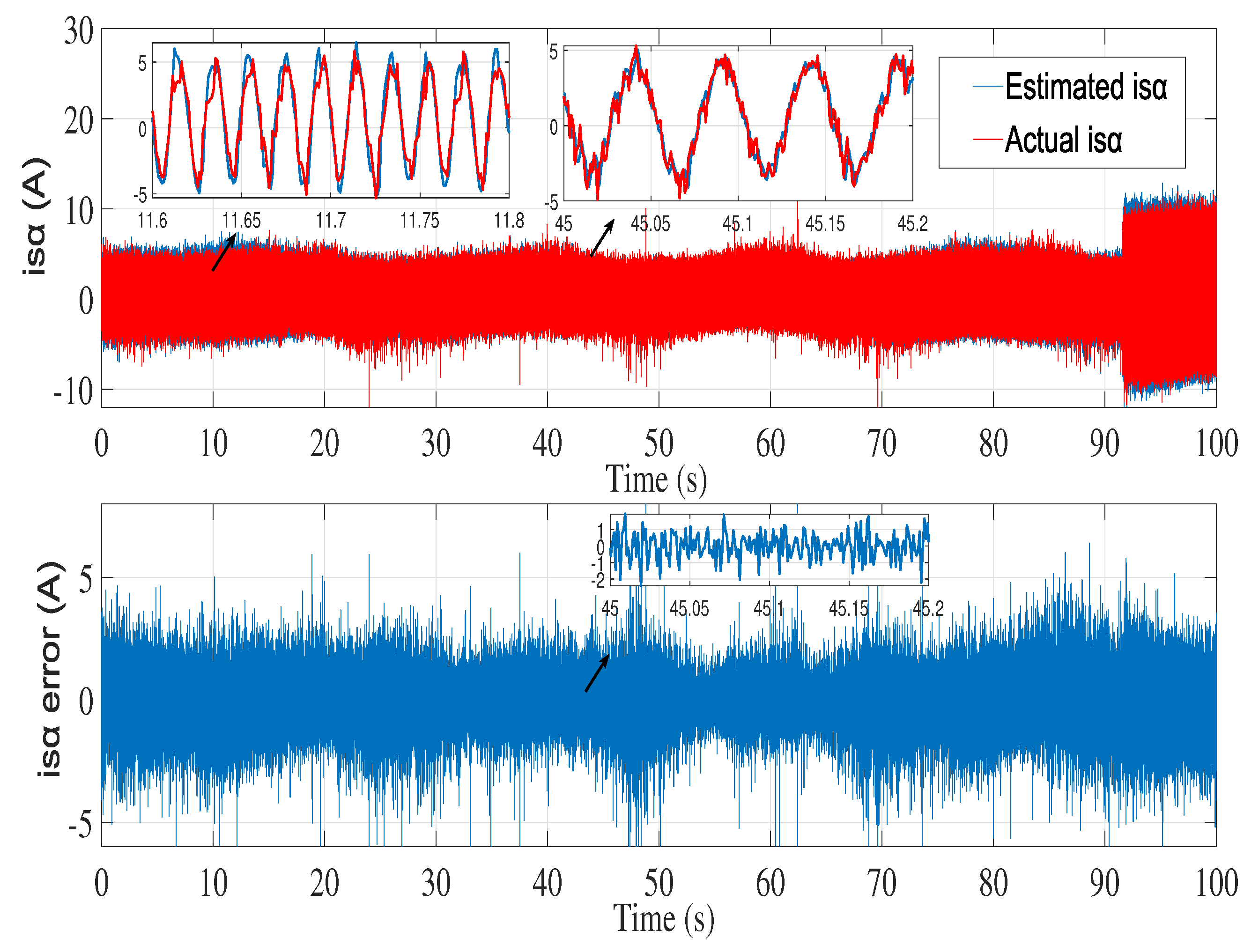
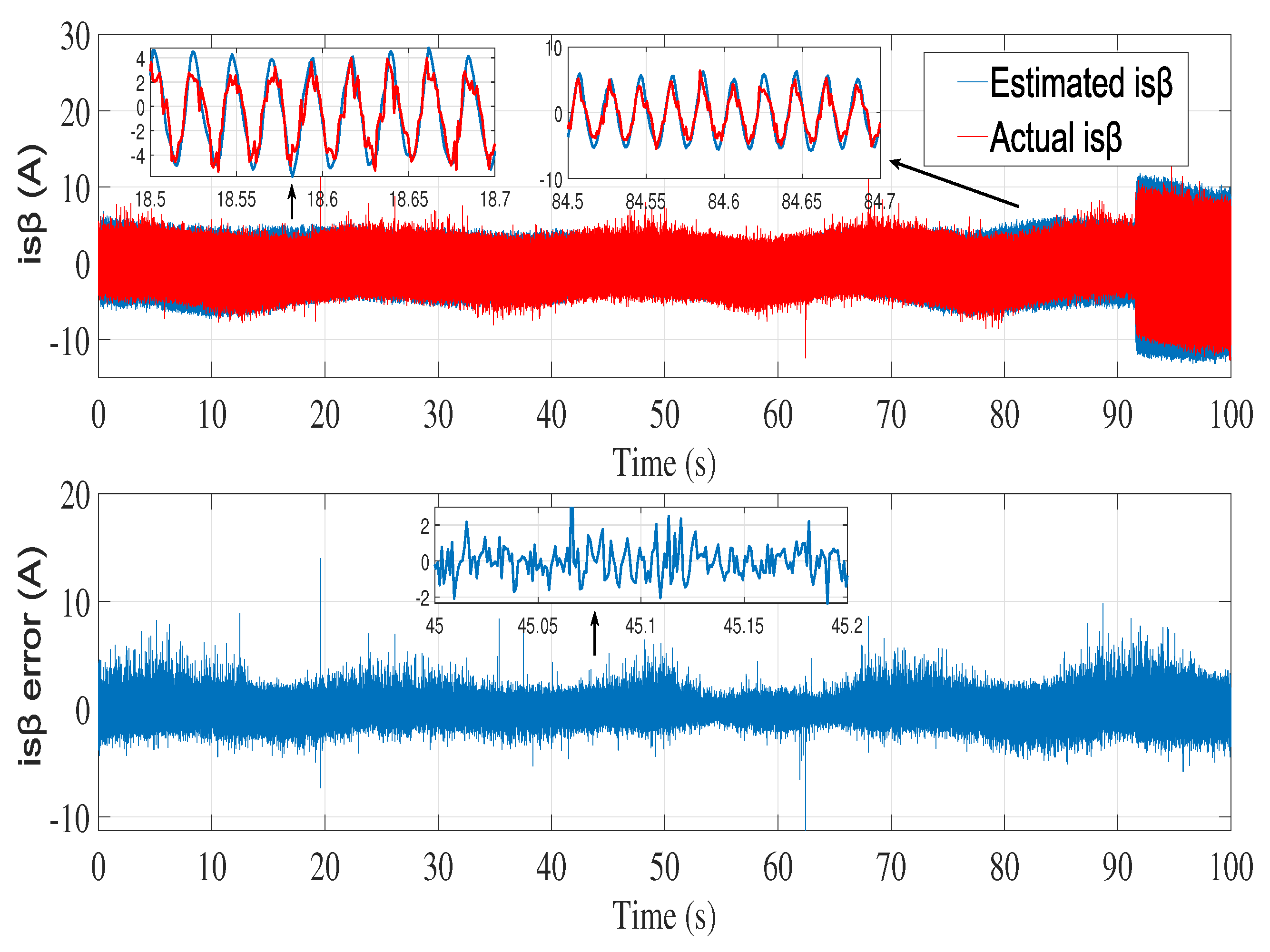
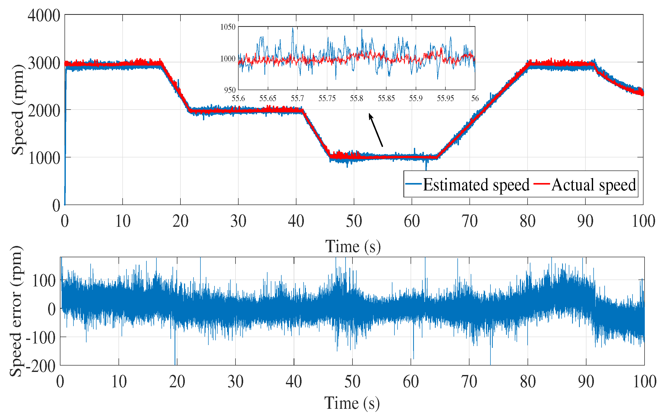
7. Conclusion

In this paper, a modified subspace model identification method is used to determine the noise covariance matrices of the EKF in order to estimate the IM rotor speed. The method involves exciting the voltages and currents using PRBS to estimate a discrete state space model of the IM. This model is then compared to the discrete-time state space representation involved in the Kalman filter equations. The resulted discrepancy is finally transformed into covariance matrix estimates. Because the subspace state space system identification requires an observable model, the 4^th order induction motor model is first identified. This model is then used to determine the system noise covariance matrices of the 5^th order model. These estimated matrices are finally used in the EKF algorithm to estimate the rotor speed. The method has been tested experimentally where accurate speed estimation has been obtained.

Acknowledgments

We would like to acknowledge the contributions of Chauvin Arnoux company to this project and their support in making this research possible in terms of resources and expertise. We are grateful for their commitment to advancing the objectives of this project and look forward to future collaborations.

References

Rashid, M.H. Power electronics handbook; Butterworth-heinemann, 2017.
Vieira, R.P.; Gastaldini, C.C.; Azzolin, R.Z.; Gründling, H.A. Sensorless sliding-mode rotor speed observer of induction machines based on magnetizing current estimation. IEEE Transactions on Industrial Electronics 2013, 61, 4573–4582. [Google Scholar] [CrossRef]
Accetta, A.; Cirrincione, M.; Pucci, M.; Vitale, G. Closed-loop MRAS speed observer for linear induction motor drives. IEEE Transactions on Industry Applications 2014, 51, 2279–2290. [Google Scholar] [CrossRef]
Kim, Y.R.; Sul, S.K.; Park, M.H. Speed sensorless vector control of induction motor using extended Kalman filter. IEEE Transactions on Industry Applications 1994, 30, 1225–1233. [Google Scholar]
Shi, K.; Chan, T.; Wong, Y.; Ho, S.L. Speed estimation of an induction motor drive using extended Kalman filter. In Proceedings of the 2000 IEEE Power Engineering Society Winter Meeting. Conference Proceedings (Cat. No. 00CH37077). IEEE; 2000; 1, pp. 243–248. [Google Scholar]
Shi, K.; Chan, T.; Wong, Y.; Ho, S.L. Speed estimation of an induction motor drive using an optimized extended Kalman filter. IEEE Transactions on Industrial Electronics 2002, 49, 124–133. [Google Scholar] [CrossRef]
Messaoudi, M.; Sbita, L.; Abdelkrim, M.N. EKF-Algorithm for Induction Motor State Estimation and Parameter Identification.
Barut, M.; Bogosyan, S.; Gokasan, M. Speed-sensorless estimation for induction motors using extended Kalman filters. IEEE Transactions on Industrial Electronics 2007, 54, 272–280. [Google Scholar] [CrossRef]
Osamah Basheer Noori, M.O.M. Flux and Speed Estimation of Induction Motors using Extended Kalman Filter. International Journal of Computer Applications 2018, 181, 0975–8887. [Google Scholar]
Aydin, M.; Gokasan, M.; Bogosyan, S. Fuzzy based parameter tuning of EKF observers for sensorless control of Induction Motors. In Proceedings of the 2014 International Symposium on Power Electronics, Electrical Drives, Automation and Motion. IEEE; 2014; pp. 1174–1179. [Google Scholar]
Yin, Z.; Xiao, L.; Sun, X.; Liu, J.; Zhong, Y. A speed and flux estimation method of induction motor using fuzzy extended kalman filter. In Proceedings of the 2014 International Power Electronics and Application Conference and Exposition. IEEE; 2014; pp. 693–698. [Google Scholar]
Yu, H.X.; Hu, J.T. Speed and load torque estimation of induction motors based on an adaptive extended Kalman filter. Advanced Materials Research 2012, 433, 7004–7010. [Google Scholar] [CrossRef]
Yin, Z.; Li, G.; Zhang, Y.; Liu, J.; Sun, X.; Zhong, Y. A speed and flux observer of induction motor based on extended Kalman filter and Markov chain. IEEE Transactions on Power Electronics 2016, 32, 7096–7117. [Google Scholar] [CrossRef]
Yin, Z.; Li, G.; Du, C.; Sun, X.; Liu, J.; Zhong, Y. An adaptive speed estimation method based on a strong tracking extended Kalman filter with a least-square algorithm for induction motors. Journal of Power Electronics 2017, 17, 149–160. [Google Scholar] [CrossRef]
Yin, Z.; Li, G.; Zhang, Y.; Liu, J. Symmetric-strong-tracking-extended-Kalman-filter-based sensorless control of induction motor drives for modeling error reduction. IEEE Transactions on Industrial Informatics 2018, 15, 650–662. [Google Scholar] [CrossRef]
Zerdali, E.; Barut, M. Extended Kalman filter based speed-sensorless load torque and inertia estimations with observability analysis for induction motors. Power Electronics and Drives 2018, 3, 115–127. [Google Scholar] [CrossRef]
Zerdali, E. Adaptive extended Kalman filter for speed-sensorless control of induction motors. IEEE Transactions on Energy Conversion 2018, 34, 789–800. [Google Scholar] [CrossRef]
Zerdali, E. strong tracking extended Kalman filter based speed and load torque estimations of induction motor. In Proceedings of the 2019 1st Global Power, Energy and Communication Conference (GPECOM). IEEE; 2019; pp. 216–221. [Google Scholar]
Zerdali, E.; Yildiz, R.; Inan, R.; Demir, R.; Barut, M. Improved speed and load torque estimations with adaptive fading extended Kalman filter. International Transactions on Electrical Energy Systems 2021, 31, e12684. [Google Scholar] [CrossRef]
Mussot, V.; Mercère, G.; Dairay, T.; Arvis, V.; Vayssettes, J. Noise covariance matrix estimation with subspace model identification for Kalman filtering. International Journal of Adaptive Control and Signal Processing 2021, 35, 591–611. [Google Scholar] [CrossRef]
Verhaegen, M.; Verdult, V. Filtering and system identification: a least squares approach; Cambridge university press, 2007.
Van Overschee, P.; De Moor, B. Subspace identification for linear systems: Theory—Implementation—Applications; Springer Science & Business Media, 2012.
Katayama, T.; et al. Subspace methods for system identification; Vol. 1, Springer, 2005.
Mercere, G. Regression techniques for subspace-based black-box state-space system identification: an overview. arXiv preprint, arXiv:1305.7121 2013.
Kailath, T.; Sayed, A.H.; Hassibi, B. Linear Estimation (Information and System Sciences Series). Technical report, Upper Saddle River, NJ: Prentice-Hall, 2000.
O’Rourke, C.J.; Qasim, M.M.; Overlin, M.R.; Kirtley, J.L. A geometric interpretation of reference frames and transformations: dq0, clarke, and park. IEEE Transactions on Energy Conversion 2019, 34, 2070–2083. [Google Scholar] [CrossRef]
Korkmaz, F. Performance improvement of induction motor drives with model-based predictive torque control. Turkish Journal of Electrical Engineering and Computer Sciences 2020, 28, 525–539. [Google Scholar] [CrossRef]
Böcker, J. Discrete-time model of an induction motor. European Transactions on Electrical Power 1991, 1, 65–71. [Google Scholar] [CrossRef]
Simon, D. Optimal state estimation: Kalman, H_∞ and nonlinear approaches; Hoboken, NJ: Wiley, 2006. [Google Scholar]
Peternell, K.; Scherrer, W.; Deistler, M. Statistical analysis of novel subspace identification methods. Signal Processing 1996, 52, 161–177. [Google Scholar] [CrossRef]

Figure 1. Single-phase equivalent circuit in the stationary reference frame.

Figure 2. Experimental system.

Figure 3.

i s_{α}

estimation using EKF tunned by a trial-and-error method-First test.

Figure 3.

i s_{α}

estimation using EKF tunned by a trial-and-error method-First test.

Figure 4.

i s_{β}

estimation using EKF tunned by a trial-and-error method-First test.

Figure 4.

i s_{β}

estimation using EKF tunned by a trial-and-error method-First test.

Figure 5. Motor speed estimation using EKF tunned by a trial and error method-First test.

Figure 6.

i s_{α}

estimation using EKF tunned by a trial and error method-Second test.

Figure 6.

i s_{α}

estimation using EKF tunned by a trial and error method-Second test.

Figure 8. Motor speed estimation using EKF tunned by a trial and error method-Second test.

Figure 9. Pseudo random binary sequence exciting the motor voltages and currents used in the subspace model identification.

Figure 10. The block diagram of experimental setup for noise covariance matrices estimation.

Figure 11. Actual and identified

i_{s α}

Figure 11. Actual and identified

i_{s α}

Figure 12. Actual and identified

i_{s β}

Figure 12. Actual and identified

i_{s β}

Figure 19. Estimation speed comparison between manual and automated EKF tuning.

Table 1. Mean squared error of estimated speed.

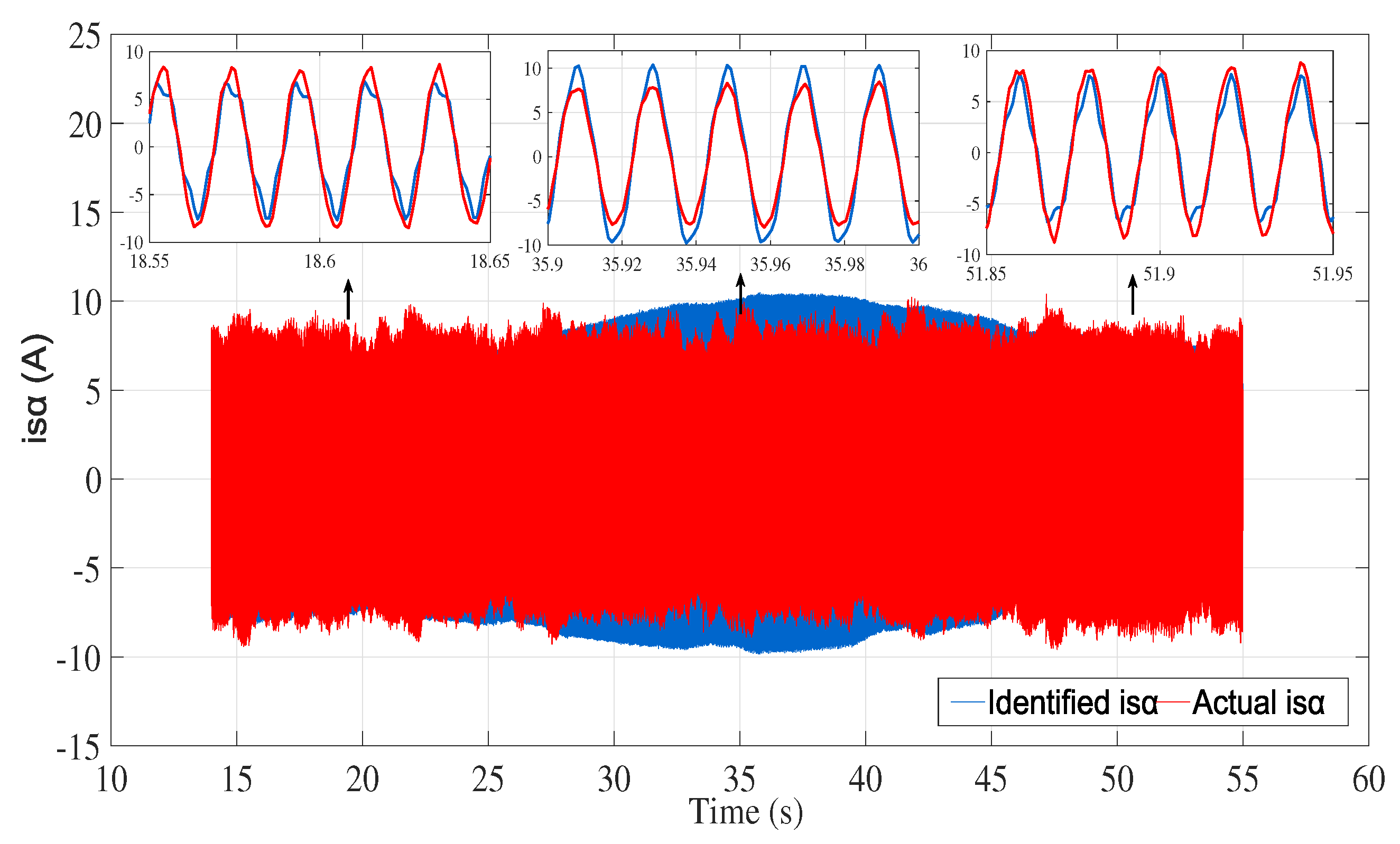
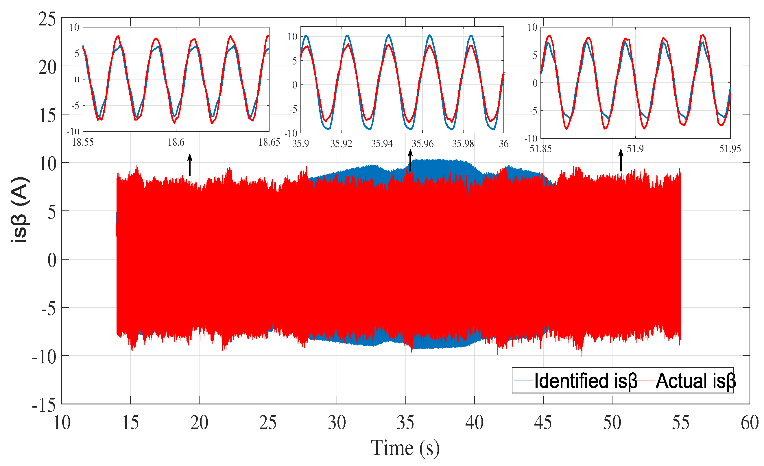
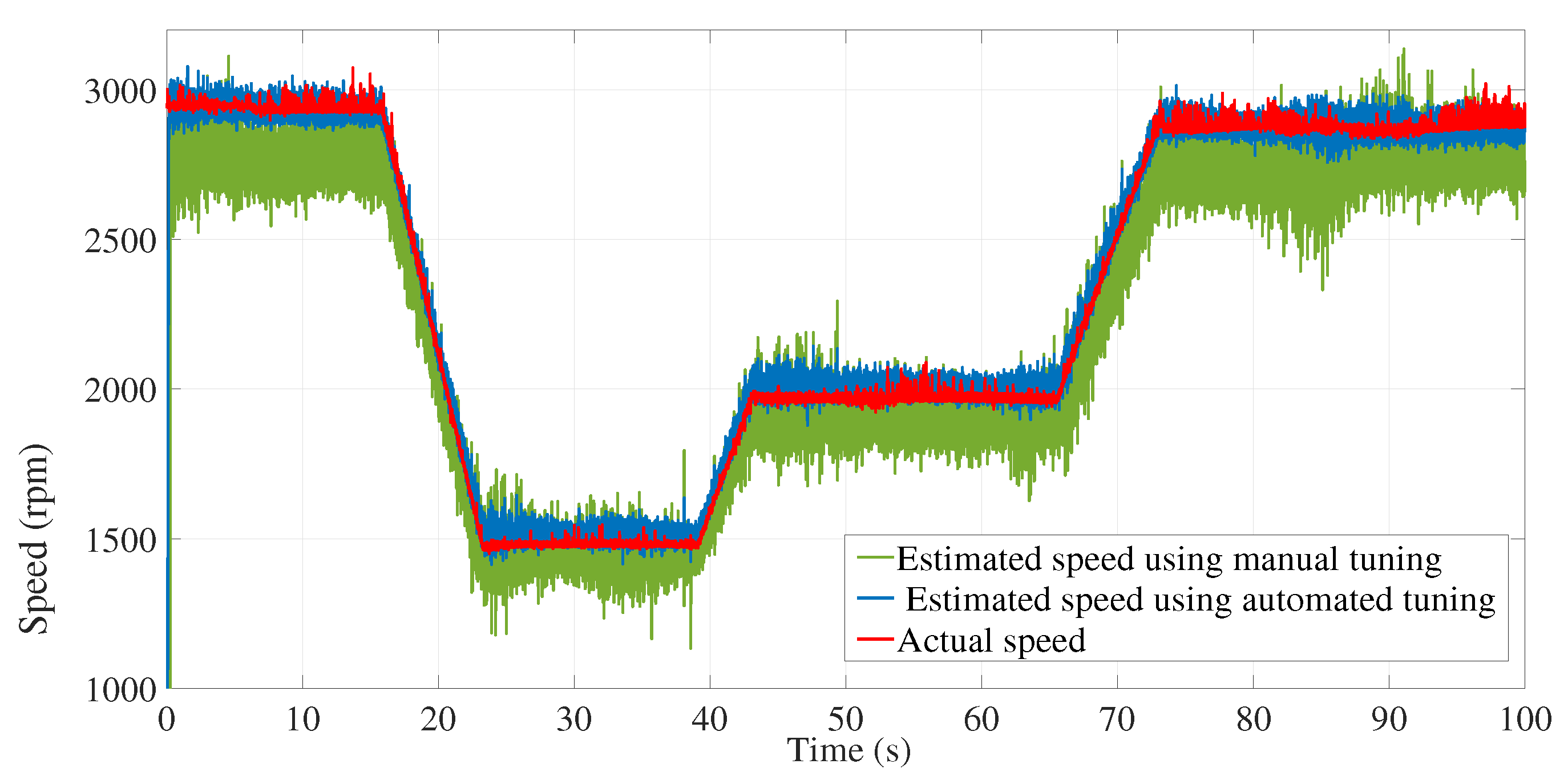
Disclaimer/Publisher’s Note: The statements, opinions and data contained in all publications are solely those of the individual author(s) and contributor(s) and not of MDPI and/or the editor(s). MDPI and/or the editor(s) disclaim responsibility for any injury to people or property resulting from any ideas, methods, instructions or products referred to in the content.

© 2024 by the authors. Licensee MDPI, Basel, Switzerland. This article is an open access article distributed under the terms and conditions of the Creative Commons Attribution (CC BY) license (http://creativecommons.org/licenses/by/4.0/).

Copyright: This open access article is published under a Creative Commons CC BY 4.0 license, which permit the free download, distribution, and reuse, provided that the author and preprint are cited in any reuse.