1. Introduction
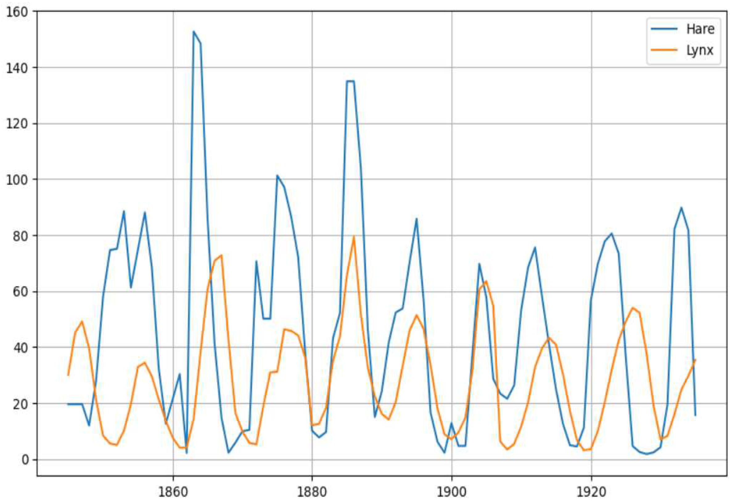
One of the major predators of the snowshoe hare is the Canadian lynx and on the other hand, snowshoe hares are one of the major food sources for the Canadian lynx. Over hundreds of years, they have hunted the hares and their populations show cyclic behaviors. This relationship in particular has been a basis for the prey predator models. Dynamical systems for prey-predator relationships is one of the topics which is of high interests in the field of mathematical ecology. One of the simplest models includes the model of Lotka Volterra which involves only one prey and one predator. The system can become more complicated as we start to consider more conditions which may include increasing the depth of the food chain or involving more than one preys or predators. Additionally, different functional responses also lead to varying models. The presence of the non linear dynamics in higher modifications of the prey predator models, leads to chaotic behavior which suggests the presence chaos in nature in large numbers. The paper is intended to provide a review on some of the models and their simulations which are closely related to the Lynx-Hare relationship.
2. Preliminary models
2.1. One prey One predator Model
The most basic model assumes exponential growth of the prey in the absence of the predator. In the case of the presence of a predator, the growth decreases naturally and the decline is dependent on both the populations of the prey and the predator as more prey implies more food for the predators implying rise in predator population, which in turn results in decline of prey population. The same idea holds true for the predator except the sign changes as more prey implies more food for the predators including its reproduction rate and further we will have to eliminate the death rate. Putting all the parameters in the form of equations, we will have the following system of equations for prey and predator population respectively.
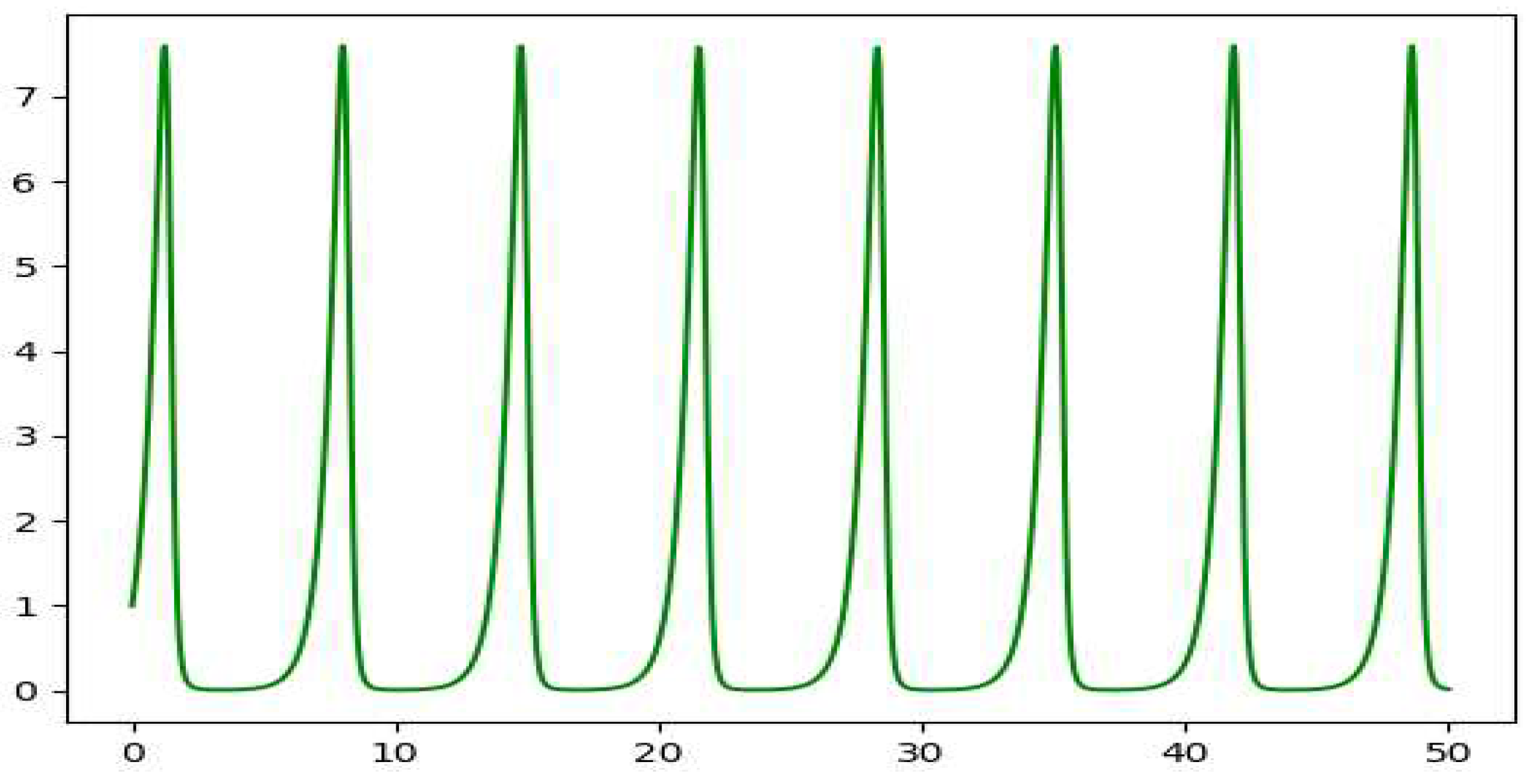
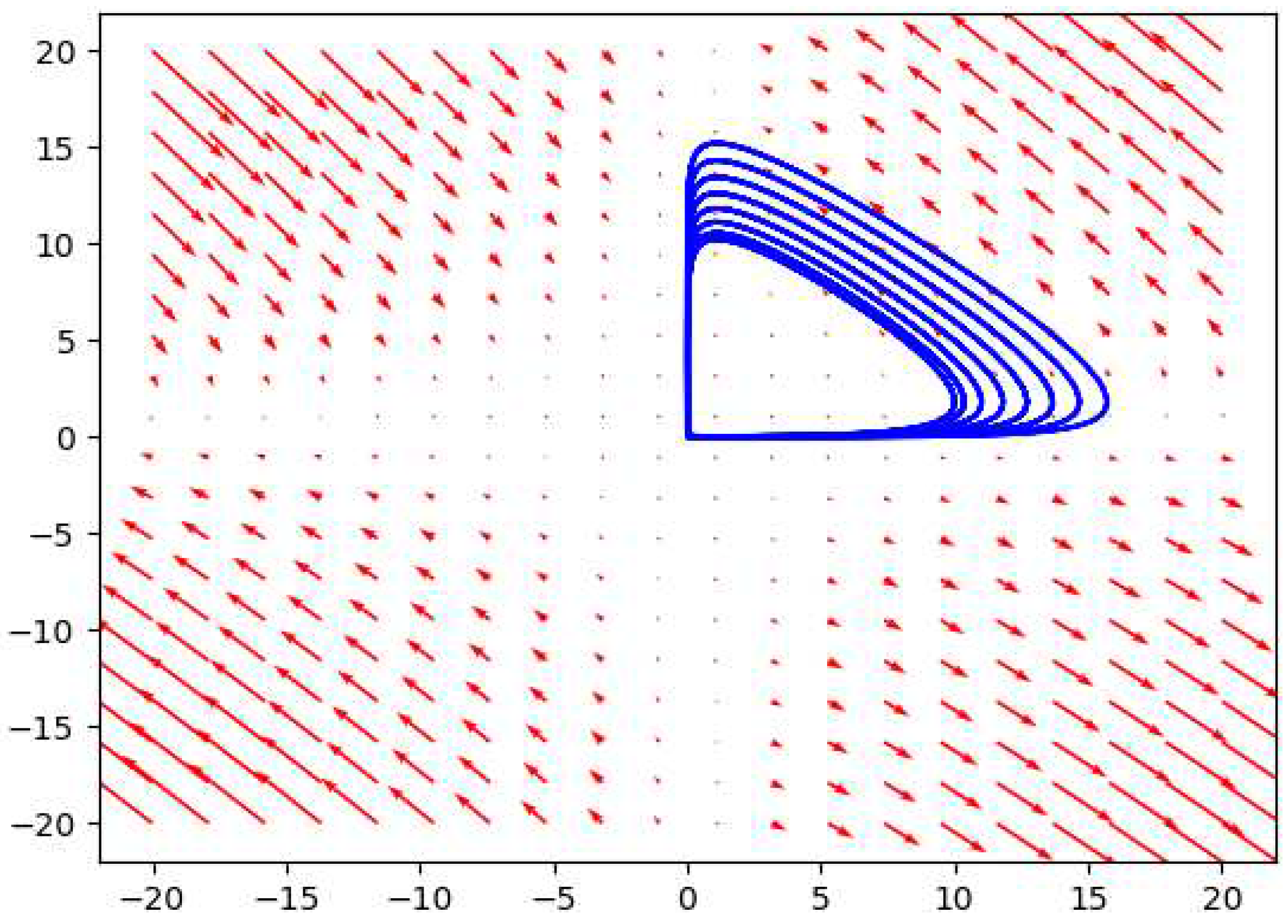
The plots we get on solving the equations are periodic which further implies the closed structure of the phase plot. Depending on the initial conditions, which in this case is the initial value of y, we get concentric closed figures around the equilibrium point in the phase, which in this case is a center (The equilibrium occurs when both ).
Figure 1.
The plot of x vs t on solving the Lotka Volterra equation.
Figure 1.
The plot of x vs t on solving the Lotka Volterra equation.
Figure 2.
The plot of y vs t on solving the Lotka Volterra equation.
Figure 2.
The plot of y vs t on solving the Lotka Volterra equation.
Figure 3.
The phase plot of y vs x on solving the Lotka Volterra equations.
Figure 3.
The phase plot of y vs x on solving the Lotka Volterra equations.
Table 1.
For the simulation we took the following values into consideration for equations 1 and 2.
Table 1.
For the simulation we took the following values into consideration for equations 1 and 2.
| Variables |
Values |
|
2 |
|
1.1 |
|
1 |
|
0.9 |
2.2. Modified Model
Volterra had given a general theory on species. For two species, the modified equations are
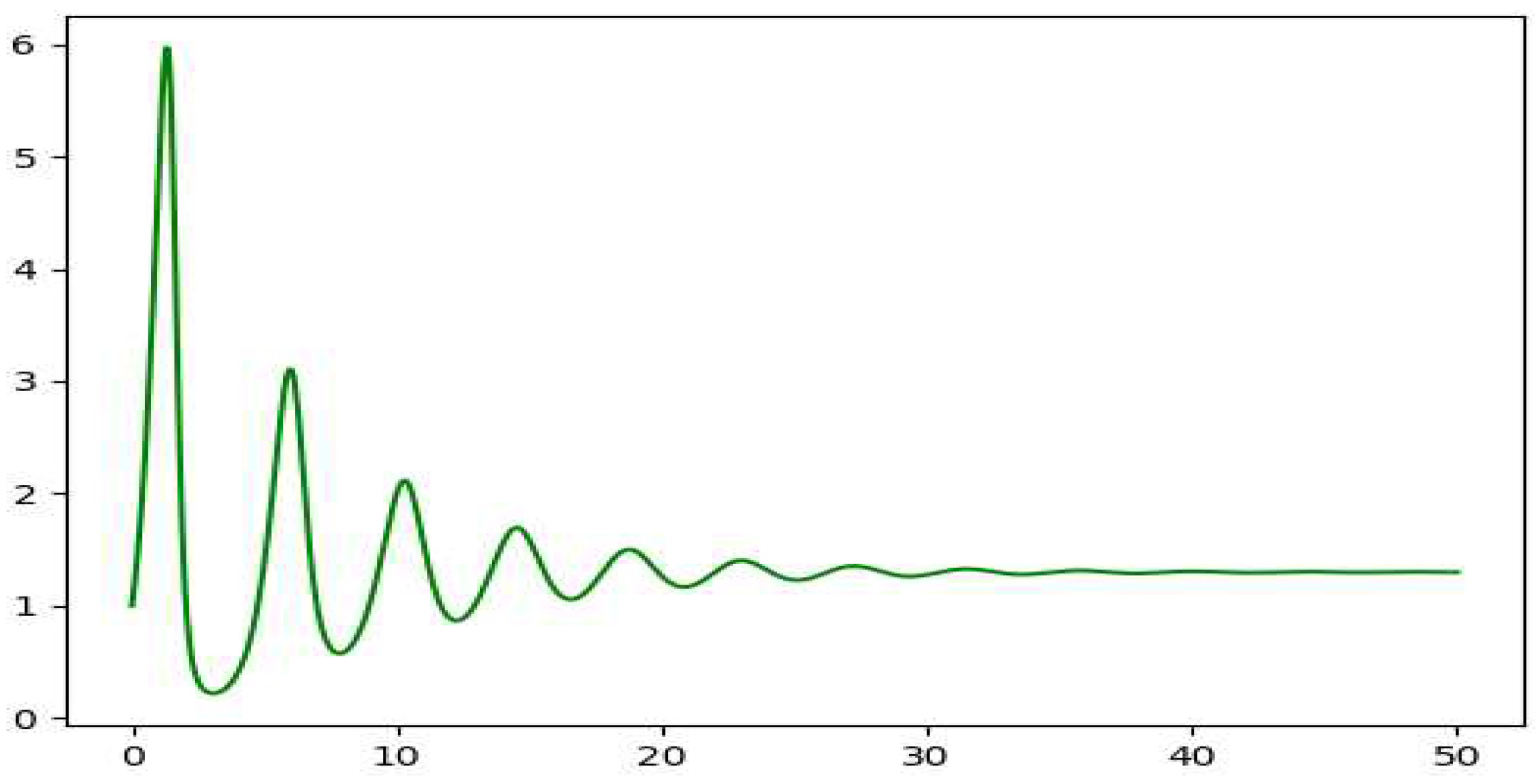
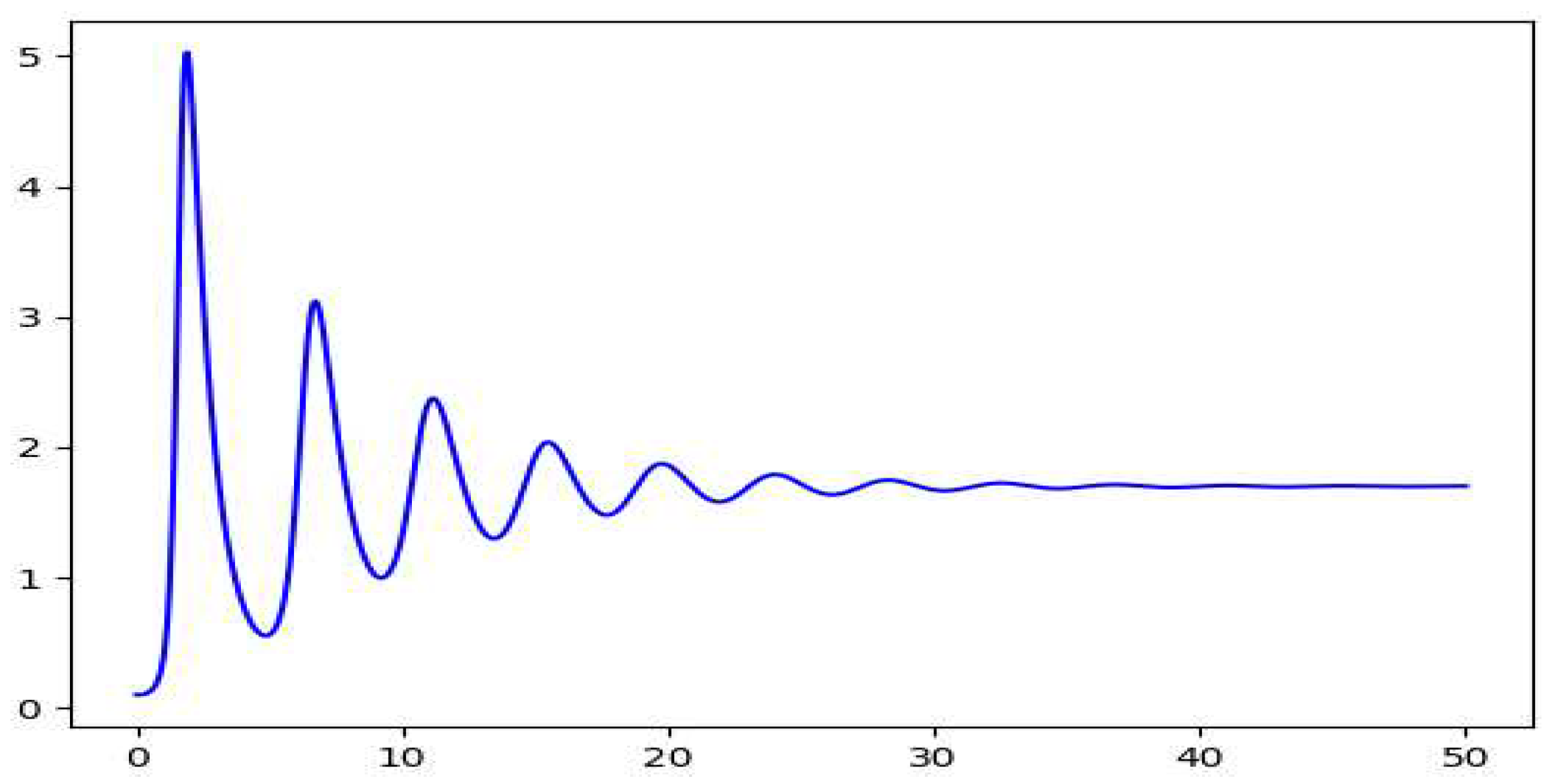
The plots we get for the same values for the variables additionally considering show damping plots. The phase plot we get on solving the equations is a spiral with focus at the equilibrium point. This gives us a damped oscillation of the populations for both the species. The equilibrium here forms a stable focus. The different spirals are for the different starting values of y.
Figure 4.
The plot of x vs t on solving the modified Lotka Volterra equation.
Figure 4.
The plot of x vs t on solving the modified Lotka Volterra equation.
Figure 5.
The plot of y vs t on solving the modified Lotka Volterra equation.
Figure 5.
The plot of y vs t on solving the modified Lotka Volterra equation.
Figure 6.
The plot of x vs t on solving the modified Lotka Volterra equation.
Figure 6.
The plot of x vs t on solving the modified Lotka Volterra equation.
2.3. Depth three prey predator model
The depth three food chain includes one predator, one prey and a lowest level species which is fed on by the prey. This may include producers like carrots for food chains like Fox → Rabbit → Carrots. Simple models considering functional responses for both species have been studied before. Incorporating type II functional responses for both the prey and the predator, and considering logistic growth of the lowest level in the absence of the prey, we get the following model.
where
The parameters can be reduced which will further give us the equations
where
considering the reductions
Table 2.
The authors set the values, with the intention to consider biologically reasonable food chain and check if chaotic behaviors are likely to exist for the equations 8, 9 and 10.
Table 2.
The authors set the values, with the intention to consider biologically reasonable food chain and check if chaotic behaviors are likely to exist for the equations 8, 9 and 10.
| Variables |
Values |
|
5.0 |
|
2.0 to 6.0 |
|
0.1 |
|
2.0 |
|
0.4 |
|
0.01 |
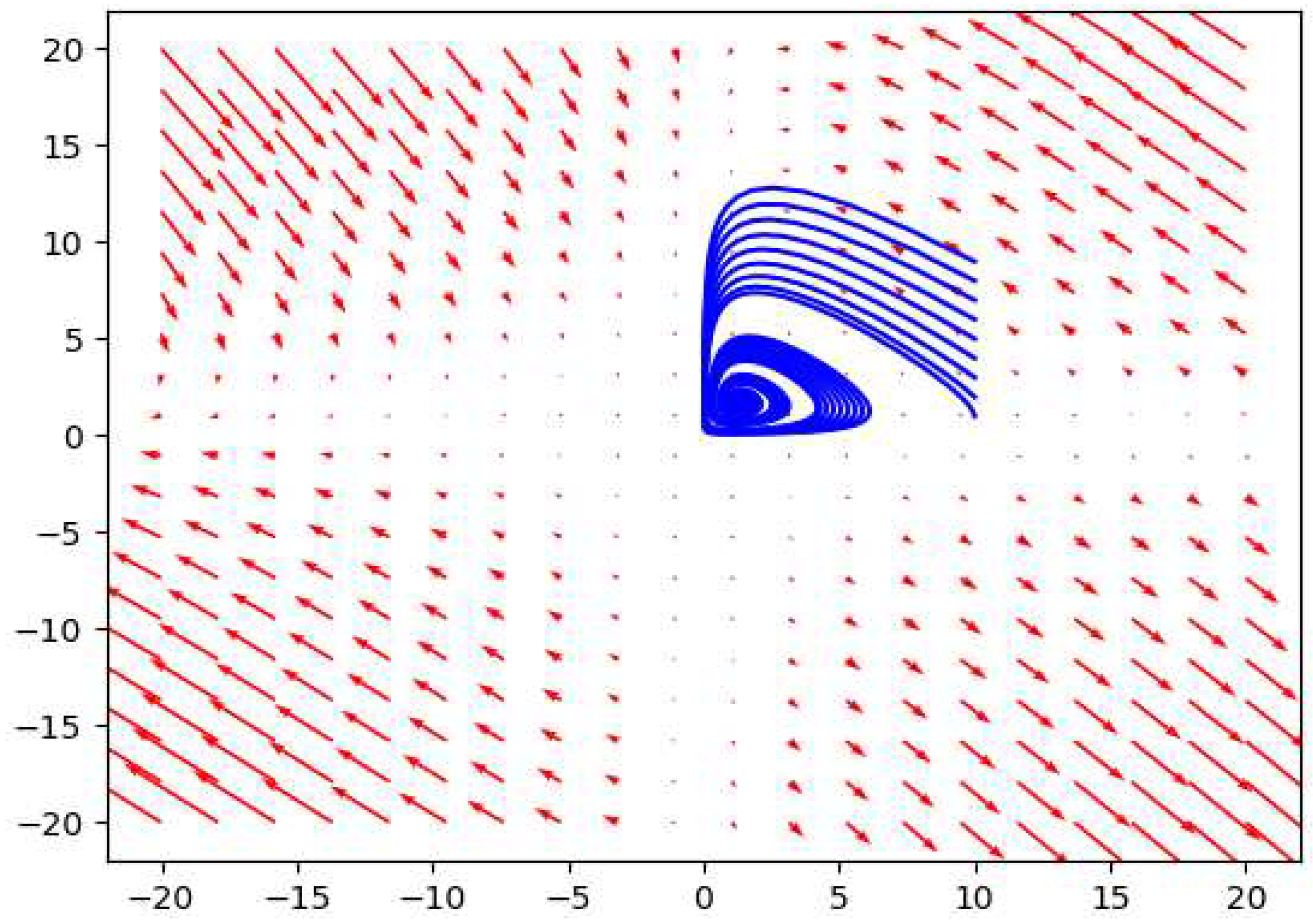
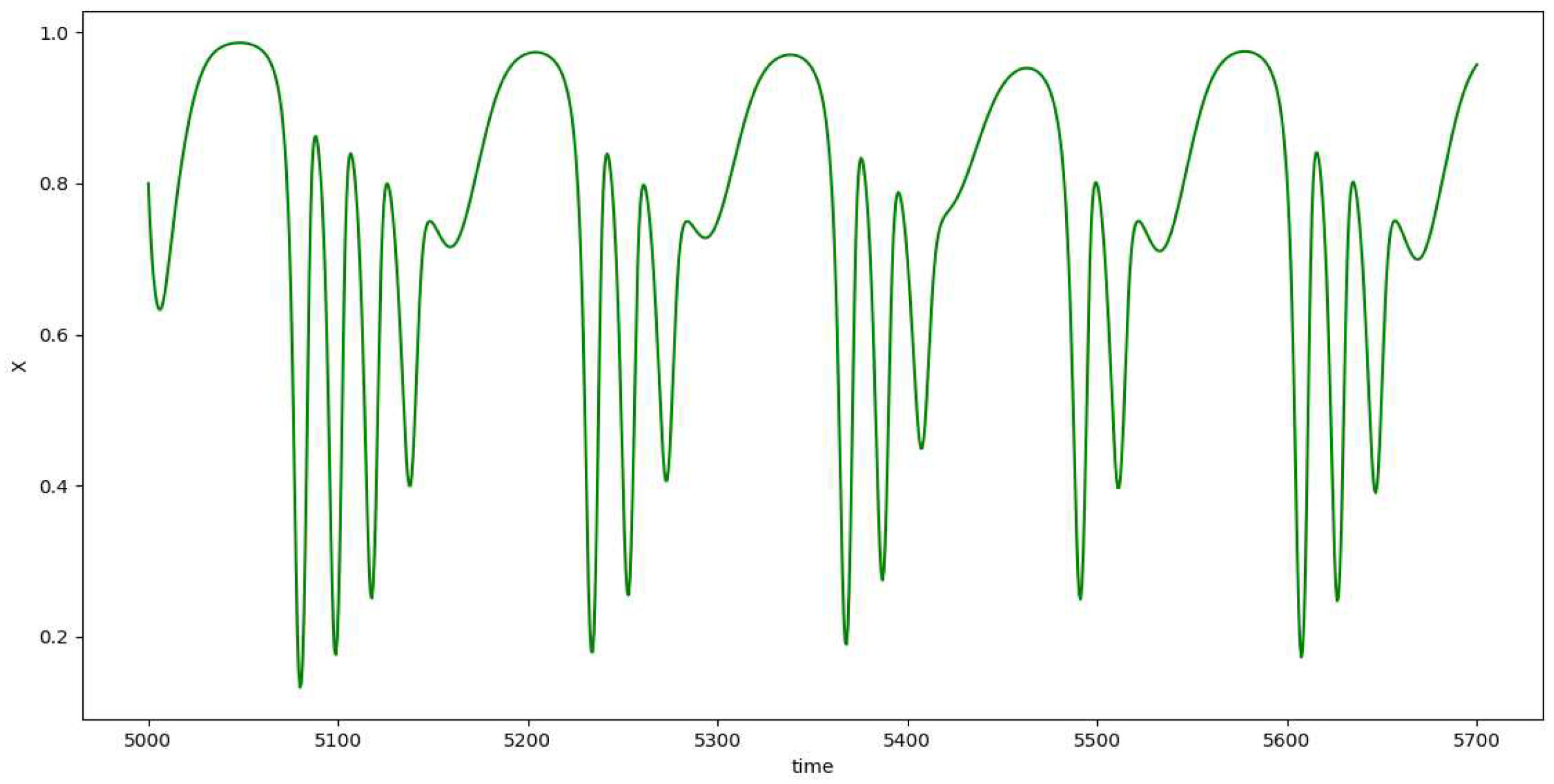
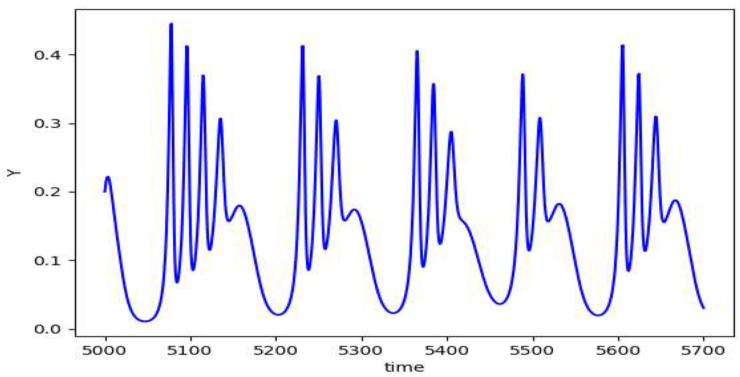
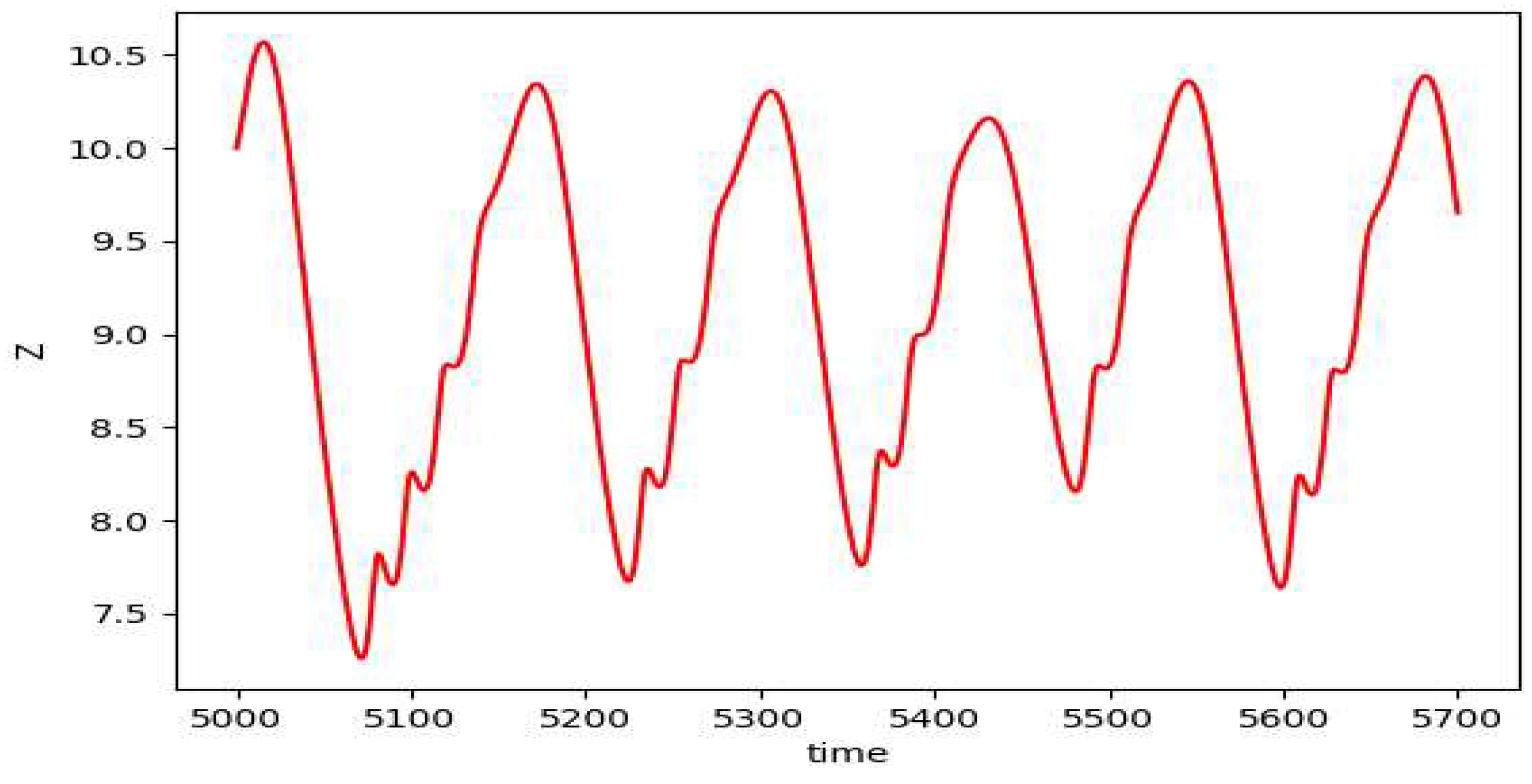
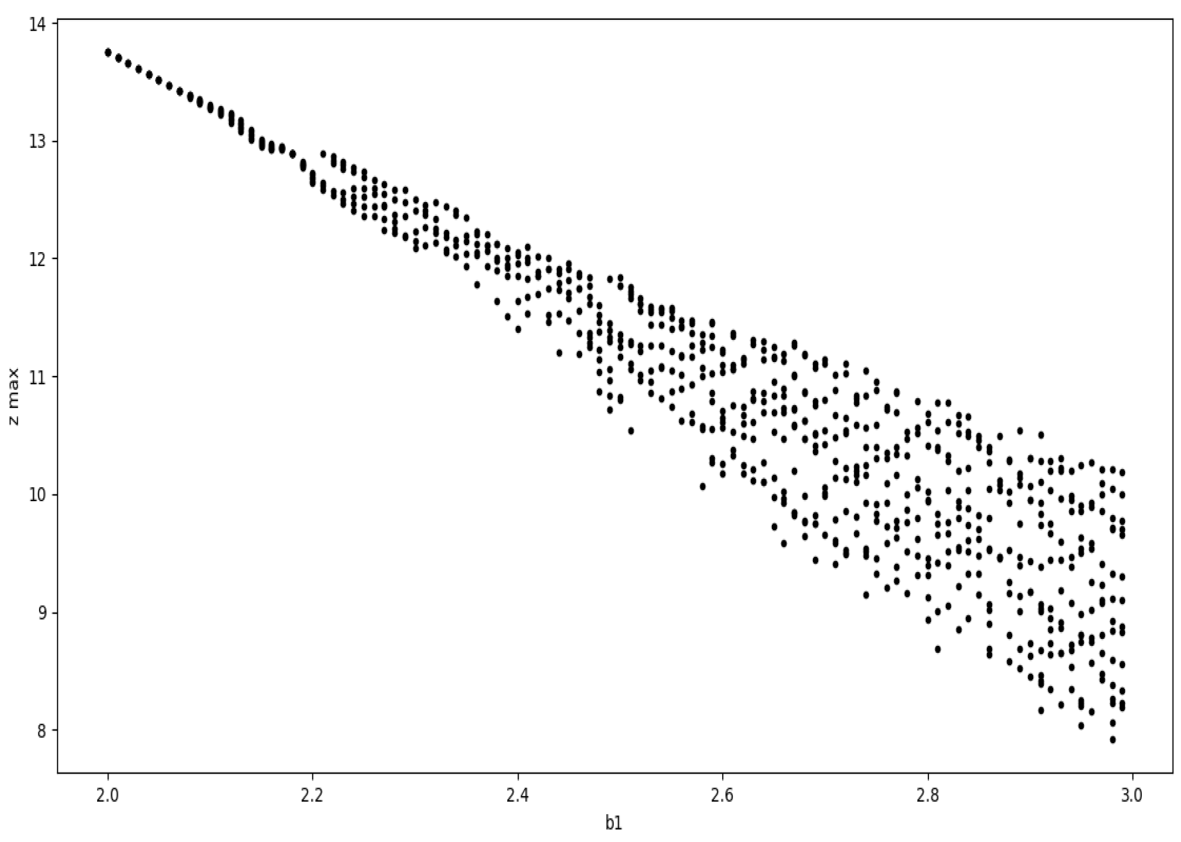
Although we get to see some kind of cyclic plots, the nonuniform behavior of the plots suggests chaotic nature of the model. On varying the value of
, we start to observe chaos. The plot of the peak value of
z against the values of
gives us the bifurcation diagram as in
Figure 10.
Figure 7.
The plot of x vs t for the depth 3 prey predator model.
Figure 7.
The plot of x vs t for the depth 3 prey predator model.
Figure 8.
The plot of y vs t for the depth 3 prey predator model.
Figure 8.
The plot of y vs t for the depth 3 prey predator model.
Figure 9.
The plot of z vs t for the depth 3 prey predator model.
Figure 9.
The plot of z vs t for the depth 3 prey predator model.
Figure 10.
The plot of the peak value of z in each cycle against for the depth 3 prey predator model.
Figure 10.
The plot of the peak value of z in each cycle against for the depth 3 prey predator model.
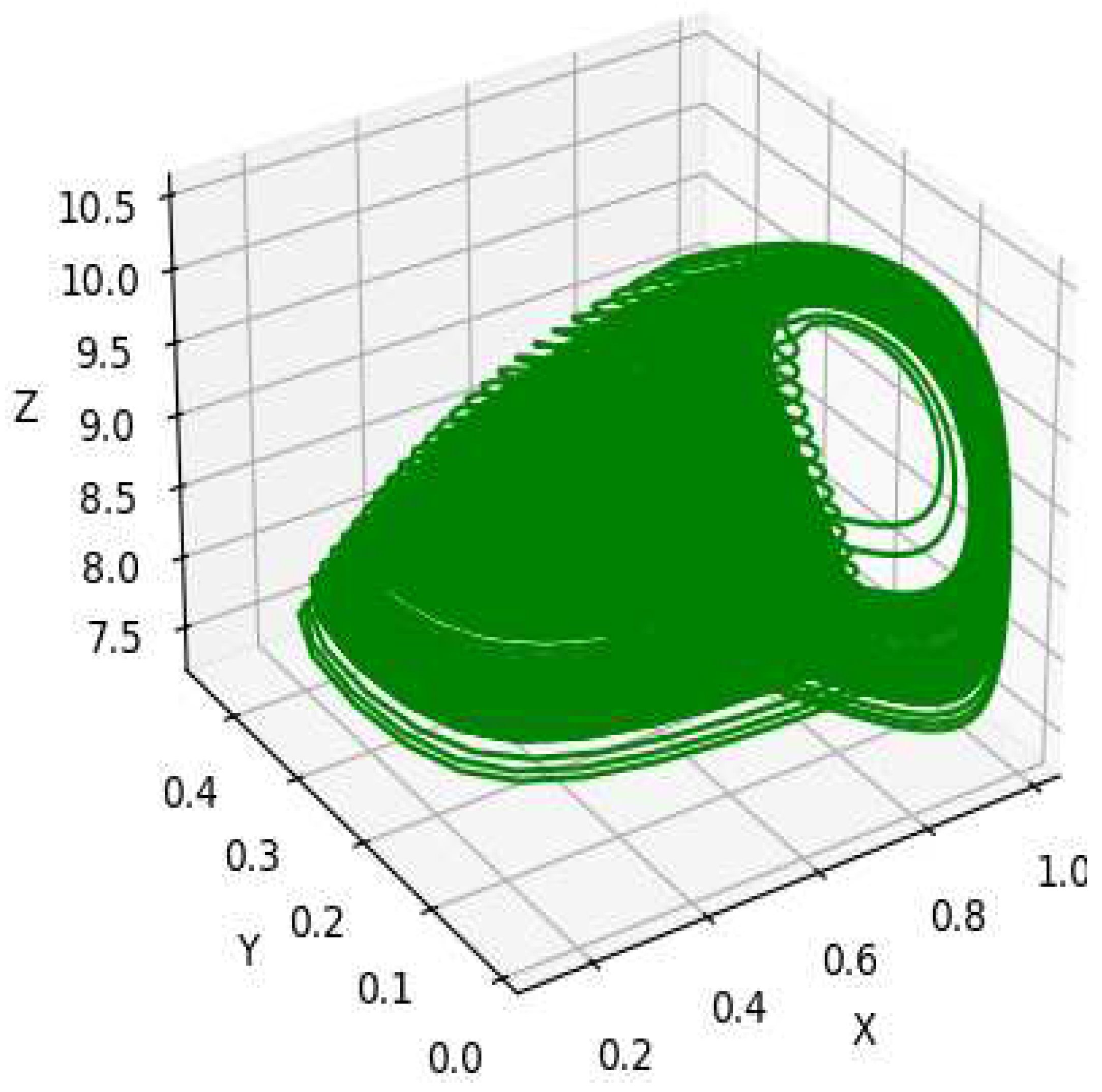
Figure 11.
The phase plot for the depth 3 prey predator model considering .
Figure 11.
The phase plot for the depth 3 prey predator model considering .
2.4. Two or more Predators and One prey model
The authors consider a modified model for the two predator one prey system, considering the Leslie Gower equations with Holling type I functional response. The equations are
However the authors of [3] consider a different model ( Hanski and Korpimaki), considering three predators for the Snowshoe Hares, Lynx, Coyote and Great Horned Owl. The plots for this model are according to the given values in
Table 3. The authors suggest the following model for single prey-predator relationship
which can be generalized for arbitrary number of predators as
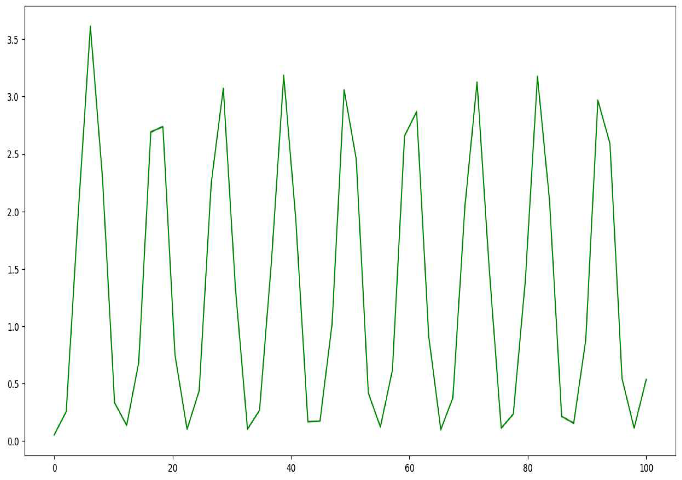
Figure 12.
The plot of Hare population for the model in equations 20 and 21.
Figure 12.
The plot of Hare population for the model in equations 20 and 21.
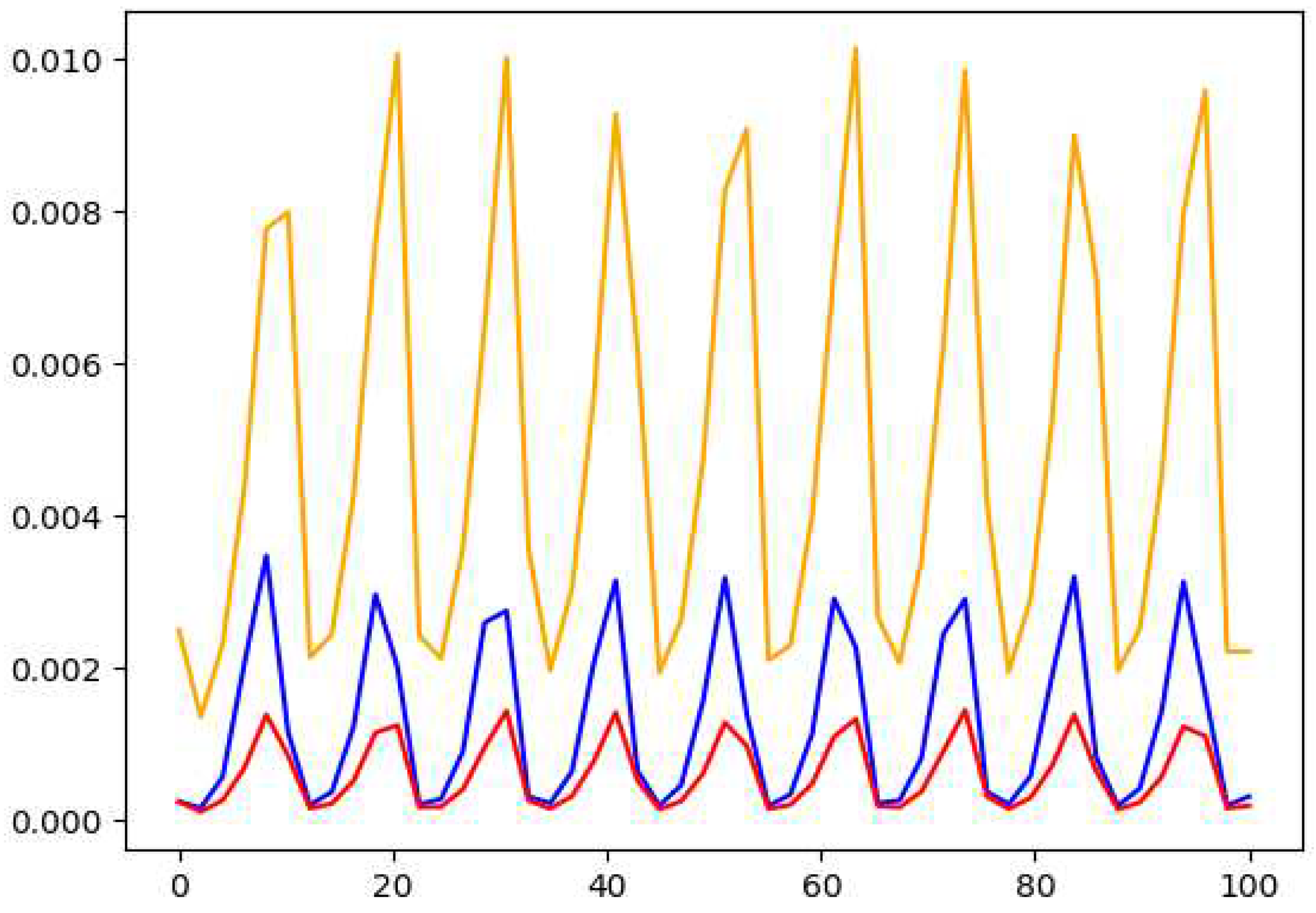
Figure 13.
The plots of Horned owl (yellow), coyote (red) and lynx (blue) for the model in equations 20 and 21.
Figure 13.
The plots of Horned owl (yellow), coyote (red) and lynx (blue) for the model in equations 20 and 21.
3. Canadian Lynx-Snowshoe Hares population data
Although a major chunk of the food for the Canadian Lynx consists of snowshoe hares, the lynx also feeds on other preys and further hares are being preyed on by other predators like owls and coyotes. This entire system therefore can turn quite complex. We observed that chaos can occur considering depth three food chain, which in this case is relevant as the hares also feed on vegetations. Although the models suggest the cyclic behavior of the population dynamics, the exact reason for the 10 year cyclic nature of the population remains as a topic of debate. The theory that the hare-lynx cycle is a model example of a prey-predator oscillation has been challenged (Krebs 2001), while Trostel et al. (1987) contend that predation may be at least partially to blame for the cycle of snowshoe hares. According to May (1973), an illustration of a Lotka-Volterra oscillation is the population oscillation of hares and lynxes in Hudson Bay. But Leigh (1968) and Gilpin (1973) discovered that the hare-lynx dynamic is not an oscillation between prey and predator. The authors of [1] also claim to have not found any significant predation effect and they suggest that the rate of growth of hares and lynx as self-regulated or density dependent. Authors in [5] suggest that the Hare cycles appear to be most likely to be caused by three key factors: food, predation, and social interactions. The authors of [5] suggest a two factor explanation for the fluctuations in the amplitude of the cycles. A possible explanation for amplitude dampening being the migration of predators from areas with an increasing amplitude cycle to areas with a dampening one and the three assumptions according to the plant-quality model of Liu et al. (2012).
4. Conclusion
In this paper we have discussed about the Lotka-Volterra Model which considers only two species, the prey and the predator which gives us periodic plots. A modified version of the model does not consider indefinite increase of the prey in the absence of the predator. This gave a damping plot, where both the populations reach a certain equilibrium. The depth three food chain additionally includes vegetation on which the preys feed. Considering the Holling type II functional response for both the prey and the predator, we get to see a chaotic behavior in the dynamics. We finally considered the case of many predators and single prey, potraying two models. The relationship between Canadian Lynx and the snowshoe hares is a point of interest for ecologists. A variety of models are being proposed to suit the chaotic behaviors.
References
- Zhang, Zhibin & Tao, yi & Li, Zhenqing. (2007). Factors affecting hare lynx dynamics in the classic time series of the Hudson Bay Company, Canada. Climate Research. 34. 83-89. [CrossRef]
- Hastings, A., & Powell, T. (1991). Chaos in a three-species food chain. Ecology, 72(3), 896-903. [CrossRef]
- Tyson, R., Haines, S., & Hodges, K. E. (2010). Modelling the Canada lynx and snowshoe hare population cycle: the role of specialist predators. Theoretical Ecology, 3, 97-111. [CrossRef]
- Savitri, D., Suryanto, A., & Kusumawinahyu, W. M. (2019, June). A dynamics behaviour of two predators and one prey interaction with competition between predators. In IOP Conference Series: Materials Science and Engineering (Vol. 546, No. 5, p. 052069). IOP Publishing.
- harles J. Krebs, Rudy Boonstra, Stan Boutin, A.R.E. Sinclair, What Drives the 10-year Cycle of Snowshoe Hares? The ten-year cycle of snowshoe hares—one of the most striking features of the boreal forest— is a product of the interaction between predation and food supplies, as large-scale experiments in the yukon have demonstrated, BioScience, Volume 51, Issue 1, January 2001, Pages 25–35. [CrossRef]
- Krebs, Charles & Bryant, John & Kielland, Knut & Donoghue, Mark & Doyle, Frank & Carrière, Suzanne & Difolco, Donna & Berg, Nathan & Boonstra, Rudy & Boutin, Stan & Kenney, Alice & Reid, Donald & Bodony, Karin & Putera, Judy & Timm, Henry & Burke, Toby & Maier, Julie & Golden, Howard. (2014). ARTICLE What factors determine cyclic amplitude in the snowshoe hare (Lepus americanus) cycle?. Canadian Journal of Zoology. 92. 1039-1048. [CrossRef]
- Liu, R., Gourley, S.A., DeAngelis, D.L., and Bryant, J.P. 2012. Modeling the dynamics of woody plant–herbivore interactions with age-dependent toxicity. J. Math. Biol. 65(3): 521–552. [CrossRef] [PubMed]
- Stenseth, N. C., Falck, W., Bjørnstad, O. N., & Krebs, C. J. (1997). Population regulation in snowshoe hare and Canadian lynx: asymmetric food web configurations between hare and lynx. Proceedings of the National Academy of Sciences, 94(10), 5147-5152. [CrossRef]
|
Disclaimer/Publisher’s Note: The statements, opinions and data contained in all publications are solely those of the individual author(s) and contributor(s) and not of MDPI and/or the editor(s). MDPI and/or the editor(s) disclaim responsibility for any injury to people or property resulting from any ideas, methods, instructions or products referred to in the content. |
© 2024 by the authors. Licensee MDPI, Basel, Switzerland. This article is an open access article distributed under the terms and conditions of the Creative Commons Attribution (CC BY) license (http://creativecommons.org/licenses/by/4.0/).
