
Submitted:
17 January 2024
Posted:
17 January 2024
You are already at the latest version
Abstract
Modelling diameter distribution is an integral part of forest management. It requires the use of a suitable probability density function or cumulative distribution function with the appropriate fitting method. In this study, we compared the suitability of eight probability density functions fitted by derivative and optimization methods used for diameter distribution estimation of forest stands. The derivation and optimization were used on A Charlier, beta, generalized beta, gamma, Gumbel, Johnson’s SB, and Weibull (2 and 3-parameter). We used data from 167 permanent sample plots from Atlantic forest (Quercus robur) and 59 temporary sample plots from tropical forests (Tectona grandis). The quality of the fits was evaluated with different indices such as Kolmogorov–Smirnov, Cramer-von Mises, mean absolute error, bias and mean squared error. The results showed Johnson’s SB function was more suitable for describing the diameter distribution of the stands. Johnson’s SB, 3-parameter Weibull and generalized beta had consistent performance regardless of the fitting methods. The quality of fits produced by gamma, Gumbel and 2-parameter Weibull was poor.
Keywords:
Johnson’s SB
; Weibull
; generalized beta
; parameter estimation
; Quercus robur
; Tectona grandis
1. Introduction
Tree diameter distribution is an important component of forest management which is used for decision-making such as what and when to harvest, and what silvicultural treatment to apply [1,2]. Researchers can deduce details about the dynamics of forests, including recruitment rates, mortality patterns, and growth rates, by examining changes in diameter distributions across time [3]. Based on the diameter class model, we can assess a stand's stability, volume production, assortment structure, and maturity [4,5]. Thus, making it an important component in decision-support systems.
To estimate stand characteristics and their structures with a diameter class model, researchers rely on the use of a probability density function (PDF) or its cumulative form (CDF). Various probability density functions have been adopted in describing stem frequency in both natural forest stands and forest plantations such as beta [2,6,7], generalized beta [7,8], gamma [9,10,11], Johnson’s SB [12,13], Weibull [7,14,15,16], etc. with different levels of success. To date, the Weibull, gamma, beta and Johnson’s SB functions are the traditional functions commonly used in quantitative forestry. Other important functions like the Charlier (type A) have gained less importance. Besides the earlier work of Schnur [17] on the diameter distribution of Loblolly pine (Pinus taeda L), few and old published studies have been documented in forestry literature on the Charlier function to the best of our knowledge.
In forestry, the functions can be fitted using either the derivative methods and/or numerical optimization [7]. One advantage of the derivative methods is their simplicity and ease of estimation, which is obtained from stand characteristics [12,18,19,20]. However, it is difficult to quantify the uncertainty in the parameter estimates with derivative methods [7]. On the other hand, the uncertainty in the parameter estimates from optimization could be determined through the hessian matrix [21]. The Weibull function has been fitted by derivative methods such as moments and percentiles, and optimization to mixed spruce-fir stands [22], and tropical and Atlantic forests [7]. Recently, the same methods were used for the Weibull function to characterise the diameter distribution of European beech (Fagus sylvatica L.) [23]. The gamma function has been fitted by moments [10,11] and optimization [7]. The beta function has been fitted by the method of moments [2,7,24]. The generalized beta has been fitted by moments [7,8] and optimization [7]. The traditional methods for fitting Johnson’s SB function also include conditional maximum likelihood, moments, mode and percentiles, and optimization method by maximum likelihood [7].
Therefore, the main objective of this study was to compare the precision of A Charlier, Gumbel, gamma-2P, Weibull (2P and 3P), beta, generalized beta and Johnson’s SB functions fitted by a derivative method (Moments) and a numerical optimization method (MLE). We used data from two broadleaf species of even-aged stands in Atlantic and tropical forests.
2. Materials and Methods
2.1. Data set
The data used were obtained from a total of 167 permanent research plots (PRPs) in even-aged pedunculate oak (Quercus robur L.) stands throughout Galicia (northwest Spain) and 59 temporary sample plots (TSPs) in plantations of teak (Tectona grandis L. f.) in Omo and Gambari (south Nigeria). The size of the plots ranged from 225 m2 to 1,345 m2 in pedunculate oak stands and from 400 m2 to 625 m2 in teak plantations (depending on the stand density), to achieve a minimum of 30 trees per plot. In Quercus robur stands the plots were established in dominant stands (more than 85% of species standing basal area), and in both species were established to cover a wide variety of combinations of age, number of trees per hectare and site.
Two perpendicular diameters at breast height were measured with calipers, to the nearest 0.1 cm, and the arithmetic average was calculated. The empirical data represent left-truncated distributions, as the smallest diameter measured in the field was 5 cm. A total of 9,845 diameter measurements in pedunculate oak stands and 2,812 in teak plantations were available for analysis. The following stand variables were calculated from the inventory data: number of trees per hectare (N), basal area (G), quadratic mean diameter (dg), dominant height (Ho) and the relative spacing index (RS). Summary statistics including mean, maximum and minimum values and standard deviation of the main stand variables are shown in Tab. 1.

Table 1.
Summary of descriptive statistics of stand variables.
| Variable | Mean | Max | Min | SD | |
|---|---|---|---|---|---|
|
Quercus robur (N=167 plots) |
N | 854.6 | 3,022.2 | 302.2 | 452.5 |
| G | 28.6 | 72.9 | 7.7 | 9.1 | |
| dg | 22.2 | 40.0 | 8.6 | 5.9 | |
| HO | 17.1 | 25.6 | 7.2 | 3.2 | |
| RS | 22.0 | 39.8 | 12.7 | 4.8 | |
|
Tectona grandis (N=59 plots) |
N | 899.3 | 1,744.0 | 624.0 | 181.6 |
| G | 26.9 | 50.8 | 11.5 | 8.9 | |
| dg | 19.3 | 23.5 | 14.3 | 2.3 | |
| HO | 21.9 | 28.4 | 17.7 | 2.2 | |
| RS | 15.6 | 20.1 | 9.9 | 2.4 |
N: density (trees·ha-1); G: basal area (m2·ha-1); dg: quadratic mean diameter (cm); Ho: dominant height (m); RS: relative spacing index.
2.2. Distributions and fitting methods
2.2.1. The Charlier distribution
where µ: is the mean (first moment of the distribution), : is the variance (second moment of the distribution), H3(x) = x3-3x and H4(x) = x4-6x2+3 are Hermite polynomials, : is the asymmetry and is the kurtosis.
2.2.2. The beta function
for the interval L ≤ x ≤ U and x = 0 elsewhere, where x is the diameter at breast height and is assumed to be continuous, f(x) is the density associated with diameter x, L is the lower limit of the beta distribution, U is the upper limit, c is the scaling factor of the function, α and γ are, respectively, the first and the second exponents that determine the shape of the distribution, and is the gamma function.
where
and where is the arithmetic mean diameter of the distribution and is the variance.
2.2.3. The gamma distribution
The equation of the gamma Probability Density Function for a continuous random variable x [7,9,25] is:
where x > , > 0 and > 0; is the shape parameter, is an inverse scale parameter, is the location parameter ( for the gamma-2P distribution) and is the gamma function.
The method of moments for the two-parameter gamma function is computed by the following expressions [26]:
where is the arithmetic mean diameter and s2 is the variance.
2.2.4. The generalized beta distribution (GBD)
for the interval and 0 otherwise; where x is the DBH and it is assumed to be continuous, f(x) is the density associated with diameter x, is the lower limit of the distribution, is the upper limit, and are exponents that determine the shape of the distribution, is the scaling factor, and is the gamma function.
where x is the tree diameter, is the mean diameter and is the variance.
2.2.5. The Gumbel function
where μ is the location parameter, β is the scale parameter estimated with Eq. (17), and the standard deviation (σ) is calculated as:
The function was fitted using the location parameter recovered from the experimental mean and standard deviation (σ) of the distributions. Thus, the method of moments using the first and the second moments of the distributions (mean and variance ) was applied [4,28,29], by using the following expression (Eq. 18):
where β is the scale parameter obtained from σ by solving Eq. (17), is the Euler-Mascheroni constant, and Eq. (18) is solved by .
2.2.6. The Johnson’s SB function
where f(x) is the probability density associated with diameter x, < x < + , - < <, - < < , > 0, and > 0.
It is characterized by the location parameter , the scale parameter , and the shape parameters and (asymmetry and kurtosis parameters, respectively). The method of moments used by Cosenza et al [31] and Gorgoso-Varela et al [26] is computed as follows:
where is the arithmetic mean diameters, is the modified standard deviation, and the plot diameter standard deviation.
2.2.7. The Weibull function (2P and 3P)
where f(x) is the probability density of trees with a diameter equal to x, a is the location parameter, b is the scale parameter and c is the shape parameter. If the location parameter a is equal to zero, the expression corresponds to the Weibull-2P function.
The method of moments for the Weibull distribution is computed by the following expressions [7,15,16]:
where is the mean diameter of the distribution, the variance and is the gamma function. Eq. (26) was resolved by a bisection iterative procedure [33].
2.2.8. Parameter’s specifications
The size of the DBH classes was considered equal to 1 cm. Location parameters for the beta, generalized beta, Johnson’s SB and Weibull-3P were considered as 0.75·dmin because Gorgoso et al. [34] achieved good results compared to other constraints and Parresol [35] also proposed a close value (0.80·dmin). For the Weibull-2P and gamma-2P functions, location parameters were zero, while the Charlier (type A) and Gumbel functions do not need to set any value. Scale parameters and upper limit of the four-parameter models (beta, generalized beta and Johnson’s SB) were considered as the maximum diameter of the distributions (dmax) [7,24,34].
2.2.9. Numerical optimization or MLE method: ‘optim’ function
All eight functions fitted by the derivative method of moments in SAS/STATTM [36] were compared also fitting them by the maximum likelihood estimation (MLE) numerical optimization method fitted in R software through the ‘optim’ function [37]. This function uses the Nelder-Mead optimization algorithm [38]. One advantage of the ‘optim’ method is that it allows for the specification of other types of algorithms (e.g., conjugate gradients, simulated annealing, etc.) [7]. The Charlier (type A) and the beta functions did not obtain results in the adjustment with the ‘optim’ function. The parameter’s specifications were the same as the method of moments to facilitate comparisons.
2.3. Goodness of fits
The consistency of the functions and the fitting methods were evaluated using the bias, the mean absolute error (MAE), the mean squared error (MSE), the Kolmogorov-Smirnov statistic (Dn), the Cramér-von Mises statistic (W2) and the negative log-likelihood criterion (-ΛΛ) for the fits with the ‘optim’ function.
The bias, the mean absolute error (MAE) and the mean squared error (MSE) were expressed as follows:
where Yi is the relative frequency of trees observed in diameter class i, is the theoretical value predicted by the model and N is the number of diameter classes. The bias, MAE and MSE values were calculated for each fit as the mean relative frequency of trees of the total diameter classes and plots.
The Kolmogorov-Smirnov statistic (Dn) was calculated for a given cumulative distribution function (CDF) F(x): , where sup x is the supremum of the set of distances. This value was calculated as follows [18]:
where the cumulative observed frequency Fn(xi) is compared with the cumulative estimated frequency F0(xj).
The Cramér-von Mises statistic (W2) is a measure of the square of the distance between the empirical distribution and the cumulative theoretical distribution [39]:
where ( is the cumulative theoretical distribution in the diameter class i and n the number of diameter classes.
For the fits of maximum likelihood estimation using the ‘optim’ function, the negative log-likelihood criterion (-ΛΛ) also was used to compare the results. It is a deviance statistic [40].
Models with low values of bias, MAE, MSE, Dn, W2 and -ΛΛ were regarded as good models. Based on these indices, the PDFs were ranked [41]. A value of 1 was assigned to the best model and the largest value was assigned to the worst model with respect to each fit index. The ranks were summed for each model; this was used as the indicator of the performance of the individual function.
3. Results
The summary statistics of the parameters of A Charlier, beta, generalized beta, gamma, Gumbel, Johnson’s SB and Weibull (2P and 3P) obtained by derivative and optimization methods for Q. robur and T. grandis stands are presented in Tab. 2 and Tab. 3, respectively. For distributions fitted by derivative and optimization, the values for the estimated shape parameters varied, particularly the scaling factor of the generalized beta distribution. The PDFs with location parameters (Weibull-3P, beta, generalized beta and Johnson’s SB) had the same estimated average values of 6.353 in Q. robur and 7.5775 in T. grandis, due to similar constraints on the parameter. Similarly, the average values of the upper limit parameters for PDF with four parameters were 37.9093 and 31.7254 in Q. robur and T. grandis, respectively. No constraint was imposed on the A Charlier and Gumbel distributions. The mean values of the estimated A Charlier parameters (µ and , asym and Kurt) were 21.0193, 52.7453, 0.3697 and 0.0548, respectively for Q. robur, and 18.615, 27.5001, 0.5765 and 0.2409, respectively for T. grandis.
Based on the evaluation statistics, the Johnson SB distribution had the best fit with a rank sum of 13 (Tab. 4) when the derivative method (moments) was used to fit all the distributions to Q. robur stands. The Weibull-3P, generalized beta and A Charlier, followed this. The Gumbel and Gamma-2P distributions performed poorly (rank-sum = 33 respectively) in describing the distribution of Q. robur. With the optimization method (MLE), the Weibull-3P distribution function had the lowest rank sum of 11 and as such, ranked best. Johnson’s SB ranked second, while Gumbel and Gamma-2P distribution performed poorly with a rank sum of 28 and 25, respectively.
In the case of T. grandis, Johnson’s SB had the best fit with both the derivative and the optimization methods with rank sums of 10 and 14, respectively. The Weibull-3P and generalized beta performed relatively well compared to others. Gumbel distribution was more suitable than beta, gamma and Weibull-2P. The Weibull-2P provided poor fits to the T. grandis stands, irrespective of the fitting method. Among all the evaluation statistics, the log-likelihood value (-ΛΛ) was more sensitive to the number of parameters of the distributions, being better in functions with fewer parameters. For detailed information on the fit statistics of the PDFs, see Table A1 and Table A2.
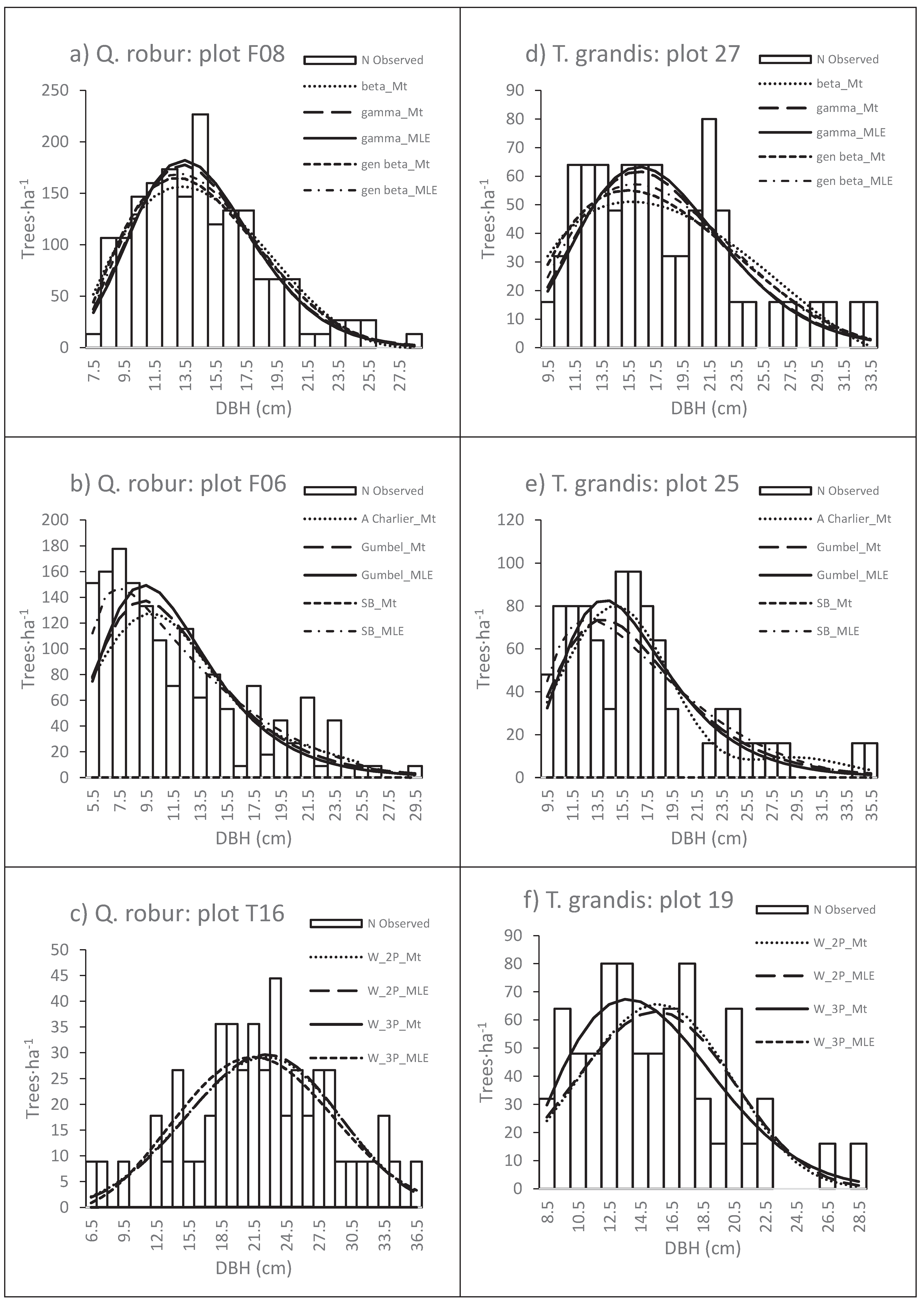
Figure 1 showed a graphical evaluation of the observed and predicted distributions for three even-aged plots each of Q. robur and T. grandis stands. The plots were selected based on high density among the sample plots. The predicted diameter distributions were relatively similar to the observed distributions in both species.
Table 2.
Descriptive statistics of the parameters estimated by derivative (Moments) and numerical optimization (MLE) methods for Quercus robur stands.
Table 2.
Descriptive statistics of the parameters estimated by derivative (Moments) and numerical optimization (MLE) methods for Quercus robur stands.
| Function | Fit | Param | Mean | St Dev | Min | Max |
|---|---|---|---|---|---|---|
| A Charlier |
Derivative (Moments) |
μ | 21.0193 | 5.7681 | 8.3323 | 37.7631 |
| 52.7453 | 32.9372 | 4.0278 | 196.5813 | |||
| Asym | 0.3697 | 0.5164 | -0.9847 | 2.0729 | ||
| Kurt | 0.0548 | 1.017 | -1.1844 | 6.1667 | ||
| beta | Derivative (Moments) |
c | 0.0013 | 0.0030 | 6.00·Exp-11 | 0.0218 |
| L | 6.3530 | 2.5962 | 3.7500 | 19.0125 | ||
| U | 37.9093 | 9.8654 | 16.3000 | 71.6000 | ||
| α | 0.9685 | 0.6740 | -0.1582 | 3.2457 | ||
| γ | 1.3249 | 0.7836 | 0.0083 | 4.4221 | ||
| Gamma-2P | Derivative (Moments) |
α | 10.7038 | 5.5632 | 2.9692 | 29.9842 |
| β | 2.3936 | 1.2093 | 0.4782 | 8.0624 | ||
| Optimization (MLE) |
α | 10.1891 | 5.3742 | 2.9513 | 30.8548 | |
| β | 2.5451 | 1.3837 | 0.4421 | 10.0525 | ||
| generalized beta |
Derivative (Moments) |
170.4135 | 560.1196 | 1.9032 | 4290.0584 | |
| B1 | 6.3530 | 2.5962 | 3.7500 | 19.0125 | ||
| B2 | 37.9093 | 9.8654 | 16.3000 | 71.6000 | ||
| B3 | 1.4699 | 0.9587 | 0.0084 | 4.5858 | ||
| B4 | 2.9449 | 1.4354 | 0.7609 | 7.9256 | ||
| Optimization (MLE) |
209.6410 | 784.4000 | 3.0108 | 7154.8607 | ||
| B1 | 6.3530 | 2.5962 | 3.7500 | 19.0125 | ||
| B2 | 37.9093 | 9.8654 | 16.3000 | 71.6000 | ||
| B3 | 1.5057 | 0.91418 | 0.1710 | 4.0093 | ||
| B4 | 3.0330 | 1.5694 | 0.8589 | 8.4234 | ||
| Gumbel | Derivative (Moments) |
μ | 17.8914 | 5.2504 | 7.4290 | 32.9807 |
| β | 5.4191 | 1.6476 | 1.5648 | 10.9319 | ||
| Optimization (MLE) |
μ | 17.7025 | 5.1462 | 7.4249 | 32.8833 | |
| β | 6.0555 | 1.9661 | 1.5796 | 12.5816 | ||
| Johnson’s SB |
Derivative (Moments) |
ε | 6.3530 | 2.5962 | 3.7500 | 19.0125 |
| λ | 37.9093 | 9.8654 | 16.3000 | 71.6000 | ||
| γ | 0.6328 | 0.3998 | -0.5518 | 1.6197 | ||
| δ | 1.1268 | 0.21093 | 0.7208 | 1.6982 | ||
| Optimization (MLE) |
ε | 6.3530 | 2.5962 | 3.7500 | 19.0125 | |
| λ | 37.9093 | 9.8654 | 16.3000 | 71.6000 | ||
| γ | 0.6296 | 0.3844 | -0.4715 | 1.6283 | ||
| δ | 1.1226 | 0.2021 | 0.7435 | 1.7484 | ||
| Weibull-2P | Derivative (Moments) |
b | 23.3373 | 6.2908 | 9.1039 | 42.2053 |
| c | 3.4887 | 0.9731 | 1.7634 | 6.3410 | ||
| Optimization (MLE) |
b | 23.3570 | 6.2746 | 9.1213 | 42.1990 | |
| c | 3.4653 | 0.9180 | 1.8427 | 6.0898 | ||
| Weibull-3P | Derivative (Moments) |
a | 6.3530 | 2.5962 | 3.7500 | 19.0125 |
| b | 16.4731 | 5.1672 | 5.0848 | 34.7842 | ||
| c | 2.2804 | 0.5399 | 1.3474 | 4.3502 | ||
| Optimization (MLE) |
a | 6.3530 | 2.5962 | 3.7500 | 19.01225 | |
| b | 16.4569 | 5.1075 | 5.0926 | 34.6642 | ||
| c | 2.3116 | 0.54702 | 1.3650 | 4.5155 |
Param: parameter; St Dev: standard deviation; Min: minimum; Max: maximum.
Table 3.
Summary of descriptive statistics of the parameters estimated by derivative (Moments) and numerical optimization (MLE) methods for Tectona grandis stands.
Table 3.
Summary of descriptive statistics of the parameters estimated by derivative (Moments) and numerical optimization (MLE) methods for Tectona grandis stands.
| Function | Fit | Param | Mean | St Dev | Min | Max |
|---|---|---|---|---|---|---|
| A Charlier |
Derivative (Moments) |
μ | 18.6115 | 2.3531 | 13.5467 | 22.8062 |
| 27.5001 | 11.2797 | 12.3188 | 65.1082 | |||
| Asym | 0.57652 | 0.4351 | -0.4617 | 1.4558 | ||
| Kurt | 0.2409 | 1.1994 | -1.1160 | 5.1092 | ||
| beta | Derivative (Moments) |
c | 0.0016 | 0.0039 | 4.95·Exp-11 | 0.0227 |
| L | 7.5775 | 1.6863 | 4.3500 | 11.1750 | ||
| U | 31.7254 | 4.6026 | 21.3000 | 39.2000 | ||
| α | 1.1593 | 0.7226 | 0.1094 | 3.3500 | ||
| γ | 1.6320 | 0.9387 | 0.3156 | 5.1150 | ||
| Gamma-2P | Derivative (Moments) |
α | 14.7649 | 5.6418 | 4.3942 | 28.6115 |
| β | 1.4635 | 0.6380 | 0.6929 | 3.7585 | ||
| Optimization (MLE) |
α | 15.0228 | 5.6265 | 4.3999 | 26.9948 | |
| β | 1.4323 | 0.6207 | 0.7082 | 3.6163 | ||
| Generalized beta |
Derivative (Moments) |
432.0867 | 1194.5728 | 1.9972 | 7589.0738 | |
| B1 | 7.5775 | 1.6863 | 4.3500 | 11.1750 | ||
| B2 | 31.7254 | 4.6026 | 21.3000 | 39.2000 | ||
| B3 | 1.8115 | 0.9587 | 0.0313 | 4.4257 | ||
| B4 | 4.2003 | 1.7369 | 1.0530 | 10.3882 | ||
| Optimization (MLE) |
562.4069 | 1590.6532 | 3.5278 | 11607.4026 | ||
| B1 | 7.5775 | 1.6863 | 4.3500 | 11.1750 | ||
| B2 | 31.7254 | 4.6026 | 21.3000 | 39.2000 | ||
| B3 | 1.9993 | 0.8892 | 0.2448 | 4.1809 | ||
| B4 | 4.5639 | 1.8122 | 1.4330 | 10.8203 | ||
| Gumbel | Derivative (Moments) |
μ | 16.2938 | 2.3630 | 11.4856 | 20.1282 |
| β | 4.0155 | 0.7772 | 2.7366 | 6.2913 | ||
| Optimization (MLE) |
μ | 16.2134 | 2.3629 | 11.3835 | 20.1133 | |
| β | 4.2340 | 0.7465 | 2.7812 | 6.5603 | ||
| Johnson’s SB |
Derivative (Moments) |
ε | 7.5775 | 1.6863 | 4.3500 | 11.1750 |
| λ | 31.7254 | 4.6026 | 21.3000 | 39.2000 | ||
| γ | 0.9011 | 0.3319 | 0.1835 | 1.8047 | ||
| δ | 1.2655 | 0.2212 | 0.7413 | 1.7499 | ||
| Optimization (MLE) |
ε | 7.5775 | 1.6863 | 4.3500 | 11.1750 | |
| λ | 31.7254 | 4.6026 | 21.3000 | 39.2000 | ||
| γ | 0.9090 | 0.3415 | 0.2055 | 1.7963 | ||
| δ | 1.2961 | 0.2090 | 0.8062 | 1.7604 | ||
| Weibull-2P | Derivative (Moments) |
b | 20.4748 | 2.4730 | 15.1130 | 25.0459 |
| c | 4.2068 | 0.9295 | 2.1778 | 6.1998 | ||
| Optimization (MLE) |
b | 20.5079 | 2.4735 | 15.1411 | 25.0836 | |
| c | 3.9932 | 0.8209 | 2.2678 | 6.4435 | ||
| Weibull-3P | Derivative (Moments) |
a | 7.5775 | 1.6863 | 4.3500 | 11.1750 |
| b | 12.4075 | 1.7067 | 8.6744 | 16.6523 | ||
| c | 2.3337 | 0.4648 | 1.3990 | 3.6479 | ||
| Optimization (MLE) |
a | 7.5775 | 1.6863 | 4.3500 | 11.1750 | |
| b | 12.4075 | 1.7067 | 8.6744 | 16.6523 | ||
| c | 2.3337 | 0.4648 | 1.3990 | 3.6479 |
Param: parameter; St Dev: standard deviation; Min: minimum; Max: maximum.
Table 4.
Rank position for each function and statistic for Q. robur and T. grandis stands. Bold texts indicate distributions with the lowest rank sum.
Table 4.
Rank position for each function and statistic for Q. robur and T. grandis stands. Bold texts indicate distributions with the lowest rank sum.
| Species | Fit | Function | Dn | W2 | Bias | MAE | MSE | -ΛΛ | |
| Q. robur | Moments (Derivative) |
A Charlier | 2 | 6 | 7 | 1 | 1 | - | 17 |
| beta | 4 | 8 | 2 | 5 | 5 | - | 24 | ||
| Gamma-2P | 8 | 7 | 6 | 6 | 6 | - | 33 | ||
| Generalized beta | 5 | 3 | 3 | 2 | 3 | - | 16 | ||
| Gumbel | 7 | 5 | 5 | 8 | 8 | - | 33 | ||
| Johnson’s SB | 6 | 1 | 1 | 3 | 2 | - | 13 | ||
| Weibull-2P | 3 | 4 | 8 | 7 | 7 | - | 29 | ||
| Weibull-3P | 1 | 2 | 4 | 4 | 4 | - | 15 | ||
| MLE (Optimization) |
A Charlier | - | - | - | - | - | - | - | |
| beta | - | - | - | - | - | - | - | ||
| Gamma-2P | 6 | 4 | 4 | 4 | 4 | 3 | 25 | ||
| Generalized beta | 4 | 3 | 2 | 3 | 3 | 6 | 21 | ||
| Gumbel | 3 | 6 | 6 | 6 | 6 | 1 | 28 | ||
| Johnson’s SB | 5 | 2 | 1 | 2 | 1 | 5 | 16 | ||
| Weibull-2P | 2 | 5 | 5 | 5 | 5 | 2 | 24 | ||
| Weibull-3P | 1 | 1 | 3 | 1 | 1 | 4 | 11 | ||
| T. grandis | Moments | A Charlier | 3 | 6 | 7 | 3 | 4 | - | 23 |
| (Derivative) | beta | 5 | 8 | 2 | 6 | 6 | - | 27 | |
| Gamma-2P | 7 | 4 | 6 | 5 | 5 | - | 27 | ||
| Generalized beta | 4 | 5 | 3 | 2 | 2 | - | 16 | ||
| Gumbel | 2 | 2 | 4 | 7 | 7 | - | 22 | ||
| Johnson’s SB | 6 | 1 | 1 | 1 | 1 | - | 10 | ||
| Weibull-2P | 8 | 7 | 8 | 8 | 8 | - | 39 | ||
| Weibull-3P | 1 | 3 | 5 | 4 | 2 | - | 15 | ||
| MLE | A Charlier | - | - | - | - | - | - | - | |
| (Optimization) | beta | - | - | - | - | - | - | - | |
| Gamma-2P | 6 | 5 | 4 | 5 | 4 | 3 | 27 | ||
| Generalized beta | 3 | 3 | 2 | 3 | 2 | 5 | 18 | ||
| Gumbel | 2 | 2 | 5 | 4 | 5 | 2 | 20 | ||
| Johnson’s SB | 4 | 1 | 1 | 1 | 1 | 6 | 14 | ||
| Weibull-2P | 5 | 6 | 6 | 6 | 6 | 1 | 30 | ||
| Weibull-3P | 1 | 4 | 3 | 2 | 2 | 4 | 16 |
Figure 1.
Observed and fitted distributions by 8 PDFs to even-aged of Q. robur stands (a, b and c) and T. grandis (d, e and f).
Figure 1.
Observed and fitted distributions by 8 PDFs to even-aged of Q. robur stands (a, b and c) and T. grandis (d, e and f).
4. Discussion
The empirical comparison of eight probability density functions (PDFs) fitted by the derivative and optimization methods for diameter distribution estimation in tropical and Atlantic forests has been evaluated. Among the eight PDFs evaluated for the even-aged Q. robur and T. grandis stands, Johnson’s SB was more consistent in describing the diameter distributions compared to the others. Using either the derivative (moments) and optimization (MLE), Johnson’s SB still provided superior fits than most of the PDFs except Weibull-3P where better fits were observed with optimization in Q. robur. Scolforo et al [42] also found the method of moments and MLE as the preferred fitting methods for Johnson’s SB in describing the diameter distribution in Loblolly pine. Johnson’s SB and Weibull have been used consistently in quantitative forestry studies because of their flexibility to describe different shapes (e.g., [7,14,22,43-45]). Besides the derivative method by moments, the Weibull and Johnson’s SB functions can be fitted by other derivative methods, for example, Weibull by percentiles [46], Johnson’s SB by mode [47], conditional maximum likelihood (CML) [48], linear regression [43], percentiles [49], etc. However, in this study, we used the method of moments because it is the only one that can be used as a derivative method in the eight compared functions.
Gorgoso-Varela et al [7] made a vis-à-vis comparison for each function between several derivative methods and optimization methods. Their results varied depending on the PDF and species. For example, in their study, the generalized beta fitted by derivative and optimization performed better than Johnson’s SB in Gmelina (Gmelina arborea Roxb.) but less so in Tasmanian blue gum (Eucalyptus globulus Labill) and Monterrey pine (Pinus radiata D. Don) stands. Similarly, the generalized beta function fitted with the derivative (moments) was more suitable than Johnson’s SB in describing the diameter distribution of Douglas fir stands [8]. In our study, using the derivative and MLE for the generalized beta yielded good fits but less superior than Johnson’s SB and Weibull 3P function. Few studies have applied the generalized beta function to forestry; rather the beta function by Loetsch et al. [6] has been used consistently particularly, in Mediterranean and Atlantic forests [2,7,14,24]. We found the generalized beta to outperform the beta function in predicting the diameter distribution of Q. robur and T. grandis stands. Compare to the generalized beta, only the derivative method by moments could be used to fit the beta function – making it more conservative than the former. Nevertheless, the beta function was more suitable than the generalized beta for describing the diameter distribution of E. globulus and P. radiata stands in the same region [7].
The A Charlier provided relatively better fits than the beta, Gamma-2P, Weibull-2P and Gumbel functions. This is expected because the A Charlier function is more suitable for even-aged stands, and it is the only function capable of representing bimodal distributions among those evaluated. One limitation of the A Charlier function is that it cannot represent uneven-aged stands that are characterized by a reversed J-shape [17]. In addition, the complex expression of the function may limit its application in practical forestry.
The performance of the 2-parameter PDFs (Gamma-2P, Gumbel and Weibull-2P) was poor and inconsistent in the two species. For example, the Weibull-2P had the best fits in Q. robur stands and worst in T. grandis stands among the 2-parameter functions. On the other hand, the Gumbel that had a similar performance with Gamma-2P in Q. robur, was superior in T. grandis stands. Interestingly, the two-parameter functions had low log-likelihood values (deviance statistic) compared to the higher-level parameter PDFs (Tab. 3). Since this statistic is sensitive to the number of parameters, we recommend that it: should not be used as the only index for comparing distributions; or should be used for comparing distributions with the same number of parameters.
Generally, the Weibull distribution is very flexible, however, imposing a constraint on the location parameter (a = 0) may reduce accuracy and thereby increases its inconsistency in some stands. The Gamma-2P is very inflexible, and as such, may describe negative skewness and model symmetry diameter distribution poorly [49]. It performed poorly in predicting the diameter distribution in mixed natural stands [10] and Nauclea plantation (Nauclea dedirrichii [De Wild.] Merr.) [11] in Nigeria. The Gumbel function is sensitive to extreme values, thus making it suitable for modelling extreme values distribution. Different studies have used the Gumbel function to model the extreme value diameter and/or height distribution with varying degrees of success (e.g., [4,28,29]). Gorgoso-Varela [50] showed that the Gumbel function is a veritable tool that could be used to model the maximum diameter under the green tree retention program.
5. Conclusions
This study has compared the eight probability density functions fitted by derivative and optimization methods used for diameter distribution estimation in Q. robur and T. grandis stands. Johnson’s SB function was more suitable for describing the diameter distribution of the stands. The three-parameter Weibull and generalized beta performed relatively well. Using a numerical method for Johnson’s SB and generalized beta, the frequency of trees in diameter classes could be estimated with ease. If simplicity of function expression were of interest, then three-parameter Weibull could be recommended for the stands. The performances of the functions were consistent irrespective of the fitting methods - derivative or optimization. The fits of the two-parameter functions were generally poor and inconsistent in the Q. robur and T. grandis stands.
Author Contributions
Conceptualization, J.J.G-V; methodology, J.J.G-V and F.N.O.; software, J.J.G-V and F.N.O.; validation, J.J.G-V, S.M.A. and F.N.O.; formal analysis, J.J.G-V and F.N.O.; investigation, J.J.G-V and F.N.O.; resources, J.J.G-V and F.N.O.; data curation, J.J.G-V, S.M.A. and F.N.O.; writing—original draft preparation, J.J.G-V, S.M.A. and F.N.O.; writing—review and editing, J.J.G-V.; visualization, J.J.G-V, S.M.A. and F.N.O.; supervision, J.J.G-V.; project administration, J.J.G-V.; funding acquisition, J.J.G-V. All authors have read and agreed to the published version of the manuscript.
Funding
This research was funded by XUNTA DE GALICIA, grant number PGIDT99MA29101: Estudio epidométrico de las masas de Quercus robur L. en Galicia y su influencia sobre la calidad de la madera.
Data Availability Statement
The data of the research are available contacting with the UXAFORES research group of the University of Santiago de Compostela (Spain).
Conflicts of Interest
The authors declare no conflicts of interest. The funders had no role in the design of the study; in the collection, analyses, or interpretation of data; in the writing of the manuscript; or in the decision to publish the results.
Appendix A
Table A1.
Fits and statistics used in the comparison between Moments and Maximum Likelihood Estimation (MLE) methods for Quercus robur stands.
Table A1.
Fits and statistics used in the comparison between Moments and Maximum Likelihood Estimation (MLE) methods for Quercus robur stands.
| Function | Fit | Dn | W2 | Bias | MAE | MSE | -ΛΛ |
|---|---|---|---|---|---|---|---|
| A Charlier | Moments | 0.1088 | 0.0686 | 0.001370 | 0.018684 | 0.000610 | |
| MLE | No fit | No fit | No fit | No fit | No fit | No fit | |
| beta | Moments | 0.1125 | 0.0705 | 0.000670 | 0.019086 | 0.000632 | |
| MLE | No fit | No fit | No fit | No fit | No fit | No fit | |
| gamma 2P |
Moments | 0.1284 | 0.0692 | 0.001240 | 0.019169 | 0.000648 | |
| MLE | 0.1275 | 0.0663 | 0.001353 | 0.019192 | 0.000649 | -189.76 | |
| Generalized beta |
Moments | 0.1154 | 0.0578 | 0.000897 | 0.018852 | 0.000618 | |
| MLE | 0.1187 | 0.0584 | 0.000913 | 0.019092 | 0.000633 | -175.34 | |
| Gumbel | Moments | 0.1263 | 0.0678 | 0.001229 | 0.019739 | 0.000694 | |
| MLE | 0.1185 | 0.0667 | 0.001746 | 0.019390 | 0.000664 | -190.59 | |
| Johnson’s SB |
Moments | 0.1228 | 0.0435 | 0.000641 | 0.018863 | 0.000617 | |
| MLE | 0.1239 | 0.0523 | 0.000568 | 0.019088 | 0.000627 | -187.85 | |
| Weibull 2P |
Moments | 0.1121 | 0.0650 | 0.001566 | 0.019324 | 0.000659 | |
| MLE | 0.1119 | 0.0661 | 0.001555 | 0.019330 | 0.000660 | -190.50 | |
| Weibull 3P |
Moments | 0.1043 | 0.0489 | 0.001012 | 0.018901 | 0.000623 | |
| MLE | 0.1073 | 0.0513 | 0.000923 | 0.018957 | 0.000627 | -188.51 |
Table A2.
Fits and statistics used in the comparison between Moments and Maximum Likelihood Estimation (MLE) methods for Tectona grandis stands.
Table A2.
Fits and statistics used in the comparison between Moments and Maximum Likelihood Estimation (MLE) methods for Tectona grandis stands.
| Function | Fit | Dn | W2 | Bias | MAE | MSE | -ΛΛ |
|---|---|---|---|---|---|---|---|
| A Charlier | Moments | 0.1273 | 0.0642 | 0.001879 | 0.022755 | 0.000902 | |
| MLE | No fit | No fit | No fit | No fit | No fit | No fit | |
| beta | Moments | 0.1303 | 0.0809 | 0.001456 | 0.023183 | 0.000927 | |
| MLE | No fit | No fit | No fit | No fit | No fit | No fit | |
| gamma 2P |
Moments | 0.1324 | 0.0552 | 0.001797 | 0.023169 | 0.000925 | |
| MLE | 0.1324 | 0.0552 | 0.001706 | 0.023121 | 0.000925 | -142.093 | |
| Generalized beta |
Moments | 0.1285 | 0.0553 | 0.001477 | 0.022736 | 0.000889 | |
| MLE | 0.1270 | 0.0490 | 0.001119 | 0.022851 | 0.000899 | -141.270 | |
| Gumbel | Moments | 0.1239 | 0.0477 | 0.001537 | 0.023632 | 0.000963 | |
| MLE | 0.1239 | 0.0477 | 0.001885 | 0.023033 | 0.000926 | -142.248 | |
| Johnson’s SB |
Moments | 0.1319 | 0.0364 | 0.001100 | 0.022523 | 0.000874 | |
| MLE | 0.1294 | 0.0366 | 0.000878 | 0.022609 | 0.000881 | -140.772 | |
| Weibull 2P |
Moments | 0.1333 | 0.0804 | 0.002460 | 0.024083 | 0.001011 | |
| MLE | 0.1312 | 0.0799 | 0.002793 | 0.024128 | 0.001012 | -144.362 | |
| Weibull 3P |
Moments | 0.1138 | 0.0487 | 0.001575 | 0.022839 | 0.000899 | |
| MLE | 0.1170 | 0.0525 | 0.001575 | 0.022839 | 0.000899 | -141.563 |
References
- Zucchini, W.; Schmidt, M.; Gadow, Kv.. A model for the diameter-height distribution in an uneven-aged beech forest and a method to assess the fit of such models. Silva Fenn. 2001, 35, 169-183.
- Gorgoso-Varela, J.J.; Rojo-Alboreca, A.; Afif-Khouri, E.; Barrio-Anta, M. Modelling diameter distributions of birch (Betula alba L.) and Pedunculate oak (Quercus robur L.) stands in northwest Spain with the beta distribution. Invest. Agrar.: Sist. Recur. For. 2008, 17, 271–281. [Google Scholar] [CrossRef]
- Martin-Benito, D.; Molina-Valero, J.A.; Pérez-Cruzado, C.; Bigler, C.; Bugmann, H. Development and long-term dynamics of old-growth beech-fir forests in the Pyrenees: Evidence from dendroecology and dynamic vegetation modelling. For. Ecol. Manage. 2022, 524, 120541. [Google Scholar] [CrossRef]
- Gorgoso-Varela, J.J.; Rojo-Alboreca, A. Use of Gumbel and Weibull functions to model extreme values of diameter distributions in forest stands. Ann. For. Sci. 2014, 71, 741–750. [Google Scholar] [CrossRef]
- Cao, L.; Zhang, Z.; Yun, T.; Wang, G.; Ruan, H.; She, G. Estimating tree volume distributions in subtropical forests using airborne LiDAR data. Remote Sens. 2019, 11, 97. [Google Scholar] [CrossRef]
- Loetsch, F.; Zöhrer, F.; Haller, K.E. Forest inventory 2. Verlagsgesellschaft, BLV, Munich, Germany, 1973, 469 pp.
- Gorgoso-Varela, J.J.; Ogana, F.N.; Ige, P.O. A comparison between derivative and numerical optimization methods used for diameter distribution estimation. Scand. J. For. Res. 2020, 35, 156–164. [Google Scholar] [CrossRef]
- Li, F.; Zhang, L.; Davis, C.J. Modeling the joint distribution of tree diameters and heights by bivariate generalized Beta distribution. For. Sci. 2002, 48, 47–58. [Google Scholar]
- Podlaski, R. Characterization of diameter distribution data in near-natural forests using the Birnbaum–Saunders distribution. Can. J. For. Res. 2008, 38, 518–527. [Google Scholar] [CrossRef]
- Ogana, F.N.; Osho, J.S.A.; Gorgoso-Varela, J.J. Comparison of beta, gamma and Weibull distributions for characterising tree diameter in Oluwa Forest Reserve, Ondo State, Nigeria. J. Nat. Sci. Res. 2015, 5, 28–36. [Google Scholar]
- Ige, P.O.; Adedapo, S.M. Modelling diameter distributions of Nauclea diderrichii (De Wild.) Merr. stands with Gamma and Weibull functions in Southwest Nigeria. World Scientific News 2021, 160, 247–262. [Google Scholar]
- Fonseca, T.F.; Marques, C.P.; Parresol, B.R. Describing maritime pine diameter distributions with Johnson’s SB distribution using a new all-parameter recovery approach. For Sci. 2009, 55, 367–373. [Google Scholar]
- de Lima, R.A.F.; Batista, J.L.F.; Prado, P.I. Modeling tree diameter distributions in natural forests: an evaluation of 10 statistical models. For. Sci. 2014, 61, 320–327. [Google Scholar] [CrossRef]
- Palahí, M.; Pukkala, T.; Blasco, E.; Trasobares, A. Comparison of beta, Johnson’s SB, Weibull and truncated Weibull functions for modelling the diameter distribution of forest stands in Catalonia (northeast of Spain). Eur. J. Forest Res. 2007, 126, 563–571. [Google Scholar] [CrossRef]
- Arias-Rodil, M.; Diéguez-Aranda, U.; Álvarez-González, J.G.; Pérez-Cruzado, C.; Castedo-Dorado, F.; González-Ferreiro, E. Modeling diameter distributions in radiata pine plantations in Spain with existing countrywide LiDAR data. Ann. For. Sci. 2018, 75, 36. [Google Scholar] [CrossRef]
- Pogoda, P.; Ochał, W.; Orzeł, S. Modeling Diameter Distribution of Black Alder (Alnus glutinosa (L.) Gaertn.) Stands in Poland. Forests 2019, 10, 412. [Google Scholar] [CrossRef]
- Schnur, G.L. Diameter distributions for old-field loblolly pine stands in Maryland. J. Agric. Res. 1934, 49, 731–743. [Google Scholar]
- Cao, Q. Predicting parameters of a Weibull function for modeling diameter distribution. For. Sci. 2004, 50, 682–685. [Google Scholar]
- Mateus, A.; Tomé, M. Modelling the diameter distribution of Eucalyptus plantations with Johnson’s probability density function: parameters recovery from a compatible system of equations to predict stand variables. Ann. For. Sci. 2011, 68, 325–335. [Google Scholar] [CrossRef]
- Sun, S.; Cao, Q.V.; Cao, T. Characterizing diameter distributions for uneven-aged pine-oak mixed forests in the Qinling Mountains of China. Forests 2019, 10, 596. [Google Scholar] [CrossRef]
- Mehtätalo, L.; Lappi, J. Biometry for Forestry and Environmental Data, First ed.; Taylor and Francis, LLC, New York, USA, 2020, 426 pp.
- Zhang, L.; Kevin, C.P.; Chuanmin, L. A comparison of estimation methods for fitting Weibull and Johnson’s SB distributions to mixed spruce-fir stands in north-eastern North America. Can. J. For. Res. 2003, 33, 1340–1347. [Google Scholar] [CrossRef]
- Bončina, Z.; Trifković, V.; Rosset, C.; Klopčič, M. Evaluation of estimation methods for fitting the three-parameter Weibull distribution to European beech forests. iForest 2022, 15, 484. [Google Scholar] [CrossRef]
- Maltamo, M.; Puumalaine, J.; Päivinen, R. Comparison of beta and Weibull functions for modelling basal area diameter distribution in stands of Pinus sylvestris and Picea abies. Scan. J. For. Res. 1995, 10, 284–295. [Google Scholar] [CrossRef]
- Nelson, T.C. Diameter distribution and growth of loblolly pine. Forest Sci. 1964, 10, 105–115. [Google Scholar]
- Gorgoso-Varela, J.J.; Alonso Ponce, R.; Rodríguez-Puerta, F. Modeling Diameter Distributions with Six Probability Density Functions in Pinus halepensis Mill. Plantations Using Low-Density Airborne Laser Scanning Data in Aragón (Northeast Spain). Remote Sens. 2021, 13, 2307. [Google Scholar] [CrossRef]
- Gumbel, E.J. Statistical theory of extreme values and some practical applications. Applied Mathematics Series, 33, Department of Commerce, National Bureau of Standards, Washington, D.C, USA, 1954, 60 pp.
- Gorgoso-Varela, J.J.; García-Villabrille, J.D.; Rojo-Alboreca, A. Modeling extreme values for height distributions in Pinus pinaster, Pinus radiata and Eucalyptus globulus stands in northwestern Spain. iForest 2015, 9, 23–29. [Google Scholar] [CrossRef]
- Ogana, F.N.; Osho, J.S.A.; Gorgoso-Varela, J.J. Application of extreme value distribution for assigning optimum fractions to distribution with boundary parameters: an Eucalyptus plantation case study. Sib. J. For. Sci. 2018, 4, 39–48. [Google Scholar]
- Johnson, N.L. Systems of frequency curves generated by methods of translation. Biometrika 1949, 36, 149–176. [Google Scholar] [CrossRef] [PubMed]
- Cosenza, D.N.; Soares, P.; Guerra-Hernández, J.; Pereira, L.; González-Ferreiro, E.; Castedo-Dorado, F.; Tomé, M. Comparing Johnson’s SB and Weibull Functions to Model the Diameter Distribution of Forest Plantations through ALS data. Remote Sens. 2019, 11, 2792. [Google Scholar] [CrossRef]
- Bailey, R.L.; Dell, T.R. Quantifying Diameter Distributions with the Weibull Function. For. Sci. 1973, 19, 97–104. [Google Scholar]
- Gerald, C.F.; Wheatley, P.O. Applied numerical analysis, 4th ed., Addison-Wesley publishing Co, Reading, Massachusetts, USA, 1989.
- Gorgoso, J.J.; Rojo, A.; Cámara-Obregón, A.; Diéguez-Aranda, U. A comparison of estimation methods for fitting Weibull, Johnson’s SB and beta functions to Pinus pinaster, Pinus radiata and Pinus sylvestris stands in northwest Spain. For. Syst. 2012, 21, 446–459. [Google Scholar] [CrossRef]
- Parresol, B.R. Recovering parameters of Johnson’s SB distribution. US For. Ser. Res. Paper SRS-31. Asheville, USA, 2003, 9 pp. Available online: http://www.treesearch.fs.fed.us/pubs/5455.
- SAS Institute Inc. SAS/STAT 9.1 User’s Guide. Cary, NC, USA, 2004, 5136 pp. 2004.
- R Core Team. R: A language and environment for statistical computing. R Foundation for Statistical Computing, Vienna, Austria. 2021. Available online: https://www.R-project.org/.
- Nelder, J.A.; Mead, R. A simplex algorithm for function minimization. Computer Journal 1965, 7, 308–313. [Google Scholar] [CrossRef]
- Wang, M. Distributional modelling in forestry and remote sensing. PhD thesis, University of Greenwich, London, UK, 2005.
- Wang, M.; Rennolls, K. Bivariate distribution modeling with tree diameter and height data. For. Sci. 2007, 53, 16–24. [Google Scholar]
- Tewari, V.P.; Singh, B. Total wood volume equation for Tectona grandis Linn F. stands in Gujarat, India. J. For. Environ. Sci. 2018, 34, 313–320. [Google Scholar]
- Scolforo, J.R.S.; Vitti, F.C.; Grisi, R.L.; Acerbi, F.; De Assis, A.L. SB distribution’s accuracy to represent the diameter distribution of Pinus taeda, through five fitting methods. For. Ecol. Manage. 2003, 175, 489–496. [Google Scholar] [CrossRef]
- Zhou, B.; McTague, J.P. Comparison and evaluation of five methods of estimation of the Johnson System parameters. Can. J. For. Res. 1996, 26, 928–935. [Google Scholar] [CrossRef]
- Ogana, F.N.; Itam, E.S.; Osho, J.S. Modeling diameter distributions of Gmelina arborea plantation in Omo Forest Reserve, Nigeria with Johnson’s SB. J. Sustain. For. 2017, 36, 121–133. [Google Scholar] [CrossRef]
- Mayrinck, R.C.; Filho, A.C.F.; Ribeiro, A.; de Oliveira, X.M.; de Lima, R.R. A comparison of diameter distribution models for Khaya ivorensis A.Chev. plantations in Brazil. South. For. 2018, 80, 1–8. [Google Scholar] [CrossRef]
- Dubey, S.D. Some percentile estimators for Weibull parameters. Technometrics 1967, 9, 119–129. [Google Scholar] [CrossRef]
- Hafley, W.L.; Buford, M.A. A bivariate model for growth and yield prediction. For. Sci. 1985, 31, 237–247. [Google Scholar]
- Hafley, W.L.; Schreuder, H.T. Statistical distributions for fitting diameter and height data in even-aged stands. Can. J. For. Res. 1977, 7, 481–487. [Google Scholar] [CrossRef]
- Knoebel, B.R.; Burkhart, H.E. A bivariate distribution approach to modeling forest diameter distributions at two points in time. Biometrics 1991, 47, 241–253. [Google Scholar] [CrossRef]
- Gorgoso-Varela, J.J. Species composition and specific aspects of the Green Tree Retention structure in unmanaged mixed forests in Asturias (northern Spain). For. Syst. 2022, 31, e008. [Google Scholar] [CrossRef]
Disclaimer/Publisher’s Note: The statements, opinions and data contained in all publications are solely those of the individual author(s) and contributor(s) and not of MDPI and/or the editor(s). MDPI and/or the editor(s) disclaim responsibility for any injury to people or property resulting from any ideas, methods, instructions or products referred to in the content. |
© 2024 by the authors. Licensee MDPI, Basel, Switzerland. This article is an open access article distributed under the terms and conditions of the Creative Commons Attribution (CC BY) license (http://creativecommons.org/licenses/by/4.0/).
Copyright: This open access article is published under a Creative Commons CC BY 4.0 license, which permit the free download, distribution, and reuse, provided that the author and preprint are cited in any reuse.


