Preprint
Article

Identification of an Open Polynomial Tricompartmental Catenary System of (α+ β) Order by a Linearization Method

Altmetrics

Downloads

102

Views

114

Comments

0

This version is not peer-reviewed

Submitted:

19 January 2024

Posted:

23 January 2024

You are already at the latest version

Alerts
Abstract
To identify the exchange coefficients of a nonlinear polynomial tricompartmental general system of α+β , we follow the procedure; firstly, the recommended solution is to introduce an adequate time t*>0 in a determinable manner. That is, after injecting quantity a into the main compartment, wait a moment for the exchange in the polynomial α+β order nonlinear general system to settle, and then compare this compartment to compartment 2 at t*. Secondly, applying the Taylor formula will linearize the system and identify the exchange coefficients. Finally, we will prove that the linearization method is stable.
Keywords: 
Subject: Biology and Life Sciences  -   Biology and Biotechnology

MSC:  34C35; 3402; 58F40; 9202; 92B05

1. Introduction

Nonlinear compartmental systems of polynomial type are encountered particularly in population dynamics. These systems are controlled by the following hypothesis: "The quantity passing from the compartment i to the compartment j is equal to k i j x i α x j β ( β = 0 if compartment j is outside environment ) where x i ( t ) denotes the mass quantity of compartment i at time t and k i j the exchange coefficient and α , β are constants characterizing the compartmental system. This so-called hypothesis of order polynomial exchange α + β . In the present study our aim is to identify the coefficients exchange of an open polynomial tricompartmental catenary system, using linearization process. The measurements given by the experimenter will be used in conjunction with a time delay technique to adapt the results obtained for identification in linear compartmental systems.

2. Definitions and Notations

We consider the nonlinear tricompartmental system of polynomial type, namely α + β , shown in Figure 1.
The mass balance principle in each compartment leads to nonlinear differential equations (see [2]). The identification is done by exiting the system with and instantaneous injection of substance quantity a in the first compartment. Thus we can say that the tricompartmental catenary system is governed by the following differential system with initial condition:
x 1 ( t ) = k 21 x 2 α ( t ) + k 31 x 3 α ( t ) x 1 β ( t ) k 12 x 2 β ( t ) + k 13 x 3 β ( t ) + k 1 e x 1 α ( t ) x 2 ( t ) = k 12 x 1 α ( t ) + k 32 x 3 α ( t ) x 2 β ( t ) k 21 x 1 β ( t ) + k 23 x 3 β ( t ) x 2 α ( t ) x 3 ( t ) = k 13 x 1 α ( t ) + k 23 x 2 α ( t ) x 3 β ( t ) k 31 x 1 β ( t ) + k 32 x 2 β ( t ) x 3 α ( t ) x 1 ( 0 ) = a x 2 ( 0 ) = 0 x 3 ( 0 ) = 0
we note :
X : 0 , + R 3 t X T ( t ) = x 1 ( t ) , x 2 ( t ) , x 3 ( t )
The state function of the tricompartmental catenary system ( S NL ( P ) ) , is:
F : R 3 R 3 x 1 , x 2 , x 3 F ( x 1 , x 2 , x 3 ) = f 1 ( x 1 , x 2 , x 3 ) , f 2 ( x 1 , x 2 , x 3 ) , f 3 ( x 1 , x 2 , x 3 )
such that:
f 1 ( x 1 , x 2 , x 3 ) = k 21 x 2 α + k 31 x 3 α x 1 β k 12 x 2 β + k 13 x 3 β + k 1 e x 1 α f 2 ( x 1 , x 2 , x 3 ) = k 12 x 1 α + k 32 x 3 α x 2 β k 21 x 1 β + k 23 x 3 β x 2 α f 3 ( x 1 , x 2 , x 3 ) = k 13 x 1 α + k 23 x 2 α x 3 β k 31 x 1 β + k 32 x 2 β x 3 α
With these notations we can write the differential system (1) under the vectorial form:
X T ( X T ( t ) ) X ( 0 ) = a 0 0

3. Preliminary Study

The partial derivatives of the function F being:
f 1 x 1 ( x 1 , x 2 , x 3 ) = β k 21 x 2 α + β k 31 x 3 α x 1 β 1 α k 12 x 2 β + k 13 x 3 β + k 1 e x 1 α 1 f 2 x 1 ( x 1 , x 2 , x 3 ) = α k 12 x 2 β x 1 α 1 β k 21 x 2 α x 1 β 1 f 3 x 1 ( x 1 , x 2 , x 3 ) = α k 13 x 3 β x 1 α 1 β k 31 x 3 α x 1 β 1 ,
f 1 x 2 ( x 1 , x 2 , x 3 ) = α k 21 x 1 β x 2 α 1 β k 12 x 1 α x 2 β 1 f 2 x 2 ( x 1 , x 2 , x 3 ) = β k 12 x 1 α + k 32 x 3 α x 2 β 1 α k 21 x 1 β + k 23 x 3 β x 2 α 1 f 3 x 2 ( x 1 , x 2 , x 3 ) = α k 23 x 3 β x 2 α 1 β k 32 x 3 α x 2 β 1 ,
and
f 1 x 3 ( x 1 , x 2 , x 3 ) = α k 31 x 1 β x 3 α 1 β k 13 x 1 α x 3 β 1 f 2 x 3 ( x 1 , x 2 , x 3 ) = α k 32 x 2 β x 3 α 1 β k 23 x 2 α x 3 β 1 f 3 x 3 ( x 1 , x 2 , x 3 ) = β k 13 x 1 α + k 23 x 2 α x 3 β 1 α k 31 x 1 β + k 32 x 2 β x 3 α 1 .
The function F is differentiable in all point ( x 1 , x 2 , x 3 ) such that x 1 0 , x 2 0 and x 3 0 for all α > 0 and all β > 0 , and the Jacobian matrix is given by:
D F ( x 1 , x 2 , x 3 ) = g 1 ( x 1 , x 2 , x 3 ) α k 1 e x 1 α 1 g 2 ( x 1 , x 2 , x 3 ) 0 g 1 ( x 1 , x 2 , x 3 ) g 2 ( x 1 , x 2 , x 3 ) g 3 ( x 1 , x 2 , x 3 ) g 4 ( x 1 , x 2 , x 3 ) 0 g 3 ( x 1 , x 2 , x 3 ) g 4 ( x 1 , x 2 , x 3 )
with:
g 1 ( x 1 , x 2 , x 3 = α k 12 x 1 α 1 x 2 β β k 21 x 2 α x 1 β 1 g 2 ( x 1 , x 2 , x 3 ) = α k 21 x 2 α 1 x 1 β β k 12 x 1 α x 2 β 1 g 3 ( x 1 , x 2 , x 3 ) = α k 23 x 2 α 1 x 3 β β k 32 x 3 α x 2 β 1 g 4 ( x 1 , x 2 , x 3 ) = α k 32 x 3 α 1 x 2 β β k 23 x 2 α x 3 β 1
For the linearization of the system (2) we apply the Taylor formula in the neighborhood of the initial condition ( a , 0 , 0 ) .
Theorem 3.1. 
1. F is not differentiable in ( a , 0 , 0 ) if α < 0 or β < 0 .
2. 
If α 1 and β 1 F is differentiable in ( a , 0 , 0 ) . The Taylor formula applied in neighborhood of ( a , 0 , 0 ) leads to:
F T ( x 1 , x 2 , x 3 ) = F T ( a , 0 , 0 ) + D F ( a , 0 , 0 ) x 1 a , x 2 , x 3 T + D 2 F ( x θ 1 , x θ 2 , x θ 3 ) x 1 a , x 2 , x 3 2
with: ( x θ 1 , x θ 2 , x θ 3 ) = x 1 + θ x 1 a , x 2 + θ . x 2 , x 3 + θ . x 3 with | θ | < 1 .
For t sufficiently small, we propose to approach the differential system (1) on 0 , t 0 by the following linear differential system:
X T ( a , 0 , 0 ) + D F ( a , 0 , 0 ) x 1 a , x 2 , x 3 T
with
D F ( a , 0 , 0 ) = α k 1 e a α 1 0 0 0 p 21 0 0 0 p 32

3.1. System Delay and Linearization of the System 1

For t > t * > 0 the system S N L ( P ) is then governed by the Cauchy problem:
x 1 ( t ) = k 21 x 2 α ( t ) + k 31 x 3 α ( t ) x 1 β ( t ) k 12 x 2 β ( t ) + k 13 x 3 β ( t ) + k 1 e x 1 α ( t ) x 2 ( t ) = k 12 x 1 α ( t ) x 2 β ( t ) + k 32 x 3 α ( t ) x 2 β ( t ) k 21 x 1 β ( t ) + k 23 x 3 β ( t ) x 2 α ( t ) x 3 ( t ) = k 23 x 2 α ( t ) x 3 β ( t ) k 32 x 3 α ( t ) x 2 β ( t ) x 1 ( t * ) = a * x 2 ( t * ) = b x 3 ( t * ) = c
The Taylor formula on the interval t * , t 0 is given by:
X T a * , b , c + D F ( a * , b , c ) x 1 a * , x 2 b , x 3 c T .
with
D F ( a * , b , c ) = g 1 ( a * , b , c ) α k 1 e a * α 1 g 2 ( a * , b , c ) 0 g 1 ( a * , b , c ) g 2 ( a * , b , c ) g 3 ( a * , b , c ) g 4 ( a * , b , c ) 0 g 3 ( a * , b , c ) g 4 ( a * , b , c )
such that:
g 1 ( a * , b , c ) = α k 12 a * α 1 b β β k 21 b α a * β 1 g 2 ( a * , b , c ) = α k 21 b α 1 a * β β k 12 a * α b β 1 g 3 ( a * , b , c ) = α k 23 c β b α 1 β k 32 b β 1 c α g 4 ( a * , b , c ) = α k 32 b β c α 1 β k 23 c β 1 b α
and
F T ( a * , b , c ) = k 21 b α a * β k 12 a * α b β k 1 e a * α ; k 12 a * α b β + k 32 c α b β k 21 a * β + k 23 c β b α ; k 23 b α c β k 32 c α b β
we pose:
g 1 ( a * , b , c ) = g 1 * g 2 ( a * , b , c ) = g 2 * g 3 ( a * , b , c ) = g 3 * g 4 ( a * , b , c ) = g 4 *
and
f 1 * = k 21 b α a * β k 12 a * α b β k 1 e a * α f 2 * = k 12 a * α b β + k 32 c α b β k 21 a * β + k 23 c β b α f 3 * = k 23 b α c β k 32 c α b β
We can prove that there exists γ , δ and ω such that:
( D F ( ( a * , b , c ) ) ) . γ δ ω = F ( a * , b , c ) .
Indeed
g 1 * g 2 * α k 1 e a * α 1 g 3 * g 5 * g 1 * g 4 * g 3 * g 6 * g 2 * g 4 * g 5 * g 6 * . γ δ ω = f 1 * f 2 * f 3 *
We apply the crammer method: we pose
M = g 1 * g 2 * α k 1 e a * α 1 g 3 * g 5 * g 1 * g 4 * g 3 * g 6 * g 2 * g 4 * g 5 * g 6 * ,
M 1 = f 1 * g 3 * g 5 * f 2 * g 4 * g 3 * g 6 * f 3 * g 4 * g 5 * g 6 * ,
M 2 = g 1 * g 2 * α k 1 e a * α 1 f 1 * g 5 * g 1 * f 2 * g 6 * g 2 * f 3 * g 5 * g 6 * ,
M 3 = g 1 * g 2 * α k 1 e a * α 1 g 3 * f 1 * g 1 * g 4 * g 3 * f 2 * g 2 * g 4 * f 3 * ,
we have d e t M 0 so:
γ = d e t M 1 d e t M δ = d e t M 2 d e t M ω = d e t M 3 d e t M
so we can write the differential system (4) in the equivalent form:
X ( t ) = ( D F ( a * , b , c ) ) . x 1 ( t ) a * + γ x 2 ( t ) b + δ x 3 ( t ) c + ω
therefore:
X ( t ) = ( D F ( a * , b , c ) ) . x 1 ( t ) a * + γ x 2 ( t ) b + δ x 3 ( t ) c + ω
the change of the state function of the tricompartmental system:
Y ( t ) = y 1 ( t ) y 2 ( t ) y 3 ( t ) = x 1 ( t ) a * + γ x 2 ( t ) b + δ x 3 ( t ) c + ω
permits to reduce the system (4) to the canonical form:
Y ( t ) = D F ( a * , d , c ) . Y ( t ) Y T ( t * ) = ( γ * , δ , ω )
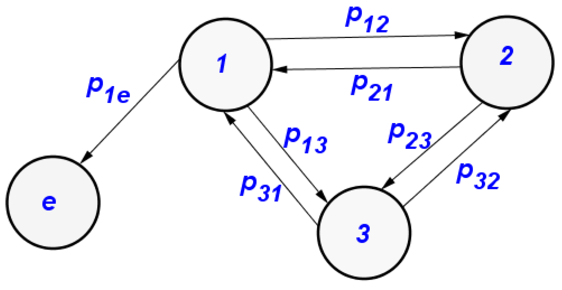
The matrix D F ( a * , b , c ) has the general form of a compartmental matrix, so to this matrix we can associate "formally" the compartmental linear system that we will note S l i n ( T P ) represented by the following figure:
with:
p 12 = α k 12 a * α 1 b β β k 21 b α a * β 1 p 13 = α k 13 c β a * α 1 β k 31 a * β 1 c α p 21 = α k 21 b α 1 a * β β k 12 a * α b β 1 p 23 = α k 23 c β b α 1 β k 32 b β 1 c α p 31 = α k 31 a * β c α 1 β k 13 c β 1 a * α p 32 = α k 32 b β c α 1 β k 23 c β 1 b α p 1 e = α k 1 e a * α 1
Proposition 1. 
The real numbers a * , b and c such that the exchange coefficients p i j / i , j = 1 , 2 , 3 i j is strictly than zero if and only if α > β > 1 .
exist if and only if α > β > 1 .
Proof. 
Knowing that:
p 12 > 0 p 21 > 0 α k 12 a * α β k 21 b α β a * β > 0 α k 21 b α β a * β β k 12 a * α > 0
and
p 23 > 0 p 32 > 0 α k 23 b α β k 32 b β c α β > 0 α k 32 b β c α β β k 23 b α > 0
and
p 13 > 0 p 31 > 0 α k 13 a * α β k 31 a * β c α β > 0 α k 31 c α β a * β β k 13 a * α > 0
we pose:
x = k 12 a * α x = k 23 b α x = k 13 a * α and y = k 21 b α β a * β y = k 32 b β c α β y = k 31 a * β c α β
then
p 12 > 0 p 21 > 0 α x β y > 0 ( S ) α y β x > 0
p 23 > 0 p 32 > 0 α x β y > 0 ( S ) α y β x > 0
p 13 > 0 p 31 > 0 α x β y > 0 ( S ) α y β x > 0
then
if α β the set of solutions of the systems ( S ) ; ( S ) and ( S ) is empty .
if α > β > 1 the set of solutions of the systems ( S ) ; ( S ) and ( S ) is not empty. □

4. Calculation of the Exchange Coefficients p i j / i , j = 1 , 2 , 3 i j of the System S l i n ( T P ) and the Excretion Coefficient p 1 e

Note the compartmental matrix of the linear model S l i n ( T P ) by:
A = p 12 p 13 p 1 e p 21 p 31 p 12 p 21 p 23 p 32 p 13 p 23 p 32 p 31
The matrix A being tridiagonal and compartmental, its eigenvalues noted λ i i 1 , 2 , 3 are real, distinct and strictly negative. The general solution of the system is written in the form
y j ( t ) = i = 1 3 β i j e x p λ i t i 1 , 2 , 3
where β i j i 1 , 2 , 3 is the j th column of the matrix B of the elementary masses, associated with the i compartment. The measurements made on the first and the second compartment make the minimization of the functional J introduced by Y.Cherruault [4] possible:
J β k i , λ k , 1 i 2 , 1 k 3 = j = 1 m i = 1 2 x i ( t j ) k = 1 3 β k i e λ k t j 2
we put:
min J β k i , λ k , 1 i 2 , 1 k 3 = J β k i * , λ k * , 1 i 2 , 1 k 3
the functions φ i , i 1 , 2 , 3 defined by:
φ i t = exp λ i * t , t t * , i 1 , 2 , 3
being linearly independent we can conclude that for every integer i in 1 , 2 , 3 we have:The matrix A being tridiagonal and compartmental, its eigenvalues noted λ i i 1 , 2 , 3 are real, distinct and strictly negative. The general solution of the system is written in the form
y j ( t ) = i = 1 n β i j e x p λ i t i 1 , 2 , 3
where β i j i 1 , 2 , 3 is the j th column of the matrix B of the elementary masses, associated with the i compartment. The measurements made on the first and the second compartment make the minimization of the functional J introduced by Y.Cherruault [4] possible:
J β k i , λ k , 1 i 2 , 1 k 3 = j = 1 m i = 1 2 x i ( t j ) k = 1 3 β k i e λ k t j 2
we put:
min J β k i , λ k , 1 i 2 , 1 k 3 = J β k i * , λ k * , 1 i 2 , 1 k 3
the functions φ i , i 1 , 2 , 3 defined by:
φ i t = exp λ i * t , t t * , i 1 , 2 , 3
being linearly independent we can conclude that for every integer i in 1 , 2 , 3 we have:
λ i * β i 1 * = p 12 p 13 p 1 e β i 1 * + p 21 β i 2 * + p 31 β i 3
λ i * β i 2 * = p 12 β i 1 * p 21 p 23 β i 2 * + p 32 β i 3
λ i * β i 3 = p 13 β i 1 * + p 23 β i 2 * p 31 + p 32 β i 3

4.1. Calculating of Excretion Coefficient p 1 e

We have a relationship (1) for all t 0 :
x 1 ( t ) + x 2 ( t ) + x 3 ( t ) = k 1 e x 1 α ( t )
for t = t * and t = t 0 such as t * t 0 0 we have:
x 1 ( t * ) + x 2 ( t * ) + x 3 ( t * ) = k 1 e x 1 α ( t * )
x 1 ( t 0 ) + x 2 ( t 0 ) + x 3 ( t 0 ) = k 1 e x 1 α ( t 0 )
therefore:
x 1 ( t * ) + x 2 ( t * ) + x 3 ( t * ) x 1 ( t 0 ) + x 2 ( t 0 ) + x 3 ( t 0 ) = x 1 α ( t * ) x 1 α ( t 0 )
so:
x 1 ( t * ) + x 2 ( t * ) x 1 α ( t 0 ) + x 3 ( t * ) x 1 α ( t 0 ) = x 1 ( t 0 ) + x 2 ( t 0 ) x 1 α ( t * ) + x 3 ( t 0 ) x 1 α ( t * )
so:
x 3 ( t * ) x 1 α ( t 0 ) x 3 ( t 0 ) x 1 α ( t * ) = x 1 ( t 0 ) + x 2 ( t 0 ) x 1 ( t * ) + x 2 ( t * ) ξ
the relation (12) which is equivalent to:
x 1 ( t * ) + x 2 ( t * ) x 1 α ( t 0 ) + x 3 ( t * ) x 1 α ( t 0 ) = k 1 e x 1 α ( t * ) x 1 α ( t 0 )
and the relation (13) which is equivalent to:
x 1 ( t 0 ) + x 2 ( t 0 ) x 1 α ( t * ) + x 3 ( t 0 ) x 1 α ( t * ) = k 1 e x 1 α ( t 0 ) x 1 α ( t * )
therefore:
x 1 ( t * ) + x 2 ( t * ) x 1 α ( t 0 ) x 1 ( t 0 ) + x 2 ( t 0 ) x 1 α ( t * ) + ξ = k 1 e x 1 α ( t 0 ) x 1 α ( t * ) x 1 α ( t * ) x 1 α ( t 0 )
then
k 1 e = x 1 ( t * ) + x 2 ( t * ) x 1 α ( t 0 ) x 1 ( t 0 ) + x 2 ( t 0 ) x 1 α ( t * ) + ξ x 1 α ( t 0 ) x 1 α ( t * ) x 1 α ( t * ) x 1 α ( t 0 )
and we have
p 1 e = α k 1 e a * α 1
Theorem 4.1. 
adding the equations (9), (10) and (11) we get:
β i 3 = β i 1 * β i 2 * p 1 e β i 1 * λ i * i 1 ; 2 ; 3

4.2. Calculating the Exchange Coefficients p i j / i , j = 1 , 2 , 3 i j

The relation (9) allows to write:
λ 1 * β 1 1 * = p 12 p 13 p 1 e β 1 1 * + p 21 β 1 2 * + p 31 β 1 3 *
λ 2 * β 2 1 * = p 12 p 13 p 1 e β 2 1 * + p 21 β 2 2 * + p 31 β 2 3 *
λ 3 * β 3 1 * = p 12 p 13 p 1 e β 3 1 * + p 21 β 3 2 * + p 31 β 3 3 *
by multiplying both sides of the relation (18) by the number β 2 1 * and the relation (19) by the number β 1 1 * and by adding the two relations side by side, we obtain
λ 1 * λ 2 * β 1 1 * β 2 1 * = p 21 β 1 2 * β 2 1 * β 2 2 * β 1 1 * + p 31 β 1 3 * β 2 1 * β 1 1 * β 2 3 *
and by multiplying both sides of the relation (19) by the number β 3 1 * and the relation (20) by the number β 2 1 * and by adding the two relations side by side, we obtain
λ 2 * λ 3 * β 2 1 * β 3 1 * = p 21 β 2 2 * β 3 1 * β 3 2 * β 2 1 * + p 31 β 2 3 * β 3 1 * β 3 3 * β 2 1 *
which is equivalent to:
λ 1 * λ 2 * β 1 1 * β 2 1 * λ 2 * λ 3 * β 2 1 * β 3 1 * = β 1 2 * β 2 1 * β 2 2 * β 1 1 * β 1 3 * β 2 1 * β 1 1 * β 2 3 * β 2 2 * β 3 1 * β 3 2 * β 2 1 * β 2 3 * β 3 1 * β 3 3 * β 2 1 * p 21 p 31
K
if d e t K 0 then
p 21 = d e t K 1 d e t K p 31 = d e t K 2 d e t K
such as
K 1 = λ 1 * λ 2 * β 1 1 * β 2 1 * β 1 3 * β 2 1 * β 1 1 * β 2 3 * λ 2 * λ 3 * β 2 1 * β 3 1 * β 2 3 * β 3 1 * β 3 3 * β 2 1 * K 2 = β 1 2 * β 2 1 * β 2 2 * β 1 1 * λ 1 * λ 2 * β 1 1 * β 2 1 * β 2 2 * β 3 1 * β 3 2 * β 2 1 * λ 2 * λ 3 * β 2 1 * β 3 1 *
and the relation (10) allows to write:
λ 1 * β 1 2 * = p 12 β 1 1 * p 21 p 23 β 1 2 * + p 32 β 1 3 *
λ 2 * β 2 2 * = p 12 β 2 1 * p 21 p 23 β 2 2 * + p 32 β 2 3 *
λ 3 * β 3 2 * = p 12 β 3 1 * p 21 p 23 β 3 2 * + p 32 β 3 3 *
by multiplying both sides of the relation (26) by the number β 2 2 * and the relation (27) by the number β 1 2 * and by adding the two relations side by side, we obtain
λ 1 * λ 2 * β 1 2 * β 2 2 = p 12 β 1 * β 2 2 * β 2 1 * β 1 2 * + p 32 β 1 3 * β 2 2 * β 1 2 * β 2 3 *
by multiplying both sides of the relation (27) by the number β 3 2 * and the relation (28) by the number β 2 2 * and by adding the two relations side by side, we obtain
λ 2 * λ 3 * β 2 2 * β 3 2 * = p 12 β 2 1 * β 3 2 * β 3 1 * β 2 2 * + p 32 β 2 3 * β 3 2 * β 3 3 * β 2 2 *
so
λ 1 * λ 2 * β 1 2 * β 2 2 λ 2 * λ 3 * β 2 2 * β 3 2 * = β 1 * β 2 2 * β 2 1 * β 1 2 * β 1 3 * β 2 2 * β 1 2 * β 2 3 * β 2 1 * β 3 2 * β 3 1 * β 2 2 * β 2 3 * β 3 2 * β 3 3 * β 2 2 * p 12 p 32 K
if d e t K 0 then
p 12 = d e t K 1 d e t K p 32 = d e t K 2 d e t K
such as
K 1 = λ 1 * λ 2 * β 1 2 * β 2 2 β 1 3 * β 2 2 * β 1 2 * β 2 3 * λ 2 * λ 3 * β 2 2 * β 3 2 * β 2 3 * β 3 2 * β 3 3 * β 2 2 *
and
K 2 = β 1 * β 2 2 * β 2 1 * β 1 2 * λ 1 * λ 2 * β 1 2 * β 2 2 β 2 1 * β 3 2 * β 3 1 * β 2 2 * λ 2 * λ 3 * β 2 2 * β 3 2 *
and the relation (11) allows to write:
λ 1 * β 1 3 * = p 13 β 1 1 * + p 23 β 1 2 * p 31 + p 32 β 1 3 *
λ 2 * β 2 3 * = p 13 β 2 1 * + p 23 β 2 2 * p 31 + p 32 β 2 3 *
λ 3 * β 3 3 * = p 13 β 3 1 * + p 23 β 3 2 * p 31 + p 32 β 3 3 *
by multiplying both sides of the relation (31) by the number β 2 3 * and the relation (32) by the number β 1 3 * and by adding the two relations side by side, we obtain
λ 1 * λ 2 * β 1 3 * β 2 3 * = p 13 β 1 1 * β 2 2 * β 2 1 * β 1 3 * + p 23 β 1 2 * β 2 3 * β 2 2 * β 2 3 *
and by multiplying both sides of the relation (32) by the number β 3 3 * and the relation (33) by the number β 2 3 * and by adding the two relations side by side, we obtain
λ 2 * λ 3 * β 2 3 * β 3 3 * = p 13 β 2 1 * β 3 3 * β 3 1 β 2 3 * + p 23 β 2 2 * β 3 3 * β 3 2 * β 2 3 *
so
λ 1 * λ 2 * β 1 3 * β 2 3 * λ 2 * λ 3 * β 2 3 * β 3 3 * = β 1 1 * β 2 2 * β 2 1 * β 1 3 * β 1 2 * β 2 3 * β 2 2 * β 2 3 * β 2 1 * β 3 3 * β 3 1 β 2 3 * β 2 2 * β 3 3 * β 3 2 * β 2 3 * p 13 p 32 K
if d e t K 0 then
p 13 = d e t K 1 d e t K p 23 = d e t K 2 d e t K
such as
K 1 = λ 1 * λ 2 * β 1 3 * β 2 3 * β 1 2 * β 2 3 * β 2 2 * β 2 3 * λ 2 * λ 3 * β 2 3 * β 3 3 * β 2 2 * β 3 3 * β 3 2 * β 2 3 *
and
K 2 = β 1 1 * β 2 2 * β 2 1 * β 1 3 * λ 1 * λ 2 * β 1 3 * β 2 3 * β 2 1 * β 3 3 * β 3 1 β 2 3 * λ 2 * λ 3 * β 2 3 * β 3 3 *
Let’s put:
p 1 e = η 1 * p 12 = η 2 * p 21 = η 3 * p 23 = η 4 * p 32 = η 5 * p 13 = η 6 * p 31 = η 7 *

4.3. Calculating the Initial Condition c

The initial condition c is determined by:
c = η 7 * + η 5 * 1 α + β λ 1 * β 1 3 * e λ 1 * t * + λ 2 * β 2 3 * e λ 2 * t * + λ 3 * β 3 3 * e λ 3 * t * + a * η 6 * + b η 4 *
Proof. 
We have
x 3 ( t * ) = k 13 a * α c β + k 23 b α c β k 31 c α b β + k 32 c α a * β
and we have
y 3 ( t * ) = λ 1 * β 1 3 * e λ 1 * + λ 2 * β 2 3 * e λ 2 * t * + λ 3 * β 2 3 * e λ 3 * t *
and consequently
k 13 a * α c β + k 23 b α c β k 31 c α b β + k 32 c α a * β = λ 1 * β 1 3 * e λ 1 * + λ 2 * β 2 3 * e λ 2 * t * + λ 3 * β 2 3 * e λ 3 * t *
furthermore we have:
η 4 * = α k 23 c β b α 1 β k 32 b β 1 c α η 5 * = α k 32 b β c α 1 β k 23 c β 1 b α η 6 * = α k 13 c β a * α 1 β k 31 a * β 1 c α η 7 * = α k 31 a * β c α 1 β k 13 c β 1 a * α
which equivalent:
b e t a 4 * = α k 23 c β b α β k 32 b β c α c η 5 * = α k 32 b β c α β k 23 c β b α a * η 6 * = α k 13 c β a * α β k 31 a * β c α c η 7 * = α k 31 a * β c α β k 13 c β a * α
and consequently:
b η 4 * c η 5 * = α + β k 23 c β b α k 32 c α b β a * η 6 * c η 7 * = α + β k 13 c β a * α k 31 a * β c α
which implies:
b η 4 * + a * η 6 * c η 7 * + η 5 * = α + β k 23 c β b α + k 13 c β a * α k 31 a * β c α + k 32 c α b β
so
c = η 7 * + η 5 * 1 α + β k 31 a * β c α + k 32 c α b β k 23 c β b α + k 13 c β a * α + b η 4 * + a * η 6 * y 3 ( t * )
finally, we get:
c = η 7 * + η 5 * 1 α + β λ 1 * β 1 3 * e λ 1 * t * + λ 2 * β 2 3 * e λ 2 * t * + λ 3 * β 3 3 * e λ 3 * t * + a * η 6 * + b η 4 *

4.4. Calculating the Exchange Coefficients k i j i , j = 1 , 2 , 3

Proposition 2. 
Let p * = β 1 1 * β 1 2 * β 1 3 * β 2 1 * β 2 2 * β 2 3 * β 3 1 * β 3 2 * β 3 3 * the associated partial matrix of measures to the system S l i n ( p ) identified by (6) if α > β > 1 then the system nonlinear S N L ( p ) is additionally identified
k 1 e   has already calculated
and
k 12 = d e t Q 1 d e t Q k 21 = d e t Q 2 d e t Q k 13 = d e t Q 1 d e t Q k 31 = d e t Q 2 d e t Q k 23 = d e t Q 1 d e t Q k 21 = d e t Q 2 d e t Q
such as
Q = α a * α 1 b β β b α a * β 1 β a * α b β 1 α a * β b * α 1 Q 1 = η 2 * β b α a * β 1 η 3 * α a * β b * α 1 Q = α a * α 1 b β η 2 * β a * α b β 1 η 3 *
Q = α c β a * α 1 β a * β 1 c α β c β 1 a * α α a * β c α 1 Q 1 = η 6 * β a * β 1 c α η 7 * α a * β c α 1 Q 2 = α c β a * α 1 η 6 * β c β 1 a * α η 7 *
Q = α c β b α 1 β b β 1 c α β c β 1 b α α b β c α 1 Q 1 = η 4 * β b β 1 c α η 5 * α b β c α 1 Q 2 = α c β b α 1 η 4 * β c β 1 b α η 5 *
Proof. 
We have α > β which implies that d e t Q , d e t Q and d e t Q do not equal zero and we have
η 2 * = α k 12 a * α 1 b β β k 21 b α a * β 1 η 3 * = α k 21 b α 1 a * β β k 12 a * α b β 1 η 4 * = α k 23 c β b α 1 β k 32 b β 1 c α η 5 * = α k 32 b β c α 1 β k 23 c β 1 b α η 6 * = α k 13 c β a * α 1 β k 31 a * β 1 c α η 7 * = α k 31 a * β c α 1 β k 13 c β 1 a * α
we apply Crammer’s method, we easily find the solutions □

5. Stability of the Linearization Method

For all i , j = 1 ; 2 ; 3 w i t h j > i we set p ¯ i j = ϑ i j * and p ¯ j i = ϑ j i * such that p ¯ i j i , j = 1 ; 2 ; 3 i j the exchange coefficients of a real linear compartmental system and note that the exchange coefficients of a real nonlinear compartmental system by k ¯ i j i , j = 1 ; 2 ; 3
And note that ε i j the errors made on the calculation of p i j i ; j = 1 ; 2 ; 3 j > i and ε j i the errors made on the calculation of p j i i ; j = 1 ; 2 ; 3 j > i
and we set a * = ξ 1 , b = ξ 2 and c = ξ 3 .
Proposition 3. 
We can approximate the exchange coefficients of nonlinear polynomial system by:
k ¯ i j = α ξ i ϑ i * + β ξ j ϑ j * ( α 2 β 2 ) ξ j β ξ i α k ¯ j i = β ξ i ϑ i * + ξ j α ϑ j * ( α 2 β 2 ) ξ j α ξ i β
which represent the respective approximations of the exchange coefficients k i j i , j = 1 , 2 , 3 ; i j
| k i j k ¯ i j | α ξ i + ξ j β m a x ε i j , ε j i ( α 2 β 2 ) ξ j β ξ i α | k j i k ¯ j i | β ξ i + ξ j α m a x ε i j , ε j i ( α 2 β 2 ) ξ j α ξ i β
Proof. 
ϑ i j * being an approximation of p i j then there is ε i j ( | ε i j | ε i j ) such that:
ϑ i * + ε i j = α k i j ξ j β ξ i α 1 β k j i ξ j α ξ i β 1
and consequently:
α ξ j 1 ξ i ( ϑ i * + ε i j ) = α 2 k i j ξ j β 1 ξ i α α β k j i ξ j α 1 ξ i β
Proposition 4. 
ϑ j * being an approximation of p j i then there exists ε j i ( | ε j i | ε j i ) such that:
ϑ j * + ε j i = α k j i ξ j α 1 ξ i β β k i j ξ j β 1 ξ i α
and consequently
β ( ϑ j * + ε j i ) = α β k j i ξ j α 1 ξ i β β 2 k i j ξ j β 1 ξ i α
by adding the two relations (39) and (41) side by side, we obtain
α ξ j 1 ξ i ( ϑ i * + ε i j ) + β ( ϑ j * + ε j i ) = α 2 k i j ξ j β 1 ξ i α β 2 k i j ξ j β 1 ξ i α
Which is equivalent to:
α ξ i ( ϑ i * + ε i j ) + β ξ j ( ϑ j * + ε j i ) = k i j ( α 2 β 2 ) ξ j β ξ i α
so
k i j = α ξ i ( ϑ i * + ε i j ) + β ξ j ( ϑ j * + ε j i ) ( α 2 β 2 ) ξ j β ξ i α
the relation (38) which is equivalent to:
β ξ i ξ j 1 ( ϑ i * + ε i j ) = β α k i j ξ j β 1 ξ i α β 2 k j i ξ j α 1 ξ i β
the relation (40) which is equivalent to:
α ( ϑ j * + ε j i ) = α 2 k j i ξ j α 1 ξ i β β α k i j ξ j β 1 ξ i α
and by adding the two relations (42) and (43) side by side, we obtain
β ξ i ξ j 1 ( ϑ i * + ε i j ) + α ( ϑ j * + ε j i ) = α 2 k j i ξ j α 1 ξ i β β 2 k j i ξ j α 1 ξ i β
which is equivalent to:
β ξ i ( ϑ i * + ε i j ) + ξ j α ( ϑ j * + ε j i ) = α 2 k j i ξ j α ξ i β β 2 k j i ξ j α ξ i β = k j i ( α 2 β 2 ) ξ j α ξ i β
as a result
k j i = β ξ i ( ϑ i * + ε i j ) + ξ j α ( ϑ j * + ε j i ) ( α 2 β 2 ) ξ j α ξ i β
so
k ¯ i j = lim ( ε i j , ε j i ) ( 0 , 0 ) α ξ i ( ϑ i * + ε i j ) + β ξ j ( ϑ j * + ε j i ) ( α 2 β 2 ) ξ j β ξ i α = α ξ i ϑ i * + β ξ j ϑ j * ( α 2 β 2 ) ξ j β ξ i α .
Proposition 5. 
k ¯ j i = lim ( ε i j , ε j i ) ( 0 , 0 ) β ξ i ( ϑ i * + ε i j ) + ξ j α ( ϑ j * + ε j i ) ( α 2 β 2 ) ξ j α ξ i β = β ξ i ϑ i * + ξ j α ϑ j * ( α 2 β 2 ) ξ j α ξ i β
therefore
| k i j k ¯ i j | = α ξ i ( ϑ i * + ε i j ) + β ξ j ( ϑ j * + ε j i ) ( α 2 β 2 ) ξ j β ξ i α α ξ i ϑ i * + ξ j β ϑ j * ( α 2 β 2 ) ξ j β ξ i α
= α ξ i ε i j + ξ j β ε j i ( α 2 β 2 ) ξ j β ξ i α α ξ i + ξ j β m a x ε i j , ε j i ( α 2 β 2 ) ξ j β ξ i α
α ξ i + ξ j β m a x ε i j , ε j i ( α 2 β 2 ) ξ j β ξ i α
and
| k j i k ¯ j i | = β ξ i ( ϑ i * + ε i j ) + α ξ j ( ϑ j * + ε j i ) ( α 2 β 2 ) ξ j α ξ i β β ξ i ϑ i * + ξ j α ϑ j * ( α 2 β 2 ) ξ j α ξ i β
= β ξ i ε i j + ξ j α ε j i ( α 2 β 2 ) ξ j α ξ i β β ξ i + ξ j α m a x ε i j , ε i i ( α 2 β 2 ) ξ j α ξ i β
β ξ i + ξ j α m a x ε i j , ε j i ( α 2 β 2 ) ξ j α ξ i β
Theorem 5.1. 
see [7] We have:
p 1 e = p ¯ 1 e
so
k 1 e = p ¯ 1 e α a * α 1 .
Conclusion 6. 
The linear model associated to the non linear polynomial tricompartmental general system of ( α + β ) order involves four important difficulties:
1. 
The initial condition at time t = 0 does not permit to give a complete information about the model ( S NL ( P ) ) . A temporization t * is introduced to suppress this difficulty.
2. 
If this temporization is not modulated, the linear model is not necessarily real. We have shown that the measures done on the compartment 1 and on the compartment 2 permit to choose one measure at instant t i 1 = t * such that we can develop a linearization method.
3. 
The nonhomogeneous condition x 3 ( t * ) = c being unknown is identified form measures done on compartment 1 and on compartment 2.
4. 
The linearization method is stable.

Author Contributions

All authors contributed equally to this work.

Funding

No funding applied in this work.

Data Availability Statement

All data generated or analyzed during this study are included in this published article.

Acknowledgments

The authors would like to thank the anonymous referees and the handling editor for their reading and relevant remarks/suggestions.

Conflicts of Interest

The authors declare no conflicts of interest.

References

  1. Cherruault, Y. Biomathématiques, Collection “Que sais-jeâ€. Presses Universitaires de France, (P.U.F), Paris, 1983, no 2052.
  2. Cherruault, Y. Modèles et méthodes mathématiques pour les sciences, du vivant; Presses Universitaires de France, (P.U.F) Paris; 1999.
  3. Cherruault, Y. Optimisation: Méthodes locales et globales; Presses Universitaires De France; 1999.
  4. Hebri, B., and Cherruault, Y. Direct identification of general linear compartmental systems by means of n − 2 compartments measures. Kybernetes 2005, 34.7/8, 969–982. [CrossRef]
  5. Hebri, B., and Cherruault, Y. Identification of a nonlinear polynomial compartmental system of α + β order by a linearization method. Mathematical Modelling and Analysis 2006, 11.2, 149–160.
  6. Hebri, B., and Cherruault, Y. New results about the identifiability of linear open bicompartmental homogeneous system and the identification of open Michaelis-Menten system by a linear approach. Kybernetes2005, 34.7/8, 1159–1186. [CrossRef]
  7. Hebri, B. Khelifa, S., and Cherruault, Y. Stability of the linearization method in compartmental analysis.Kybernetes 2009, 38.5, 744–761. [CrossRef]
  8. Schwartz, L. Etude de sommes d’exponentielles; Hermann; Paris; 1959.
  9. Sibony, M., and Mardon, J.Cl. Analyse numérique I; Hermann; 1982.
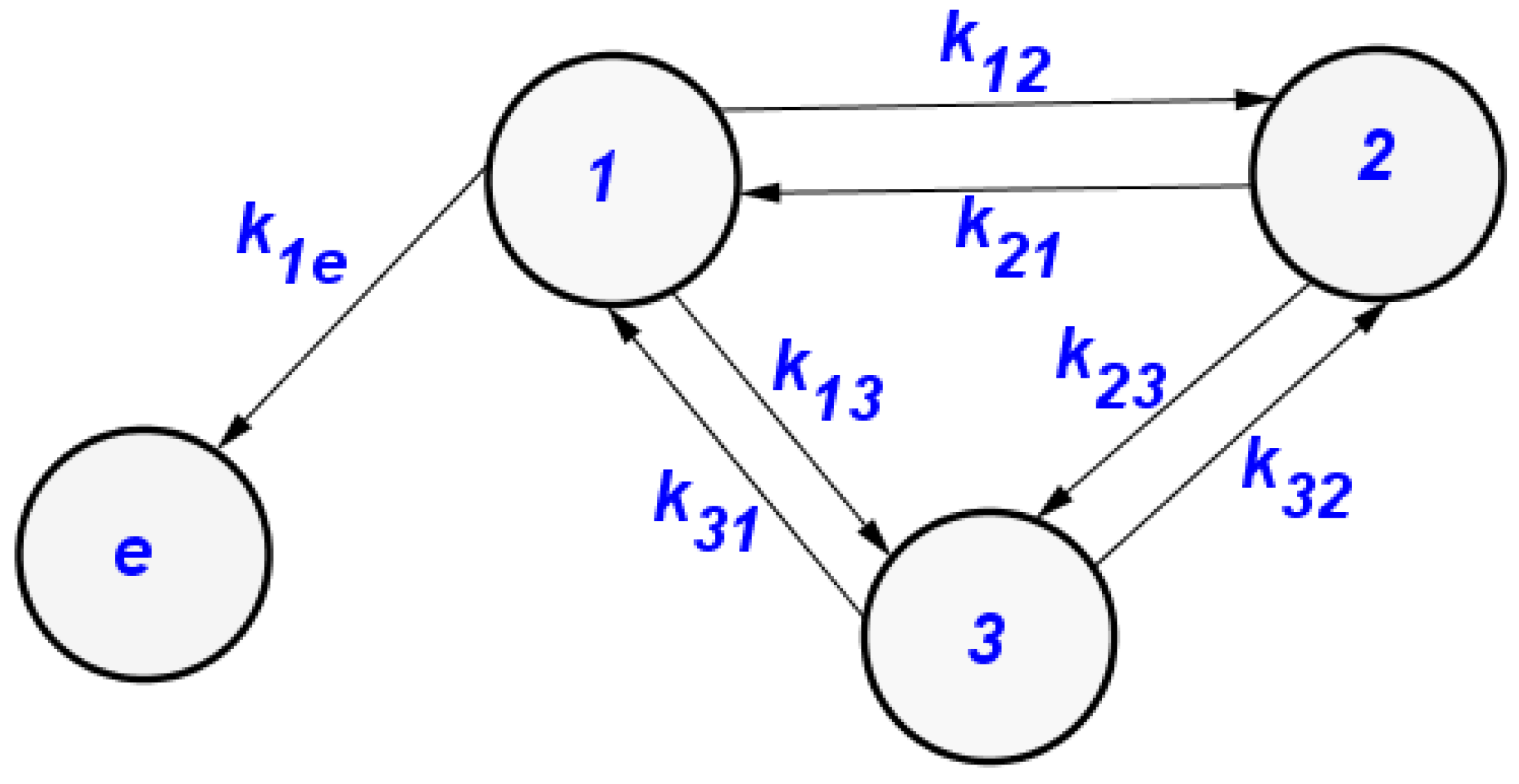
Figure 1. S N L ( P ) :Nonlinear polynomial tricompartmental system
Preprints 96890 g001
Figure 2. S L ( P ) :Linear Polynomial tricompartment System
Preprints 96890 g002
Disclaimer/Publisher’s Note: The statements, opinions and data contained in all publications are solely those of the individual author(s) and contributor(s) and not of MDPI and/or the editor(s). MDPI and/or the editor(s) disclaim responsibility for any injury to people or property resulting from any ideas, methods, instructions or products referred to in the content.
Copyright: This open access article is published under a Creative Commons CC BY 4.0 license, which permit the free download, distribution, and reuse, provided that the author and preprint are cited in any reuse.
Prerpints.org logo

Preprints.org is a free preprint server supported by MDPI in Basel, Switzerland.

Subscribe

© 2024 MDPI (Basel, Switzerland) unless otherwise stated