Effect of the root parameter on the stability of the Non-stationary D/M/1 queue’s GI/M/1 model with PSFFA applications to the Internet of Things (IoT)

Preprint

Article

Effect of the root parameter on the stability of the Non-stationary D/M/1 queue’s GI/M/1 model with PSFFA applications to the Internet of Things (IoT)

Altmetrics

Downloads

Views

Comments

Dr Ismail A Mageed^*

This version is not peer-reviewed

This preprints belongs to the Topic

Future Internet Architecture: Difficulties and Opportunities

Submitted:

24 January 2024

Posted:

26 January 2024

You are already at the latest version

Alerts

Abstract

An exposition is undertaken to reveal the significant impact of the time-dependent root parameter, on the stability of Pointwise Stationary Fluid Flow Approximation (PSFFA) model of the non-stationary queueing system. This opens new grounds to stability analysis of non-stationary queueing systems. Potential PSFFA applications of IoT are highlighted.

Keywords:

Subject: Computer Science and Mathematics - Probability and Statistics

1. Introduction

Day to day queues include time varying arrival process of customers, which is interpreted by its variance- based nature on the time of day. This can be caused by factors like failure of network resources or non-stationary input loads. These bursty and non-stationary in character networks’ traffic as communication networks become more complicated with fluctuating data speeds and quality of service needs. Queuing theory deals with analyzing and understanding waiting times in various scenarios, such as waiting for service in banks or supermarkets, waiting for a response from computers, waiting for failures to occur, or waiting for public transport.

Simulation techniques in the context of queueing systems involve tracking the behavior of the system through repeated execution of the simulation and averaging relevant quantities over different runs at specific time points. By collecting data at various time instants, the system's behavior can be evaluated over time[1].

In analytical transient investigations, transform techniques are commonly employed to solve differential/difference equation models that arise from an embedded Markov process/chain. These techniques help in analyzing the behavior of the system over time by transforming the equations into a more manageable form, facilitating the study of transient phenomena in queueing systems.

This paper’s road map is: PSFFA theory is overviewed in section 2. In section 3, the

G I / M / 1

Queueing Model is discussed in more details. In section 4, the significant impact of the time-dependent root parameter,

σ (t), 1 > σ (t) > 0

on the stability of the non-stationary

D / M / 1

queue’s

G I / M / 1

PSFFA model of the is revealed. In section 5, typical numerical experiments to evidence the derived analytic results against the numerical portraits. An exposition of PSFFA applications to IoT are highlighted in section 6.Closing remarks combined with the next phase of research are highlighted in Section 7.

2. PSFFA

The PSFFA is a simulation technique that uses a single non-linear differential equation to estimate the queue’s average number of users. An equation's form based on steady-state queueing relationships is obtained by this revolutionary approach to provide advantages in terms of generality, simplicity, and computational efficiency. Moreover, these methods have potential applications in developing dynamic network control mechanisms[1].

Think about a queueing system for a single server that has a non-stationary arrival process.

μ (t)

and

λ (t)

serve as the time-dependent average queue service and arrival rates, respectively.The system's ensemble average time-dependent state variable is referred to as

x (t),

x^{.} (t) = \frac{d x (t)}{d t}

. Define

f_{i n} (t)

and

f_{o u t} (t)

respectively, to be the system’s time-dependent flow into and out. Notably,

x^{.} (t),

f_{i n} (t)

and

f_{o u t} (t)

are related by:

x^{.} (t) = - f_{o u t} (t) + f_{i n} (t)

(1)

Consequently,

f_{o u t} (t) = μ (t) ρ (t)

(2)

Here

ρ (t)

defines the underlying queue’s server utilization.

For an infinite queue waiting space is infinite,

f_{i n} (t) = λ (t)

(3)

Equation (1)'s fluid flow model becomes:

x^{.} (t) = - μ (t) ρ (t) + λ (t), 1 > ρ (t) = \frac{λ (t)}{μ (t)} > 0

(4)

Setting

x^{.} (t) =

0, implies

x = G_{1} (ρ)

(5)

Additonally, we assume the numerical invertibility of

G_{1} (ρ)

, namely

ρ = G_{1}^{- 1} (x)

(6)

Equationally, PSFFA rewrites to:

x^{.} (t) = - μ (t) (G_{1}^{- 1} (x (t))) + λ (t)

(7)

Notably, (7) is extremely general in nature, since the closed form represention of

G_{1}

can be computed for many queues. However, we can numerically or by data of an existing system’s fitting curve calculate

G_{1} .

The arrival of M/M/1 queueing system is Poissonian with a single Poissonian exponential server , an unlimited capacity FIFO (First-In-First-Out) queue, and an unrestricted customer population. Being aware that these suppositions are quite firm.

For the time varying M/M/1 queueing system, the functional relationship

G_{1}

(c.f., [1]) is determined by:

G_{1} (x) = \frac{x}{x + 1}

(8)

Consequently, the time-varying M/M/1 queueing system's PSFFA model is established using:

x^{.} (t) = - μ (t) (\frac{x}{x + 1}) + λ (t)

(9)

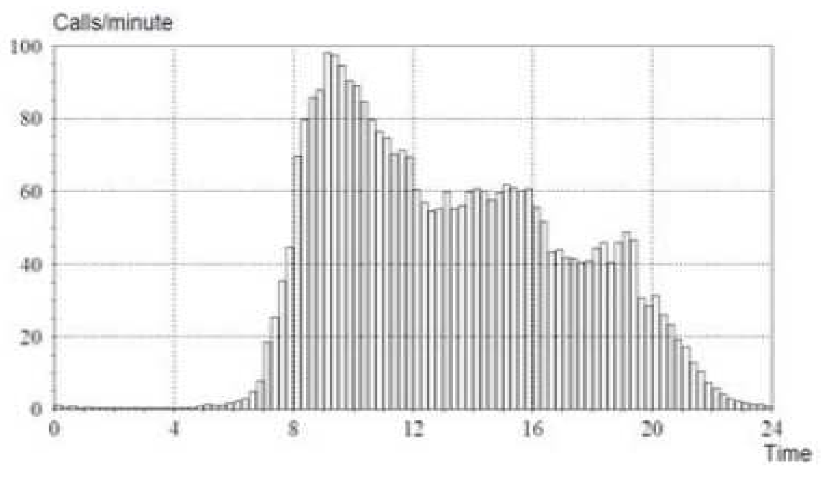
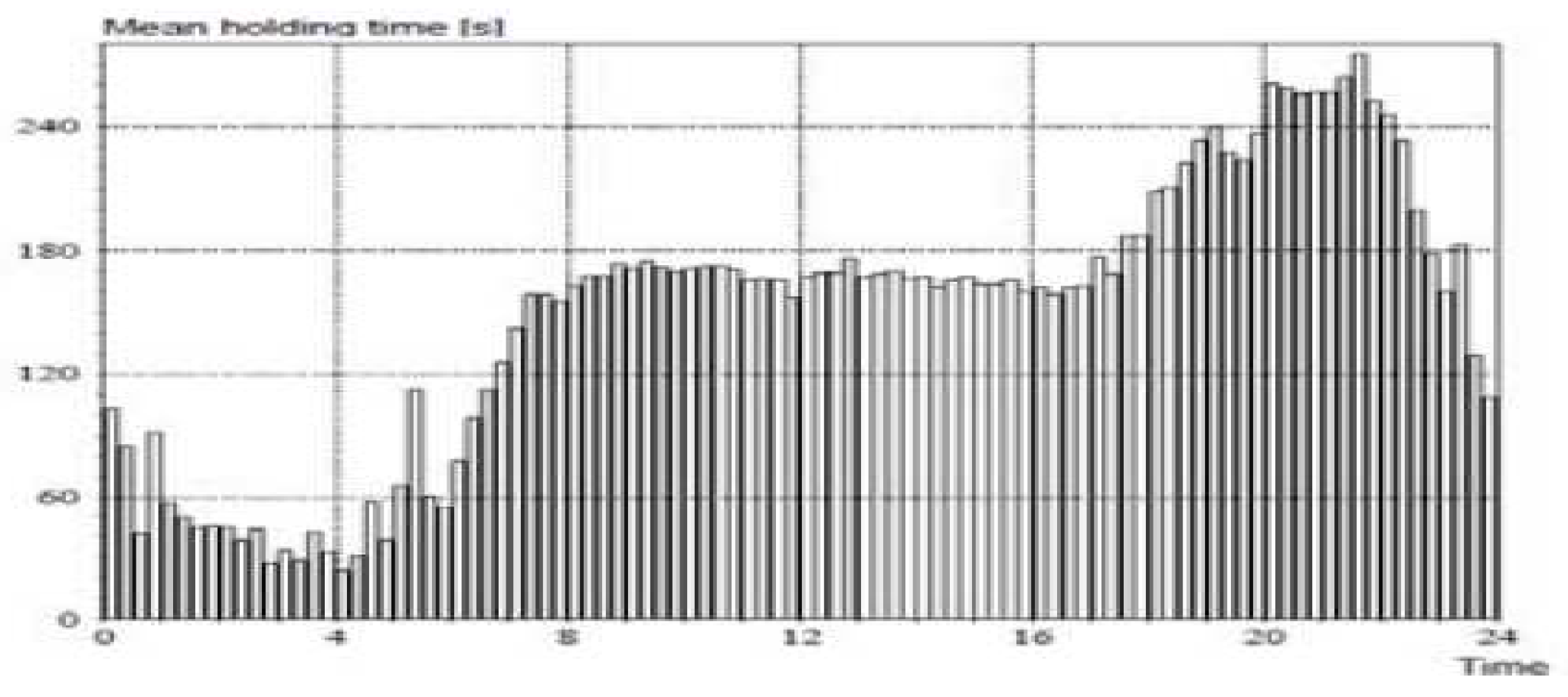
Both Figure 1 and Figure 2(c.f., [2]) provide two real life applictions of Time Varying queueing systems. In Figure 1, the Mean number of calls per minute at a central office switch – measured in 15 minutes intervals averaged over 10 work days are observed . Furthermore, Figure 2 describes the associated Mean call holding times.

3. The $G I / M / 1$

Queueing Model

This section discusses the

G I / M / 1

queueing model, in which the service time has an exponential distribution, and the inter-arrival process has an identical distribution with successive inter-arrival periods. Let

A (t)

stand for the distribution of inter-arrival times. The

G I / M / 1

queue's steady state probability for the number of customers a new arrival finds in the system is a geometric distribution:

π_{n} = (1 - σ) σ^{n}

(10)

σ

(

1 > σ > 0)

uniquely solves:

σ = f_{a}^{*} (s) |_{s = μ (1 - σ)}

(11)

where

f_{a}^{*} (s)

is the Laplace-Stieltjes transform of the inter-arrival time distribution

A (t)

, that is:

f_{a}^{*} (s) = L^{*} (A (t)) = \int_{0}^{\infty} e^{- s t} d A (t)

(12)

Notably,

σ = 1

solves (11),

a n d t h e s t a t e v a r i a b l e

x

reads as:

x = \frac{λ}{μ (1 - σ)} = \frac{ρ}{(1 - σ)}

(13)

In determining the PSFFA model, equation (13) re-writes to

ρ (t) = x (t) μ (1 - σ (t))

(14)

We believe that the non-stationary load will exhibit sinusoidal mean behaviour, which will describe the cyclic load pattern over a specified time period (for example, day) in accordance with the prior research on non-stationary analysis of communication networks[4,5,6]], namely

λ (t) = A + B s i n (w t + D),

for more details see[7,8].

Thus, the required model reads as:

x^{.} (t) = μ x (t) (1 - σ (t)) + λ (t)

(15)

We can numerically solve (15) to visualize the queue’s time varying behaviour.

Depending on the inter-arrival distribution

A (t),

the precise process for figuring out will vary, although it usually involves a root-finding approach like Laguerre's method. The time varying

D / M / 1

queue’s

G I / M / 1

PSFFA model reads:

x^{.} (t) = - μ x (t) (1 - σ (t)) + λ (t), σ (t) = e^{\frac{μ}{λ (t)} (σ (t) - 1)}

(16)

The

D / M / 1

case in equation (16) corresponds to a deterministic arrival process where the inter-arrival distribution

A (t)

is a delta function (i.e.,

d A (t) = f_{a} (t) d t a n d f_{a} (t) = δ (t - \frac{1}{λ})

)

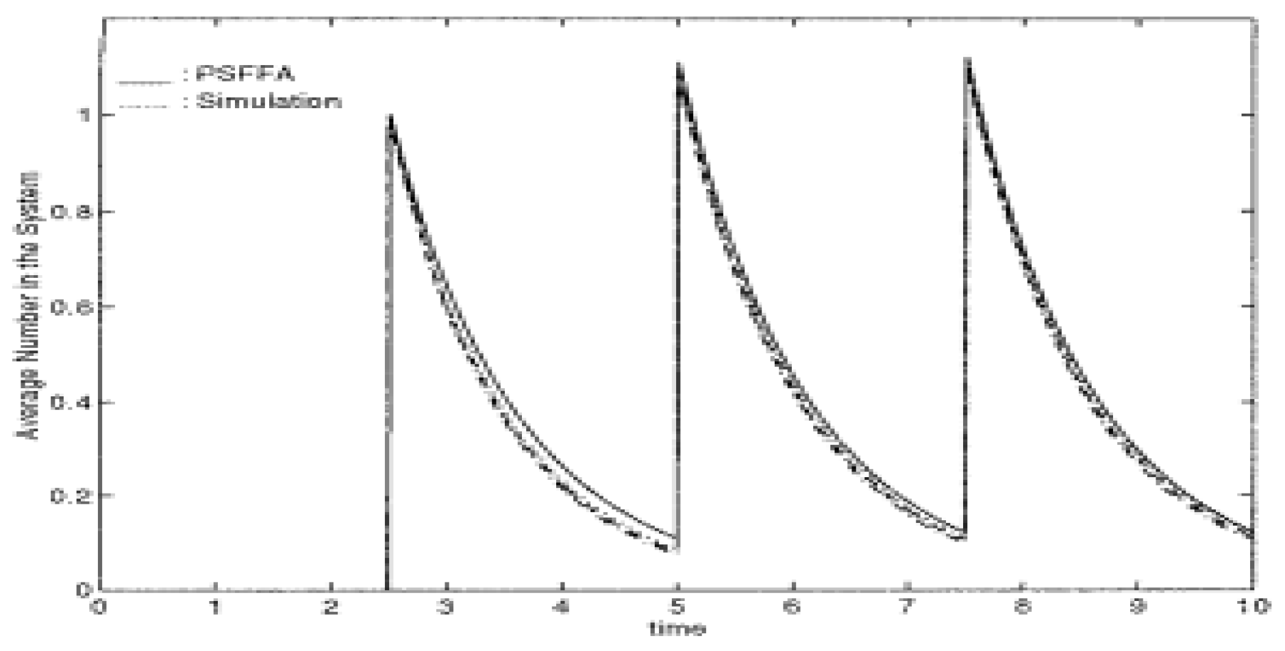
Figure 3. c.f.,[1]): Comparing

D / M / 1

model with low load simulation.

Figure 3. c.f.,[1]): Comparing

D / M / 1

model with low load simulation.

4. Impact of the time-dependent root parameter (c.f., (16)) on the stability of $t h e n o n - s t a t i o n a r y t h e D / M / 1 q u e u e G I / M / 1$ PSFFA model

Theorem 1 The time-dependent root parameter (c.f., (16)), $σ (t), 1 > σ (t) > 0$ if and only if the underlying queue’s $G I / M / 1$ PSFFA model is stable.
Proof
Sufficiency: Let the time-dependent root parameter, $σ (t) b e s u c h t h a t 1 > σ (t) > 0$ . By (3.7), it follows that:

$ρ (t) = \frac{λ (t)}{μ} = \frac{(σ (t) - 1)}{l n (σ (t))}$

(17)

It is well known that (c.f., [9])

1 - \frac{1}{x} \leq \ln (x) \leq x - 1 f o r x \geq - 1

(18)

Engaging (17) and (18), it follows that:

ρ (t) = \frac{λ (t)}{μ} \leq 1

(19)

It is noted that:

{l i m}_{σ (t) \to 1} \frac{(σ (t) - 1)}{l n (σ (t))} = {l i m}_{σ (t) \to 1} \frac{1}{\frac{1}{(σ (t))}} = 1 (L ’ Hopital ’ L rule)

(20)

This implies

ρ (t) = 1

. This completely proves sufficiency.

This implies stability of the underlying queue.

Necessity: Let

ρ (t) > 1 . A s s u m e t h a t 1 > σ (t) > 0 .

By (17) and (18), we have

1 - \frac{1}{σ (t)} < l n (σ (t)) < (σ (t) - 1)

(21)

Hence, it follows that:

0 < {(σ (t) - 1)}^{2}

(22)

Therefore,

σ (t) > 1

(23)

This proves necessity.

5. Numerical portraits

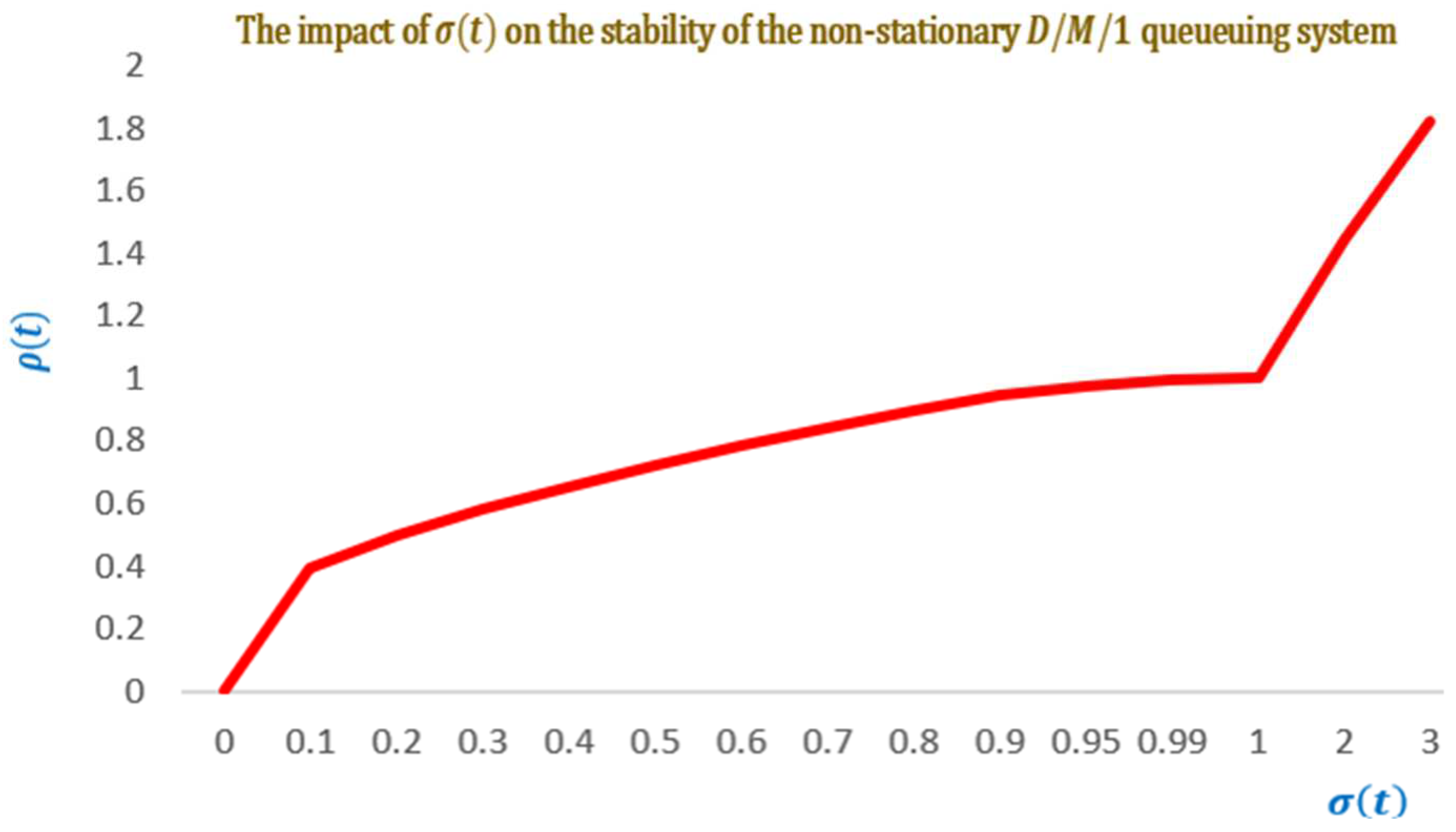
It is observed from Figure 4, that the time-dependent root parameter has a significant impact on the underlying queue’s stability. Moreover, the progressive increase of the time dependent server utilization,

ρ (t)

implies the increase of the time dependent root parameter. We can see that:

{l i m}_{σ (t) \to 0} \frac{(σ (t) - 1)}{l n (σ (t))} = {l i m}_{σ (t) \to 0} \frac{- 1}{\frac{1}{(σ (t))}} = 0 (L ’ Hopital ’ L rule)

(24)

and

{l i m}_{σ (t) \to \infty} \frac{(σ (t) - 1)}{l n (σ (t))} = {l i m}_{σ (t) \to \infty} \frac{1}{\frac{1}{(σ (t))}} = \infty (L ’ Hopital ’ L rule)

(25)

Figure 4. The impact of time-dependent root parameter on the stability for the underlying queue.

6. Some PSFFA applications to IoT

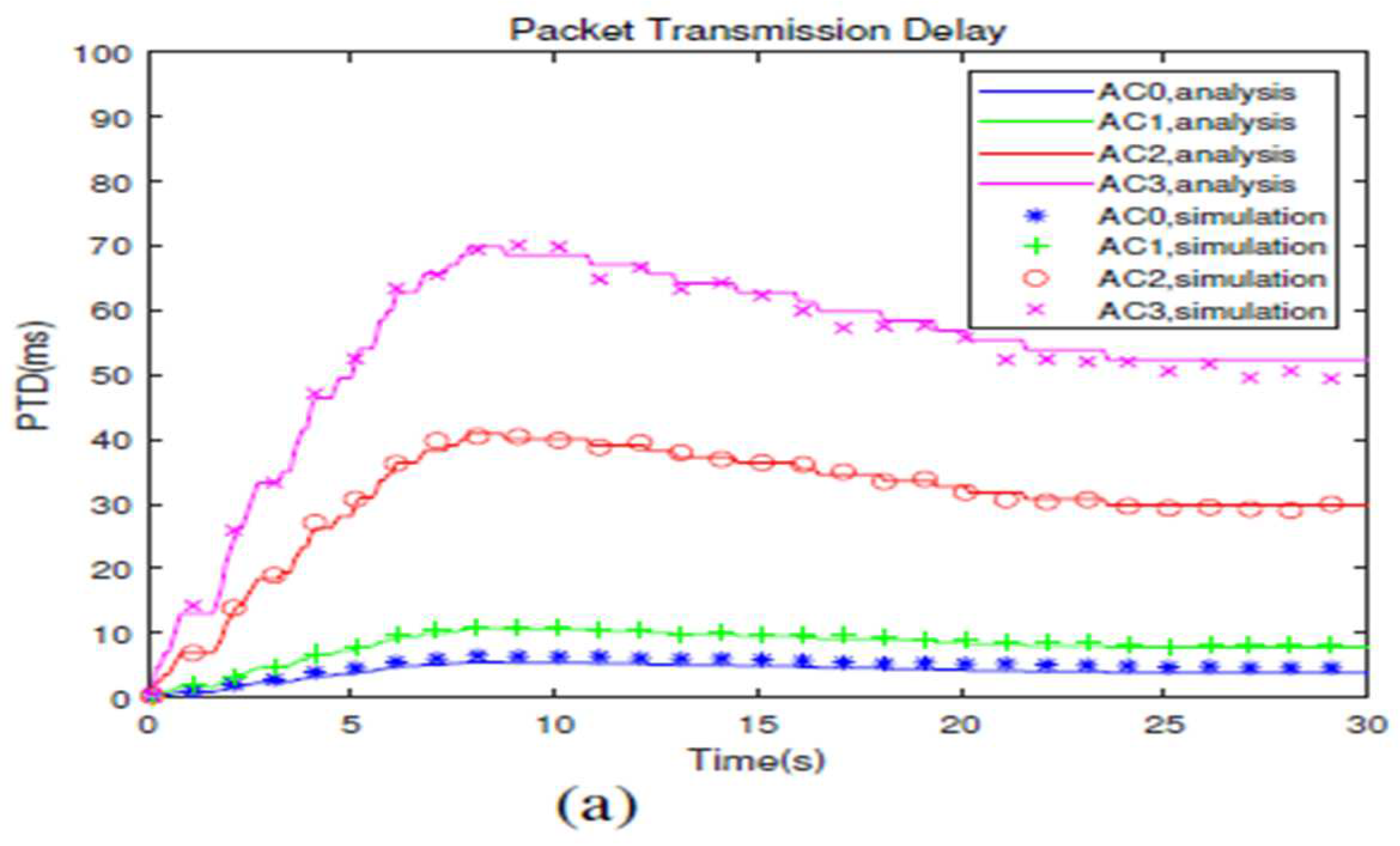
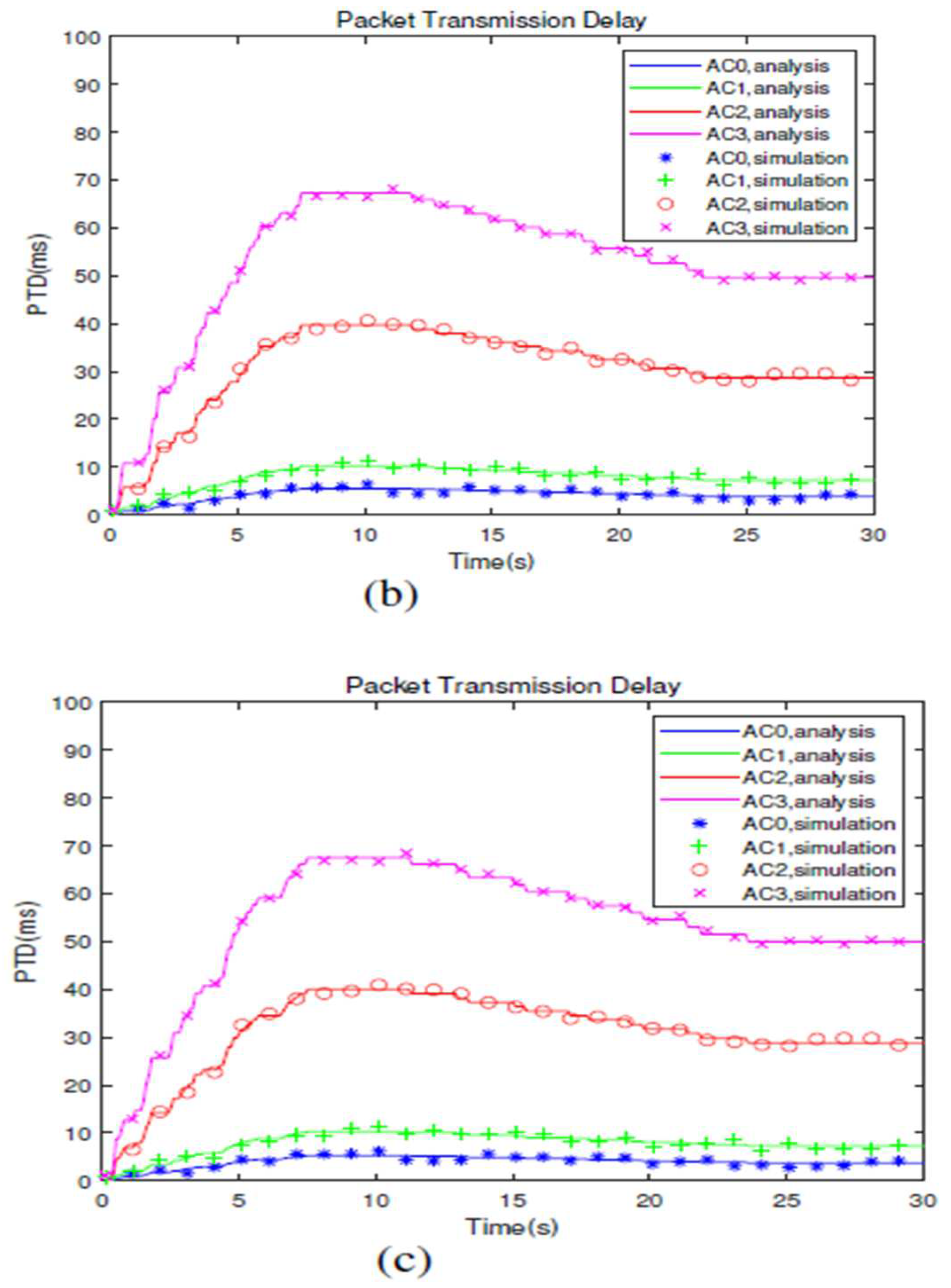
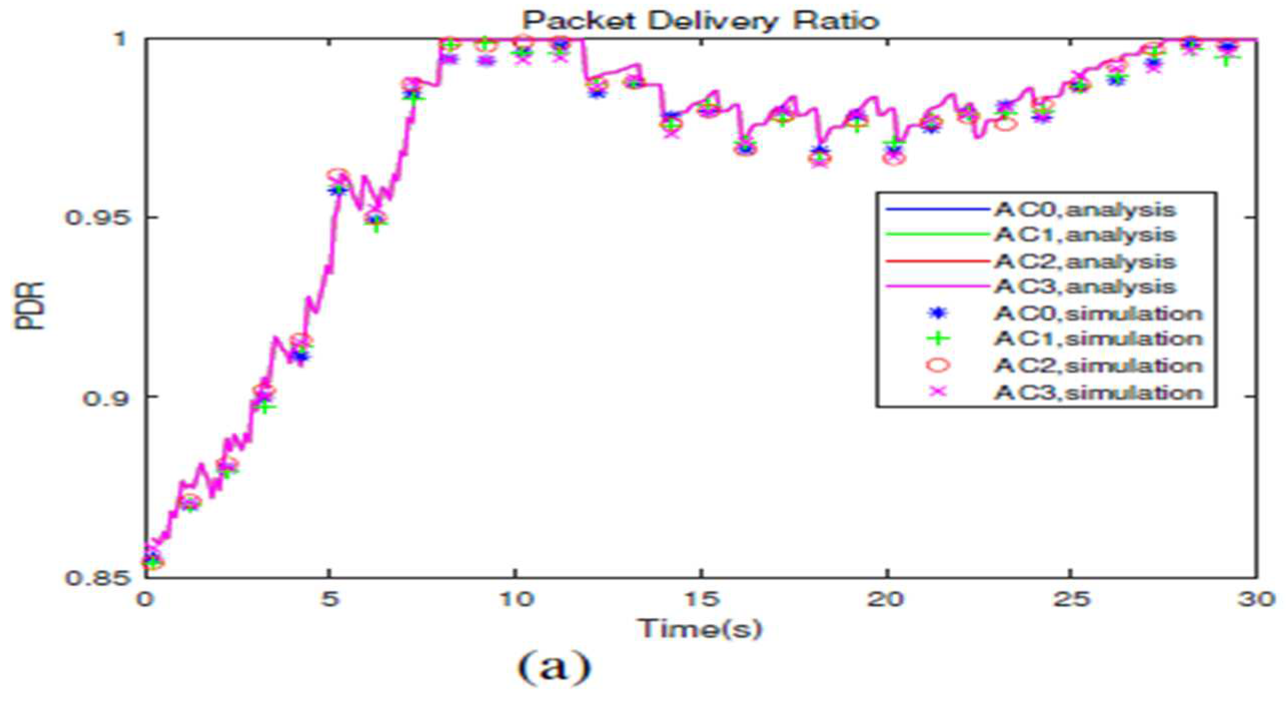
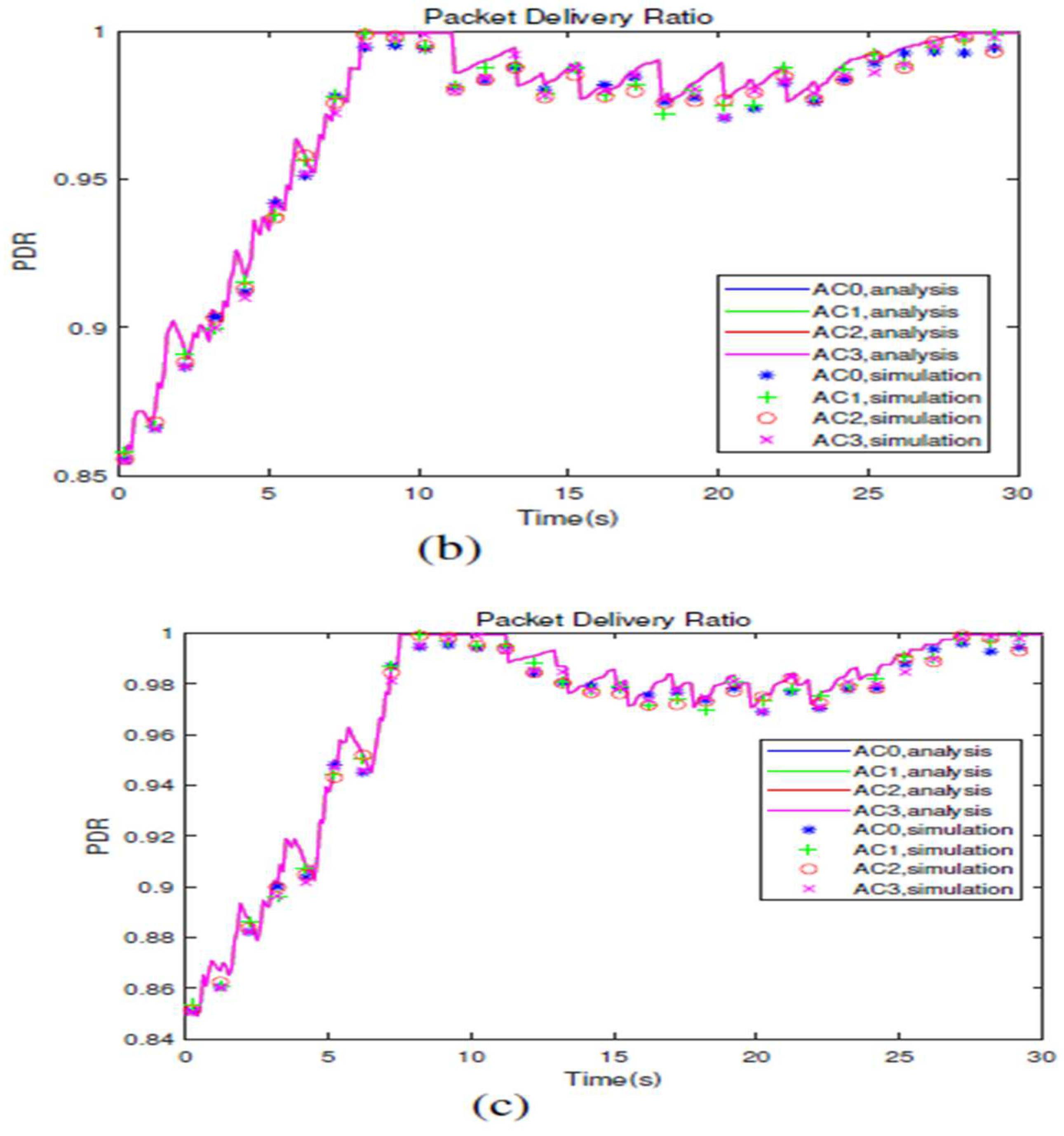
By describing how vehicles in a platoon use 802.11p communication to exchange messages and change their movement characteristics at intersections, a time-dependent model for assessing the platooning communications’ effectiveness at intersections phase was thoroughly investigated[10]. The model evaluates the effectiveness of platooning communications and addresses potential safety concerns by considering variables including vehicle behaviours, traffic signals, and the changing connectivity among vehicles.

The authors [10] used PSFFA to describe the transmission queue’s dynamic behaviour in platooning communications. They also create models that characterise the continuous backoff freeze and four access categories (ACs) of 802.11p as they relate to the time-dependent access procedure.

For 802.11p communication in platooning situations at junctions, the authors created models. [10] consider continual backoff freezing and use the PSFFA to describe the gearbox queue’s dynamic behaviour. The access process with its four Access Categories (ACs), they also use a z-domain linear model was demonstrated by [10].

The display of time-dependent packet transmission delay and packet delivery ratio of four Acs can be visualized by Figures 5a, 5b, 5c, 6a,6b and 6c, respectively.

The findings of a study[11] into the variables influencing queue utilisation dynamics on routers in telecommunication networks. The investigation shows that the average queue length reaches a steady state value following a transient process lasting from a few to tens of seconds when utilising a dynamic model, specifically PSFFA. It is advised to calculate the average queue length using steady state estimations only after the transient process has finished and a more precise differential model may be used.

To accurately predict the average queue length while analysing the average queue length and Quality of Service[11] in a network, a dynamic model with a nonlinear differential equation must be used. Only when the transient process has ended, and the length of the transient process is controlled by variables like flow rate, router interface capacity, and service discipline, are steady-state estimations useful for determining the average queue length. A better choice of queuing models and smaller packet sizes can further hasten the average queue length's convergence.

7. Conclusion and future work

An exposition is undertaken to reveal the significant impact of

σ (t), 1 > σ (t) > 0

on the stability of

D / M / 1

queueing system’s

G I / M / 1

PSFFA stability. It has been shown that the time-dependent root parameter has a significant impact on the stability of the underlying non-stationary

D / M / 1

queueing system. Moreover, the progressive increase of the time dependent server utilization,

ρ (t)

implies the increase of the time dependent root parameter. More fundamentally, some interesting PSFFA applications to IoT are provided. Future work involves further investigation of the impact of

σ (t), 1 > σ (t) > 0

on the stability of

G / M / 1

PSFFA model of the

n o n - s t a t i o n a r y E_{k} / M / 1 a n d I P P / M / 1

queueing systems.

References

Wang, W-P., Tipper, D., and Banerjee, S. 1996: A simple Approximation for Modelling Non-Stationary Queues, IEEE.
Poryazov S, Andonov V, Saranova E. Methods for Modelling of Overall Telecommunication Systems. Research in Computer Science in the Bulgarian Academy of Sciences. 2021:325-61.
Zhu M, Gao S, Tu G, Chen D. Multi-Access Edge Computing (MEC) Based on MIMO: A Survey. Sensors. 2023 Apr 11;23(8):3883. [CrossRef]
Mageed IA, Zhang Q, Modu B. The Linearity Theorem of Rényian and Tsallisian Maximum Entropy Solutions of The Heavy-Tailed Stable M/G/1 Queueing System entailed with Potential Queueing-Theoretic Applications to Cloud Computing and IoT. electronic Journal of Computer Science and Information Technology. 2023 Apr 23;9(1):15-23.
Grassmann, W.K. 1990: Computational Methods in Probability Theory, Handbook in Operations Research and Management Science, Vol.2, North Holland.
Mageed IA, Zhang KQ. Solving the open problem for GI/M/1 pointwise stationary fluid flow approximation model (PSFFA) of the non-stationary D/M/1 queueing system. electronic Journal of Computer Science and Information Technology. 2023 Apr 23;9(1):1-6.
Chang J, Chan HK, Lin J, Chan W. Non-homogeneous continuous-time Markov chain with covariates: Applications to ambulatory hypertension monitoring. Statistics in Medicine. 2023 May 30;42(12):1965-80. [CrossRef]
GRASSMANN, WK. Finding Transient Solutions in Markovian Event Systems Through Numerical Solution of Markov Chains. 2021 Jun 30:357.
Kozma, L. 2020: Useful inequalities, online source, available at http://www.Lkozma.
Wu Q, Zhao Y, Fan Q. Time-dependent performance modeling for platooning communications at intersection. IEEE Internet of Things Journal. 2022 Mar 22;9(19):18500-13. [CrossRef]
Yeremenko O, Lebedenko T, Vavenko T, Semenyaka M. Investigation of queue utilization on network routers by the use of dynamic models. In2015 Second International Scientific-Practical Conference Problems of Info communications Science and Technology (PIC S&T) 2015 Oct 13 (pp. 46-49). IEEE.

Figure 1.

Figure 2.

Figure 5. The packet transmission delay that is time dependent. A left turn, a straight shot, or a right turn, respectively[10].

Figure 6. The proportion of time-dependent packet deliveries. A left turn, a straight shot, or a right turn, respectively[10].

Disclaimer/Publisher’s Note: The statements, opinions and data contained in all publications are solely those of the individual author(s) and contributor(s) and not of MDPI and/or the editor(s). MDPI and/or the editor(s) disclaim responsibility for any injury to people or property resulting from any ideas, methods, instructions or products referred to in the content.

© 2024 by the authors. Licensee MDPI, Basel, Switzerland. This article is an open access article distributed under the terms and conditions of the Creative Commons Attribution (CC BY) license (http://creativecommons.org/licenses/by/4.0/).

Copyright: This open access article is published under a Creative Commons CC BY 4.0 license, which permit the free download, distribution, and reuse, provided that the author and preprint are cited in any reuse.

MDPI Initiatives

Important Links

Choose an area of interest and we will send you notifications of new preprints at your preferred frequency.

Disclaimer

Effect of the root parameter on the stability of the Non-stationary D/M/1 queue’s GI/M/1 model with PSFFA applications to the Internet of Things (IoT)

Abstract

1. Introduction

2. PSFFA

3. The G I / M / 1

4. Impact of the time-dependent root parameter (c.f., (16)) on the stability of t h e n o n − s t a t i o n a r y t h e D / M / 1 q u e u e G I / M / 1 PSFFA model

5. Numerical portraits

6. Some PSFFA applications to IoT

7. Conclusion and future work

References

MDPI Initiatives

Important Links

Subscribe

3. The $G I / M / 1$

4. Impact of the time-dependent root parameter (c.f., (16)) on the stability of $t h e n o n - s t a t i o n a r y t h e D / M / 1 q u e u e G I / M / 1$ PSFFA model