Preprint
Article

Machine Learning Predictive Analysis of Liquefaction Resistance for Sandy Soils Enhanced by Chemical Injection

Altmetrics

Downloads

69

Views

25

Comments

0

A peer-reviewed article of this preprint also exists.

Submitted:

26 January 2024

Posted:

26 January 2024

You are already at the latest version

Alerts
Abstract
The objective of this study was to investigate the liquefaction resistance of chemically improved sandy soils in a straightforward and accurate manner. Using only the existing experimental databases and artificial intelligence, the goal was to make predictions without conducting physical experiments. Emphasis was placed on the significance of data from 20 loading cycles of cyclic undrained triaxial tests to determine the liquefaction resistance and the contribution of each explanatory variable. Different combinations of explanatory variables were considered. Regarding the predictive model, it was observed that a case with the liquefaction resistance ratio as the dependent variable and other parameters as explanatory variables yielded favorable results. In terms of exploring combinations of explanatory variables, it was found advantageous to include all variables as doing so consistently resulted in a high coefficient of determination. The inclusion of the liquefaction resistance ratio in the training data was found to improve the predictive accuracy. In addition, the results obtained when using a linear model for the prediction suggested the potential to accurately predict the liquefaction resistance using historical data.
Keywords: 
Subject: Engineering  -   Civil Engineering

1. Introduction

The significant structural damage often caused by the settlement or tilting of structures, due to the liquefaction of saturated sandy soils during large earthquakes, has long been a major concern in the field of geotechnical engineering, as shown in Figure 1. This phenomenon, which can have serious consequences, was particularly documented in a seminal studies [1,2,3,4]. The sudden instability of the ground during such events can lead to the catastrophic destruction of buildings and infrastructures, resulting in significant economic losses as well as the tragic loss of human life. This critical issue was further highlighted [5,6]. These concerns have led to a significant increase in the study and development of activities aimed at improving liquefaction resistance and developing other mitigation methods. This focus was particularly highlighted by the groundbreaking work [7,8], which contributed to a better understanding of these challenges.
In response to these critical challenges, the chemical injection method has emerged as a prominent and innovative solution for mitigating subsurface liquefaction risks [9,10,11,12,13]. This technique involves injecting chemical agents into sandy soils to increase their stability and cohesion. However, the effective implementation of this method and the accurate execution of designs depend heavily on the availability of precise and reliable data on the liquefaction resistance of the targeted chemically treated sandy soils [14,15,16,17,18]. Traditionally, liquefaction resistance has been assessed using cyclic undrained triaxial tests, which are fundamental to building comprehensive databases reflecting a variety of test conditions and results [19,20,21,22,23,24]. Despite their critical importance in understanding soil behavior, these tests are often time-consuming, expensive, and labor-intensive. In addition, they are limited by the diverse nature of the properties of sandy soils found in different geographic regions, requiring a large number of experiments for a thorough and comprehensive data collection [25,26,27].
To address these challenges and limitations, the present study introduces a novel and state-of-the-art approach that employs machine learning and ensemble learning techniques [28,29,30]. The authors of this study propose a predictive model for evaluating the liquefaction resistance of sandy soils treated with solution-type chemical agents. This model is a synergistic combination of existing experimental data and advanced algorithms with artificial intelligence (AI) [31,32,33,34]. This innovative approach makes it possible to predict the liquefaction resistance of sandy soils without the need to conduct additional laborious and costly experiments. The method is not only efficient, but also cost-effective, providing significant advances in the formulation of liquefaction mitigation strategies and enhancing risk assessment capabilities in geotechnical engineering [35]. The methodology of this study begins with the meticulous collection and analysis of data from cyclic undrained triaxial tests. The data form the basis of the machine-learning database used in the study. Employing ensemble learning techniques, the authors successfully integrate the results of different prediction models to produce more accurate and reliable predictions. The primary goal of this study is to comprehensively assess the risk of sandy soil liquefaction and to provide reliable guidance for the design and implementation of chemical injection methods. It is expected that the development of this innovative non-experimental prediction method will contribute significantly to the sustainable development and advancement of geotechnical engineering practices. This approach not only minimizes the environmental impact, but also significantly reduces the time and costs associated with traditional soil testing methods. By introducing AI as a transformative tool in geotechnical engineering for predicting liquefaction resistance [36,37], this study aims to revolutionize the field and to improve the safety and stability of sandy soils in earthquake-prone areas.
The application of AI in this context is particularly noteworthy, as it represents a paradigm shift in how geotechnical engineering challenges are addressed. By harnessing the power of machine learning, the study bypasses the limitations of traditional experimental methods. The AI-driven model is able to synthesize large amounts of experimental data, learn from different soil conditions, and adapt to different chemical treatments. This leads to a more holistic understanding of soil behavior under seismic activity, providing engineers with a powerful tool for predicting the soil response in real-world scenarios. Of particular importance in this study is the use of ensemble learning techniques. Ensemble learning involves combining multiple machine learning models to improve prediction accuracy [38], thereby reducing the likelihood of erroneous predictions that could lead to unsafe engineering practices. This approach ensures that the predictive model is not based on a single data set or algorithm, but is a robust composite of multiple predictive insights, resulting in a more reliable and trustworthy predictive model. In addition, the study′s approach to integrating AI with traditional geotechnical engineering practices is an exemplary model of interdisciplinary innovation. By bridging the gap between advanced computational techniques and practical engineering applications, the study sets a precedent for future studies in the field. It demonstrates the potential of AI to improve the accuracy and efficiency of engineering solutions, thereby contributing to the development of safer and more resilient infrastructures. The study not only addresses the immediate challenge of predicting and mitigating the liquefaction of sandy soils, but also opens new avenues for study and innovation in geotechnical engineering. By harnessing the power of AI and machine learning, it presents a forward-looking approach that could revolutionize the field, leading to more sustainable, efficient, and safer engineering practices [39]. This study not only contributes to the academic body of knowledge, but also has practical implications for the construction industry, urban planning, and disaster risk management, especially in earthquake-prone regions.

2. General Evaluation and Countermeasures to Liquefaction of Sandy Soils

2.1. Chemical Injection Method

The liquefaction of sandy soils during seismic events is a significant challenge in geotechnical engineering [40,41]. It poses a risk to the stability and integrity of structures built on such soils. In response, chemical injection has emerged as a promising technique for mitigating liquefaction in sandy soils [9,10,11,12,13].
Liquefaction occurs when saturated sandy soils lose their strength and stiffness in response to an applied stress, such as an earthquake, resulting in fluid-like behavior [42]. The chemical injection method, also known as soil grouting, involves injecting chemical solutions into soils to improve their physical and mechanical properties, thereby increasing their resistance to liquefaction.
The chemical injection process typically involves the use of materials such as silicates, polyurethanes, or acrylamides. When injected into a soil, these chemicals react with the soil particles or with each other to form a solidified matrix that binds the soil particles together, increasing their density and shear strength. One common approach is to use sodium silicate, a water-soluble silicate that reacts with calcium chloride to form a gel-like substance. This substance fills the voids between the soil grains, reducing porosity and increasing soil cohesion. Another approach is to use organic polymers that solidify when injected, creating a network of polymer chains that bind the soil particles together.
Chemical injection has several advantages. It is a relatively quick process compared to other soil stabilization methods and can be applied to specific areas without the need for an extensive excavation or the disruption of existing structures. In addition, the method can be tailored to different soil types and conditions [13].
Despite its advantages, the chemical injection method also faces several challenges and limitations. The use of chemicals raises environmental concerns. Some chemicals used in the process can be harmful to the environment, especially if they leach into the groundwater. Selecting environmentally friendly chemicals that do not compromise soil stability is critical. In addition, the long-term effectiveness of the treatment is uncertain. Over time, the injected chemicals may degrade or the bond between soil particles may weaken, reducing the effectiveness of the treatment. Achieving the uniform distribution of the chemical solution throughout the soil is challenging. Inhomogeneous treatment can result in uneven soil properties that may not effectively mitigate liquefaction hazards. Moreover, the process can be costly, especially for large-scale applications. The cost of the chemicals and the need for specialized equipment and personnel can be significant. Finally, it is also noted that not all sandy soils are suitable for chemical injection. The method is less effective in soils with high organic content or those that are too coarse or too fine. Effective monitoring and quality control are essential to ensuring successful treatment. This includes monitoring the distribution of chemicals, the reaction process, and the final soil properties.
The chemical injection method for liquefaction mitigation in sandy soils offers a viable solution for improving soil stability in seismic areas [43]. However, it is imperative to address the environmental, technical, and economic challenges associated with this method. Future studies should focus on developing environmentally friendly chemicals, improving application techniques for uniform soil treatment, and evaluating the long-term performance of treated soils. With advances in technology and a better understanding of soil behavior, chemical injection has the potential to become a more effective and sustainable option for liquefaction mitigation in sandy soils.

2.2. Cyclic Undrained Triaxial Test

In geotechnical engineering, the cyclic undrained triaxial test is a critical method for evaluating the liquefaction resistance of chemically treated sandy soils. This test simulates the stress conditions experienced by soils during seismic events and provides important information on the behavior of the soils under such conditions [19,20,21,22,23,24].
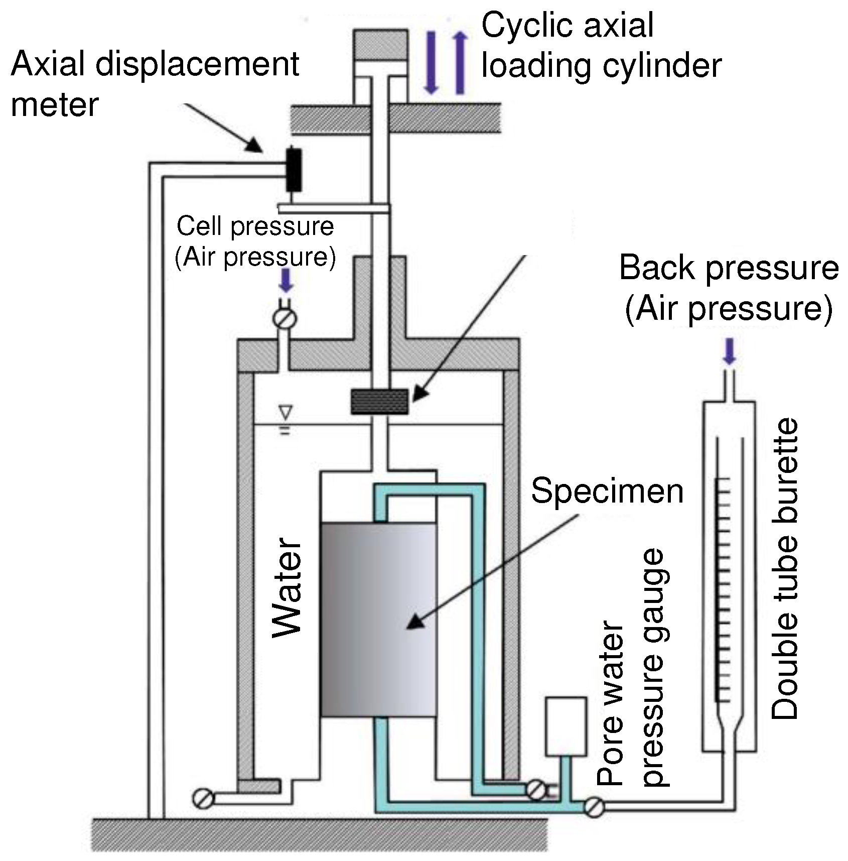
Liquefaction is the phenomenon in which saturated sandy soils significantly lose their strength and stiffness in response to an applied load, such as seismic shaking, causing them to behave like a liquid. The cyclic undrained triaxial test is a laboratory test designed to evaluate the resistance of soils to liquefaction, which is particularly important for soils that have been treated with chemical agents for stabilization. Figure 2 shows the typical appearance of the cyclic undrained triaxial test.
The test involves the cyclic loading of a cylindrical soil sample in a triaxial chamber. The soil sample is first saturated and then subjected to axial cyclic loading at a controlled frequency and amplitude. The test is undrained, meaning that no water can enter or leave the soil sample during the test. This condition simulates the rapid loading that occurs during earthquakes. Parameters, such as axial stress, axial strain, pore water pressure, and volume change, are recorded. The number of cycles the soil can withstand before failure (defined by a certain level of strain or pore pressure) is used to evaluate its resistance to liquefaction.
The cyclic undrained triaxial test is widely recognized for its ability to replicate the stress conditions experienced by soils during earthquakes. It provides valuable data on the behavior of chemically treated soils, including the stiffness, strength, and pore pressure response, which are critical for evaluating the liquefaction potential [19,20,21,22,23,24].
Despite its advantages, the cyclic undrained triaxial test faces several challenges. Obtaining and preparing undisturbed soil samples for testing is challenging. Sample disturbance can significantly affect the test results, making it difficult to accurately represent the in-situ soil conditions. Each test is conducted on a small-scale soil sample, which may not accurately represent the behavior of the soil mass in the field due to scale effects. For chemically treated soils, it is difficult to ensure the uniform distribution of the chemical agent throughout the sample. Inconsistent treatment can lead to variable results that do not accurately reflect the true behavior of the treated soil. The test is complex and requires sophisticated equipment and skilled personnel, making it expensive and time-consuming. Accurate measurement of the pore water pressure during the test is critical, but can be challenging, especially in sands with low permeability. It is difficult to ensure the repeatability and reliability of the test results due to the inherent variability of the soil properties and the sensitivity of the test to experimental conditions.
The cyclic undrained triaxial test is an essential tool for evaluating the liquefaction resistance of chemically treated sandy soils. However, overcoming the challenges associated with sample preparation, scale effects, chemical interactions, test complexity, and measurement accuracy is critical to obtaining reliable results. Future advances in test procedures, equipment, and analytical methods are needed to overcome these challenges. By improving the cyclic undrained triaxial test, it can continue to be a valuable method for evaluating the effectiveness of chemical treatments for mitigating the liquefaction hazards of sandy soils.

2.3. Liquefaction Resistance Ratio

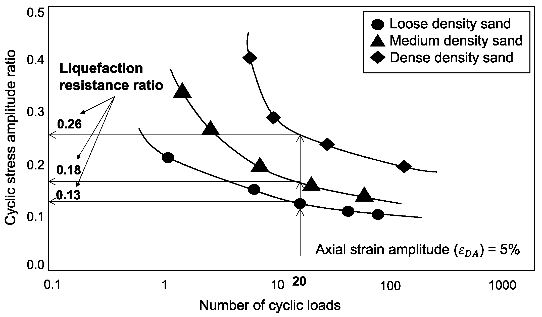
The concept of the liquefaction resistance ratio, often derived from the cyclic undrained triaxial test, is a critical parameter in geotechnical engineering, particularly in assessing the stability of soils under seismic conditions. This ratio is a measure of a soil′s ability to resist liquefaction, a phenomenon in which saturated soil loses much of its strength and stiffness in response to an applied stress, such as an earthquake, causing it to behave like a fluid. In the context of the cyclic undrained triaxial test, the liquefaction resistance ratio is defined as the ratio of the cyclic stress required to cause liquefaction in a soil sample to the maximum cyclic stress experienced by the soil during an earthquake [14,15,16,17,18]. Liquefaction in this test is typically identified by a specific criterion, such as reaching a predetermined level of axial strain or a significant increase in pore water pressure, indicating a loss of soil strength. The cyclic undrained triaxial test involves subjecting a cylindrical soil sample, saturated and confined in a triaxial chamber, to controlled cyclic axial loading. The loading simulates the stress conditions that the soil would experience during seismic events. The cyclic stress required to induce liquefaction is determined by gradually increasing the stress amplitude of the loading cycles until the soil sample reaches the failure criterion. The liquefaction resistance ratio is an index that indicates the resistance of the sandy soil to liquefaction. Specifically, it refers to the cyclic stress amplitude ratio when the axial strain amplitude reaches 5% or the excess pore water pressure ratio reaches 95% and the number of cyclic loads is 20 [13]. This index is calculated from the liquefaction intensity curve [13,44] obtained as a result of the cyclic undrained triaxial test, as shown in Figure 3. The cyclic undrained triaxial test simulates liquefaction phenomena under compacted and undrained conditions in a testing machine. The collected undisturbed specimen is compacted under the original effective confining pressure, subjected to cyclic shear stress equivalent to the stress during an earthquake, and tested. During the test, experiments are performed at multiple cyclic stress levels and the number of cyclic loads at which both axial strain amplitudes reach 5% is determined. A liquefaction intensity curve is constructed from this data.

3. Machine Learning Predictive Analysis

3.1. Ensemble Learning

Ensemble learning methods use multiple machine learning algorithms to produce weakly predictive results based on features extracted through a variety of projections on the data and fuse the results with various voting mechanisms to achieve a better performance than that obtained by any constituent algorithm alone [45]. Neural networks have attracted attention in the field of machine learning due to their high expressiveness in modeling nonlinear data. On the other hand, gradient boosting decision trees excel in terms of interpretability and accuracy. It is expected that the combination of these two methods will improve the predictive accuracy of the model.
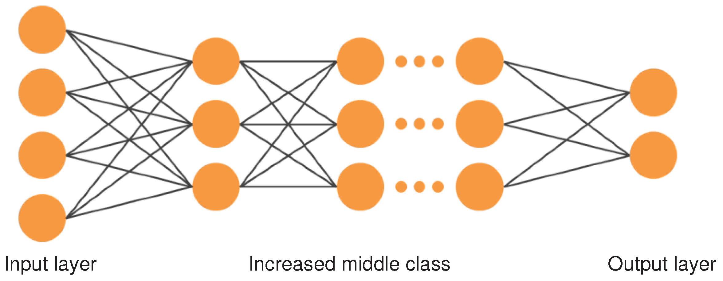
A neural network is an interconnected collection of simple processing elements, units or nodes, whose functionality is loosely based on the animal neuron. The processing capability of the network is stored in the inter-unit connection strengths or weights, which are obtained through a process of adaptation to, or learning from, a set of training patterns [46,47,48,49]. A model with many hidden layers is called deep learning. Multiple inputs and outputs are possible, and neural networks enable prediction, judgment, and classification. As shown in Figure 4, data are input into the input layer, the features are input with indicators of the data, and the final results are calculated by inputting neurons into the output layer.
The gradient boosting decision tree is an algorithm that learns multiple decision trees sequentially, using the residuals from the previous decision tree in the learning process of the next decision tree. This method also uses a gradient descent to minimize the errors in the predicted values [50,51,52].
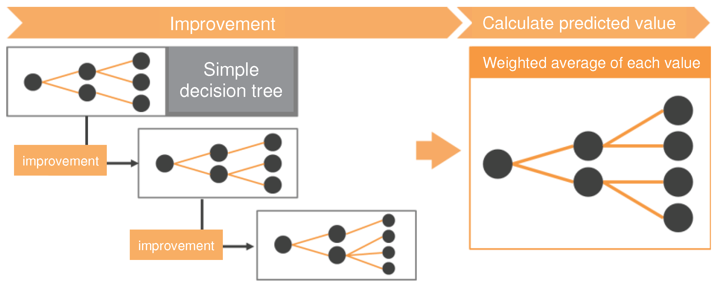
The ensemble model proposed in this study combines two models: a neural network and a gradient boosting decision tree. As shown in Figure 5, it determines the weighted average of the predictions from these models to generate the final prediction. Both models are known for their high predictive performance in terms of tabular training data, and it is expected that the combination of these models, through ensemble modeling, will further improve the accuracy.
Before constructing the ensemble model, a method is used to optimize the generalization ability of each model. Specifically, the training data are divided into several subsets, and a technique called random search is used for cross-validation to optimize the hyperparameters.

3.2. Preparation of Dataset

Data sets play a crucial role in the implementation of machine learning. They are divided into two main categories: training data and test data. Training data are used for model training, which is the necessary basis for acquiring the generalization ability.

3.2.1. Details of training data

In this study, data from cyclic undrained triaxial tests on chemically improved sandy soils, conducted to determine the liquefaction resistance, were used. These data include specimen conditions, test conditions, and test results. Specifically, the variable elements shown in Table 1 were extracted from previous test records to form the training data. A total of 272 specimens from 68 cases of cyclic undrained triaxial tests were used. One case corresponds to one site. In order to obtain the liquefaction resistance as shown in Figure 3, at least four specimens must be used for the cyclic undrained trial tests conducted for each case (each site). All 272 specimens were chemically improved sandy soils with 6%, 9%, and 12% silica concentrations, with four specimens being collected from each of the 68 sites.

3.2.2. Details of test data

The test data in this study are based on the above training data. However, the test data exclude the target variables of the training data and mainly consist of explanatory variables from the training data.

3.3. Distinguishing Explanatory and Target Variables

In this study, the training data are used to train an ensemble model and, after the learning process, predictions are made by inputting test data. During this process, the predicted values are compared with the target variables of the training data to validate the predictive performance of the machine learning model. In this study, the distinction between the explanatory variables and the target variables is made for four cases, namely, Case-1, Case-2, Case-3, and Case-4, as shown in Table 2. An example of the training data used in this study, i.e., data for 2 of the 272 specimens, are presented in Table 3. The target variable for Case-3 and Case-4 is the same. The difference is that Case-3 makes predictions without liquefaction resistance, while Case-4 makes them with liquefaction resistance.

3.4. Evaluation of Prediction Accuracy

The coefficient of determination ( R 2 ) quantifies the proportion of variance explained by a statistical model and is an important summary statistic of biological interest [53]. It is also widely used in machine learning. This metric quantitatively indicates how well the predicted values of the target variables, generated by a machine learning model using test data, match the actual values of the target variables in the training data. When the predictions of a machine learning model are perfectly accurate, R 2 is equal to 1, while it approaches 0 when the predictions are completely unrelated to the actual values.
The formula for the coefficient of determination ( R 2 ) is defined as Eq. (1).
R 2 = 1 i = 1 n y i y ^ i 2 i = 1 n y i y ¯ 2
where n is the total number of data, y i is the i -th actual value, y ^ i is the i -th predicted value, and y ¯ is the average of all the actual values.
In summary, the coefficient of determination ( R 2 ) provides a numerical measure of how well the predictions from a machine learning model match the actual values in the training data, ranging from 0 (no correlation) to 1 (perfect correlation).

4. Results And Discussion

4.1. Selecting Target Variables

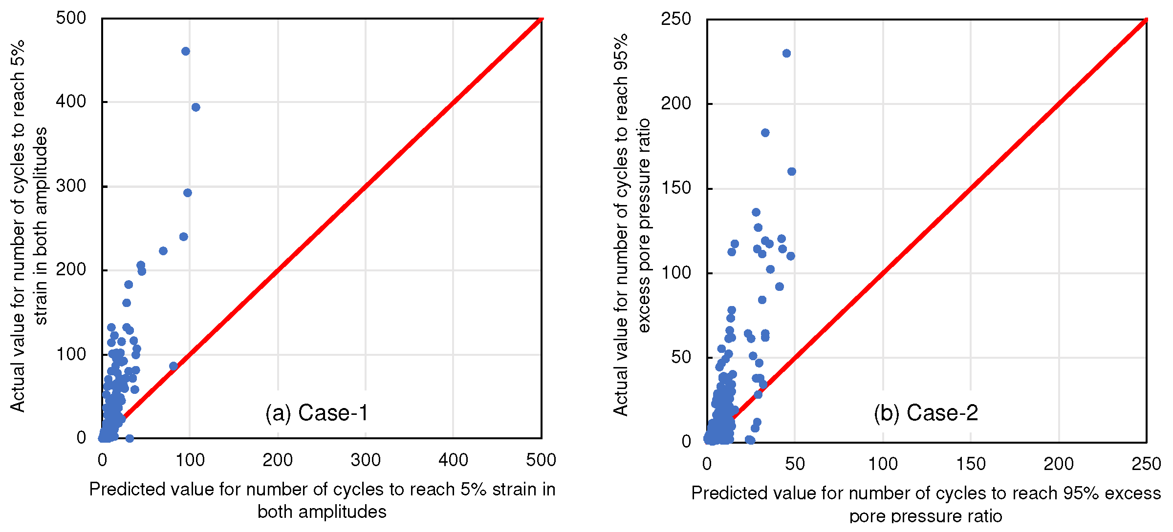
Looking closely at Case-1, shown in Figure 6(a), the Y-axis represents the actual values of the target variable in the training data, while the X-axis represents the values predicted by the ensemble model. In an ideal scenario, the yellow points would align closely along the upward sloping red line, indicating a high degree of accuracy with minimal error between the actual and predicted values. However, in Case-1, the coefficient of determination ( R 2 ) is significantly low at -0.0790. This low accuracy is primarily due to the distribution characteristics of the target variable, "number of cycles to reach 5% strain in both amplitudes," within the training data. Although the range in training data for this goal variable is from 0 to 450, the occurrence of values above 200 is extremely rare. This disproportionate distribution is likely to skew the model′s predictive ability, negatively affecting its accuracy.
In contrast, when examining Case-2, shown in Figure 6(b), the alignment of many yellow points is seen to be closer to the red line, implying improved prediction accuracy compared to Case-1. However, the coefficient of determination ( R 2 ) remains relatively low at 0.0296. This suggests that, similar to Case-1, the intrinsic characteristics of the target variable (number of cycles to reach 95% excess pore pressure ratio) influence the prediction results. It implies that, while the alignment of the data points may visually suggest accuracy, the underlying distribution and nature of the target variable play more significant roles in determining the actual predictive accuracy.
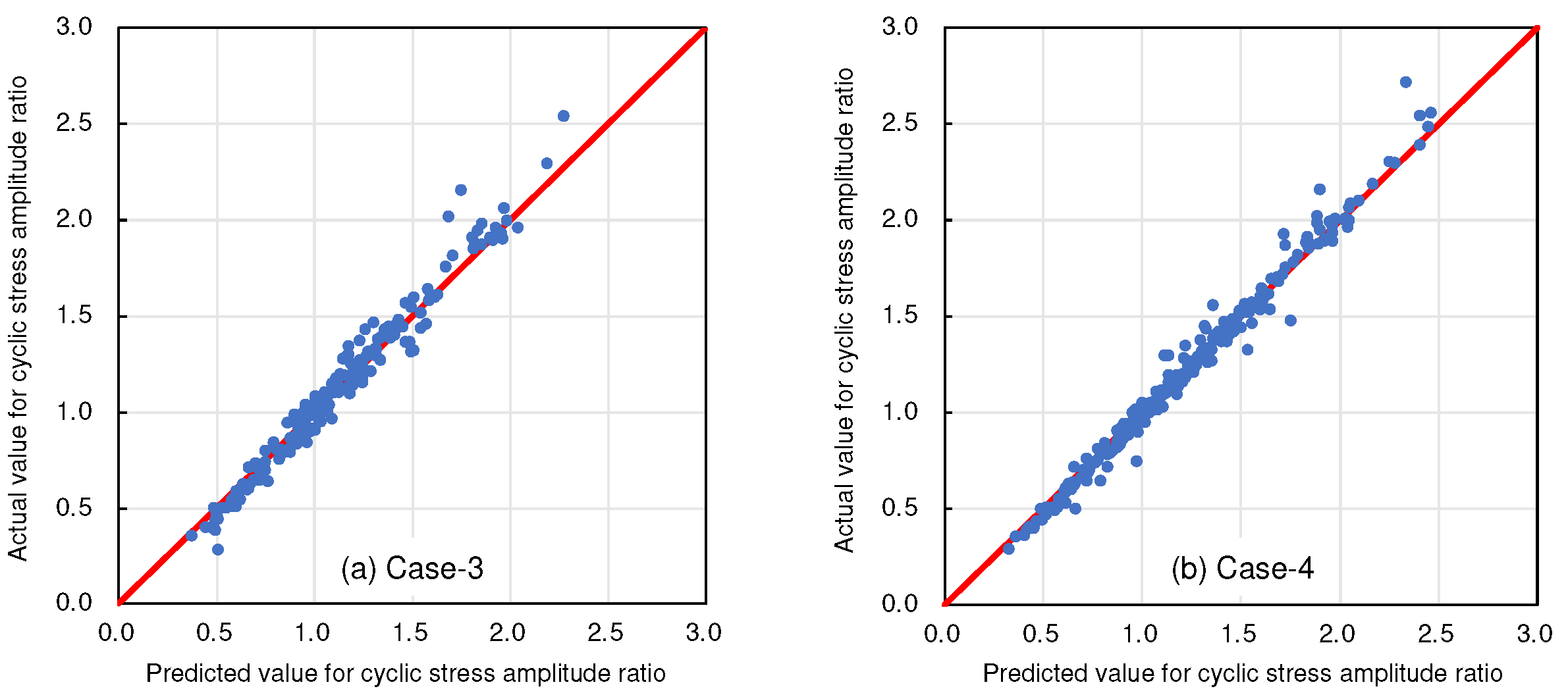
The target variable is changed to "repetitive stress amplitude ratio" in Case-3 and Case-4. This change results in a remarkable agreement between the experimental results and the predicted values. The results of Case-3 and Case-4 are provided in Figure 7, showing a clear and consistent alignment of the yellow points along the red line, visually confirming the high accuracy of the model.
These observations underscore a crucial aspect: the predictive accuracy of the ensemble model developed in this study is strongly influenced by the selection of both explanatory and target variables. The distributional characteristics and inherent nature of these variables are key determinants of the model′s effectiveness.
Furthermore, this analysis highlights the importance of considering skewness and outliers in the training data. The presence of outliers or a skewed distribution can lead to model overfitting or underperformance, as seen in Case-1 and Case-2. In addition, the study highlights the potential limitations of relying solely on graphical representations to assess accuracy. While visual alignment of data points provides an intuitive understanding of model performance, it does not always capture the nuances of the predictive accuracy, especially in cases of non-uniform data distributions.
In addition, the results suggest that preprocessing techniques, such as the normalization or transformation of target variables, could potentially improve model performance. These techniques could help mitigate the problems posed by skewed distributions or outliers, thereby improving the model′s ability to generalize and predict more accurately.
In conclusion, this detailed analysis confirms that the careful selection and preprocessing of explanatory and target variables are critical to improving the predictive accuracy of ensemble models. This insight is invaluable for future studies and applications, emphasizing the need for a thorough understanding of data characteristics and the application of appropriate statistical methods in predictive modeling. The findings from these cases provide a foundation for developing more robust and accurate predictive models in various fields, especially when data distributions are complex or skewed.

4.2. Selecting Explanatory Variables

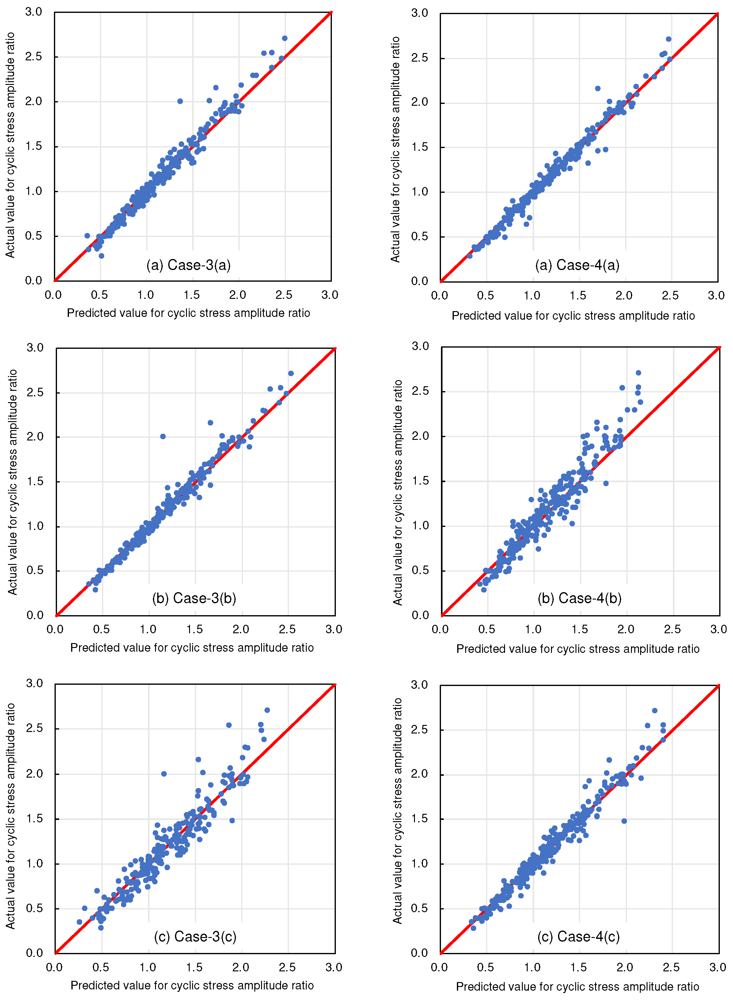
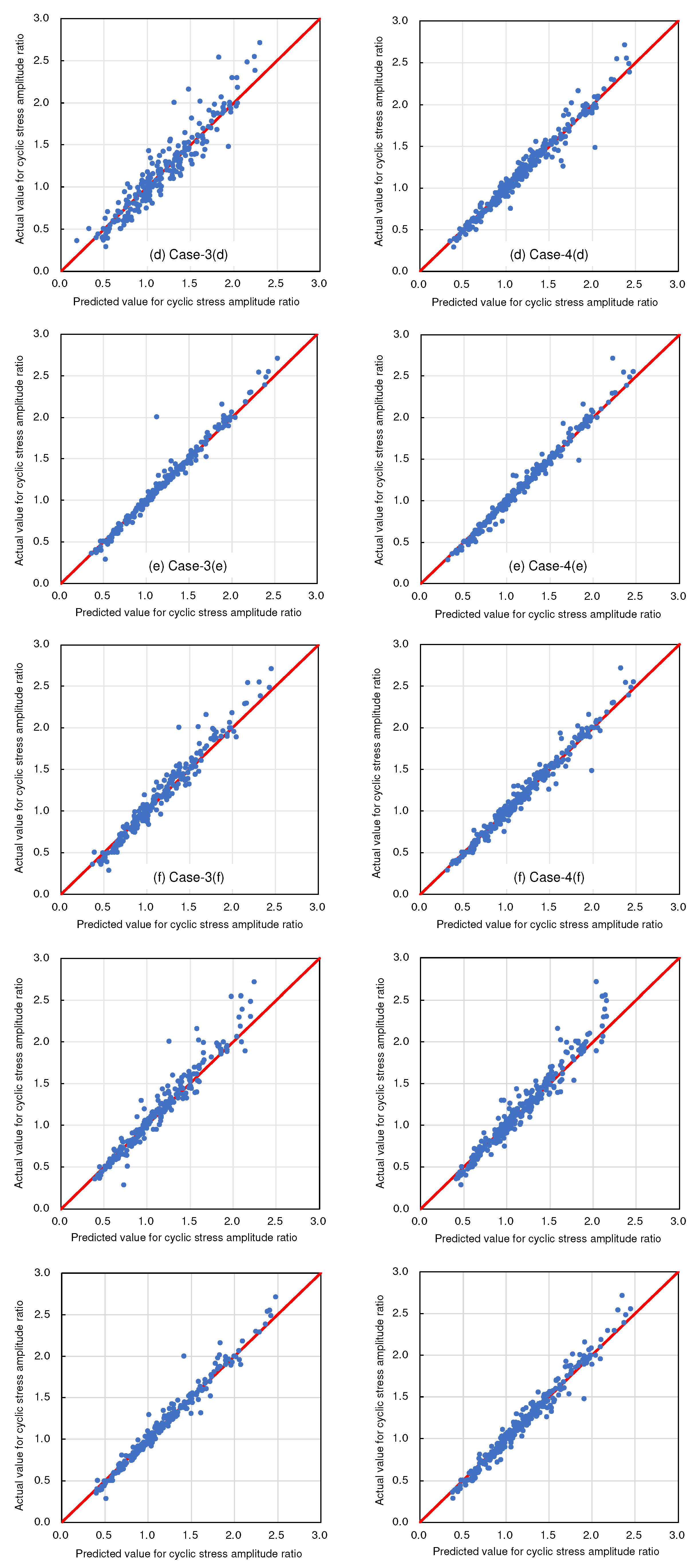
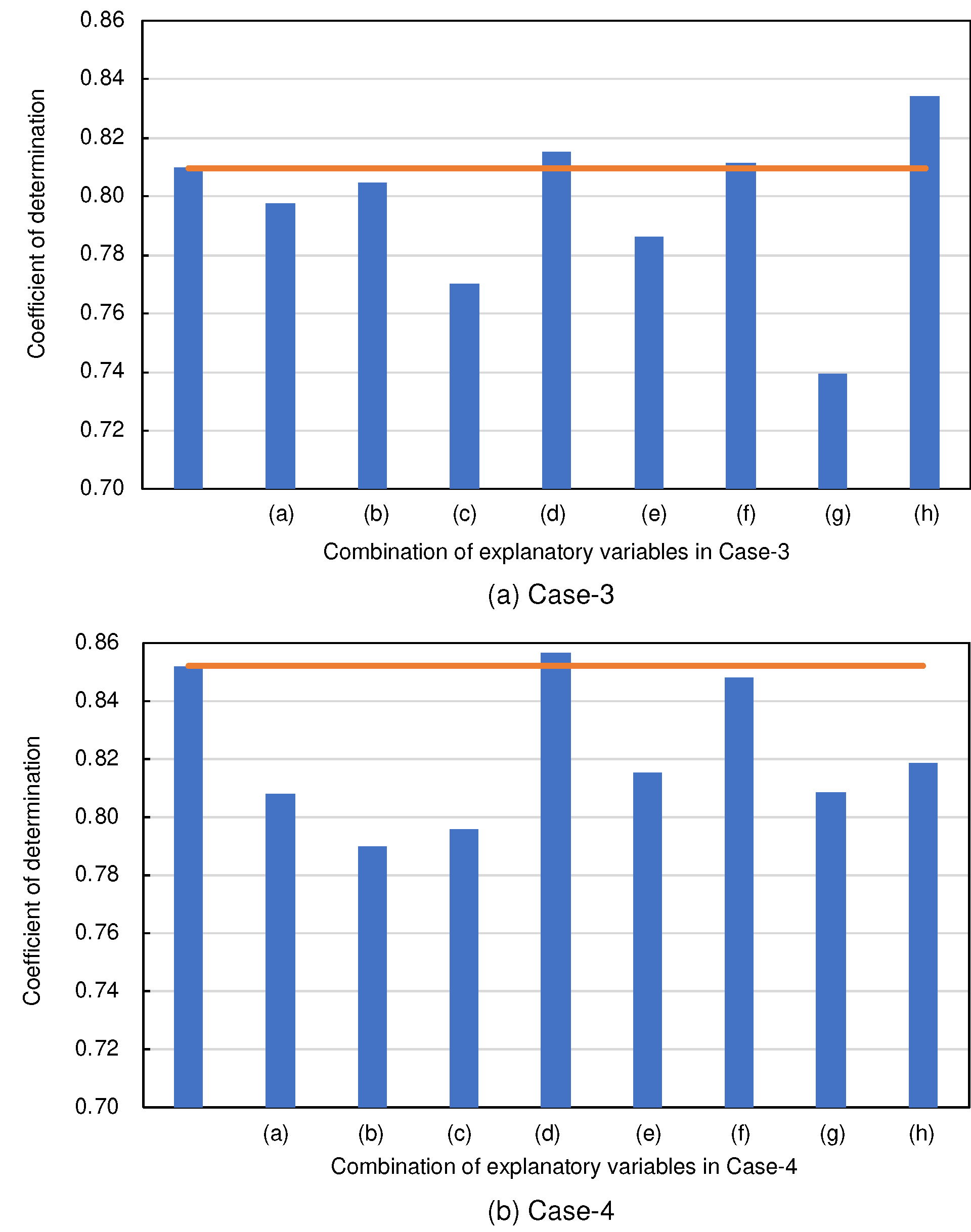
As shown in Table 4, there are eight types of explanatory variables in Case-3 and Case-4, each of which was predicted nine times. The first time, all eight explanatory variables were used simultaneously, namely, Case-3 and Case-4, and their results are shown in Figure 7. The second time, the remaining explanatory variables were used, except dry density, namely, Case-3(a) and Case-4(a), and their results are shown in Figure 8(a). The third time, the remaining explanatory variables were used, except effective confining pressure, namely, Case-3(b) and Case-4(b), and their results are shown in Figure 8(b). The fourth time, the remaining explanatory variables were used, except the fine particle content, namely, Case-3(c) and Case-4(c), and their results are shown in Figure 8(c). The fifth time, the remaining explanatory variables were used, except unconfined compressive strength, namely, Case-3(d) and Case-4(d), and their results are shown in Figure 8(d). The sixth time, the remaining explanatory variables were used, except the silica gel concentration of the injected chemical solution, namely, Case-3(e) and Case-4(e), and their results are shown in Figure 8(e). The seventh time, the remaining explanatory variables were used, except the increase in silica content, namely, Case-3(f) and Case-4(f), and their results are shown in Figure 8(f). The eighth time, the remaining explanatory variables were used, except the number of cycles to reach 5% strain in both amplitudes, namely Case-3(g) and Case-4(g), and their results are shown in Figure 8(g). The ninth time, the remaining explanatory variables were used, except the number of cycles to reach 95% excess pore pressure ratio, namely, Case-3(h) and Case-4(h), and their results are shown in Figure 8(h). These approaches were taken to assess the individual impact of each explanatory variable on the predictive accuracy of the model.
To visualize these effects, Figure 9(a) presents a comprehensive comparison of the coefficients of determination ( R 2 ) for Case-3 and Cases-3(a) to (h), highlighting the changes in the coefficient of determination ( R 2 ) with the inclusion or exclusion of specific variables. Similarly, Figure 9(b) illustrates these comparisons for Case-4 and Cases-4(a) to (h), providing a clear visual representation of the differences between the two cases.
A notable observation from these figures is that Case-4 and Cases-4(a) to (h) consistently showed higher coefficients of determination ( R 2 ) compared to Case-3 and Cases-3(a) to (h). This improvement is primarily due to the increased number and variety of data points used in Case-4 and Cases-4(a) to (h), which improves the model′s ability to generalize and accurately predict outcomes. Additionally, an interesting trend observed in both cases is the increase in the coefficient of determination ( R 2 ) (greater than 0.8) when uniaxial compressive strength is excluded from the training data. This finding suggests that the training data, derived from tests on the same type of sandy soil, provided a consistent and less variable data set, especially in terms of uniaxial compressive strength.
However, it is important to note that uniaxial compressive strength is a critical parameter that reflects the strength characteristics of the local sandy soil. Given its importance, its exclusion raises questions about the potential impact on the predictive accuracy when applied to test results from other sites with different soil characteristics. Therefore, while the current study suggests its lesser significance in the context of the dataset used, further investigation is needed to validate this finding across different soil types and conditions.
In addition, when all the explanatory variables were used in the prediction model, Case-4 showed a coefficient of determination ( R 2 ) of 0.85. This high value indicates a remarkable level of accuracy and reliability in the predictions. It suggests that integrating ensemble learning methods into the analysis can significantly improve the model′s ability to predict the liquefaction resistance in cyclic undrained triaxial tests with high accuracy.
In conclusion, the analysis in Case-4 underscores the importance of selecting appropriate explanatory variables and the potential impact of each on the accuracy of the predictive model. It also highlights the value of ensemble learning methods in improving predictive capabilities, especially in complex geotechnical scenarios such as liquefaction resistance prediction. The results of this study provide a solid foundation for future studies and practical applications in the field of geotechnical engineering.

5. Conclusions

In this study, the primary objective was to evaluate the liquefaction resistance of solution-type chemical sandy soil amendments using a novel approach. By utilizing existing experimental databases and artificial intelligence (AI), we sought to achieve accurate predictions without the need to conduct physical experiments. This methodology focused on analyzing data from 20 loading cycles of cyclic undrained triaxial tests and evaluating the impact of various explanatory variables, leading to an investigation of the optimal combinations of these variables for making predictions.
The results of this study are summarized as follows:
(1)
For the development of a predictive model, it is highly recommended to designate the liquefaction resistance ratio as a dependent variable and the other parameters as explanatory variables. This approach allows a more focused analysis and provides more reliable predictions of the soil behavior under liquefaction conditions.
(2)
The exploration of combinations of explanatory variables revealed that using all available variables tends to produce a more stable coefficient of determination ( R 2 ). This stability is critical to the reliability of the model, especially in applications where precision is paramount.
(3)
Including the liquefaction resistance ratio in the training data set significantly increases the predictive accuracy of the model. This finding underscores the importance of this particular variable in understanding and predicting the behavior of chemically enhanced sandy soils under stress.
(4)
The results of using AI for making predictions highlight the potential of accurately predicting liquefaction resistance using historical data. This approach not only saves time and resources, but also opens new avenues for studies in soil mechanics and geotechnical engineering.
(5)
In addition, this study aimed to validate the effectiveness of the solution-type chemical improvement of sandy soils against liquefaction through AI-based analysis of existing data from cyclic undrained triaxial tests. The results of this study confirmed that high-precision predictions are achievable using the explanatory variables listed in Table 1. In particular, excluding uniaxial compressive strength as an explanatory variable resulted in the highest accuracy, followed closely by scenarios using all explanatory variables. This suggests a nuanced relationship between the variables and their predictive power that warrants further investigation.
Looking ahead, several challenges and opportunities emerge. A key area for future study is to expand the training dataset to include test results from multiple sites. This would improve the generalizability and accuracy of the model and provide a more comprehensive understanding of soil behavior under different geological conditions. In addition, the role of uniaxial compressive strength as an explanatory variable merits further investigation. Its inclusion or exclusion from the model has significant implications for predictive accuracy, suggesting a complex interplay with other variables.
Another future direction is to explore more advanced AI techniques and algorithms. The potential of machine learning and deep learning for improving the predictive models for soil liquefaction resistance is vast and largely untapped. These advanced methods could uncover deeper insights into soil behavior and provide more robust predictive tools for geotechnical engineers.
In conclusion, this study represents a significant step forward in the application of AI for predicting soil liquefaction resistance. It not only demonstrates the feasibility of using AI for such predictions, but also sets the stage for more sophisticated analyses and applications in the field of geotechnical engineering. The integration of AI with traditional soil mechanics offers a promising avenue for future studies, with the potential to revolutionize the way in which soil improvement and liquefaction resistance analysis are approached.

Author Contributions

Conceptualization, S.I. and T.M.; methodology, S.I.; software, Y.C.; validation, K.N. and S.I.; formal analysis, Y.C. and K.N.; investigation, T.M.; resources, T.M.; data curation, Y.C. and K.N; writing—original draft preparation, Y.C.; writing—review and editing, S.I.; visualization, S.I.; supervision, S.I.; project administration, S.I.; funding acquisition, T.M. and S.I. All authors have read and agreed to the published version of the manuscript.

Funding

This research received no external funding.

Data Availability Statement

The authors declare no conflicts of interest.

Conflicts of Interest

The authors declare no conflicts of interest.

References

  1. Kuribayashi, E.; Tatsuoka, F. Brief review of liquefaction during earthquakes in Japan. Soils and Foundations 1975, 15, 81–92. [Google Scholar] [CrossRef]
  2. Huang, Y.; Yu, M. Review of soil liquefaction characteristics during major earthquakes of the twenty-first century. Natural Hazards 2013, 65, 2375–2384. [Google Scholar] [CrossRef]
  3. Hasheminezhad, A.; Bahadori, H. Three dimensional finite difference simulation of liquefaction phenomenon. International Journal of Geotechnical Engineering 2019, 15, 245–251. [Google Scholar] [CrossRef]
  4. Nakao, K.; Inazumi, S.; Takahashi, T.; Nontananandh, S. Numerical simulation of the liquefaction phenomenon by MPSM-DEM coupled CAES. Sustainability 2022, 14, 7517. [Google Scholar] [CrossRef]
  5. Lo, R.C.; Wang, Y. Lessons learned from recent earthquakes-geoscience and geotechnical perspectives. Advances in Geotechnical Earthquake Engineering-Soil Liquefaction and Seismic Safety of Dams and Monuments. 2012, 1–42. [Google Scholar] [CrossRef]
  6. Hazout, L.; Zitouni, Z.E.A.; Belkhatir, M.; Schanz, T. Evaluation of static liquefaction characteristics of saturated loose sand through the mean grain size and extreme grain sizes. Geotechnical and Geological Engineering 2017, 35, 2079–2105. [Google Scholar] [CrossRef]
  7. Bao, X.; Ye, B.; Ye, G.; Zhang, F. Co-seismic and post-seismic behavior of a wall type breakwater on a natural ground composed of liquefiable layer. Nat Hazards 2016, 83, 1799–1819. [Google Scholar] [CrossRef]
  8. Bao, X.; Jin, Z.; Cui, H.; Chen, X.; Xie, X. Soil liquefaction mitigation in geotechnical engineering: An overview of recently developed methods. Soil Dynamics and Earthquake Engineering 2019, 120, 273–291. [Google Scholar] [CrossRef]
  9. Gallagher, P.M.; Pamuk, A.; Abdoun, T. Stabilization of liquefiable soils using colloidal silica grout. Journal of Materials in Civil Engineering 2007, 19, 33–40. [Google Scholar] [CrossRef]
  10. Sayehvand, S.; Kalantari, B. Use of grouting method to improve soil stability against liquefaction -A review. Electronic Journal of Geotechnical Engineering 2012, 17, 1559–1566. [Google Scholar]
  11. Verma, H.; Ray, A.; Rai, R.; Gupta, T.; Mehta, N. Ground improvement using chemical methods: A review. Heliyon 2021, 7, e07678. [Google Scholar] [CrossRef]
  12. Yoon, J.C.; Su, S.W.; Kim, J.M. Method for prevention of liquefaction caused by earthquakes using grouting applicable to existing structures. Applied Sciences 2023, 13, 1871. [Google Scholar] [CrossRef]
  13. Motohashi, T.; Sasahara, S.; Inazumi, S. Strength assessment of water-glass sand mixtures. Gels 2023, 9, 850. [Google Scholar] [CrossRef]
  14. Yoshimi, Y.; Tanaka, K.; Tokimatsu, K. Liquefaction resistance of a partially saturated sand. Soils and Foundations 1989, 29, 157–162. [Google Scholar] [CrossRef]
  15. Mele, L.; Flora, A. On the prediction of liquefaction resistance of unsaturated sands. Soil Dynamics and Earthquake Engineering 2019, 125, 105689. [Google Scholar] [CrossRef]
  16. Park, S.S.; Nong, Z.Z.; Woo, S.W. Liquefaction resistance of Pohang sand. Earthquake Geotechnical Engineering for Protection and Development of Environment and Constructions 2019, 4359–4365. [Google Scholar]
  17. Khashila, M.; Hussien, M.N.; Karray, M.; Chekired, M. Liquefaction resistance from cyclic simple and triaxial shearing: a comparative study. Acta Geotechnica 2021, 16, 1735–1753. [Google Scholar] [CrossRef]
  18. Ni, X.Q.; Zhang, Z.; Ye, B.; Zhang, S. Unique relation between pore water pressure generated at the first loading cycle and liquefaction resistance. Engineering Geology 2022, 296, 106476. [Google Scholar] [CrossRef]
  19. Toyota, H.; Takada, S. Variation of liquefaction strength induced by monotonic and cyclic loading histories. Journal of Geotechnical and Geoenvironmental Engineering 2017, 143, 04016120. [Google Scholar] [CrossRef]
  20. Zhang, J.; Yang, Z.; Yang, Q.; Yang, G.; Li, G.; Liu, J. Liquefaction behavior of fiber-reinforced sand based on cyclic triaxial tests. Geosynthetics International 2021, 28, 316–326. [Google Scholar] [CrossRef]
  21. Khashila, M.; Hussien, M.N.; Karray, M.; Chekired, M. Liquefaction resistance from cyclic simple and triaxial shearing: a comparative study. Acta Geotechnica 2021, 16, 1735–1753. [Google Scholar] [CrossRef]
  22. Nong, Z.Z.; Park, S.S.; Lee, D.E. Comparison of sand liquefaction in cyclic triaxial and simple shear tests. Soils and Foundations 2021, 61, 1071–1085. [Google Scholar] [CrossRef]
  23. Nong, Z.Z.; Park, S.S.; Jeong, S.W.; Lee, D.E. Effect of cyclic loading frequency on liquefaction prediction of sand. Applied Sciences 2021, 10, 4502. [Google Scholar] [CrossRef]
  24. Arpit, J.; Mittal, S.; Shukla, S.K. Liquefaction proneness of stratified sand-silt layers based on cyclic triaxial tests. Journal of Rock Mechanics and Geotechnical Engineering 2023, 15, 1826–1845. [Google Scholar] [CrossRef]
  25. Hyodo, M.; Yasuhara, K.; Hirao, K. Prediction of clay behaviour in undrained and partially drained cyclic triaxial tests. Soils and Foundations 1992, 32, 117–127. [Google Scholar] [CrossRef]
  26. Gu, C.; Wang, J.; Cai, Y.; Yang, Z.; Gao, Y. Undrained cyclic triaxial behavior of saturated clays under variable confining pressure. Soil Dynamics and Earthquake Engineering 2012, 40, 118–128. [Google Scholar] [CrossRef]
  27. Ghayoomi, M.; Suprunenko, G.; Mirshekari, M. Cyclic triaxial test to measure strain-dependent shear modulus of unsaturated sand. International Journal of Geomechanics 2017, 17, 04017043. [Google Scholar] [CrossRef]
  28. Dong, X.; Yu, Z.; Cao, W.; Shi, Y.; Ma, Q. A survey on ensemble learning. Frontiers of Computer Science 2020, 14, 241–258. [Google Scholar] [CrossRef]
  29. Chongzhi, W.; Lin, W.; Zhang, W. Assessment of undrained shear strength using ensemble learning based on Bayesian hyperparameter optimization. Modeling in Geotechnical Engineering 2021, 309–326. [Google Scholar] [CrossRef]
  30. Wang, Z.Z.; Hu, Y.; Guo, X.; He, X.; Kek, H.Y.; Ku, T.; Goh, S.H.; Leung, C.F. Predicting geological interfaces using stacking ensemble learning with multi-scale features. Canadian Geotechnical Journal 2023, 60, 7. [Google Scholar] [CrossRef]
  31. Shahin, M.A. Artificial intelligence in geotechnical engineering: applications, modeling aspects, and future directions. Metaheuristics in Water, Geotechnical and Transport Engineering 2013, 169–204. [Google Scholar]
  32. Jong, S.C.; Ong, D.E.L.; Oh, E. State-of-the-art review of geotechnical-driven artificial intelligence techniques in underground soil-structure interaction. Tunnelling and Underground Space Technology 2021, 113, 103946. [Google Scholar] [CrossRef]
  33. Baghbani, A.; Choudhury, T.; Costa, S.; Reiner, J. Application of artificial intelligence in geotechnical engineering: A state-of-the-art review. Earth-Science Reviews 2022, 228, 103991. [Google Scholar] [CrossRef]
  34. Sharma, S.; Ahmed, S.; Naseem, M.; Alnumay, W.S.; Singh, S.; Cho, G.H. A survey on applications of artificial intelligence for pre-parametric project cost and soil shear-strength estimation in construction and geotechnical engineering. Sensors 2021, 21, 463. [Google Scholar] [CrossRef]
  35. Huang, Y.; Wen, Z. Recent developments of soil improvement methods for seismic liquefaction mitigation. Natural Hazards 2015, 76, 1927–1938. [Google Scholar] [CrossRef]
  36. Mele, L.; Flora, A. On the prediction of liquefaction resistance of unsaturated sands. Soil Dynamics and Earthquake Engineering 2019, 125, 105689. [Google Scholar] [CrossRef]
  37. Fahim, A.K.F.; Rahman, M.Z.; Hossain, M.S.; Kamal, A.M. Liquefaction resistance evaluation of soils using artificial neural network for Dhaka City, Bangladesh. Natural Hazards 2022, 113, 933–963. [Google Scholar] [CrossRef]
  38. Kotsiantis, S.B.; Zaharakis, I.D.; Pintelas, P.E. Machine learning: a review of classification and combining techniques. Artificial Intelligence Review 2006, 26, 159–190. [Google Scholar] [CrossRef]
  39. Pólvora, A.; Nascimento, S.; Lourenço, J.S.; Scapolo, F. Blockchain for industrial transformations: A forward-looking approach with multi-stakeholder engagement for policy advice. Technological Forecasting and Social Change 2020, 157, 120091. [Google Scholar] [CrossRef]
  40. Tuttle, M.P.; Hartleb, R.; Wolf, L.; Mayne, P.W. Paleoliquefaction studies and the evaluation of seismic hazard. Geosciences 2019, 9, 311. [Google Scholar] [CrossRef]
  41. Dhakal, R.; Cubrinovski, M. Geotechnical characterization and liquefaction evaluation of gravelly reclamations and hydraulic fills (Port of Wellington, New Zealand). Soils and Foundations 2020, 60, 1507–1531. [Google Scholar] [CrossRef]
  42. Yang, M.; Taiebat, M.; Radjaï, F. Liquefaction of granular materials in constant-volume cyclic shearing: Transition between solid-like and fluid-like states. Computers and Geotechnics 2022, 148, 104800. [Google Scholar] [CrossRef]
  43. Mitchell, J.K. Mitigation of liquefaction potential of silty sands. From Research to Practice in Geotechnical Engineering 2008, 433–451. [Google Scholar] [CrossRef]
  44. Kramer, S.L. and Mitchell, R. A. Ground motion intensity measures for liquefaction hazard evaluation. Earthquake Spectra 2006, 22, 413–438. [Google Scholar] [CrossRef]
  45. Zhou, Z.H. Ensemble Methods: Foundations and Algorithms (Chapman & Hall/CRC Machine Learning & Pattern Recognition). CRC Press 2012. [Google Scholar]
  46. Gurney, K. An Introduction to Neural Networks 1st Edition. CRC Press 1997. [Google Scholar]
  47. Zhao, Z.; Chow, T.L.; Rees, H.W.; Yang, Q.; Xing, Z. and Meng, F. R. Predict soil texture distributions using an artificial neural network model. Computers and electronics in agriculture 2009, 65, 36–48. [Google Scholar] [CrossRef]
  48. Zhong, L.; Guo, X.; Xu, Z.; Ding, M. Soil properties: Their prediction and feature extraction from the LUCAS spectral library using deep convolutional neural networks. Geoderma 2021, 402, 115366. [Google Scholar] [CrossRef]
  49. Pham, B.T.; Nguyen, M.D.; Ly, H.B.; Pham, T.A.; Hoang, V.; Le, V.H.; Le, T.T.; Nguyen, H.Q.; Bui, G.L. Development of artificial neural networks for prediction of compression coefficient of soft soil. In Proceedings of the 5th International Conference on Geotechnics, Civil Engineering Works and Structures; 2020; pp. 1167–1172. [Google Scholar] [CrossRef]
  50. Chakraborty, D.; Elhegazy, H.; Elzarka, H.; Gutierrez, L. A novel construction cost prediction model using hybrid natural and light gradient boosting. Advanced Engineering Informatics 2020, 46, 101201. [Google Scholar] [CrossRef]
  51. Lee, S.; Vo, T.P.; Thai, H.T.; Lee, J.; Patel, V. Strength prediction of concrete-filled steel tubular columns using Categorical Gradient Boosting algorithm. Engineering Structures 2021, 238, 112109. [Google Scholar] [CrossRef]
  52. Guo, R.; Fu, D. and Sollazzo, G. An ensemble learning model for asphalt pavement performance prediction based on gradient boosting decision tree. International Journal of Pavement Engineering 2022, 23, 3633–3646. [Google Scholar] [CrossRef]
  53. Nakagawa, S.; Johnson, P.C.D.; Schielzeth, H. The coefficient of determination R2 and intra-class correlation coefficient from generalized linear mixed-effects models revisited and expanded. Journal of the Royal Society Interface 2017, 14, 1–11. [Google Scholar] [CrossRef]
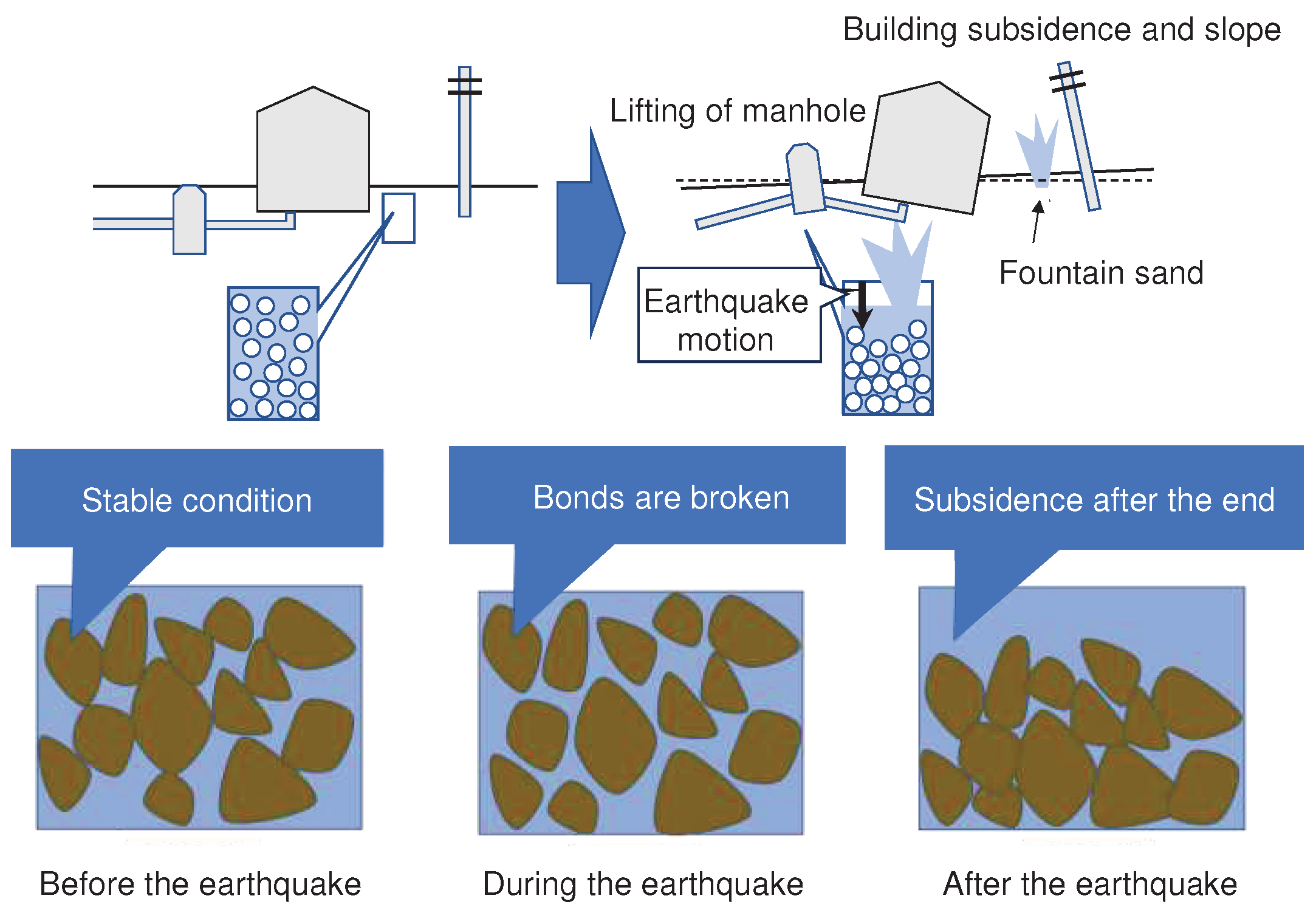
Figure 1. General principle of liquefaction phenomenon.
Preprints 97385 g001
Figure 2. Typical appearance of cyclic undrained triaxial test.
Preprints 97385 g002
Figure 3. Liquefaction intensity curves obtained from cyclic undrained triaxial tests.
Preprints 97385 g003
Figure 4. Schematic prediction flow of neural network.
Preprints 97385 g004
Figure 5. Schematic prediction flow of proposed ensemble model.
Preprints 97385 g005
Figure 6. Degrees of deviation between predicted and measured values in Case-1 and Case-2.
Preprints 97385 g006
Figure 7. Degrees of deviation between predicted and measured values in Case-3 and Case-4.
Preprints 97385 g007
Figure 8. Degrees of deviation between predicted and measured values in Cases-3(a) to (h) and Cases-4(a) to (h).
Preprints 97385 g008aPreprints 97385 g008b
Figure 8. Comparisons of accuracy for predictions in Case-3, Cases-3(a) to (h), Case-4 and Cases-4(a) to (h).
Preprints 97385 g009
Table 1. Variable elements related to cyclic undrained triaxial test employed in training data.
Category Variable elements
Condition parameters for specimens of chemically improved sandy soils Dry density (g/cm3)
Fine particle content (%)
Effective confining pressure (kN/m2)
Unconfined compressive strength (kN/m2)
Silica gel concentration of injected chemical solution (%)
Increase in silica content (mg/g)
Results obtained by cyclic undrained triaxial test Number of cycles to reach 5% strain in both amplitudes
Number of cycles to reach 95% excess pore pressure ratio
Cyclic stress amplitude ratio
Liquefaction resistance ratio*
*It refers to the cyclic amplitude stress ratio when the axial strain amplitude reaches 5% or the excess pore water pressure ratio reaches 95% and the number of cyclic loads is 20.
Table 2. Explanatory and target variables employed for each prediction case.
Case Explanatory variables Target variables
Case-1 Variable elements shown in Table 1 excluding the liquefaction resistance ratio and the target variable Number of cycles to reach 5% strain in both amplitudes
Case-2 Variable elements shown in Table 1 excluding the liquefaction resistance ratio and the target variable Number of cycles to reach 95% excess pore pressure ratio
Case-3 Variable elements shown in Table 1 excluding the liquefaction resistance ratio and the target variable Cyclic stress amplitude ratio
Case-4 Variable elements shown in Table 1 excluding the target variable Cyclic stress amplitude ratio
Table 3. Example of employed training data (data on 2 out of 272 specimens were extracted).
Variable Variable elements Data for 2 of 272 specimens
Explanatory variables Dry density (g/cm3) 1.684 1.484
Effective confining pressure (kN/m2) 90 165
Fine particle content (%) 14.8 11.4
Unconfined compressive strength (kN/m2) 539 483
Silica gel concentration of injected chemical solution (%) 12 12
Increase in silica content (mg/g) 11.62 7.79
Number of cycles to reach 5% strain in both amplitudes 18 6.5
Number of cycles to reach 95% excess pore pressure ratio 37 38.4
Target variable Repetitive stress amplitude ratio
Table 3. Example of employed training data (data on 2 out of 272 specimens were extracted).
Case-3 and Case-4
Explanatory variables (a) (b) (c) (d) (e) (f) (g) (h)
Dry density (g/cm3) x
Effective confining pressure (kN/m2) x
Fine particle content (%) x
Unconfined compressive strength (kN/m2) x
Silica gel concentration of injected chemical solution (%) x
Increase in silica content (mg/g) x
Number of cycles to reach 5% strain in both amplitudes x
Number of cycles to reach 95% excess pore pressure ratio x
Disclaimer/Publisher’s Note: The statements, opinions and data contained in all publications are solely those of the individual author(s) and contributor(s) and not of MDPI and/or the editor(s). MDPI and/or the editor(s) disclaim responsibility for any injury to people or property resulting from any ideas, methods, instructions or products referred to in the content.
Copyright: This open access article is published under a Creative Commons CC BY 4.0 license, which permit the free download, distribution, and reuse, provided that the author and preprint are cited in any reuse.
Prerpints.org logo

Preprints.org is a free preprint server supported by MDPI in Basel, Switzerland.

Subscribe

© 2024 MDPI (Basel, Switzerland) unless otherwise stated