Towards An Info-Geometric Theory Of The Analysis Of Non-Time Dependent Queueing Systems

Preprint

Article

Towards An Info-Geometric Theory Of The Analysis Of Non-Time Dependent Queueing Systems

Altmetrics

Downloads

100

Views

Comments

Ismail A. Mageed^*

This version is not peer-reviewed

Submitted:

30 January 2024

Posted:

30 January 2024

You are already at the latest version

Alerts

Abstract

Information geometry (IG) seeks to characterize the structure of statistical geodesic models from a differential geometric point of view. By considering families of probability distributions as manifolds with coordinate charts determined by the parameters of each individual model, the tools of differential geometry, such as divergences and metric tensors, provide effective means of studying their characteristics. The research undertaken in this paper presents a novel approach to the modelling study of information geometrics of a queueing system. In this context, the manifold of a stable M/G/1queue is characterised from the viewpoint of IG. The Fisher Information matrix (FIM) as well as the inverse of (FIM), (IFIM) of stable M/G/1 queue manifold are devised. In addition to that, new results that uncovered the significant impact of stability of M/G/1 queue manifold on the existence of (IFIM) are obtained. The Kullback’s divergence (KD), and J-divergence (JD).New result has been devised on the significant impact of both server utilization and squared coefficient of variation of the underlying M/G/1 queue manifold on both (KD) and (KD) are devised. Also, it is revealed that stable M/G/1 QM is developable (i.e., has a zero Gaussian curvature) and has a non-zero Ricci Curvature Tensor (RCT). Novel stability dynamics of M/G/1 queue manifold is revealed by discovering the mutual dual impact between the behaviour of (RCT) and the stability and the instability phases of the underlying M/G/1 queue manifold. Furthermore, a new discovery that presents the significant impact of stability of M/G/1 queue manifold and the continuity of the unique representation between M/G/1 queue manifold and Ricci Curvature Tensor (RCT). The information matrix exponential (IME) is devised. It is also shown that the obtained (IME) is unstable. Also, it is shown that stability of the devised (IME) enforces the instability of M/G/1 queue manifold. Unifying IG with Queueing Theory enables the study of dynamics of queueing system from a novel Riemannian Geometric (RG) point of view, leading to the analysis of the stable M/G/1 queue, based on the Theory of Relativity (TR).Extending the study over two new additional divergence measures, namely and together with a complete illustrative numerical results for all these measures including KD, JD. This links Queueing theory, IG with deep machine learning and metric learning. Furthermore, this reveals the revolutionary approach of queue learning. Full analytic study of Gaussian curvatures subject to both Angular and Monge techniques together with the overall stability dynamics impact on these curvatures. Full analytic study of Einestein Tensor and Stress Energy Tensor together with the overall stability dynamics impact on these curvatures. The inclusion of the definitions of Gaussian and Ricci, Ricci scalar curvatures and Einstein Tensor together with their physical interpretations; The proposed novel approach for the pioneer visualization of queueing systems via computational information geometry. The determination of new important links between classical queueing theory and other mathematical disciplines, such as IG, matrix theory Riemannian geometry and the THEORY OF RELATIVITY by providing for first time i) The full detailed derivations of the Gaussian curvature ii) The Ricci curvature tensor and iii) The full physical as well as the geometric interpretation of these new results. The provision of a novel link between Ricci Curvature (RCT) and the stability analysis of the stable M/G/1 QM. The full investigation of the newly introduced QT-IG unifiers together with the impact of stability/ instability of the underlying M/G/1 QM on them. The full investigation of the newly introduced (QIGU) unifiers together with the impact of stability/ instability of the underlying M/G/1 QM on them.

Keywords:

Subject: Computer Science and Mathematics - Applied Mathematics

1. Introduction

Information geometry (IG) is a field that applies techniques from differential geometry to statistics [1]. It aims to use geometric metrics to provide a new way to describe the probability density function, serving as a coordinate system in statistical manifolds(SMs). A manifold [2]is a mathematical concept that represents a space with certain properties. In this context, a manifold is a finite-dimensional Cartesian space, denoted as

ℝ^{n}

, where

ℝ^{n}

refers to a topological space. It is important to note that although figures can be visualized, they are considered abstract geometric figures rather than concrete representations.

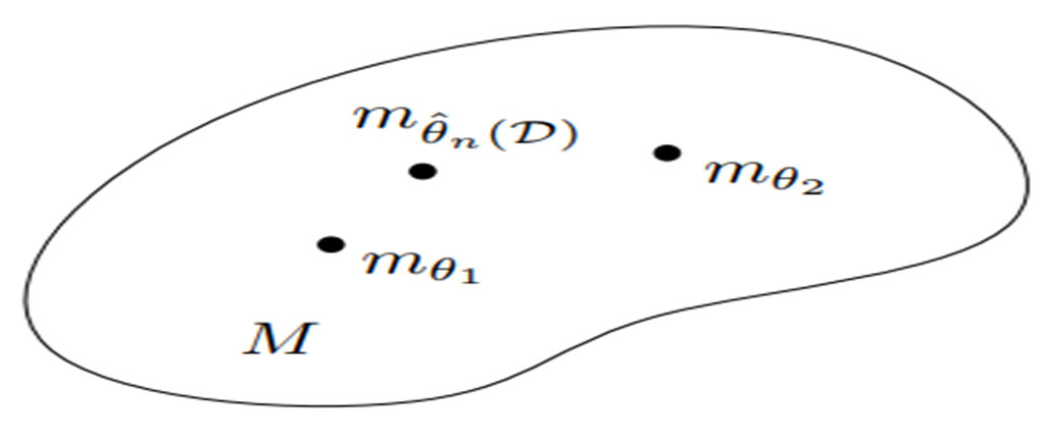
In the given context, IG is highlighted as being significantly important[1,3,4]. Figure 1 illustrates how parameter inference, represented by

\hat{θ}

. Additionally, previous research has explored the geometric structures of exponential distribution families.

One mathematical method for solving systems of linear differential equations is the information matrix exponential (IME). It also has significant applications in the theory of Lie groups, which are mathematical structures that have important implications in various areas of mathematics and physics [5]. Interarrival time distribution (IG) of stable M/D/1 queues was studied by using features of queue length pathways, the article introduced a geometric structure to the set of M/D/1 queues, for a more detailed survey, consult [5]. This strategy connected information matrix theories with IG, opening new insights into queueing theory. According to [3,6], Ricci curvature quantifies the distinction between the standard Euclidean metric (EM) and the Riemannian metric (RM) in the setting of the article. In contrast, the difference in volume between a geodesic ball and a Euclidean ball with the same radius is measured by scalar curvature. Figure 2 depicts the knowledge facilitation of comprehension of the geometric characteristics of spaces and how they deviate from Euclidean geometry (c.f., Figure 2).

[7] states that the exponential of the Fisher Information Matrix (FIM) for the stable M/G/1 queue, a mathematical model used in queueing theory, solves dx/dt $= A x$ . Here, x represents a vector with n dimensions, and A is a nxn matrix. The second extended study by [7] builds upon their previous work [8] and introduces new contributions:
Finding the underlying QM’s KD and JD measures
Proving that FIM of the underlying QM solves: dx/dt $= A x$ .
This current paper is an ultimate extension of both papers, with main deliverables:
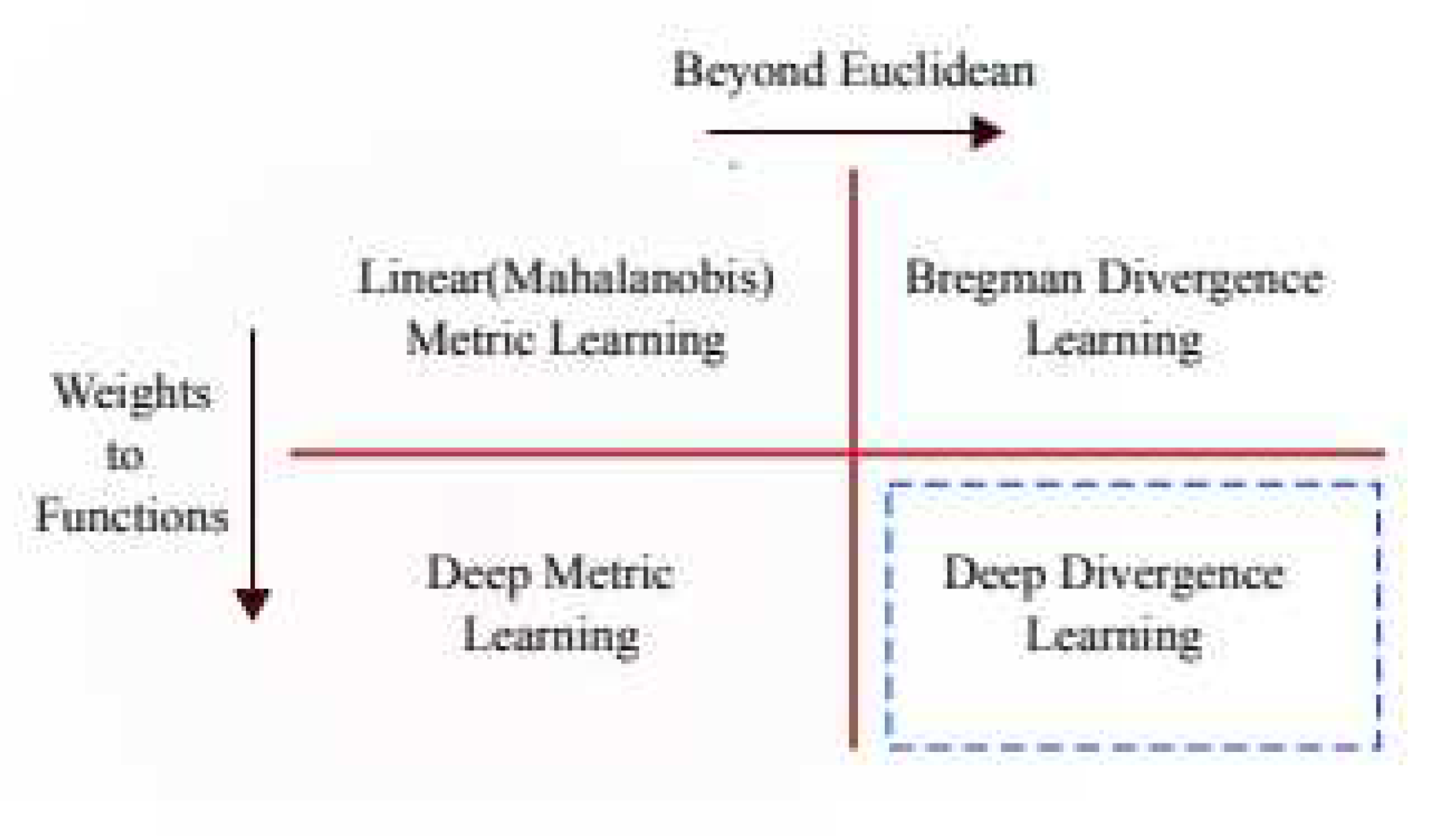
Extending the study over two new additional divergence measures, namely $R é nyi ’ s$ and $s A B ’ s$ together with a complete illustrative numerical result for all these measures including KD, JD. This links Queueing theory, IG with deep machine learning and metric learning. Furthermore, this reveals the revolutionary approach of queue learning.
iv) The solenoidability(incompressibility) of the underlying queueing system is shown. This concept is analogous to the Divergence Theorem[9].
Full analytic study of Gaussian curvatures subject to both Angular and Monge techniques together with the overall stability dynamics impact on these curvatures.
The current paper provides a comprehensive analysis of the Einstein Tensor and Stress Energy Tensor, exploring their relationship with stability dynamics and curvatures. It also introduces the definitions and interpretations of Gaussian and Ricci curvatures, as well as the Einstein Tensor.
Extending the study to include two new divergence measures, Rényi’s and $s A B ’ s$ , along with illustrative numerical results such as KD and JD. This extension connects queueing theory, information geometry, deep machine learning, and metric learning, revealing a novel approach called queue learning.
Additionally, the paper explores the impact of stability dynamics on Gaussian curvatures, provides a comprehensive analysis of Einsteinian and Stress Energy Tensors, and establishes a unified theorem of queueing-theoretic correlations with both special and general relativity.

The road map of this study is: The core definitions for IG are contained in Section 2. In Section 3, FIM and its inverse for the underlying QM are obtained. In Section 4, the α-connection of a stable M/G/1 queue manifold is obtained. In Section 5, the KD and JD [7], Rényi’s, and sAB divergences of a stable M/G/1 QM are computed. In Section 6, methodical arguments are developed demonstrating the developability and non-zero RCT for the underlying queuing manifold system. In addition, a comprehensive examination of the recently announced QT-IG unifiers is presented in Section 6. Section 7 investigates

e^{F I M (M / G / 1)}

and how the underlying QM’s stability impacts FIM’s stability.

In section 8, Ricci scalar,

R, curvature of space time (einestein tensor) ℘, stress energy tensor, Τ

, the corresponding threshold theorems for the underlying curvatures and the dual queueing impact on the existence of the inverse fisher information matrix(IFIM). Section 9 discusses Queueing theoretic impact on the continuity of new devised queueuing-information geometric unifiers (QIGU). Section 10 is entirely devoted to closing remarks combined with next phase of research.

2. Main Definitions

2.1. Main Definition on IG

Definition 2.1 Statistical Manifold (SM) [7]

We denote a statistical manifold, M = {p (x, θ) | θ ϵ Θ}

and

p (x, θ)

as a PDF. Here,

θ = (θ_{1}, θ_{2}, .., θ_{n}) ϵ Θ

\subset ℝ^{n}

Definition 2.2 Potential Function [7]

The potential function

Ψ (θ)

denotes (

- L (x; θ) = - l n (p (x; θ))

) with coordinates only.

Definition 2.3 FIM, namely [

g_{i j}

]

[

g_{i j}

](c.f., [7]) reads as

[g_{i j}] = [\frac{\partial^{2}}{\partial θ^{i} \partial θ^{j}} (Ψ (θ))], i, j = 1, 2, .., n

(2.1)

Definition 2.4 IFIM, namely [

g^{i j}]

(c.f., [7])

[g^{i j}] = ([g_{i j}]))^{- 1} = \frac{a d j [g_{i j}]}{Δ}, Δ = \det [g_{i j}]

(2.2)

The arc length is defined to be:

{(d s)}^{2} = \sum_{i, j = 1}^{n} g_{i j} (d θ^{i}) (d θ^{j})

(2.3)

Definition 2.5

α

-Connection(c.f., [7])

The

α

-connection reads as

Γ_{i j, k}^{(α)} = (\frac{1 - α}{2}) (\partial_{i} \partial_{j} \partial_{k} (Ψ (θ))), \partial_{i} \frac{\partial}{\partial θ_{i}}, α is real

(2.4)

Definition 2.6 Kullback’s Divergence (KD),

K (p, q)

KD, namely

K (p, q)

[7]reads as

K (p, q) = E_{θ_{p}} [l n (\frac{p (x; θ_{p})}{q (x; θ_{q})})]

(2.5)

= \int p (x; θ_{p}) l n (\frac{p (x; θ_{p})}{q (x; θ_{q})}) d x

(2.6)

J-divergence reads as

J (p, q) = l n {(\frac{p (x; θ_{p})}{q (x; θ_{q})})}^{(p (x; θ_{p}) - q (x; θ_{q}))} d x

(2.7)

= K (p, q) + K (q, p)

(2.8)

In this paper, however, we focus on the Rényi divergence [10,11],

D_{R}^{γ} (p | | q) = \frac{1}{(γ - 1)} l n (\sum_{n = 0}^{\infty} {(p (n))}^{γ} {(q (n))}^{1 - γ})

(2.9)

used in Rényi variational inference VI [12].

D_{s, A B}^{γ, η} (p | | q)

[13] reads as:

D_{s, A B}^{γ, η} (p | | q) = \frac{1}{η (η + γ)} l n (\sum_{n = 0}^{\infty} {(p (n))}^{γ + η}) + \frac{1}{γ (η + γ)} l n (\sum_{n = 0}^{\infty} {(q (n))}^{γ + η}) - \frac{1}{γ η} l n (\sum_{n = 0}^{\infty} {(p (n))}^{γ} {(q (n))}^{η})

(2.10)

for

(γ, η) ϵ ℝ^{2}

such that

γ \neq 0, η \neq 0 a n d γ + η \neq 0.

The authors [13] have presented a novel (dis)similarity measure, namely

D_{s, A B}^{γ, η} (p | | q)

(c.f., (2.10)). Moreover, it has been illustrated [13] that

D_{s, A B}^{γ, η} (p | | q)

is potentially robust.

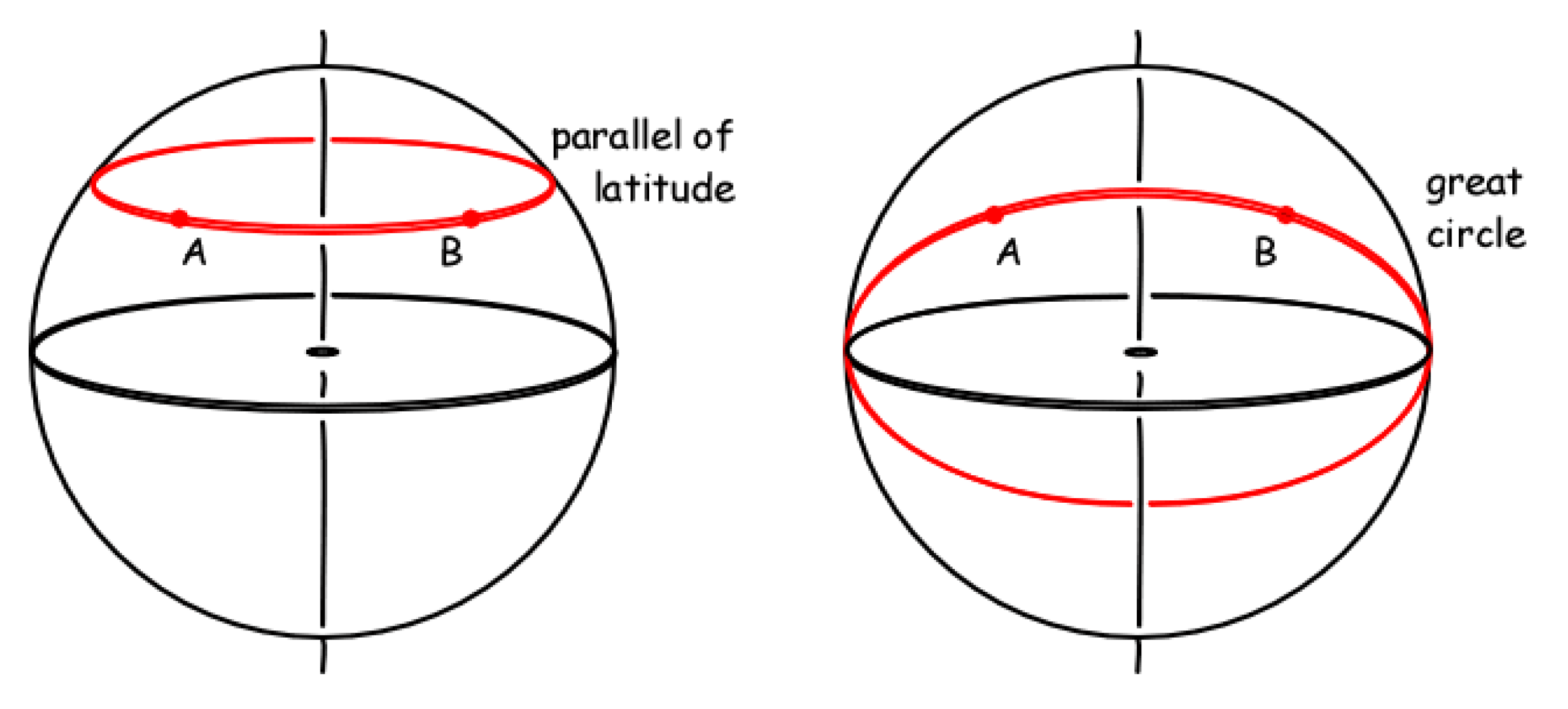
Figure 3. (c.f., [14]).

Definition 2.8

1. The $α - curvature Riemannian$

Tensors, $R_{i j k l}^{(α)}$ [7] reads

$R_{i j k l}^{(α)} = [(\partial_{j} Γ_{i k}^{s (α)} - \partial_{i} Γ_{j k}^{s (α)}) g_{s l} + (Γ_{j t, l}^{(α)} Γ_{i k}^{t (α)} - Γ_{i t, l}^{(α)} Γ_{j k}^{t (α)})], i, j, k, l, s, t = 1, 2, 3, \dots ., n$

(2.11)

where $Γ_{i j}^{k (α)} = Γ_{i j, s}^{(α)} g^{s k}$ , i,j,k,s = 1,2,...,n

2. The $α - Ricci$

curvatures (Ricci Tensors) $R_{i k}^{(α)}$ reads [7]

$R_{i k}^{(α)} = R_{i j k l}^{(α)} g^{j l}, i, j, k, l = 1, 2, 3, \dots ., n$

(2.12)

3.The $α - \sec tional curvatures K_{i j i j}^{(α)}$ reads [7]

$K_{i j i j}^{(α)} = \frac{R_{i j i j}^{(α)}}{(g_{i i}) (g_{j j}) - {(g_{i j})}^{2}}, i, j = 1, 2, \dots, n$

(2.13)

Potentially,

$K^{(α)} = \frac{R_{1212}^{(α)}}{d e t (g_{i j})}$

(2.14)

4. One mathematical object that can be obtained by contacting the Riemannian Tensor is the Ricci Tensor [15]. It measures the curvature of space and is employed in the study of Riemannian manifolds. To obtain the Ricci Tensor, the contraction procedure entails summing a few components of the Riemannian Tensor [7].

5. An oriented Riemannian manifold’s Ricci curvature tensor (RCT) (c.f., [16]) quantifies the difference between a geodesic ball’s volume on the manifold and its volume in Euclidean space. It gives details on the manifold’s curvature and how it differs from flat space. knowledge the geometry and characteristics of curved spaces in connection to Euclidean geometry requires a knowledge of this topic.

6.RCT (c.f., [17]) measures how volumes change over time along geodesic paths on a Riemannian manifold. When the Ricci curvature is positive, it indicates a smaller diameter. This relationship is supported by the Bonnet-Myers theorem, which establishes a connection between the manifold’s positive Ricci curvature and the curvature properties.

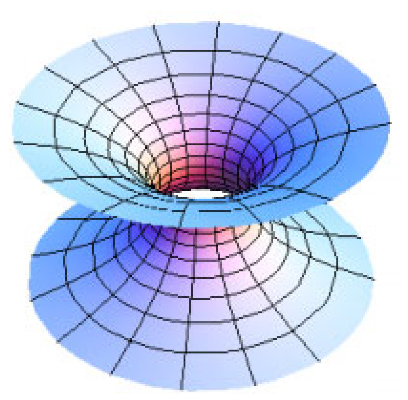
Figure 4. RCT (c.f., [18]).

Definition 2.9

1. Considering the linear system of differential equations

\frac{d x}{d t} = A x

(2.15)

with x is an n-dimensional vector and A is a nxn matrix. It can be shown that (Gunawardena, 2006) the matrix exponential:

e^{A} = \sum_{i = 0}^{\infty} \frac{A^{i}}{i!} = I + A + \frac{A^{2}}{2!} + \dots + \frac{A^{k}}{k!} + ....

(2.16)

is the solution of (2.15).

2. If the characteristic polynomial of A is defined by

Φ (δ) = \det (A - δ I)

(2.17)

The eigen values of A (c.f., [19]) solve:

Φ (δ) = (δ) = 0

(2.18)

such that:

A x = δ x

(2.19)

e^{A}

reads as:

e^{A} = T e^{D} T^{- 1}

(2.20)

where D is the diagonal matrix of eigen values of A, and T is matrix having of the corresponding eigen vectors of A as its columns (c.f., [19]).

Definition 2.10

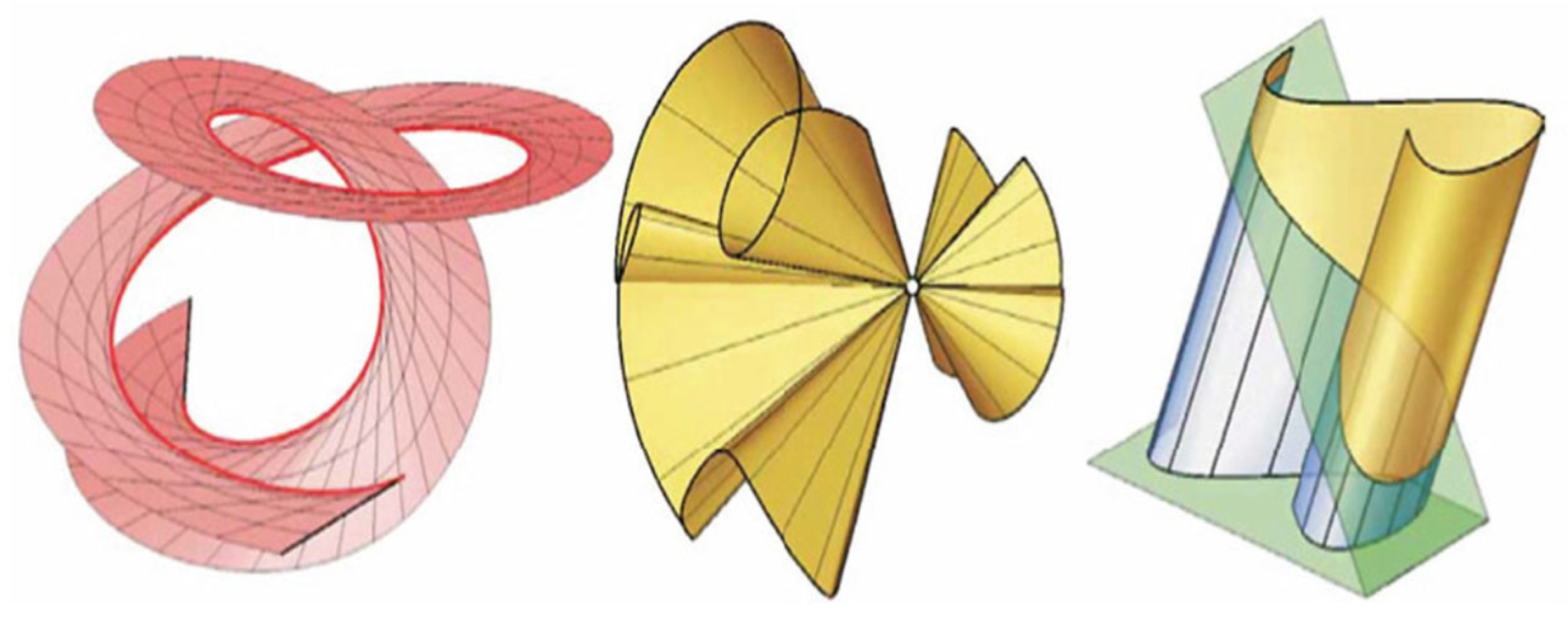
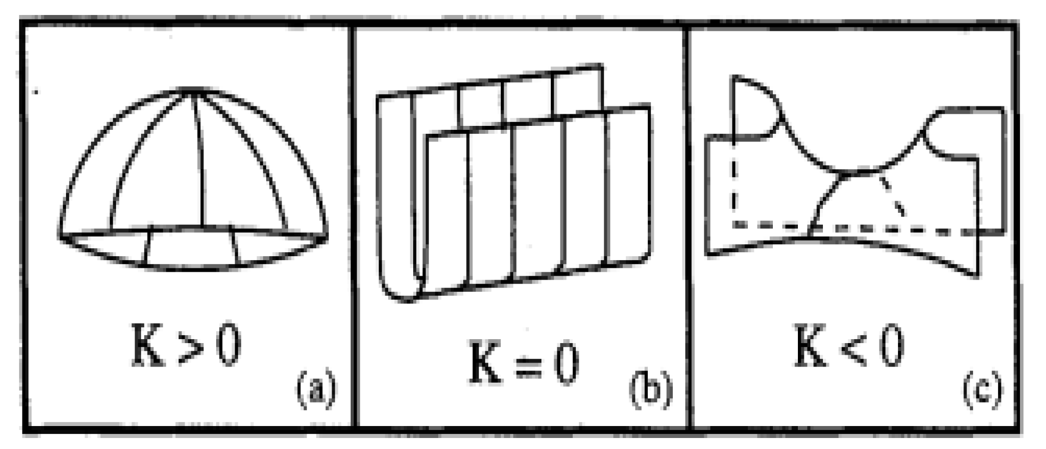
Developable surfaces are a special kind of ruled surfaces, they have a Gaussian curvature equal to 0, and can be mapped onto the plane surface without distortion of curves: any curve from such a surface drawn onto the flat plane remains the same (c.f., [20]).

Figure 5. Three kinds of developable surfaces: Tangential on Figure. 5a (on the left), Conical on Figure 5b (on the centre) and Figure. 5c (on the right), Cylindrical. Note that curves in bold are directrix or base curves and straight lines in bold are directors or generating lines (curves) (c.f., [20]).

2.2. Gaussian and Mean Curvatures, K_Gand H respectively (c.f., [21])

Definition 2.11(Mong Patch Technique)

1.Let

K_{1}

and

K_{2}

be the principal curvatures of a surface patch

δ (u, v) . K_{G}

(

δ)

K_{G} = K_{1} K_{2}

(2.21)

and its Mean Curvature is:

H = \frac{1}{2} (K_{1} + K_{2})

(2.22)

2.For a Mong patch

z = f (x, y), K_{G}

and

H

are given by

K_{G} = \frac{L N - M^{2}}{E G - F^{2}}

(2.23)

and its Mean Curvature is

H = \frac{1}{2} (\frac{L G - 2 M F + N E}{E G - F^{2}})

(2.24)

with

E = {(\frac{\partial f}{\partial x})}^{2}, F = \frac{\partial f}{\partial x \partial y}, G = {(\frac{\partial f}{\partial y})}^{2}, L = \frac{\partial^{2} f}{\partial x^{2}}, M = \frac{\partial f}{\partial x y}, N = \frac{\partial^{2} f}{\partial y^{2}}

Classification of Surface Points

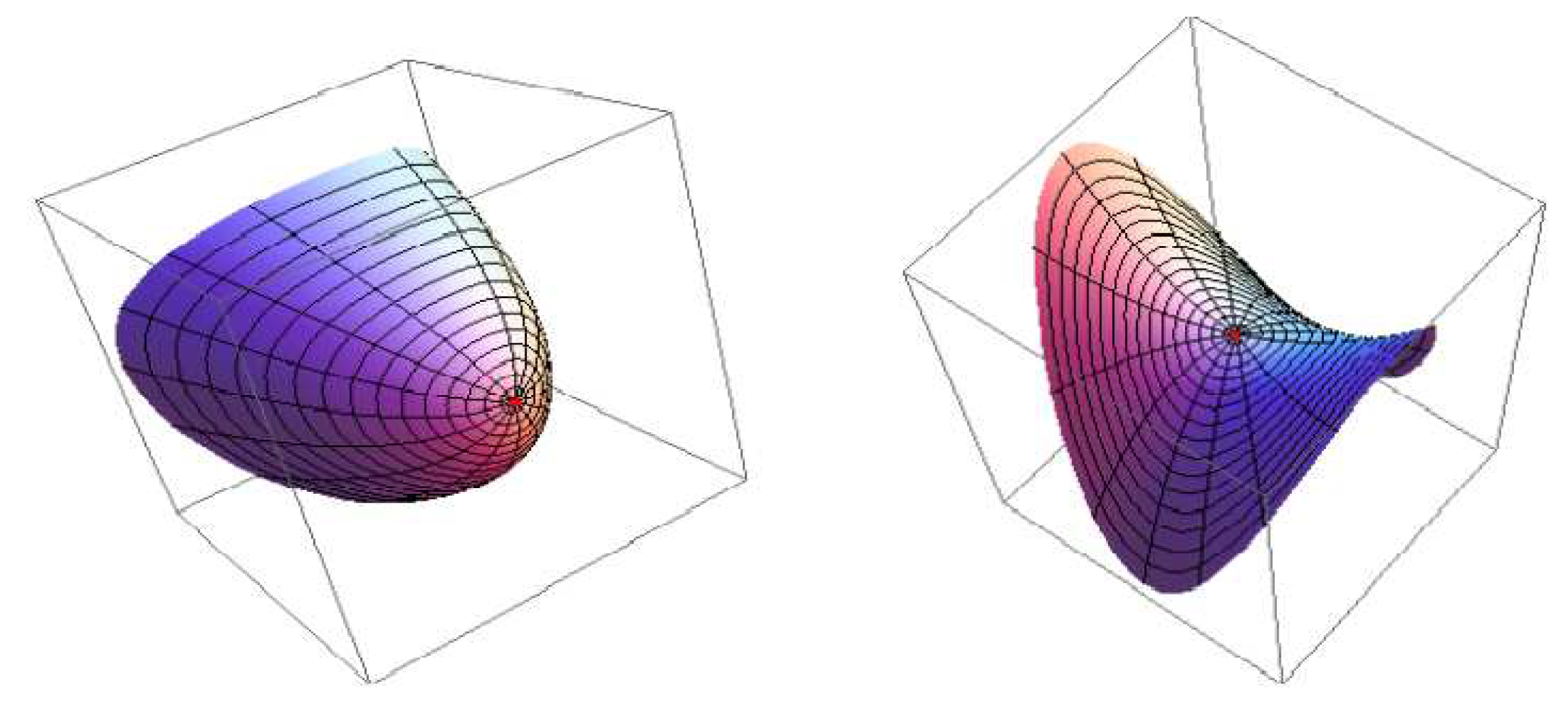
Figure 6. The elliptic paraboloids

z = x^{2} + 2 y^{2} (t o t h e l e f t) a n d z = x^{2} - 2 y^{2}

(to the right) (c.f., [21]).

Figure 6. The elliptic paraboloids

z = x^{2} + 2 y^{2} (t o t h e l e f t) a n d z = x^{2} - 2 y^{2}

(to the right) (c.f., [21]).

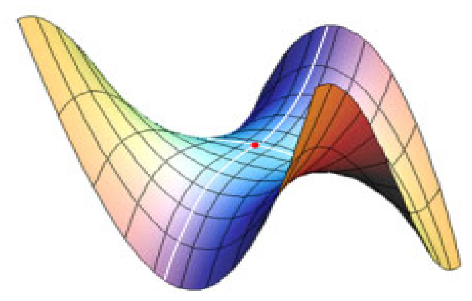
Figure 7. Planar points with quite different shapes(c.f., [21]).

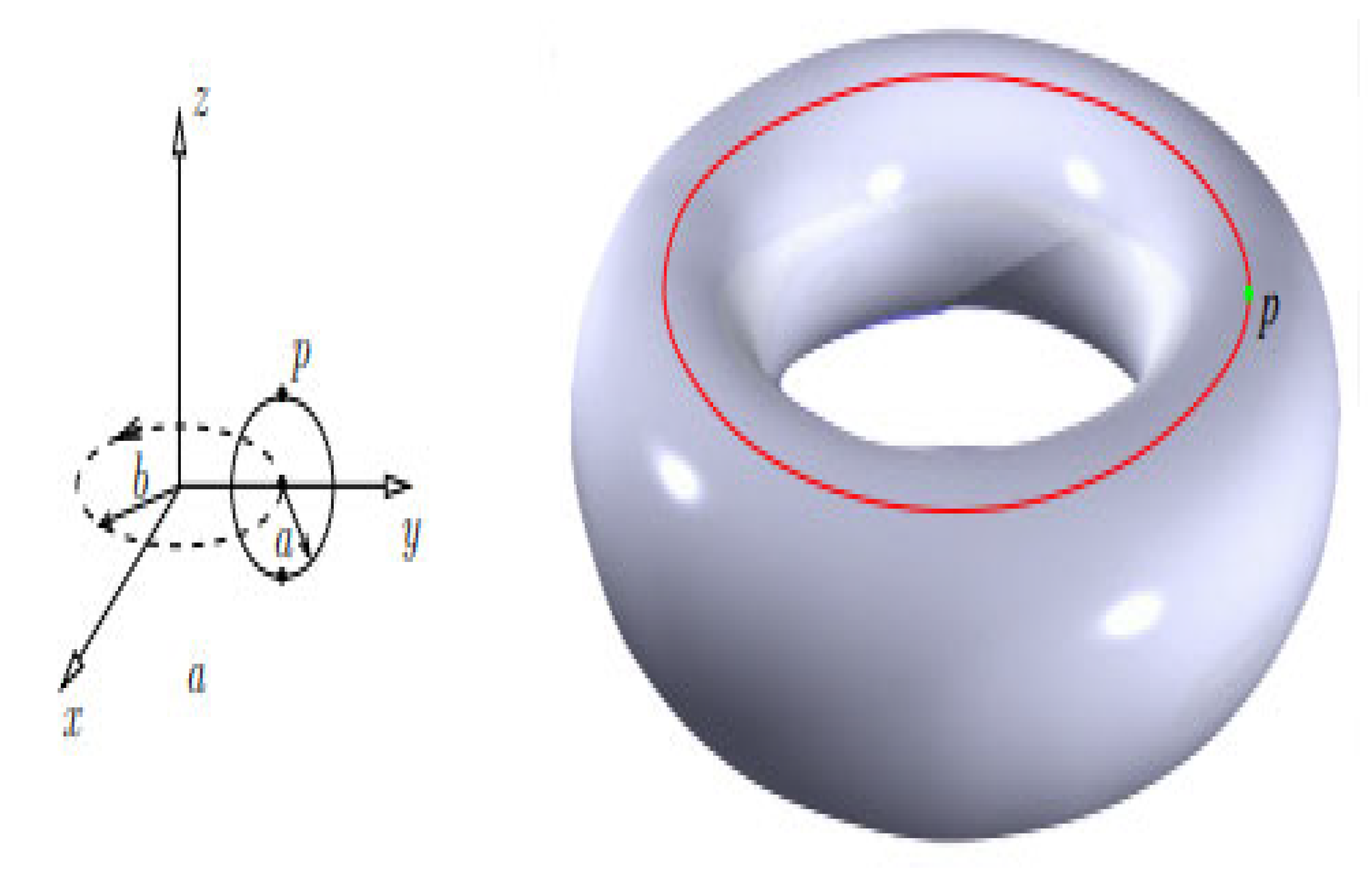
A torus as shown in Figure 8

2.3. Different Approach to Gaussian and Mean Curvatures (Angular Technique) (c.f., [22])

A new formulation (c.f., [22]) is introduced for Gaussian Curvature

K_{G}

and the Mean Curvature is

H

are defined as

K_{G} = K_{1} K_{2}

(2.25)

And

H = \frac{1}{2} (K_{1} + K_{2})

with K_{1}

and

K_{2}

as the principal curvatures are determined by:

K_{1} = \frac{B_{11}}{{(1 + {(\frac{\partial f}{\partial x_{1}^{’}})}^{2})}^{\frac{3}{2}}}, K_{2} = \frac{B_{22}}{{(1 + {(\frac{\partial f}{\partial x_{2}^{’}})}^{2})}^{\frac{3}{2}}}

(2.27)

where

x_{3} = f (x_{1}, x_{2})

defines the shape of the surface.

x_{1}^{’}

and

x_{2}^{’}

are parallel to the directions of the principal curvature, which are rotated through an angle

ω

with respect to

x_{1} and x_{2}

, and

\frac{\partial f}{\partial x_{1}^{’}} = c o s ω \frac{\partial f}{\partial x_{1}} - s i n ω \frac{\partial f}{\partial x_{2}}

(2.28)

\frac{\partial f}{\partial x_{2}^{’}} = s i n ω \frac{\partial f}{\partial x_{1}} + c o s ω \frac{\partial f}{\partial x_{2}}

(2.29)

B_{11} = \frac{\partial^{2} f}{\partial x_{1}^{2}} c o s^{2} ω - 2 \frac{\partial^{2} f}{\partial x_{1} \partial x_{2}} s i n ω c o s ω + \frac{\partial^{2} f}{\partial x_{2}^{2}} s i n^{2} ω = \frac{\partial^{2} f}{\partial x_{1}^{’ 2}}

(2.30)

B_{22} = \frac{\partial^{2} f}{\partial x_{1}^{2}} s i n^{2} ω + 2 \frac{\partial^{2} f}{\partial x_{1} \partial x_{2}} s i n ω c o s ω + \frac{\partial^{2} f}{\partial x_{2}^{2}} c o s^{2} ω = \frac{\partial^{2} f}{\partial x_{2}^{’ 2}}

(2.31)

The angle

ω

through which the coordinate frame is rotated to align the axes with the directions of the principal curvature at each point on the surface is given by

t a n 2 ω = \frac{- 2 (\frac{\partial^{2} f}{\partial x_{1} \partial x_{2}})}{(\frac{\partial^{2} f}{\partial x_{1}^{2}} - \frac{\partial^{2} f}{\partial x_{2}^{2}})}

(2.32)

A contour plot of Gaussian curvature indicates where structures occur on a surface. If both principal curvatures are non- zero, the surface is said to have double curvature [22].

Figure 10. (c.f., [22]).

K_{G}

are slab structures- related by the three regions (a), (b), and (c).

Figure 10. (c.f., [22]).

K_{G}

are slab structures- related by the three regions (a), (b), and (c).

2.4. Well Defined Functions and Bijective Functions

1. function f is said to be one-to-one, or injective, if and only if f(x) = f(y) implies x = y for all x, y in the domain of f. A function is said to be an injection if it is one-to-one. Alternative: A function is one-to-one if and only if f(x) ≠ f(y), whenever x ≠ y. This is the contrapositive of the definition.

2.A function f from A to B is called onto, or surjective, if and only if for every b ∈ B there is an element a ∈ A such that f(a) = b. Alternative: all co-domain elements are covered.

3. A function f is called a bijection if it is both one-to-one (injection) and onto (surjection).

Definition 2.14(c.f., [25])

The solution of the cubic equation

(2.33)

is characterized arbitrarily by

y = z - \frac{ε_{3}}{z}

(2.34)

w = y - \frac{b^{*}}{3 a^{*}}

(2.35)

z = \sqrt[3]{(- \frac{ε_{1}}{2}) \pm \sqrt{ε_{2}}},

(2.36)

ε_{1} = \frac{2 {(b^{*})}^{3}}{27} + \frac{d^{*}}{a^{*}} - \frac{b^{*} c^{*}}{3 {(a^{*})}^{2}},

(2.37)

ε_{2} = \frac{{(ε_{1})}^{2}}{4} + \frac{{(ε_{3})}^{3}}{27},

(2.38)

where

ε_{3}

is given by

ε_{3} = - \frac{2 {(b^{*})}^{2}}{3 {(a^{*})}^{2}} + \frac{c^{*}}{a^{*}}

(2.39)

ε_{2}

is called the discriminant of the cubic equation.

Preliminary Theorem(PT) 2.15 [26].

Let f be a function that is defined and differentiable on an open interval (c,d).

(1) If f^{'} (x) > 0 for all x \in (c, d), then f is increasing on (c, d)

(2.40)

If f^{'} (x) < 0 for all x \in (c, d), then f is decreasing on (c, d) .

(2.41)

2.5. Stability Analysis for Ordinary Differential Equations (ODEs) [27]

Equilibria are not always stable. Since stable and unstable equilibria play quite different roles in the dynamics of a system, it is useful to be able to classify equilibrium points based on their stability. Suppose that we have a set of autonomous ordinary differential equations, written in vector form:

\frac{d x}{d t} = f (x)

(2.42)

Suppose that

x^{*}

is an equilibrium point. By definition,

f (x^{*}) = 0.

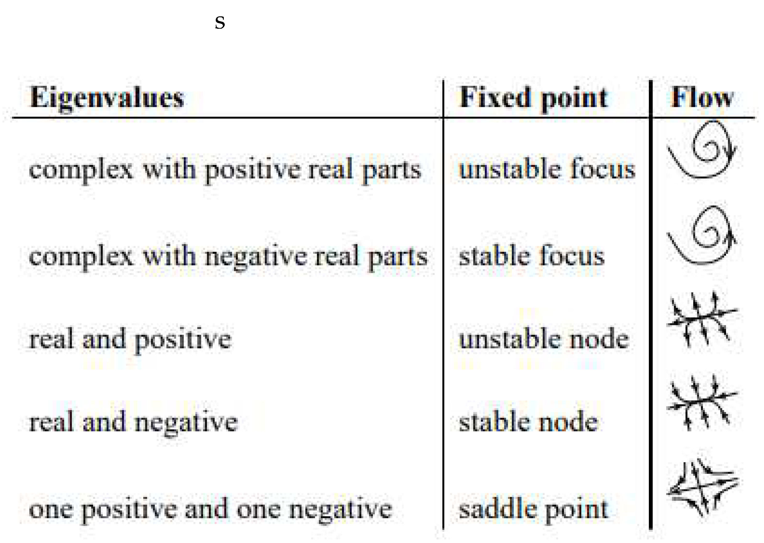
Theorem 2.16 (c.f., [27])An equilibrium point

x^{*}

of the differential equation 1 is stable if all the eigenvalues of

J^{*}

, the Jacobian evaluated at

x^{*}

, have negative real parts. The equilibrium point is unstable if at least one of the eigenvalues has a positive real part.

Figure 11. (c.f., [27]).

2.6. Scalar Curvature(Ricci Scalar), $R$ and Einestein Tensor, $℘$

The scalar curvature(Ricci Scalar),

R

(c.f., [15]) measures RCT’s contraction(c.f., (2.12))

R = R_{i j}^{(α)} g^{i j}, i, j = 1, 2, 3, \dots .

(2.43)

The two-dimensional Ricci Scalar,

R

[28] is twice as the Gaussian Curvature

K_{G}

(c.f., (2.25)),

R = 2 K_{G} = 2 K_{1} K_{2}

(2.44)

provided that

K_{1} and K_{2}

are determined by (2.27).

The Ricci scalar

R

[15] has a similar meaning to

K_{G}

R = l i m_{ϵ \to 0} \frac{6 n}{ϵ^{2}} [1 - \frac{A_{c u r v e d} (ϵ)}{A_{f l a t} (ϵ)}]

(2.45)

Ricci scalar completely captures the curvature of the surface.

The equations of motion of a classical theory like General Relativity can be derived directly from a suitable action by using the Euler-Lagrange equations, leading to the well-known Einstein equations [29]

G_{i j} = R_{i j}^{(α)} - \frac{R}{2} g_{i j} = \frac{8 π g ϖ_{i j}}{c^{4}}

(2.46)

where

G_{i j}

is the Curvature of Spacetime(Einstein tensor),

℘

R_{ij}^{(α)} defines spacetime - RCT

, namely

g_{i j}

R = R_{i j}^{(α)} g^{i j}, i, j = 1, 2, 3, \dots,

is the Ricci scalar or scalar curvature,

g

is the universal gravitational constant,

c

is the speed of light, and

ϖ_{i j}

are the components of the stress-energy tensor,

ϖ

,as a descriptor of spacetime- matter-energy distributions.

2.7. Maxima and Minima of Functions of Two Variables [30]

Suppose that

(a_{1}, b_{1})

is a critical point of

f (x, y)

(i.e,

\frac{\partial f (a_{1}, b_{1})}{\partial x} = 0 = \frac{\partial f (a_{1}, b_{1})}{\partial y}

). Let’s denote:

D = D (a_{1}, b_{1}) = f_{x x} (a_{1}, b_{1}) f_{y y} (a_{1}, b_{1}) - {[f_{x y} (a_{1}, b_{1})]}^{2}

(2.47)

This provides the critical point categories:

If $D > 0 and f_{x x} (a_{1}, b_{1}) > 0$ then there is a relative minimum at $(a_{1}, b_{1}) .$
If $D > 0 and f_{x x} (a_{1}, b_{1}) < 0$ then there is a relative maximum at $(a_{1}, b_{1}) .$
If $D < 0$ then the point $(a_{1}, b_{1}) is a saddle point .$
If $D = 0$ then the point $(a_{1}, b_{1})$ may be a relative minimum, relative maximum, or a saddle point. Other techniques would need to be used to classify the critical point.

2.8. Continuous Functions (c.f., [31])

Theorem 2.16

A function

f

is continuous at

x_{0}

if and only if

f

is defined on an open interval

(r, s)

containing

x_{0}

and for each

ε > 0

there is a

δ > 0

such that:

|f (x) - f (x_{0})| < ε

(2.48)

whenever

|x - x_{0}| < δ

2.9. The Maclauren’s Series of $l n (1 - x)$ for $x a r o u n d z e r o$ (Shaw,2015)

l n (1 - x) = - \sum_{n = 1}^{\infty} \frac{x^{n}}{n}

(2.49)

3. The Fim and Its Inverse for the Stable M/G/1 QM

According to [32], the maximum entropy (ME) state probability of the generalized geometric solution of a stable M/G/1 queue (c.f., Figure. 12), subject to normalisation, mean queue length (MQL), L and server utilisation,

ρ

(<1) is given by

Figure 12.

p (n) = \{\begin{matrix} 1 - ρ, n = 0 \\ (1 - ρ) g x^{n}, n \geq 1 \end{matrix}

(3.1)

where

g = \frac{ρ^{2}}{(L - ρ) (1 - ρ)}, x = \frac{L - ρ}{L}

and

L = \frac{ρ}{2} (1 + \frac{1 + ρ C_{s}^{2}}{1 - ρ})

ρ

= 1 –

p (0) and β = C_{s}^{2} .

p (n)

of (3.1) reads as:

p (n) = \{\begin{matrix} 1 - ρ, n = 0 \\ \frac{2 ρ {(\frac{1 + ρ β}{1 - ρ} - 1)}^{n - 1}}{({(\frac{1 + ρ β}{1 - ρ} + 1)}^{n}}, n > 0, w i t h β = C_{s}^{2} \end{matrix}

(3.2)

Theorem 3.1 The underlying QM satisfies:

(i) FIM reads as

[g_{i j}] = (\begin{matrix} \frac{1}{{(1 - ρ)}^{2}} & 0 \\ 0 & \frac{- 1}{{(β + 1)}^{2}} \end{matrix})

(3.3)

(ii) {(d s)}^{2} = (\frac{1}{{(1 - ρ)}^{2}}) {(d ρ)}^{2} - \frac{1}{{(β + 1)}^{2}} {(d β)}^{2}

(3.4)

(iii) [

g^{i j}

] reads as

[g^{i j}] = \frac{a d j [g_{i j}]}{Δ} = (\begin{matrix} {(1 - ρ)}^{2} & 0 \\ 0 & - {(β + 1)}^{2} \end{matrix})

(3.5)

Proof

(i)

Case I:

p (0) = 1 - ρ

. Thus,

L (x; θ) = l n (p (x; θ)) = l n (1 - ρ),

θ = θ_{1} = ρ

(3.6)

Ψ (θ) = - l n (1 - ρ)

(3.7)

Therefore,

\partial_{1} = \frac{\partial Ψ}{\partial ρ} = \frac{1}{1 - ρ} (3.8) . \partial_{1} \partial_{1} = \frac{\partial^{2} Ψ}{\partial ρ^{2}} = \frac{1}{{(1 - ρ)}^{2}}

(3.9)

FIM is given by:

[g_{i j}] = [\frac{\partial^{2} Ψ}{\partial ρ^{2}}] = [\frac{1}{{(1 - ρ)}^{2}}]

(3.10)

[g^{i j}]

reads as

[g^{i j}] = {[g_{i j}]}^{- 1} = [{(1 - ρ)}^{2}]

(3.11)

Case II: For

n > 0, p (n) = \frac{2 ρ {(\frac{1 + ρ β}{1 - ρ} - 1)}^{n - 1}}{({(\frac{1 + ρ β}{1 - ρ} + 1)}^{n}}

. Therefore, the coordinate system is two-dimensional satisfying:

L (x; θ) = l n (p (x; θ)) = l n (1 - ρ) + l n 2 - l n (β + 1) + n l n (\frac{ρ (1 + β)}{2 + ρ (β - 1)})

(3.12)

where

θ = (θ_{1}, θ_{2}) = (ρ, β), w i t h β = C_{s}^{2}

(3.13)

We have

Ψ (θ) = l n (β + 1) - l n (1 - ρ) - l n 2

(3.14)

Thus, we have

\partial_{1} = \frac{1}{1 - ρ} \partial_{2} = \frac{1}{β + 1}, \partial_{11} = \frac{1}{{(1 - ρ)}^{2}}, \partial_{1} \partial_{2} = \partial_{2} \partial_{1} = 0, \partial_{22} = - \frac{1}{{(β + 1)}^{2}}

(3.15)

FIM is given by

[g_{i j}]

(\begin{matrix} \frac{1}{{(1 - ρ)}^{2}} & 0 \\ 0 & \frac{- 1}{{(β + 1)}^{2}} \end{matrix})

(3.16). This completes the proof of (i)

It could be verified that

{(d s)}^{2} = (\frac{1}{{(1 - ρ)}^{2}}) {(d ρ)}^{2} - \frac{1}{{(β + 1)}^{2}} {(d β)}^{2}

(c.f., (3.4))

Finally, after some manipulation, it could be shown that:

[g^{i j}] = \frac{a d j [g_{i j}]}{Δ} = (\begin{matrix} {(1 - ρ)}^{2} & 0 \\ 0 & - {(β + 1)}^{2} \end{matrix})

(c.f., (3.5))

4. The α(. OR $\nabla^{(α)}$ )-Connection of the M/G/1 QM

(2.8) implies:

Γ_{11, 1}^{(α)} = (\frac{1 - α}{{(1 - ρ)}^{3}}), Γ_{11, 1}^{(α)} = \frac{(1 - α)}{{(1 - ρ)}^{3}}

(4.1)

Γ_{11}^{1 (α)} = \frac{1 - α}{(1 - ρ)}, Γ_{11}^{1 (0)} = \frac{1}{(1 - ρ)}

(4.2)

Γ_{22}^{2 (α)} = - \frac{1 - α}{(1 + β)}, Γ_{22}^{2 (0)} = - \frac{1}{(1 + β)}

(4.3)

Engaging the same logic, RCT’s remaining components can be determined.

5. Variational Inference, KD,JD,RÉNYI AND s AB DIVERGENCES OF STABLE M/G/1 QM

5.1. KD and JD Divergences of Stable M/G/1 QM

The following theorem characterizes both KD and JD of (2.5) and (2.6) respectively.

Theorem 5.1 The underlying QM satisfies:

(i) K (p, q) = E_{θ_{p}} [l n (\frac{p (x; θ_{p})}{q (x; θ_{q})})] = l n ((\frac{1 - ρ_{p}}{1 - ρ_{q}}) (\frac{1 + β_{q}}{1 + β_{p}}) {[(\frac{ρ_{q} (2 + ρ_{q} {(β}_{q} - 1)}{ρ_{p} (2 + ρ_{p} {(β}_{p} - 1)}) (\frac{1 + β_{q}}{1 + β_{p}})]}^{L_{p}})

(5.1)

L_{p}

defines the Mean Queue Length at

p .

Also,

(ii) J D (p, q) = = l n {[(\frac{ρ_{q} (2 + ρ_{q} {(β}_{q} - 1)}{ρ_{p} (2 + ρ_{p} {(β}_{p} - 1)}) (\frac{1 + β_{q}}{1 + β_{p}})]}^{{(L}_{p} - L_{q})}

(5.2)

where

L_{p}

L_{q}

defines the Mean Queue Length at

p a n d q r e s p e c t i v e l y .

Proof

To show (i), the case for

n = 0

is straightforward. For

n > 0,

It could be verified that, using (3.2), we have

After some few mathematical steps, it could be seen that:

l n (\frac{p (n)}{q (n)}) = l n (\frac{ρ_{p}}{ρ_{q}}) + l n (\frac{1 - ρ_{p}}{1 - ρ_{q}}) + (n - 1) l n (\frac{ρ_{p} (1 + β_{p})}{ρ_{q} (1 + β_{q})}) + n l n (\frac{(2 + ρ_{q} {(β}_{q} - 1)}{(2 + ρ_{p} {(β}_{p} - 1)})

(5.3)

By (5.4), it follows that KD will be determined by

K (p, q) = l n [(\frac{1 - ρ_{p}}{1 - ρ_{q}}) (\frac{1 + β_{q}}{1 + β_{p}})] + L_{p} (l n ((\frac{ρ_{q} (2 + ρ_{q} {(β}_{q} - 1)}{ρ_{p} (2 + ρ_{p} {(β}_{p} - 1)}) (\frac{1 + β_{p}}{1 + β_{q}})))

(5.4)

(

n = 0, 1,2, \dots ., a n d L_{p} = \sum_{n = 0}^{\infty} n p (n)

)

= l n (\frac{1 - ρ_{p}}{1 - ρ_{q}}) (\frac{1 + β_{q}}{1 + β_{p}}) {[(\frac{ρ_{q} (2 + ρ_{q} {(β}_{q} - 1)}{ρ_{p} (2 + ρ_{p} {(β}_{p} - 1)}) (\frac{1 + β_{q}}{1 + β_{p}})]}^{L_{p}}

(c.f., (5.1))

This completes the proof of (i).

To prove (ii), we have by (2.6) and (5.5

)

Following some mathematical steps, (5.2) could be easily verified.

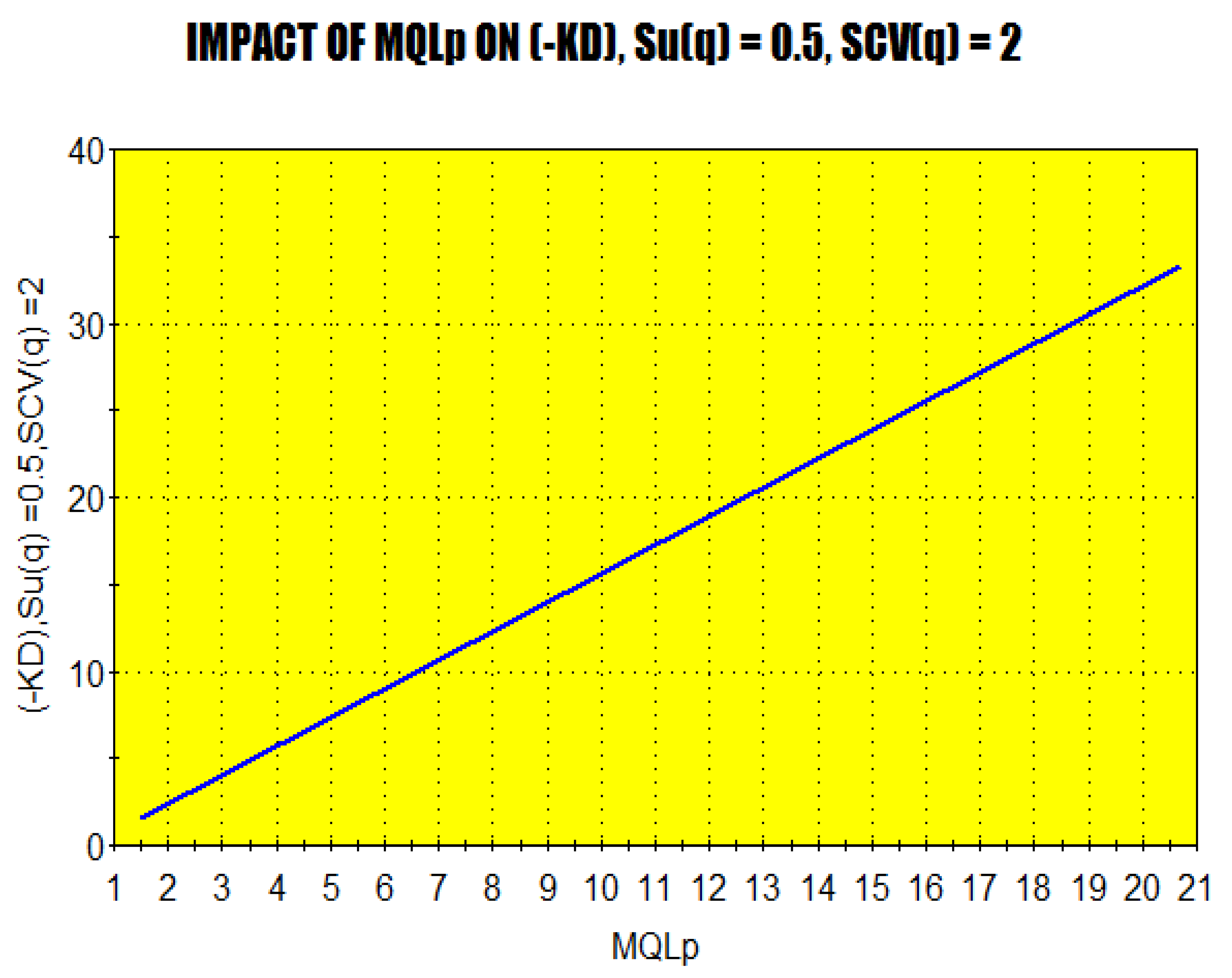
Clearly it follows from (5.2), that JD is also zero if and only if

p = q .

This present a novel result which declares the compressibility of the underlying QM if and only if it is stable or when p and q are identical, (i.e.,

ρ_{p} = ρ_{q}, β_{p} = β_{q})

It is observed by (5.1), that JD is dependent on

ρ_{q}, β_{q}

and the MQL of Pollaczeck-Khinchin Formula of a stable M/G/1 QM at

p, L_{p}

(which is dependent on

ρ_{p} a n d β_{p})

. To examine the impact of

L_{p}

on JD, the following experiment is introduced.

Figure 13.

Figure 13 depicts that KD is a negative decreasing function in MQL at p,

L_{p} .

This justifies that the increase of

L_{p}

will have a significant impact on the decrease of KD. In other words, the increase of MQL at p, would enforce the distance between p and q to increase in magnitude.

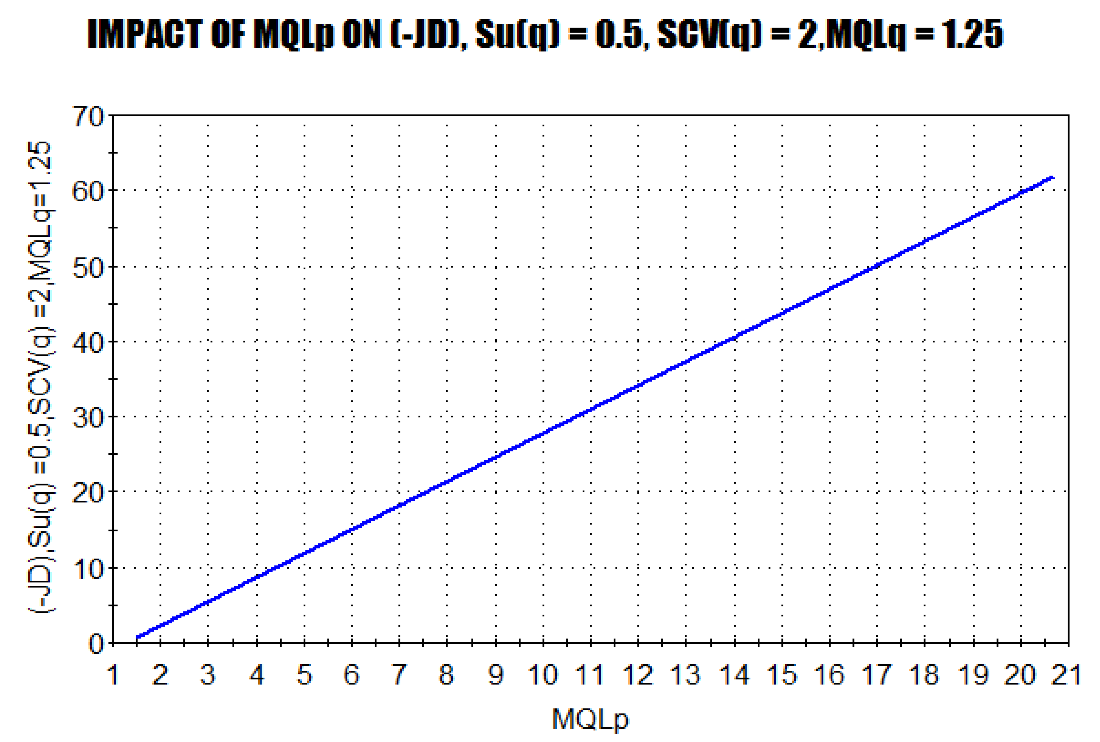
Compressibility of M/G/1 QM could be identified visually by presenting the following numerical experiment:

Figure 14.

The findings of figure 14, show that the increase of MQL at p impacts the the stable M/G/1 QM’s solenoidability of. As it observed that M/G/1 QM is solenoidal at the steady state phase of the QM. By the increase of

L_{p} s u c h t h a t L_{p} \neq L_{q}

, the stable M/G/1 QM is no longer solenoidal. This shows the direct impact of queueing parameters on the visualization of the regions of solenoidability of the stable M/G/1 QM.

Meanwhile, we have

Figure 15.

As observed by Figure 15, KD decreases and vanishes at

ρ_{p}

= 0.5. by the increase of

ρ_{p}

, KD decreases and tends to

- \infty

when the underlying M/G/1 QM approaches instability (

ρ_{p}

= 1).

Figure 16. (c.f., [27]).

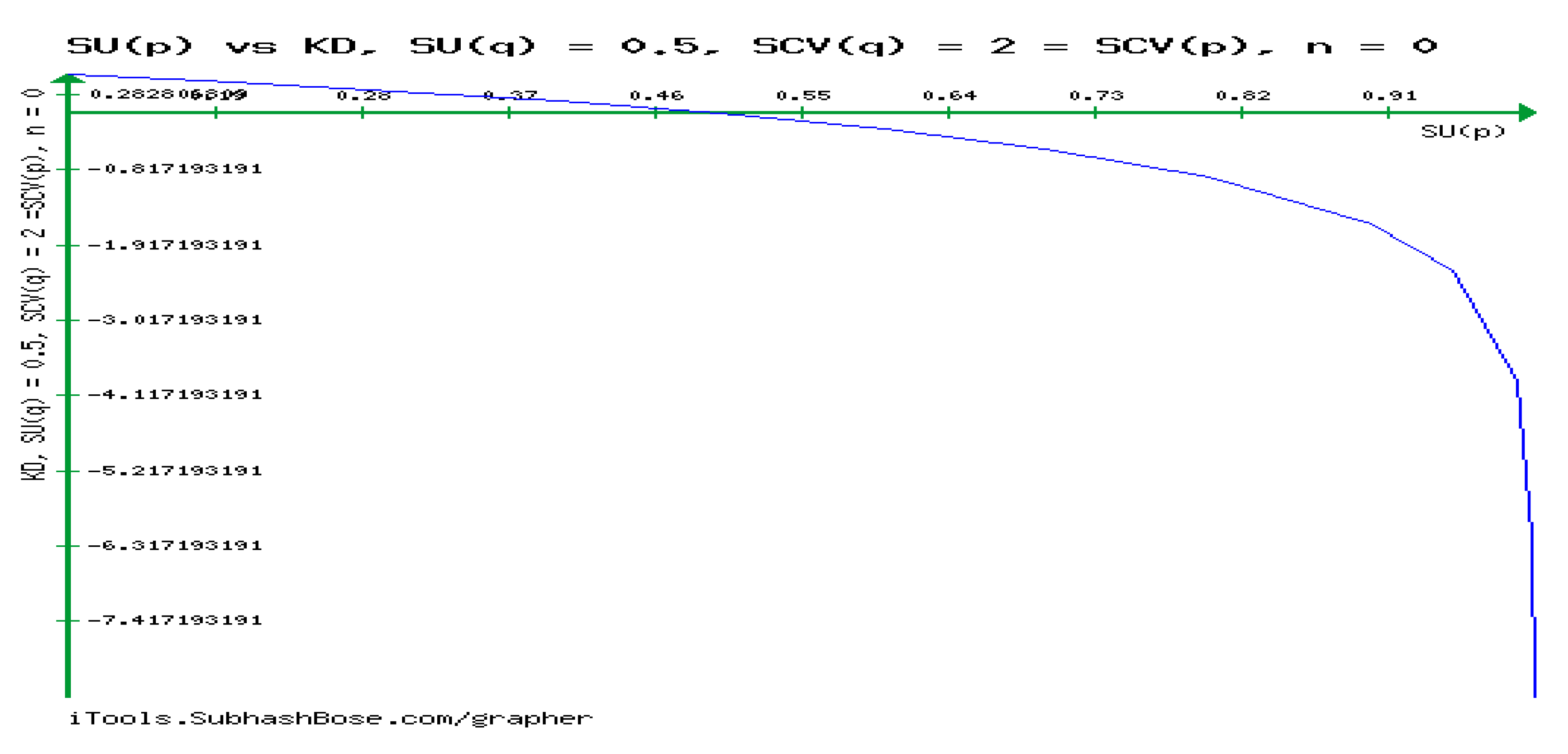
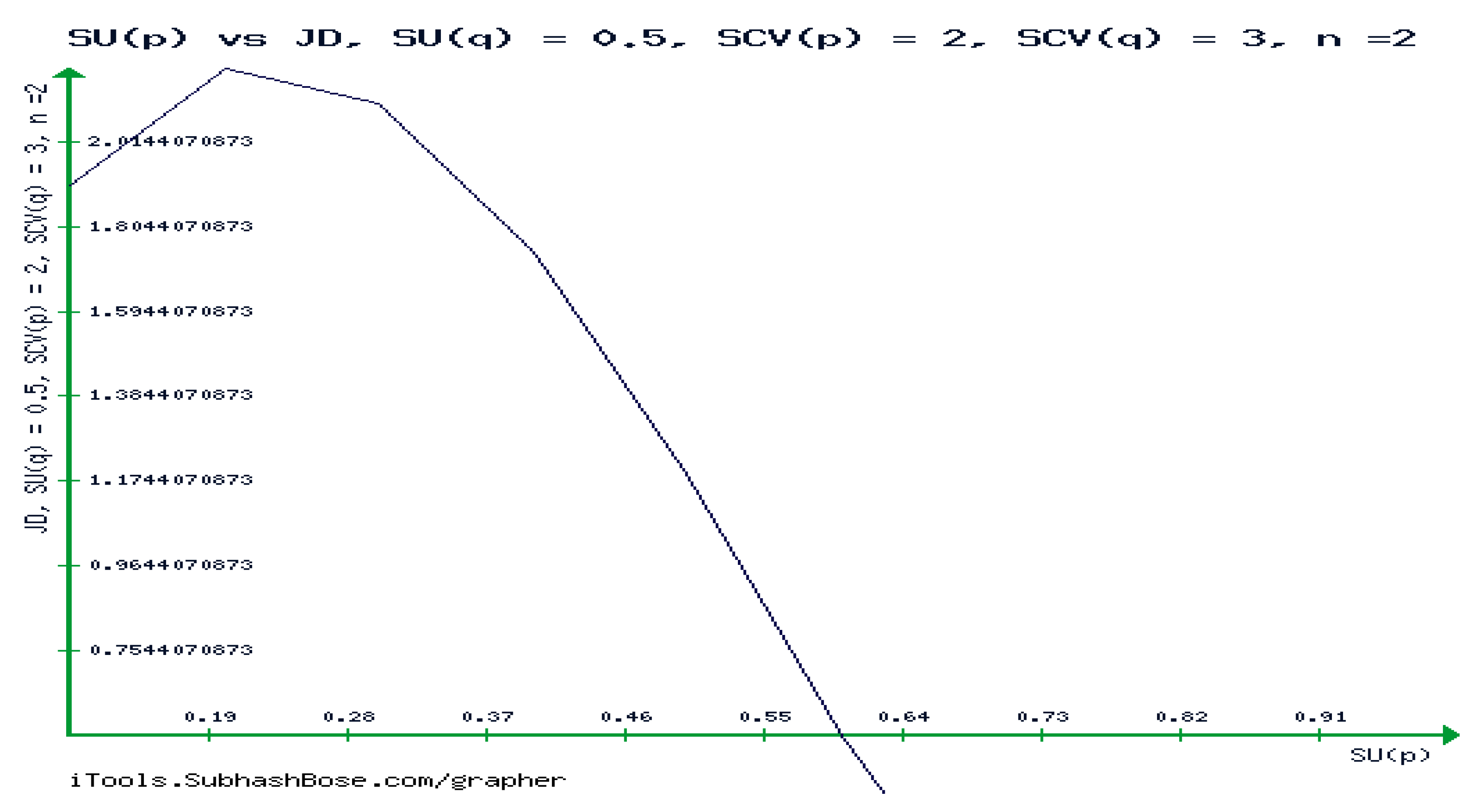
As observed by Figure 16, for n =2, KD increases for permissible values of SU(p) and starts to decrease at SU(p) = as we go along. Then, it decreases when SU(p) = 0.4. Afterwards, KD decreases unsoundly , speeding rapidly to

- \infty

. In this physical interpretation, stability has a significant impact on the behaviour of KD. In principle, it is uncovered that the stability of the M/G/1 QM has a significant impact on the performance of KD.

5.2. Rényi Divergence of Stable M/G/1 QM

Theorem 5.2 The underlying queueing system satisfies:

R D (p, q) = D_{R}^{γ} (p | |q) = \{\begin{matrix} \frac{1}{(γ - 1)} (γ \ln (1 - ρ_{p}) + (1 - γ) l n (1 - ρ_{q})), n = 0 \\ \ln {[(\frac{ρ_{p} (1 + β_{q}) (1 - ρ_{p})}{(1 - ρ_{q}) (1 + β_{p})})]}^{ρ_{p}} {+ \frac{1}{(γ - 1)} \ln [\sum_{n = 1}^{\infty} p (n) (\frac{ρ_{p} (1 + β_{p}) (2 + ρ_{q} {(β}_{q} - 1))}{ρ_{q} (2 + ρ_{p} {(β}_{p} - 1)) (1 + β_{q})})]}^{n (γ - 1)}, n > 0 \end{matrix}

(5.5)

Proof

R D (p, q) = D_{R}^{γ} (p | |q) = \frac{1}{(γ - 1)} l n ({({(p (0))}^{γ} (q (0))}^{1 - γ}) = \frac{1}{(γ - 1)} l n ({({(1 - ρ_{p})}^{γ} (1 - ρ_{q})}^{1 - γ})

(5.6)

It could be easily checked that

D_{R}^{γ} (p | |q)

of (5.6) that:

D_{R}^{γ} (p | |q) = \frac{1}{(γ - 1)} (γ \ln (1 - ρ_{p}) + (1 - γ) l n (1 - ρ_{q}))

as required.

It could be verified that for

n > 0,

R D (p, q) = l n {(\frac{(1 - ρ_{p}) (1 + β_{q})}{(1 - ρ_{q}) (1 + β_{p})})}^{ρ_{p}} + \frac{1}{(γ - 1)} l n (\sum_{n = 1}^{\infty} {(\frac{ρ_{p} (1 + β_{p}) (2 + ρ_{q} {(β}_{q} - 1)}{ρ_{q} (2 + ρ_{p} {(β}_{p} - 1) (1 + β_{q})})}^{n (γ - 1)} p (n))

(c.f., (5.5))

We are done.

γ \to 1,

\underset{γ \to 1}{l i m} D_{R}^{γ} (p | |q) = \lim_{γ \to 1} \frac{1}{(\sum_{n = 0}^{\infty} {(p (n))}^{γ} {(q (n))}^{1 - γ})} (\sum_{n = 0}^{\infty} {[γ (p (n))}^{γ - 1} {(q (n))}^{1 - γ} + {(1 - γ) (q (n))}^{- γ} {(p (n))}^{γ})

= \lim_{γ \to 1} \frac{1}{(\sum_{n = 0}^{\infty} {(p (n))}^{γ} {(q (n))}^{1 - γ})} \sum_{n = 0}^{\infty} (1)

\infty

Data R

É

NYI DIVERGENCE,RD

CASE ONE

Figure 17.

It is shown by Figure 17,RD is drastically decreasing until SU(p) is greater than 1, RD becomes imaginary number, i.e., the instability of M/G/1 QM occurs , RD becomes imaginary!!!

It is observed that for

n = 0, γ \to 1 (s h a n n o n i a n p h a s e), D_{R,}^{1} (p | |q) = l n (\frac{1 - ρ_{p}}{1 - ρ_{q}})

CASE TWO

Figure 18.

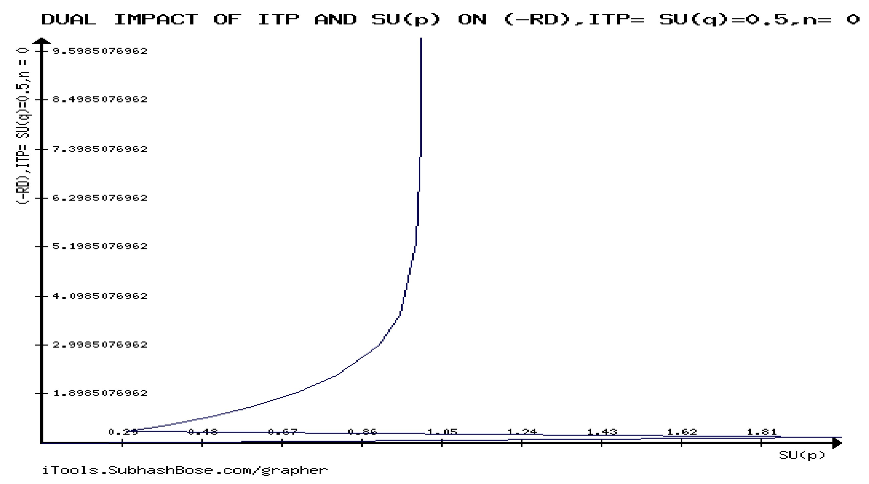
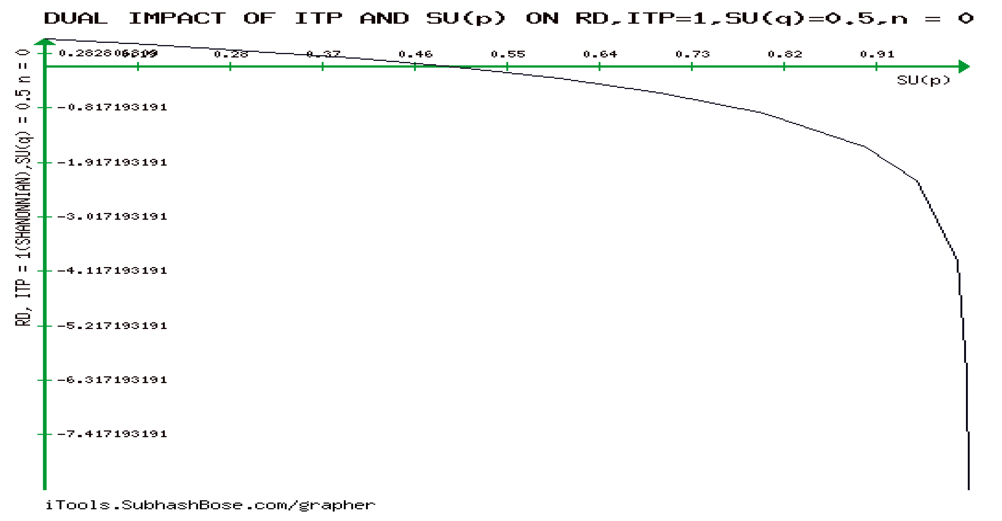
Following Figure 18, The decreasability of RD is clear because of the dual impact of Su(p) and ITP on RD.

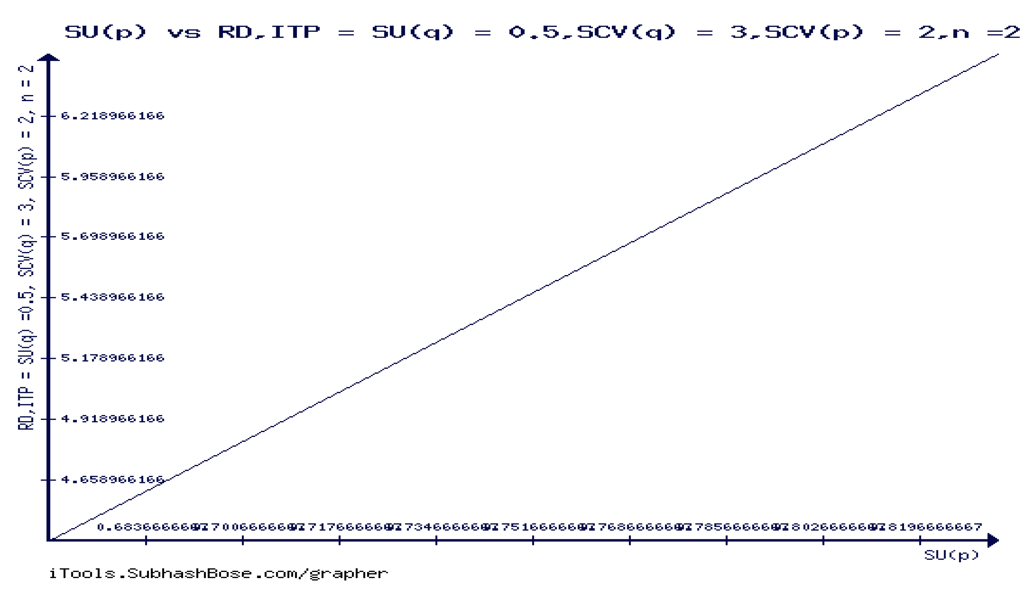
CASE TWO, RD,

n = 2

Figure 19.

As observed from figure 19, that RD increases rapidly by the increase of

ρ_{p}

. It is expected that RD approaches infinity as

ρ_{p}

approaches unity(i.e, M/G/1 QM is unstable at

p)

. To show this, we can take the limit of (5.9) as

ρ_{p}

approaches unity. This directly implies that:

D_{R}^{0.5}

(p||

ρ_{q} = 0.5, β_{q} = 3) \to \ln 0 + 3 l n (3) - 2 l n (p (1) (1 - p (1))

, or

The devised corresponding absolute limiting value of RD is

{| D}_{R}^{0.5}

(p||

ρ_{q} = 0.5, β_{q} = 3) | \to | \ln 0 + 3 l n (3) - 2 l n (p (1) (1 - p (1)) |

\infty

5.3. sAB divergence, $D_{s, A B}^{η, γ}$ (p||q) of Stable M/G/1 QM

Before going into details, we need to prove the following important lemma as it is needed in the proofs.

Lemma 5.3

p (n)

of (3.2) rewrites to

p (n) = \{\begin{matrix} 1 - ρ, n = 0 \\ \frac{2 ρ (1 - ρ)}{(1 + β)} {(\frac{ρ^{2} (1 + β)}{(1 - ρ) L})}^{n}, n > 0, w i t h β = C_{s}^{2} \end{matrix}

(5.10)

where

L = \frac{ρ}{2} (1 + \frac{1 + ρ C_{s}^{2}}{1 - ρ})

ρ

= 1 –

p (0)

and

{β = C}_{s}^{2}

.

Proof For

n = 0

, it is immediate by (3.2)

As for

n > 0

By the MQL formula, we have

L = \frac{ρ}{2} (1 + \frac{1 + ρ β}{1 - ρ})

. Hence,

(2 + ρ (β - 1)) = \frac{2 (1 - ρ) L}{ρ}

. This implies :

\frac{2 ρ {(\frac{1 + ρ β}{1 - ρ} - 1)}^{n - 1}}{({(\frac{1 + ρ β}{1 - ρ} + 1)}^{n}} = \frac{2 ρ {(\frac{ρ (1 + β)}{1 - ρ})}^{n - 1}}{({(\frac{(2 + ρ (β - 1))}{1 - ρ})}^{n}} = \frac{2 ρ {(\frac{ρ (1 + β)}{1 - ρ})}^{n - 1}}{({(\frac{\frac{2 (1 - ρ) L}{ρ}}{1 - ρ})}^{n}} = \frac{2 ρ (1 - ρ)}{(1 + β)} {(\frac{ρ^{2} (1 + β)}{(1 - ρ) L})}^{n}

(5.11)

By (5.11) and (3.2), the proof follows.

Theorem 5.4

{s A B}_{n = 0}

divergence vanishes,

D_{s, A B}^{η, γ}

(5.12)

(p||q) = 0

Proof For

n = 0, p (n) = 1 - ρ_{p}, q (n) = 1 - ρ_{q}

. hence, it follows by (2.10) that :

D_{s, A B}^{γ, η} (p | |q) = 0

(c.f,(5.12))

Theorem 5.5 For

n \neq 0,

sAB divergence is determined by

D_{s, A B}^{η, γ} (p | | q) = l n [{(\sum_{n = 1}^{\infty} {(\frac{ρ_{p}^{2} (1 + β_{p})}{(1 - ρ_{p}) L_{p}})}^{n (γ + η)})}^{\frac{1}{η (η + γ)}} {(\sum_{n = 1}^{\infty} {(\frac{ρ_{q}^{2} (1 + β_{q})}{(1 - ρ_{q}) L_{q}})}^{n (γ + η)})}^{\frac{1}{γ (η + γ)}} {(\sum_{n = 1}^{\infty} {(\frac{ρ_{p}^{2} (1 + β_{p})}{(1 - ρ_{p}) L_{p}})}^{n γ} {(\frac{ρ_{q}^{2} (1 + β_{q})}{(1 - ρ_{q}) L_{q}})}^{n η})}^{- \frac{1}{γ η}}]

(5.13)

for

(γ, η) ϵ R^{2}

such that

γ \neq 0, η \neq 0 a n d γ + η \neq 0

Proof We have

p (n) = \frac{2 ρ_{p} (1 - ρ_{p})}{(1 + β_{p})} {(\frac{ρ_{p}^{2} (1 + β_{p})}{(1 - ρ_{p}) L_{p}})}^{n}

q (n) = \frac{2 ρ_{q} (1 - ρ_{q})}{(1 + β_{q})} {(\frac{ρ_{q}^{2} (1 + β_{q})}{(1 - ρ_{q}) L_{q}})}^{n}

(c.f. (5.11) of Lemma 5.3)

Following (2.10),

D_{s, A B}^{γ, η} (p | |q) = [\frac{1}{η (η + γ)} l n (\sum_{n = 1}^{\infty} {(\frac{2 ρ_{p} (1 - ρ_{p})}{(1 + β_{p})} {(\frac{ρ_{p}^{2} (1 + β_{p})}{(1 - ρ_{p}) L_{p}})}^{n})}^{γ + η}) + \frac{1}{γ (η + γ)} l n (\sum_{n = 1}^{\infty} {(\frac{2 ρ_{q} (1 - ρ_{q})}{(1 + β_{q})} {(\frac{ρ_{q}^{2} (1 + β_{q})}{(1 - ρ_{q}) L_{q}})}^{n})}^{γ + η}) - \frac{1}{γ η} l n (\sum_{n = 1}^{\infty} {(\frac{2 ρ_{p} (1 - ρ_{p})}{(1 + β_{p})} {(\frac{ρ_{p}^{2} (1 + β_{p})}{(1 - ρ_{p}) L_{p}})}^{n})}^{γ} {(\frac{2 ρ_{q} (1 - ρ_{q})}{(1 + β_{q})} {(\frac{ρ_{q}^{2} (1 + β_{q})}{(1 - ρ_{q}) L_{q}})}^{n})}^{η})]

(5.14)

It could be checked that RHS of (5.14) reduces after some lengthy computation to

D_{s, A B}^{γ, η} (p | |q) = l n [{(\sum_{n = 1}^{\infty} {(\frac{ρ_{p}^{2} (1 + β_{p})}{(1 - ρ_{p}) L_{p}})}^{n (γ + η)})}^{\frac{1}{η (η + γ)}} {(\sum_{n = 1}^{\infty} {(\frac{ρ_{q}^{2} (1 + β_{q})}{(1 - ρ_{q}) L_{q}})}^{n (γ + η)})}^{\frac{1}{γ (η + γ)}} {(\sum_{n = 1}^{\infty} {(\frac{ρ_{p}^{2} (1 + β_{p})}{(1 - ρ_{p}) L_{p}})}^{n γ} {(\frac{ρ_{q}^{2} (1 + β_{q})}{(1 - ρ_{q}) L_{q}})}^{n η})}^{- \frac{1}{γ η}}]

(c.f.,(5.13))

Numerical experiment for

D_{s, A B}^{γ, η} (p | |q)

Data one:

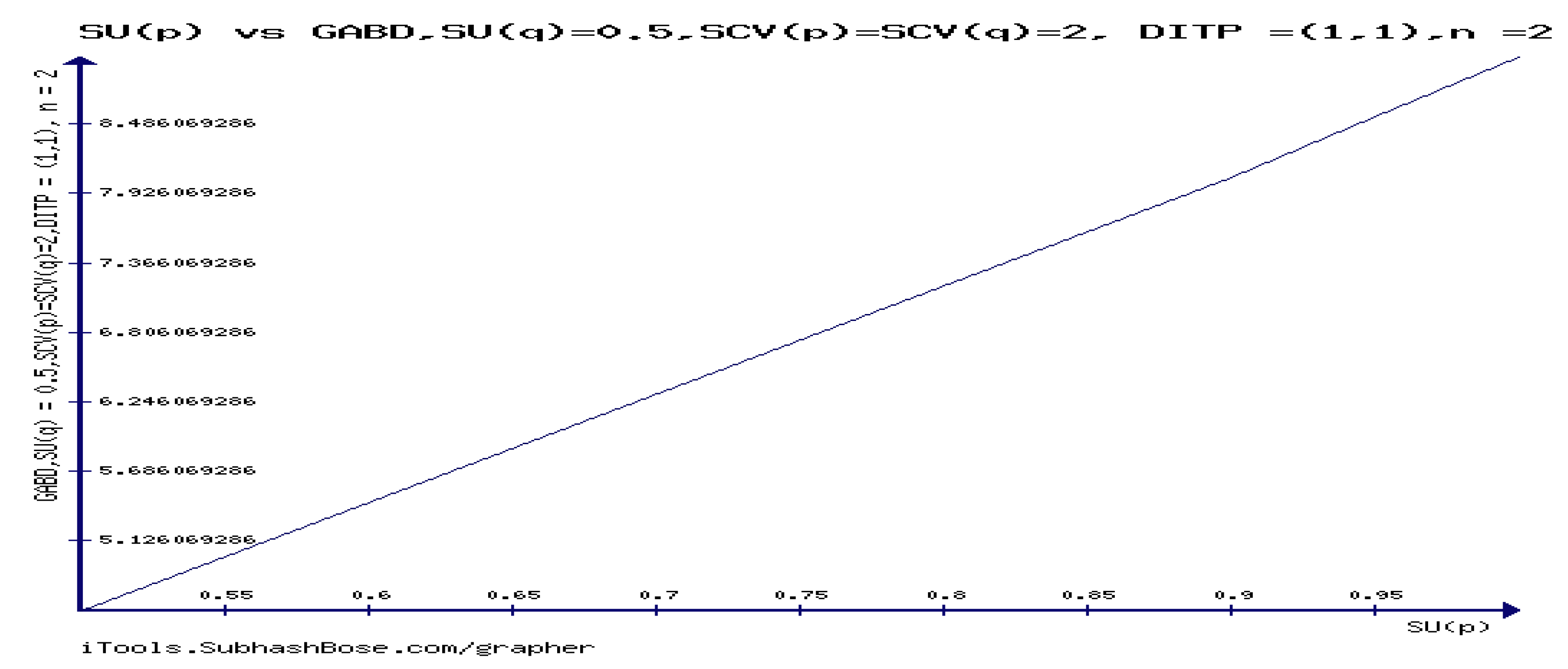
Following (5.13), it can be verified after some manipulation, that for

ρ_{q} = 0.5, β_{p} = β_{q} = 2, n = 2

DITP = (

γ, η

)=(1,1),

D_{s, A B}^{1,1} (p | |q)

l n [\frac{\sqrt (\frac{{(\frac{6 ρ_{p}}{2 + ρ_{p}})}^{2} + {(\frac{6 ρ_{p}}{2 + ρ_{p}})}^{4}}{{(\frac{12}{5})}^{2} + {(\frac{12}{5})}^{4}})}{(\frac{72 ρ_{p}}{5 (2 + ρ_{p})}) + {(\frac{72 ρ_{p}}{5 (2 + ρ_{p})})}^{2}}

Figure 20.

The increasability of the GENERALIZED ALPHA BETA DIVERGENCE(GABD) as SU(p) increases is obvious from figure 20.

DATA TWO

After some lengthy computation, it could be verified that for the non-extensive information theoretic dual, DITP=

(γ, η) = (0.5,0.5)

n = 2

({D_{s, A B}^{(0.5,0.5)} (p| |q))}_{(ρ_{q = 0.5}, β_{q = 3, β_{p} = 2)}}

l n (\frac{3 (\sum_{n = 1}^{2} {(\frac{6 ρ_{p}}{2 + ρ_{p}})}^{n})}{2 ρ_{p} (1 - ρ_{p}) {(\sum_{n = 1}^{2} {(\frac{6 ρ_{p}}{2 + ρ_{p}})}^{\frac{n}{2}})}^{4}})

ρ_{p} \to 1 (i n s t a b i l t y p h a s e

of M/G/1 QM ,

D_{A B}^{(0.5,0.5)} (p | | q_{ρ_{q = 0.5}, β_{q = 0.5}}) \to \infty

6. Investigations of the Developability of the Stable M/G/1 QM ,RICCI CURVATURE (RCT) tENSOR and QT-IG Unifiers

6.1. Investigation of Developability of M/G/1 QM and Finding Its Ricci Curvature Tensor (RCT)

Theorem 6.1 The stable M/G/1 QM

i) Has a zero 0-Gaussian curvature, for which the stable M/G/1 QM would be developable.

ii) Has a non-zero Ricci Tensor

iii) Is non-developable minimal surface under Monge Technique, with a zero Mean Curvature

iv) Is developable under Angular Technique if and only if M/G/1 QM unstable

v) If the underlying QM is unstable, then the Mean Curvature is negative under Angular Technique. The converse statement is not always true.

vi) The first principal curvature,

K_{1}

under the Angular Technique satisfies the inequality

K_{1} < 1

(6.1)

vii) The second principal curvature,

K_{2} i s β - d e p e n d e n t a n d i s n e g a t i v e

under the Angular Technique.

viiii) Under the Angular Technique, the second principal curvature,

K_{2}

tends to zero as

β \to \infty .

Proof

For i), we must prove :

K^{(α)} = \frac{R_{1212}^{(α)}}{d e t (g_{i j})} = 0

(6.2)

It could be verified that,

R_{1212}^{(α)} = 0

(6.3)

d e t (g_{i j}) = - \frac{1}{{(β + 1)}^{2} {(1 - ρ)}^{2}} \neq 0

. Hence,

K^{(α)} = \frac{R_{1212}^{(α)}}{d e t (g_{i j})} = 0

, which proves that the underlying QM is developable subject to

α - G a u s s i a n c u r v a t u r e

ii) We must prove that:

R_{i k}^{(α)} = R_{i j k l}^{(α)} g^{j l} is non-zero

We have

R_{1212}^{(α)} g^{11} + R_{1112}^{(α)} g^{12} + R_{1211}^{(α)} g^{21} + R_{1212}^{(α)} g^{22}

Engaging the same procedure as in (6.2), we have

R_{11}^{(α)} = R_{12}^{(α)} = R_{22}^{(α)} = 0 (6.3) . R_{21}^{(α)} = - \frac{1 - α}{{(1 - ρ)}^{2}}, R_{21}^{(0)} = - \frac{1}{{(1 - ρ)}^{2}}

(6.5)

H e n c e, R_{21}^{(α)} \neq 0

(6.6). The corresponding Ricci Curvature Tensor is given by

(R C T) = (\begin{matrix} 0 & - \frac{1}{{(1 - ρ)}^{2}} \\ 0 & 0 \end{matrix})

ρ \to 1, R_{21}^{(0)} \to - \infty .

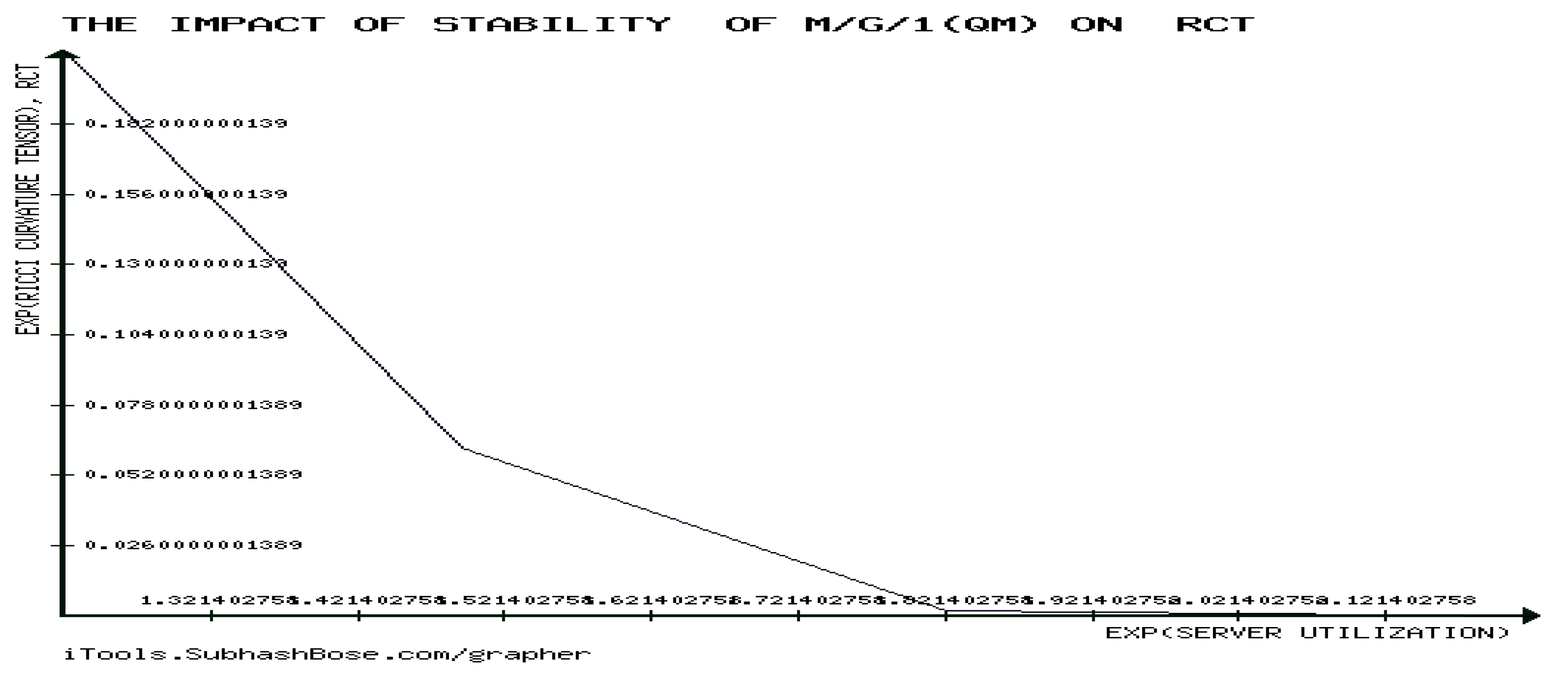
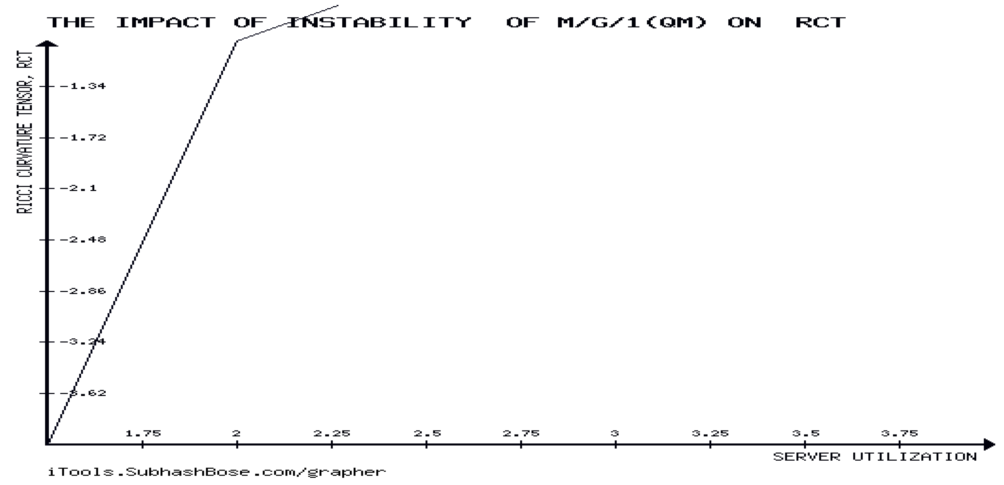
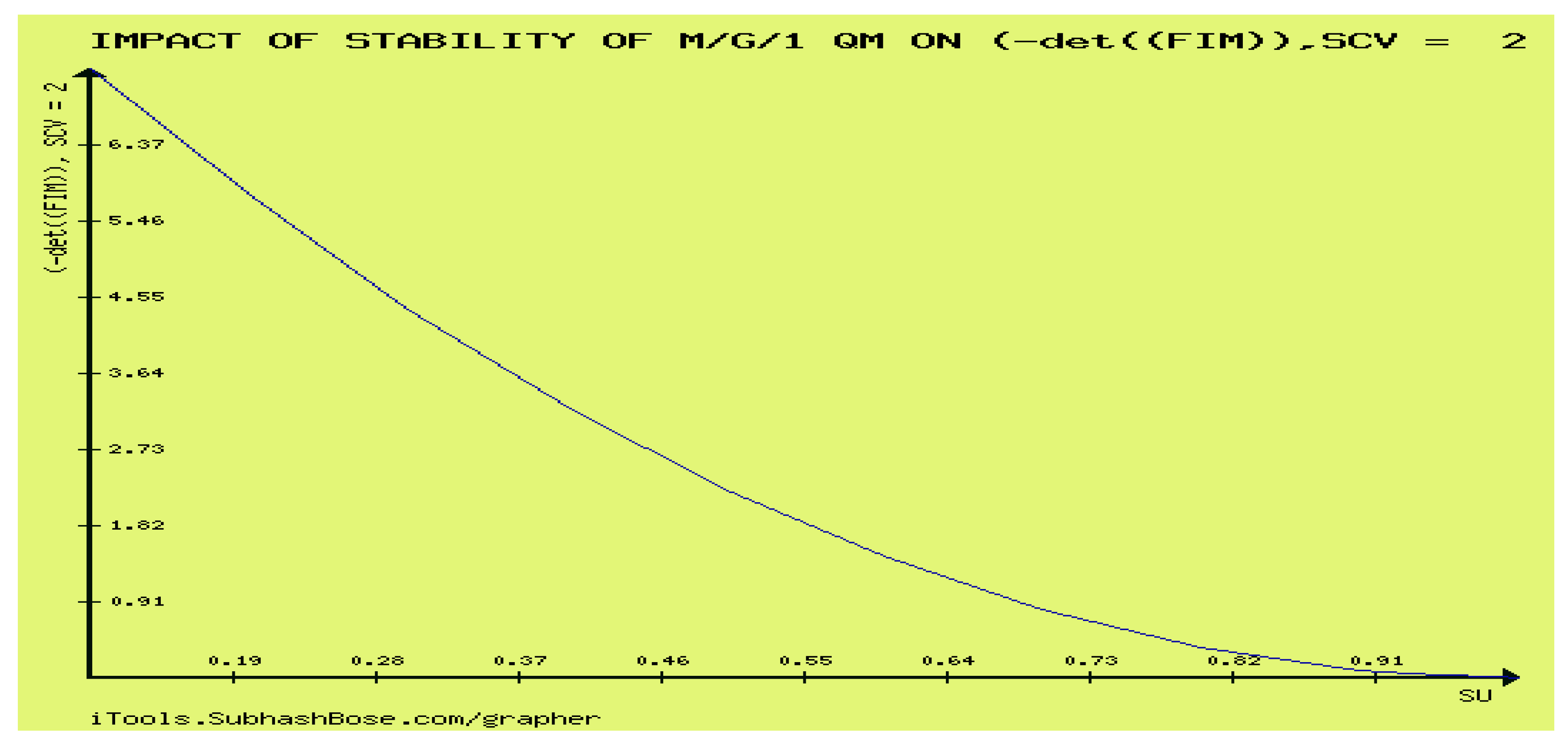
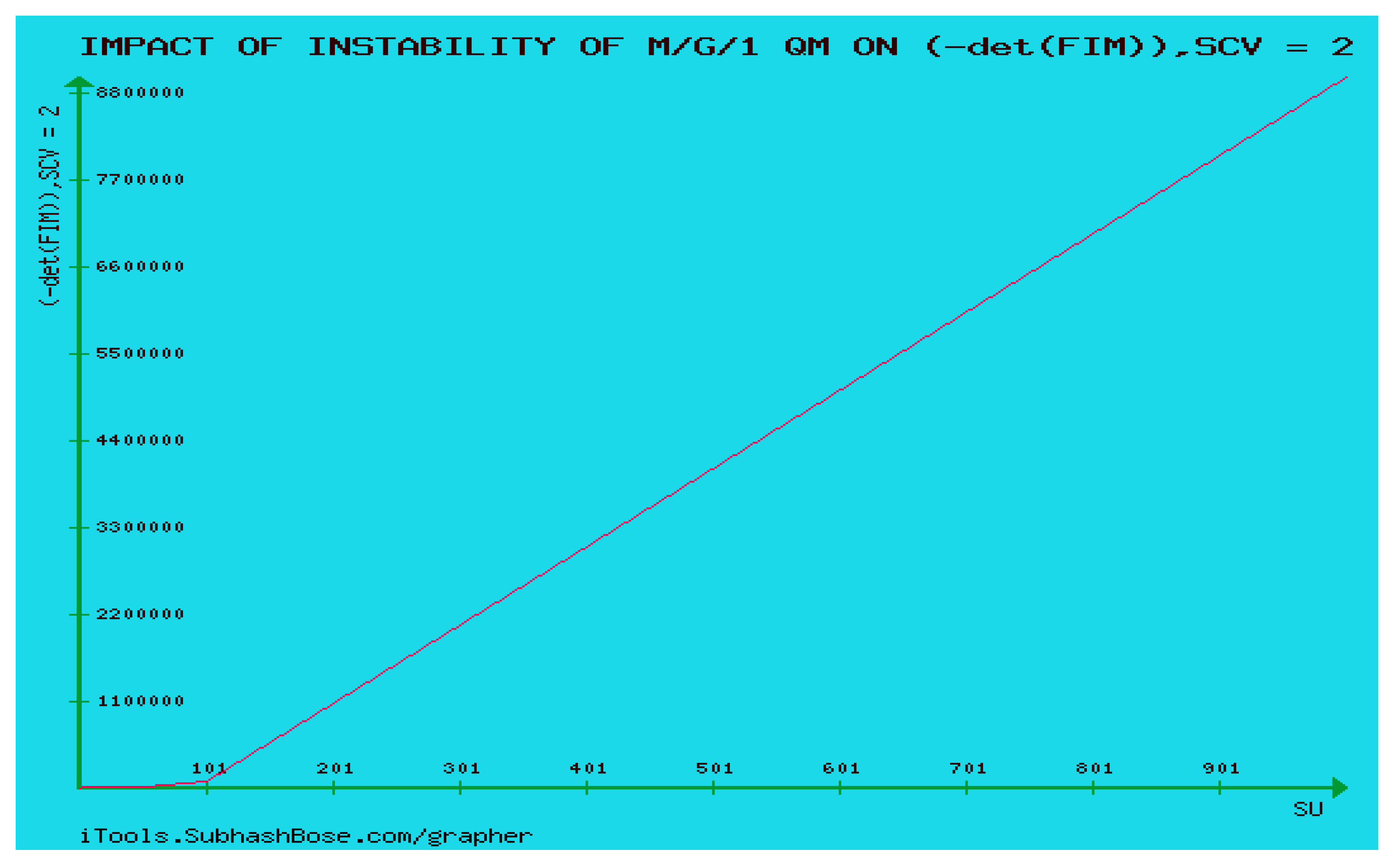
The highlights the significant influence of instability in a specific type of the underlying QM, by providing supporting evidence on how RCT is significantly impacted by the stability analysis of the system. The also shows that

ρ

, represented by

R_{21}^{(0)}

,affects the behavior of RCT, and Figure 21 demonstrates that the stability phase of the M/G/1 QM causes RCT to decrease as ρ increases.

Figure 21.

whereas in Figure 22, RCT increasability in

ρ

is caused by the underlying QM’s instability.

Figure 22.

iii) Following (3.14) and (3.15), it is clear that

Thus, we have

\partial_{1} = \frac{1}{1 - ρ} \partial_{2} = \frac{1}{β + 1}, \partial_{11} = \frac{1}{{(1 - ρ)}^{2}}, \partial_{1} \partial_{2} = \partial_{2} \partial_{1} = 0, \partial_{22} = - \frac{1}{{(β + 1)}^{2}}

(3.15)

The Gaussian Curvature

K_{G} = \frac{L N - M^{2}}{E G - F^{2}}

(c.f.,(2.23))

E = {(\partial_{1})}^{2} = {(\frac{1}{1 - ρ})}^{2}, F = \partial_{1} \partial_{2} = 0, G = {(\partial_{2})}^{2} = \frac{1}{{(β + 1)}^{2}},

L = \partial_{11} = \frac{1}{{(1 - ρ)}^{2}}, M = \partial_{12} = 0, N = \partial_{22} = - \frac{1}{{(β + 1)}^{2}}

And the Mean Curvature is

H = \frac{1}{2} (\frac{L G - 2 M F + N E}{E G - F^{2}})

(c.f., (2.24))

Therefore, it is obtained that

K_{G} = \frac{L N - M^{2}}{E G - F^{2}} = - \frac{\frac{1}{{(1 - ρ)}^{2}} \frac{1}{{(β + 1)}^{2}}}{\frac{1}{{(1 - ρ)}^{2}} \frac{1}{{(β + 1)}^{2}}} = - 1, ρ \neq 1 (t h e u n d e r l y i n g Q M i s s t a b l e), β \neq - 1

(6.7)

(β = C_{s}^{2} i s n e v e r n e g a t i v e b y d e f a u l t)

Since

K_{G}

- 1,

it follows by the non- developability of the underlying QM and its minimal surface under Monge Technique.

The Mean Curvature is

H = \frac{1}{2} (\frac{L G - 2 M F + N E}{E G - F^{2}}) = \frac{\frac{1}{2} (\frac{1}{{(1 - ρ)}^{2}} \frac{1}{{(β + 1)}^{2}} - \frac{1}{{(1 - ρ)}^{2}} \frac{1}{{(β + 1)}^{2}})}{\frac{1}{{(1 - ρ)}^{2}} \frac{1}{{(β + 1)}^{2}}} = 0

(6.8)

Hence, iii) is done.

iv) Following the Angular Technique, it can be verified that the calculations of the principal curvatures

K_{1} a n d K_{2}

are determined by

K_{1} = \frac{(1 - ρ)}{{(1 + {((1 - ρ))}^{2})}^{\frac{3}{2}}}, K_{2} = \frac{- (1 + β)}{{(1 + {((1 + β)}^{2})}^{\frac{3}{2}}}

(6.9)

K_{G} = K_{1} K_{2} = \frac{- (1 - ρ)}{{(1 + {((1 - ρ))}^{2})}^{\frac{3}{2}}} \frac{(1 + β)}{{(1 + {((1 + β)}^{2})}^{\frac{3}{2}}}

(6.10)

and

H = \frac{1}{2} (K_{1} + K_{2}) = \frac{1}{2} (\frac{(1 - ρ)}{{(1 + {((1 - ρ))}^{2})}^{\frac{3}{2}}} - \frac{(1 + β)}{{(1 + {((1 + β)}^{2})}^{\frac{3}{2}}})

(6.11)

The axial rotator angle

Ꙍ

reads as

t a n 2 Ꙍ = \frac{- 2 (\partial_{1} \partial_{2})}{(\partial_{11} - \partial_{22})} = 0

(6.12)

This implies,

Ꙍ = 0, 2 π, 4 π, \dots .

It appears from (6.10), that

K_{G} = 0 (e q u i v a l e n t l y, t h e u n d e r l y i n g Q M i s d e v e l o p a b l e)

if and only if

\frac{(1 - ρ)}{{(1 + {((1 - ρ))}^{2})}^{\frac{3}{2}}} \frac{(1 + β)}{{(1 + {((1 + β)}^{2})}^{\frac{3}{2}}} = 0

(6.13)

This implies that:

either (1 - ρ) = 0 (equivalently, ρ = 1) or (1 + β) = 0

(6.14)

The second possibility (

(1 + β) = 0)

generates a contradiction as

β

is never negative.

Moreover,

{l i m}_{β \to \infty} K_{G} = - \frac{(1 - ρ)}{{(1 + {((1 - ρ))}^{2})}^{\frac{3}{2}}} {l i m}_{β \to \infty} \frac{(1 + β)}{{(1 + {((1 + β)}^{2})}^{\frac{3}{2}}} = 0

(6.15)

Linking the findings of (6.13) and (6.15) completes the proof of iv).

As for v), it has been obtained that

H = \frac{1}{2} (K_{1} + K_{2}) = \frac{1}{2} (\frac{(1 - ρ)}{{(1 + {((1 - ρ))}^{2})}^{\frac{3}{2}}} - \frac{(1 + β)}{{(1 + {((1 + β)}^{2})}^{\frac{3}{2}}})

(6.11)

This directly implies

H < \frac{1}{2} \frac{(1 - ρ)}{{(1 + {((1 - ρ))}^{2})}^{\frac{3}{2}}}

(6.16)

It is clear that

1 + {((1 - ρ))}^{2} > 0

holds for all the possible values of

ρ .

Consequently, if

(1 - ρ) = 0

ρ = 1

(equivalently, the underlying QM is unstable), itid="FD99 follows that

H < 0

To prove the necessity condition, assume that

H < 0

. This generates two possibilities:

The first possibility,

\frac{1}{2} \frac{(1 - ρ)}{{(1 + {((1 - ρ))}^{2})}^{\frac{3}{2}}} < 0

. This implies

ρ > 1

. Hence, M/G/1 QM is unstable.

The second possibility,

\frac{1}{2} \frac{(1 - ρ)}{{(1 + {((1 - ρ))}^{2})}^{\frac{3}{2}}} > 0

. This implies

ρ < 1

. Hence, M/G/1 QM is stable.

This justifies that the converse statement is not always true. The proof of v) is complete.

To show vi), we have

K_{1} = \frac{(1 - ρ)}{{(1 + {((1 - ρ))}^{2})}^{\frac{3}{2}}}

(c.f., (6.9))

Since the underlying M/G/1 QM is assumed to be stable. Hence,

ρ \in (0,1) .

Thus, we have

1 > {(1 - ρ)}^{2} > 0 o r 2 > {(1 - ρ)}^{2} + 1 > 1 .

Therefore,

2^{\frac{3}{2}} > {(1 + {((1 - ρ))}^{2})}^{\frac{3}{2}} > 1

. Consequently,

\frac{1}{2^{\frac{3}{2}}} < \frac{1}{{(1 + {((1 - ρ))}^{2})}^{\frac{3}{2}}} < 1 . This implies \frac{(1 - ρ)}{2^{\frac{3}{2}}} < \frac{(1 - ρ)}{{(1 + {((1 - ρ))}^{2})}^{\frac{3}{2}}} < (1 - ρ) < 1

(6.17)

By (6.17), it holds that

K_{1} < 1 .

vii) we have by (6.9),

K_{2} = \frac{- (1 + β)}{{(1 + {((1 + β)}^{2})}^{\frac{3}{2}}}, w h i c h i s o f c o u r s e a β - d e p e n d e n t f u n c t i o n

The stability of M/G/1 QMenforces the condition

β > 1

to hold. The negativity of

K_{2}

is clear.

viii) Immediate from (6.15).

6.2. Revealing Novel QT-IG Unifiers and Discovering Their Algebraic Structures

Throughout this section, the following novel unifiers between both queueueing theoretic and information geometric structures of the stable M/G/ 1 QM are established by the following two unifiers,

φ_{1} (ρ) = K_{1} = \frac{(1 - ρ)}{{(1 + {((1 - ρ))}^{2})}^{\frac{3}{2}}}

(6.19)

φ_{2} (β) = K_{2} = \frac{- (1 + β)}{{(1 + {((1 + β))}^{2})}^{\frac{3}{2}}}

(6.19)

Theorem 6.2. For the above devised unifiers (c.f., (6.18) and (6.19)), it holds that

φ_{1}

is a well-defined function

ii) φ_{1} = \{\begin{matrix} l i e s i n t h e i n t e r v a l (0,1), ρ \in (0,1) \\ 0, ρ = 1 \\ < 0, ρ > 1 \end{matrix}

(6.20)

i i i) φ_{1}

is one-to –one.

iv)

φ_{1}

is onto

φ_{1}

is bijection, with animaginary inverse

φ_{1}^{- 1}

determined by

φ_{1}^{- 1} (ρ) = 1 \mp {((z - 1) + \frac{(3 + \frac{1}{ρ^{2}})}{z})}^{\frac{1}{2}}

(6.21)

where

z = \sqrt[3]{- \frac{1}{2 ρ^{2}} \pm i \sqrt{\frac{1}{{12 ρ}^{4}} + 1 + \frac{1}{2 ρ^{2}} + \frac{1}{27 ρ^{6}}}}, i = \sqrt{- 1}

vi)

φ_{2}

is a well-defined function

vii) φ_{2} = \{\begin{matrix} < - \frac{2}{5^{\frac{3}{2}}}, β \in (0,1) \\ - \frac{2}{5^{\frac{3}{2}}}, β = 1 \\ > - \frac{2}{5^{\frac{3}{2}}}, β > 1 \end{matrix}

(6.22)

v i i i) φ_{2}

isone-to –one

φ_{2}

is onto

xi)

φ_{2}

is bijection, with an imaginary inverse

φ_{2}^{- 1}

(i.e., a complex number)determined by

φ_{2}^{- 1} (β) = - 1 \mp {((z - 1) + \frac{(3 + \frac{1}{β^{2}})}{z})}^{\frac{1}{2}}

(6.23)

where

z = \sqrt[3]{- \frac{1}{2 β^{2}} \pm i \sqrt{\frac{1}{{12 β}^{4}} + 1 + \frac{1}{2 β^{2}} + \frac{1}{27 β^{6}}}}, i = \sqrt{- 1}

xii) The underlying QM has inverse of

ρ u n i f i e r, n a m e l y, φ_{1}^{- 1}

satisfies

|1 - φ_{1}^{- 1} (ρ)| < 5 + \frac{{(1 + (\frac{101}{54})}^{\frac{1}{6}}}{ρ^{2}}

(6.24)

xiii) The underlying of inverse of

β u n i f i e r, n a m e l y, φ_{2}^{- 1}

satisfies

|1 - φ_{2}^{- 1} (β)| < (1 + {(\frac{101}{54})}^{\frac{1}{6}} + \frac{1}{{(\frac{101}{54})}^{\frac{1}{6}}} + \frac{3 β^{2}}{{(\frac{101}{54})}^{\frac{1}{6}}})

(6.25)

xiv)

T h e i n c r e a s a b i l t y a n d d e c r e a s a b i l i t y o f φ_{1}

ρ

are undecidable.

xv)

φ_{2} i s f o r e v e r i n c r e a s i n g i n β

and is never decreasing in

β

To prove i), it is enough to show that for all

ρ_{1}, ρ_{2} \in (0,1)

such that

φ_{1} (ρ_{1}) = φ_{1} (ρ_{2})

, then

ρ_{1} a n d ρ_{2}

should never be distinct.

Let

φ_{1} (ρ_{1}) = φ_{1} (ρ_{2})

. After some lengthy mathematical steps, (6.26)id="FD99 reduces to

{(ρ}_{1} - ρ_{2}) {(ρ}_{1} + ρ_{2} - 2) [({(1 - ρ_{1})}^{2} {(1 - ρ_{2})}^{2} ({(1 - ρ_{1})}^{2} + {(1 - ρ_{2})}^{2} - 2))] = 0

(6.28)

Equation (6.28) generates three possible cases:

Case 1 : ρ_{1} - ρ_{2} = 0 . H e n c e ρ_{1} = ρ_{2} (contradiction to ρ_{1} \neq ρ_{2})

(6.29)

Case 2 : ρ_{1} + ρ_{2} - 2 = 0 . H e n c e ρ_{1} + ρ_{2} = 2 (contradiction, \sin ce M / G / 1 is a stable QM, ρ_{1}, ρ_{2} \in (0,1))

(6.30)

Case 3 : [({(1 - ρ_{1})}^{2} {(1 - ρ_{2})}^{2} ({(1 - ρ_{1})}^{2} + {(1 - ρ_{2})}^{2} - 2))] = 0

(6.31)

ρ_{1}, ρ_{2} \in (0,1),

following mathematical analysis it holds that

Therefore,

[({(1 - ρ_{1})}^{2} {(1 - ρ_{2})}^{2} ({(1 - ρ_{1})}^{2} + {(1 - ρ_{2})}^{2} - 2))] < 0,

which contradicts (6.29).

Based on the above analysis and by (6.29), i) follows.

ii) we have by (6.18),

φ_{1} (ρ) = K_{1} = \frac{(1 - ρ)}{{(1 + {((1 - ρ))}^{2})}^{\frac{3}{2}}} .

Since

ρ \in (0,1)

, it could be verified that

2 > 1 + {((1 - ρ))}^{2} > 0 . Hence, \frac{1}{{(1 + {((1 - ρ))}^{2})}^{\frac{3}{2}}} \in (0, \frac{1}{2}) . Therefore, 0 < φ_{1} (ρ) = \frac{(1 - ρ)}{{(1 + {((1 - ρ))}^{2})}^{\frac{3}{2}}} < \frac{1}{2} < 1

(6.33)

The case

φ_{1} (1) = 0

is clear. Also, for

ρ > 1,

it is immediate that

φ_{1} (ρ) < 0

. This completes the proof of ii).

iii) It suffices to show that for all

ρ_{1}, ρ_{2} \in (0,1)

such that

φ_{1} (ρ_{1}) = φ_{1} (ρ_{2})

, then

ρ_{1} = ρ_{2}

holds. The proof is clearly immediate from (6.29).

iv) From the definition,

φ_{1} (ρ) = \frac{(1 - ρ)}{{(1 + {((1 - ρ))}^{2})}^{\frac{3}{2}}}

. Every

\frac{(1 - ρ)}{{(1 + {((1 - ρ))}^{2})}^{\frac{3}{2}}}

is characterized by

ρ .

This clearly proves the surjectivity of

φ_{1} .

Hence, iv) follows.

v) Clearly,

φ_{1}

is a bijection. To calculate the inverse of

φ_{1}, n a m e l y φ_{1}^{- 1}

. Define

φ_{1} (ρ) = y

. Hence,

\frac{{(1 + {((1 - ρ))}^{2})}^{3}}{y^{2}} = {(1 - ρ)}^{2}

. Let

{w = (1 - ρ)}^{2}

. Then, we have the cubic equation:

w^{3} + 3 w^{2} + (3 - \frac{1}{y^{2}}) w + 1 = 0

(6.34)

Following the method for solving cubic equations (c.f., definition 2.14), we have

a^{*} = 1, b^{*} = 3, c^{*} = (3 - \frac{1}{y^{2}}), d^{*} = 1

(6.35)

The solution of (6.34) is characterized arbitrarily by

w = r - 1

(6.36)

γ = z - \frac{ε_{3}}{z}

(6.37)

z = \sqrt[3]{(- \frac{ε_{1}}{2}) \pm \sqrt{ε_{2}}},

(6.38)

ε_{1} = \frac{1}{y^{2}}

(6.39)

The discriminant of the cubic equation

ε_{2} = \frac{1}{4 y^{2}} + \frac{({ε_{3})}^{3}}{27},

(6.40)

ε_{3} is given by ε_{3} = - 3 - \frac{1}{y^{2}}

(6.41)

After some lengthy calculations, it can be verified that

ρ = 1 \mp {((z - 1) + \frac{(3 + \frac{1}{y^{2}})}{z})}^{\frac{1}{2}} = φ_{1}^{- 1} (y)

(6.42)

where

z = \sqrt[3]{- \frac{1}{2 y^{2}} \pm i \sqrt{\frac{1}{{12 y}^{4}} + 1 + \frac{1}{2 y^{2}} + \frac{1}{27 y^{6}}}}, i = \sqrt{- 1}

By (6.20), we have

1 \mp {((z - 1) + \frac{(3 + \frac{1}{ρ^{2}})}{z})}^{\frac{1}{2}} = φ_{1}^{- 1} (ρ)

(6.43)

where

z = \sqrt[3]{- \frac{1}{2 ρ^{2}} \pm i \sqrt{\frac{1}{{12 ρ}^{4}} + 1 + \frac{1}{2 ρ^{2}} + \frac{1}{27 ρ^{6}}}}, i = \sqrt{- 1}

This completes the proof.

To prove vi), it is enough to show that for all

β_{1}, β_{2} \in (1, \infty)

such that

φ_{2} (β_{1}) = φ_{2} (β_{2})

, then

β_{1} a n d β_{2}

should never be distinct.

Let

φ_{2} (β_{1}) = φ_{2} (β_{2})

. Then

\frac{(1 + β_{1})}{{(1 + {((1 + β_{1}))}^{2})}^{\frac{3}{2}}} = \frac{(1 + β_{2})}{{(1 + {((1 + β_{2}))}^{2})}^{\frac{3}{2}}}

, such that

β_{1}, β_{2} \in (1, \infty), β_{1} \neq β_{2} .

This implies

Hence,

(β_{2} - β_{1}) (β_{1} {+ β}_{2} + 2) [{(1 + β_{1})}^{2} {(1 + β_{2})}^{2} ({(1 + β_{1})}^{2} + {(1 + β_{2})}^{2} + 2))] = 0

(6.46)

Equation (6.46) generates three possible cases:

Case 1 : β_{2} - β_{1} = 0 . H e n c e ρ_{1} = ρ_{2} (contradiction to β_{1} \neq β_{2})

(6.47)

Case 2 : β_{1} {+ β}_{2} + 2 = 0 . H e n c e β_{1} {+ β}_{2} = - 2 (contradiction, \sin ce M / G / 1 is a stable QM, β_{1}, β_{2} \in (1, \infty))

(6.48)

Case 3 : [{(1 + β_{1})}^{2} {(1 + β_{2})}^{2} ({(1 + β_{1})}^{2} + {(1 + β_{2})}^{2} + 2))] = 0

(6.49)

β_{1}, β_{2} \in (1, \infty),

following mathematical analysis,

[{(1 + β_{1})}^{2} {(1 + β_{2})}^{2} ({(1 + β_{1})}^{2} + {(1 + β_{2})}^{2} + 2))] > 96,

which directly implies by (6.47)

0 > 96 (c o n t r a d i c t i o n)

(6.51)

Based on the above analysis, vi) follows.

vii) It suffices to show that for all

β_{1}, β_{2} \in (1, \infty)

such that

φ_{2} (β_{1}) = φ_{2} (β_{2})

, then

β_{1} = β_{2}

holds. The proof is clearly immediate from (6.47).

viii) Since M/G/1 QM is stable, the condition

β > 1

and a similar proof to that in ii), viii) follows.

The proof of x) is analogous to iii).

xi) We have

φ_{1}^{- 1} (ρ) = 1 \mp {((z - 1) + \frac{(3 + \frac{1}{ρ^{2}})}{z})}^{\frac{1}{2}}, f o r ρ \in (0,1),

(c.f., (6.21)).

Hence,

{| 1 - φ_{1}^{- 1} (ρ) |}^{2} = |(z - 1) + \frac{(3 + \frac{1}{ρ^{2}})}{z}| \leq |z| + 1 + \frac{(3 + \frac{1}{ρ^{2}})}{| z |}

(6.52)

By (6.43),

z = \sqrt[3]{- \frac{1}{2 ρ^{2}} \pm i \sqrt{\frac{1}{{12 ρ}^{4}} + 1 + \frac{1}{2 ρ^{2}} + \frac{1}{27 ρ^{6}}}}

This implies

{| z |}^{6} = (\frac{1}{4 ρ^{4}} + \frac{1}{{12 ρ}^{4}} + 1 + \frac{1}{2 ρ^{2}} + \frac{1}{27 ρ^{6}}) < (\frac{1}{4 ρ^{6}} + \frac{1}{{12 ρ}^{6}} + \frac{1}{ρ^{6}} + \frac{1}{{2 ρ}^{6}} + \frac{1}{27 ρ^{6}}) = \frac{101}{{54 ρ}^{6}}, o r |z| < \frac{{(\frac{101}{54})}^{\frac{1}{6}}}{ρ} < \frac{{(\frac{101}{54})}^{\frac{1}{6}}}{ρ^{2}}

(6.53)

Moreover, by the above step, it is clear that

{| z |}^{6} = (\frac{1}{4 ρ^{4}} + \frac{1}{{12 ρ}^{4}} + 1 + \frac{1}{2 ρ^{2}} + \frac{1}{27 ρ^{6}}) > 1, w h i c h d i r e c t l y i m p l i e s |z| > 1 (e q u i v a e n t l y, \frac{1}{|z|} < 1)

(6.54)

Thus, it is obtained that

{| 1 - φ_{1}^{- 1} (ρ) |}^{2} < \frac{{(\frac{101}{54})}^{\frac{1}{6}}}{ρ^{2}} + 2 + (3 + \frac{1}{ρ^{2}}) = 5 + \frac{{(1 + (\frac{101}{54})}^{\frac{1}{6}}}{ρ^{2}}

This completes the proof.

xii) The stability of the underlying QM implies

β > 1 .

We have

φ_{2}^{- 1} (β) = - 1 \mp {((z - 1) + \frac{(3 + \frac{1}{β^{2}})}{z})}^{\frac{1}{2}}

(c.f., (6.23))

Hence,

{| 1 + φ_{2}^{- 1} (β) |}^{2} = |(z - 1) + \frac{(3 + \frac{1}{β^{2}})}{z}| \leq |z| + 1 + \frac{(3 + \frac{1}{β^{2}})}{|z|}

(6.55)

Hence,

z = \sqrt[3]{- \frac{1}{2 β^{2}} \pm i \sqrt{\frac{1}{{12 β}^{4}} + 1 + \frac{1}{2 β^{2}} + \frac{1}{27 β^{6}}}}, i = \sqrt{- 1}

(c.f., (6.23)). So,

|z| < {(\frac{101}{54})}^{\frac{1}{6}}

(6.56). Also, it can be verified that

\frac{1}{| z |} < \frac{β^{2}}{{(\frac{101}{54})}^{\frac{1}{6}}}

(6.57). Consequently, xiii) will follows.

xiv) we have

\frac{\partial φ_{1}}{\partial ρ}

\frac{(2 {(1 - ρ)}^{2} - 1)}{{(1 + {(1 - ρ)}^{2})}^{\frac{5}{2}}}

. Hence,

\frac{\partial φ_{1}}{\partial ρ} > 0 (< 0)

if and only if

{(1 - ρ)}^{2} > \frac{1}{2} (< \frac{1}{2})

. By (PT) 2.15,

φ_{1}

is increasing(decreasing) in

ρ

if and only if

{(1 - ρ)}^{2} > \frac{1}{2} (< \frac{1}{2})

. According to stability of M/G/1 QM,

ρ \in (0,1)

. Hence, it follows that

{(1 - ρ)}^{2} \in (0,1)

.Consequently, xiv) follows:

φ_{2} (β) = K_{2} = \frac{- (1 + β)}{{(1 + {(1 + β)}^{2})}^{\frac{3}{2}}}

(6.19)

xv) We have

\frac{\partial φ_{2}}{\partial β}

\frac{2 {(1 + β)}^{2} - 1}{{(1 + {(1 + β)}^{2})}^{\frac{5}{2}}}

. Hence,

\frac{\partial φ_{2}}{\partial β} > 0 (< 0)

if and only if

{(1 + β)}^{2} > \frac{1}{2} (< \frac{1}{2})

. By (PT) 2.15,

φ_{2}

is increasing(decreasing) in

ρ

if and only if

{(1 + β)}^{2} > \frac{1}{2} (< \frac{1}{2})

. According to stability of M/G/1 QM,

β \in (1, \infty)

. Consequently, xv) follows.

7. e^FIM(M/G/1) & Impact of Stability of M/G/1 QM on the Stability of Fim

7.1 Exponential Matrix of FIM

Theorem 7.1e^FIM(M/G/1) solves

\frac{d x}{d t}

= Ax

Proof

It is shown that [g_ij]of Theorem (3.1) is:

[g_{i j}] = (\begin{matrix} \frac{1}{{(1 - ρ)}^{2}} & 0 \\ 0 & \frac{- 1}{{(β + 1)}^{2}} \end{matrix})

(7.1)

We write

[g_{i j}] = (\begin{matrix} a & 0 \\ 0 & b \end{matrix}), a = (\frac{1}{{(1 - ρ)}^{2}}), b = \frac{- 1}{{(β + 1)}^{2}}

(7.2)

Thus,

Φ (δ) = d e t (\begin{matrix} a - δ & 0 \\ 0 & b - δ \end{matrix}) = 0

Therefore,

δ^{2} - (a + b) δ + a b

=0, so

δ_{1,2} = a, b

Hence,

D = (\begin{matrix} δ_{1} & 0 \\ 0 & δ_{2} \end{matrix})

(7.3)

For

δ_{1,2} = a, b

H e n c e, T = T^{- 1} = (\begin{matrix} 1 & 0 \\ 0 & 1 \end{matrix})

(7.4)

Thus,

e^{F I M (M / G / 1)}

reads as:

e^{F I M (M / G / 1)} = T e^{D} T^{- 1} = (\begin{matrix} e^{a} & 0 \\ 0 & e^{b} \end{matrix})

(7.5)

This proves that IME of the underlying QM solves:

\frac{d x}{d t} = A x

(7.6)

7.2. Impact of Stability of M/D/1 QM on the stability of FIM

Theorem 7.2 The stability of FIM of the underlying QM holds ⇔ the underlying QM is unstable.

Proof Following theorem 2.16, it suffices to show that:

FIM’s eigen values of FIM of the underlying QM are negative real numbers ⇔ the instability of the underlying QM is satisfied.

We first prove the necessity condition,

a = (\frac{1}{{(1 - ρ)}^{2}}) < 0 ⟹

M/G/1 QM is unstable. Assume that FIM is stable , then

a = (\frac{1}{{(1 - ρ)}^{2}}) < 0

follws. This implies

\frac{1}{(1 - ρ)} = i m, i = \sqrt{(} - 1), m i s a n y r e a l n u m b e r

. Hence,

(1 - ρ) = - i m

. Consequently,

ρ = 1 + i m, |ρ| = \sqrt{1 + m^{2}} > 1

. In other words, M/G/1 QM is unstable.

To prove sufficiency, let M/G/1 QM be unstable. Then,

ρ > 1

. This directly implies

, |ρ| > 1

. This rewrite

ρ

to be of the form

ρ = 1 + i m, m i s a n y r e a l n u m b e r

. Clearly, this implies ,

(1 - ρ) = - i m

, or

\frac{1}{(1 - ρ)} = i m

. Thus, it holds that

a = (\frac{1}{{(1 - ρ)}^{2}}) = - \frac{1}{m^{2}} < 0

, which proves that FIM is stable.

7.3. Revealing Queue-Fisher Information Matrix Unifiers, (QFIMU)

Throughout this section, we introduce QFIMU, to be devised by the function:

(7.7)

where

ρ

= 1 –

p (0)

and

β = C_{s}^{2}

Theorem 7.3 The function

η

(c.f., (7.7)) satisfies the following:

i) η

is ell defined.

ii)

η

is One-to-One.

iii)

η

is surjective.

iv)

η

has a unique inverse,

η^{- 1}

determined which is characterized by

{|η^{- 1} (ρ) - (1 + \frac{1}{2 ρ})|}^{2} < \frac{2}{ρ^{2}}

(7.8)

and

{|η^{- 1} (β) + (1 + \frac{1}{2 β})|}^{2} < 2

(7.9)

Proof

To prove i), it suffices to show that for all

(ρ_{1}, β_{1}), (ρ_{2}, β_{2})

such that

ρ_{1} \neq ρ_{2}

and

β_{1} \neq β_{2}

and

η (ρ_{1}, β_{1}) = η (ρ_{2}, β_{2})

(7.10)

By (7.10), we have

\frac{ρ_{1}}{{(1 - ρ_{1})}^{2}} = \frac{ρ_{2}}{{(1 - ρ_{2})}^{2}}

(7.11)

and

\frac{β_{1}}{{(1 + β_{1})}^{2}} = \frac{β_{2}}{{(1 + β_{2})}^{2}}

(7.12)

By (7.11), one gets:

(ρ_{1} - ρ_{2}) (1 + {ρ_{1} ρ}_{2}) = 0

(7.13)

(7.13) implies either

ρ_{1} = ρ_{2}

ρ_{2} = \frac{- 1}{ρ_{1}}

(contradiction, since for example if

ρ_{1} = 2 i m p l i e s t h a t ρ_{2} = - 0.5 \notin (0,1), i . e ., e n f o r c i n g i n s t a b i l i t y o f t h e u n d e r l y i n s t a b l e

M/G/1 QM). Therefore, the

ρ

branch of the QIFMU is well-defined.

Following (7.12),

w e h a v e

(β_{1} - β_{2}) (1 - β_{1} β_{2}) = 0

(7.14)

(7.14) implies either

β_{1} = β_{2}

β_{2} = \frac{1}{β_{1}}

(contradiction, since for example if

β_{1} = 2 i m p l i e s t h a t β_{2} = 0.5 \notin (1, \infty), i . e ., e n f o r c i n g i n s t a b i l i t y o f t h e u n d e r l y i n s t a b l e

M/G/1 QM). Therefore, the

β

branch of the QIFMU is well-defined. This completes the proof of i).

As for ii), it suffices to show that all

(ρ_{1}, β_{1}), (ρ_{2}, β_{2})

such that:

η (ρ_{1}, β_{1}) = η (ρ_{2}, β_{2}) i m p l i e s (ρ_{1}, β_{1}) = (ρ_{2}, β_{2})

(7.15)

Clearly, by (7.13) and (7.14), (7.15) is satisfied. Hence, ii) follows.

Clearly, by (7.7), both

o f \frac{ρ}{{(1 - ρ)}^{2}}

and

\frac{- β}{{(β + 1)}^{2}}

are uniquely characterized by

ρ a n d β

respectively. Thus, iii) holds.

iv) To compute

η^{- 1}

, assume that thee exists

x, y

such that

η (ρ, β) = (\begin{matrix} \frac{1}{{(1 - ρ)}^{2}} & 0 \\ 0 & \frac{- 1}{{(β + 1)}^{2}} \end{matrix}) (\binom{ρ}{- β}) = (\binom{\frac{ρ}{{(1 - ρ)}^{2}}}{\frac{- β}{{(β + 1)}^{2}}}) = (\binom{x}{y})

(7.16)

Therefore,

\frac{ρ}{{(1 - ρ)}^{2}} = x

(7.17)

And

\frac{- β}{{(β + 1)}^{2}} = y

(7.18)

Following (7.15), one gets

ρ = \frac{(2 + \frac{1}{x}) \pm \frac{1}{x} \sqrt (1 + 4 x^{2})}{2}

(7.19)

Using (7.16) and following a similar argument as in (7.17), we have

β = \frac{- (2 + \frac{1}{y}) \pm \frac{1}{y} \sqrt (1 + 4 y^{2})}{2}

(7.20)

Based on (7.19) and (7.20), it is determined for both

ρ

and branches of

η^{- 1}

would respectively satisfy that

{| η^{- 1} (ρ) - (1 + \frac{1}{2 ρ}) |}^{2} = \frac{(1 + 4 ρ^{2})}{4 ρ^{2}} = 1 + \frac{1}{4 ρ^{2}} < \frac{1}{ρ^{2}} + \frac{1}{ρ^{2}} = \frac{2}{ρ^{2}} (\sin ce ρ \in (0,1))

(c.f., (7.8)

Following similar argument, it could be shown that

{| η^{- 1} (β) + (1 + \frac{1}{2 β}) |}^{2} = \frac{(1 + 4 β^{2})}{4 β^{2}} = 1 + \frac{1}{4 β^{2}} < 1 + 1 = 2 (\sin ce β \in (1, \infty))

(c.f., (7.9)

This completes the proof of our theorem.

8. RICCI SCALAR, $R, C U R V A T U R E O F S P A C E T I M E (E I N E S T E I N T E N S O R) ℘, S T R E S S E N E R G Y T E N S O R, Ω$ , THE CORRESPONDING THRESHOLD THEOREMS FOR THE UNDERLYING CURVATURES AND THE DUAL QUEUEING IMPACT ON THE EXISTENCE OF THE INVERSE FISHER INFORMATION MATRIX (IFIM)

Theorem 8.1 The underlying QM satisfies:

i)The Ricci scalar subject to Angular Technique,

R_{A T}

is determined by

R_{A T} = \frac{2 (ρ - 1) (1 + β)}{{(1 + {(1 - ρ)}^{2})}^{\frac{3}{2}} {(1 + {(1 + β)}^{2})}^{\frac{3}{2}}}

(8.1)

where

ρ

= 1 –

p (0)

and

C_{s}^{2}

define server utilization and Squared coefficient of variations respectively.

ii)

R_{A T} \to 0

if and only if

ρ = 1

iii)

R_{A T} \to 0

if and only if

β \to \infty

for all ρ \neq 1 (equivalently, whether the undelying QM is either stable or unstable)

iv) M/G/1 QM is unstable

\Leftrightarrow

There exists a small enough positive number ϵ, with ϵ \to 0 such that A_{c u r v e d} (ϵ), A_{f l a t} (ϵ)

(c.f., (2.45)) must satisfy:

A_{c u r v e d} (ϵ) ≳ A_{f l a t} (ϵ)

(8.2)

v)The Spacetime curvature(Einestein Tensor) subject to Angular Technique,

℘_{A T}

is determined by

℘_{A T} = (\begin{matrix} G_{11} & G_{12} \\ G_{21} & G_{22} \end{matrix})

(8.3)

where the components

G_{11}, G_{12}, G_{21} a nd G_{22}

are determined by

G_{11} = \frac{(1 + β)}{(1 - ρ) {(1 + {(1 - ρ)}^{2})}^{\frac{3}{2}} {(1 + {(1 + β)}^{2})}^{\frac{3}{2}}}

(8.4)

G_{12} = 0

(8.5)

G_{21} = \frac{(α - 1)}{{(1 - ρ)}^{2}}

(8.6)

where

α

is the curvature parameter (c.f., definition (2.8))

G_{22} = \frac{(ρ - 1)}{(1 + β) {(1 + {(1 - ρ)}^{2})}^{\frac{3}{2}} {(1 + {(1 + β)}^{2})}^{\frac{3}{2}}}

(8.7)

vi)The stress-energy tensor ϖ is devised by

Ω = (\begin{matrix} ϖ_{11} & ϖ_{12} \\ ϖ_{21} & ϖ_{22} \end{matrix})

(8.8)

where the components

ϖ_{11}, ϖ_{12}, ϖ_{21} a nd ϖ_{22}

are determined by

ϖ_{11} = \frac{c^{4} G_{11}}{8 π g}

(8.9)

ϖ_{12} = 0

(8.10)

ϖ_{21} = \frac{c^{4} G_{21}}{8 π g}

(8.11)

ϖ_{22} = \frac{c^{4} G_{22}}{8 π g}

(8.12)

where

g

is the universal gravitational constant,

c

is the speed of light

vii) R_{A T} = \{\begin{matrix} i n c r e a s i n g i n ρ, ρ = 1 + \frac{m}{\sqrt 2} (i n s t a b i l i t y p h a s e) \\ i n c r e a s i n g i n ρ, ρ = 1 - \frac{m}{\sqrt{2}} (s t a b i l i t y p h a s e) \end{matrix}

(8.13)

provided that

m > 1

viii) R_{A T} = \{\begin{matrix} d e c r e a s i n g i n ρ, ρ = 1 + \frac{m}{\sqrt 2} (i n s t a b i l i t y p h a s e) \\ d e c r e a s i n g i n ρ, ρ = 1 - \frac{m}{\sqrt{2}} (i n s t a b i l i t y p h a s e) \end{matrix}

(8.14)

provided that

1 > m > 0

x) R_{A T} = \{\begin{matrix} d e c r e a s i n g i n β, t h e u n d e r l y i n g Q M i s s t a b l e \\ i n c r e a s i n g i n β, t h e u n d e r l y i n g Q M i s u n s t a b l e \end{matrix}

(8.15)

xi) G_{11} = \{\begin{matrix} i n c r e a s i n g i n ρ, t h e u n d e r l y i n g Q M i s s t a b l e o r u n s t a b l e, ρ \neq 1 \\ d e c c r e a s i n g i n β, t h e u n d e r l y i n g Q M i s s t a b l e \end{matrix}

(8.16)

xii)

G_{21}

is forever decreasing in

α

(curvature parameter) whether M/G/1 QM is stable or unstable. If

ρ = 1

, the decreasability of

G_{21}

α

is undecidable.

xiii)

G_{21}

is forever increasing(decreasing) in

ρ

if M/G/1 QM is stable,

α < 1 (α > 1)

xv)

G_{21}

is forever decreasing in

ρ

if the either one of the following branches hold:

\{\begin{matrix} ρ \in (0, 1), t h e u n d e r l y i n g Q M i s s t a b l e, α > 1 \\ ρ > 1, t h e u n d e r l y i n g Q M i s u n s t a b l e, α < 1 \end{matrix}

(8.17)

xvi)

G_{22}

is forever increasing in

ρ

xvii)

G_{22}

is forever increasing(decreasing) in

β

if and only if

ρ <

ρ > 1

). If

ρ = 1

, the decision is undecidable.

Proof

i)Immediate by (6.9) and (2.44).

ii)By i),

R_{A T} = \frac{2 (ρ - 1) (1 + β)}{{(1 + {(1 - ρ)}^{2})}^{\frac{3}{2}} {(1 + {(1 + β)}^{2})}^{\frac{3}{2}}}

. Hence,

R_{A T} \to 0

if and only if

(ρ - 1) (1 + β) \to 0

. Since,

β >

1, the required result follows.

iii)Since M/G/1 is a stable QM,

ρ \in (0, 1)

holds. This implies for all

ρ \neq 1

(

equivalently, whether the undelying QM is either stable or unstable)

R_{A T} \to 0

if and only if

\frac{2 (ρ - 1)}{{(1 + {(1 - ρ)}^{2})}^{\frac{3}{2}}} l i m_{β \to \infty} \frac{(1 + β)}{{(1 + {(1 + β)}^{2})}^{\frac{3}{2}}} = 0

. By

{(1 + {(1 + β)}^{2})}^{\frac{3}{2}} > (1 + β)

, the proof follows.

iv)M/G/1 QM is unstable if and only if

ρ \geq 1

, or equivalently

R_{A T} \geq 0

. This holds if and only if

R_{A T} = l i m_{ϵ \to 0} \frac{6 n}{ϵ^{2}} [1 - \frac{A_{c u r v e d} (ϵ)}{A_{f l a t} (ϵ)}] \geq 0

(c.f.(2.45))

This is equivalent to [1

- \frac{A_{c u r v e d} (ϵ)}{A_{f l a t} (ϵ)}

]

≳ 0. This completes the proof .

By (2.46),

G_{i j} = R_{i j}^{(α)}

\frac{R_{A T}}{2} g_{i j} = \frac{8 π g ϖ_{i j}}{c^{4}}, i, j = 1, 2.

Hence, it follows that

G_{11} = R_{11}^{(α)} - \frac{R_{A T}}{2} g_{11} = \frac{8 π g ϖ_{11}}{c^{4}}

(8.18)

G_{12} = R_{12}^{(α)} - \frac{R_{A T}}{2} g_{12} = \frac{8 π g ϖ_{12}}{c^{4}}

(8.19)

G_{21} = R_{21}^{(α)} - \frac{R_{A T}}{2} g_{11} = \frac{8 π g ϖ_{21}}{c^{4}}

(8.20)

G_{22} = R_{22}^{(α)} - \frac{R_{A T}}{2} g_{22} = \frac{8 π g ϖ_{22}}{c^{4}}

(8.21)

Using (3.3) of Theorem 3.1, (6.50 of theorem (6.1) , (8.1) together with (8.18), (8.19), (8.20) and (8.21), the proof of v) and vi) will follow.

vii)It could be verified that:

\frac{\partial R_{A T}}{\partial ρ} = \frac{2 (1 - 2 {(1 - ρ)}^{2}) (1 + β)}{{(1 + {(1 - ρ)}^{2})}^{\frac{5}{2}} {(1 + {(1 + β)}^{2})}^{\frac{3}{2}}}

(8.22)

Therefore,

\frac{\partial R_{A T}}{\partial ρ} < 0 (> 0) if and only if (1 - 2 {(1 - ρ)}^{2}) < 0 (> 0)

(8.23)

(1 - 2 {(1 - ρ)}^{2}) > 0

is satisfied

g \exists m \in (1, \infty)

satisfying

{(1 - ρ)}^{2} = \frac{m^{2}}{2}

, which

1 - ρ = \pm \frac{m}{\sqrt 2}

ρ = 1 \mp \frac{m}{\sqrt 2}

. Following the preliminary theorem (PT) 2.15, this implies

R_{A T}

is increasing in

ρ

if and only if

ρ = 1 \mp \frac{m}{\sqrt 2}

. For or

ρ = 1 + \frac{m}{\sqrt 2}

, this enforces or

ρ > 1

, which violates the underlying QM’s stability, or

ρ = 1 - \frac{m}{\sqrt 2}

, this enforces

ρ < 1

, which guarantees the stability of M/G/1 QM.

On the other hand, if

(1 - 2 {(1 - ρ)}^{2}) < 0

, it holds by (PT) 2.15, that

R_{A T}

is decreasing in

ρ

if and only ifthere exists

m \in (0, 1)

satisfying

{(1 - ρ)}^{2} = \frac{m^{2}}{2}

, which

1 - ρ = \pm \frac{m}{\sqrt 2}

. For or

ρ = 1 + \frac{m}{\sqrt 2}

, this enforces or

ρ > 1

, which indicates the underlying QM’s instability. Moreover, or

ρ = 1 - \frac{m}{\sqrt 2}

, this enforces

ρ > 1 - \frac{1}{\sqrt 2}

, which violates the stability of M/G/1 QM.

Following the above analytic results, vii) and viii) are immediate.

x)It could be shown that

\frac{\partial R_{A T}}{\partial β} = \frac{2 (2 {(1 + β)}^{2} - 1) (1 - ρ)}{{(1 + {(1 - ρ)}^{2})}^{\frac{3}{2}} {(1 + {(1 + β)}^{2})}^{\frac{5}{2}}}

(8.24)

Undertaking similar mathematical mechanism as in vii) and viii), the proof follows.

xi) After some mathematical manipulation, we have

\frac{\partial G_{11}}{\partial ρ} = \frac{(2 {(1 - ρ)}^{2} + 1) (1 - ρ) (1 + β)}{{(1 - ρ)}^{2} {(1 + {(1 - ρ)}^{2})}^{\frac{5}{2}} {(1 + {(1 + β)}^{2})}^{\frac{3}{2}}}

(8.25)

(8.25) provides an evidence that

\frac{\partial G_{11}}{\partial ρ} > 0

for all

ρ \neq 1

. Applying (PT) 2.15, shows that

G_{11}

is forever increasing in

ρ

. This is applicable for stable and unstable M/G/1 QM, with

ρ \neq 1

(since

ρ = 1,

violates the continuity requirement of

\frac{\partial G_{11}}{\partial ρ}) .

Furthermore, it could be proved that

G_{11}

is increasing in

ρ

when the underlying QM is in the stability phase.

Moreover,

\frac{\partial G_{11}}{\partial β} = \frac{(1 - 2 {(1 + β)}^{2}) (1 - ρ) (1 + β)}{(1 - ρ) {(1 + {(1 - ρ)}^{2})}^{\frac{3}{2}} {(1 + {(1 + β)}^{2})}^{\frac{5}{2}}}

(8.26)

Clearly from (8.26) and (PT) 2.16, , it follows that

G_{11}

is never increasing in

β

(since

ρ = 1,

violates the continuity requirement of

\frac{\partial G_{11}}{\partial β})

. Let us assume that

G_{11}

is never increasing in

β

. This implies:

(1 - 2 {(1 + β)}^{2}) > 0

(8.27)

This is equivalent to

{(1 + β)}^{2}) < \frac{1}{2}

(contradiction, since stability of M/G/1 QM enforces the requirements

ρ \in

(0,1) and

β \in

(1,

\infty

)). This suggests that the only left possibility is that

G_{11}

is forever increasing in

β

, or equivalently by (PT) 2.15, to

{(1 + β)}^{2}) > \frac{1}{2}

, a satisfied condition by stable M/G/1 QM.

xii)

\frac{\partial G_{21}}{\partial α} = \frac{- 1}{{(1 - ρ)}^{2}}

, implies by (PF) 2.15 that

G_{21} is forever decreasing in α

whether M/G/1 QM is stable or unstable. If

ρ = 1

, the decreasability of

G_{21}

α

is undecidable, since this means

\frac{\partial G_{21}}{\partial α} \to \infty .

Furthermore,

\frac{\partial G_{21}}{\partial ρ} = \frac{2 (1 - α)}{{(1 - ρ)}^{3}}

. Consequently,

\frac{\partial G_{21}}{\partial ρ} >

0 if and only if M/G/1 QM is stable,

α < 1

, ,

\frac{\partial G_{21}}{\partial ρ} <

0 if and only if M/G/1 QM is stable,

α > 1

. By (PT) 2.15, it follows that

G_{21}

is forever increasing(decreasing) in

ρ

if M/G/1 QM is stable,

α < 1 (α > 1)

. This proves xiii).

Engaging the same technique proves xv).

We have

\frac{\partial G_{22}}{\partial ρ} = \frac{(4 {(1 - ρ)}^{2} + 1)}{(1 + β) {(1 + {(1 - ρ)}^{2})}^{\frac{5}{2}} {(1 + {(1 + β)}^{2})}^{\frac{3}{2}}} and \frac{\partial G_{22}}{\partial β} = \frac{(3 {(1 + β)}^{2} + 1) (1 - ρ)}{{(1 + β)}^{2} {(1 + {(1 - ρ)}^{2})}^{\frac{5}{2}} {(1 + {(1 + β)}^{2})}^{\frac{3}{2}}}

(8.28)

Engaging our technique, the reader can easily verify that both xvi) and xvii) will hold. The completes the proof of our theorem.

Theorem 8.2 The underlying QM satisfies:

i)Ricci scalar subject to Monge Technique,

R_{M T}

is determined by

R_{M T} = - 2

(8.29)

ii)

There exists a small enough positive number ϵ, with ϵ \to 0 such that A_{c u r v e d} (ϵ), A_{f l a t} (ϵ)

(c.f., (2.45)) must satisfy

A_{c u r v e d} (ϵ) \to (A_{f l a t} (ϵ))

(8.30)

iii)The Spacetime curvature(Einstein Tensor) subject to Angular Technique,

℘_{A T}

is determined by:

℘_{M T} = (\begin{matrix} G_{11} & G_{12} \\ G_{21} & G_{22} \end{matrix})

(8.31)

where the components

G_{11}, G_{12}, G_{21} a nd G_{22}

are determined by

G_{11} = \frac{(1 - α)}{{(1 - ρ)}^{2}} = G_{21}

(8.32)

where

α

is the curvature parameter (c.f., definition (2.8))

G_{12} = 0

(8.33)

G_{22} = - \frac{1}{{(1 + β)}^{2}}

(8.34)

iv) The stress-energy tensor ϖ is devised by

ϖ_{M T} = (\begin{matrix} ϖ_{11} & ϖ_{12} \\ ϖ_{21} & ϖ_{22} \end{matrix})

(8.35)

where the components

ϖ_{11}, ϖ_{12}, ϖ_{21} a nd ϖ_{22}

are determined by

ϖ_{11} = \frac{c^{4} G_{11}}{8 π g}

(8.36)

ϖ_{12} = 0

(8.37)

ϖ_{21} = \frac{c^{4} G_{21}}{8 π g}

(8.38)

ϖ_{22} = \frac{c^{4} G_{22}}{8 π g}

(8.39)

where

g

is the universal gravitational constant,

c

is the speed of light

v) G_{11} = G_{21} = \{\begin{matrix} i n c r e a s i n g i n ρ, t h e u n d e r l y i n g Q M i s s t a b l e o r u n s t a b l e \\ d e c c r e a s i n g i n β, t h e u n d e r l y i n g Q M i s s t a b l e \end{matrix}

(8.40)

vi)

G_{11}

is forever decreasing in

α

(curvature parameter) whether M/G/1 QM is stable or unstable. If

ρ = 1

, the decreasability of

G_{21}

α

is undecidable.

vii)

G_{11}

is forever increasing(decreasing) in

ρ

if M/G/1 QM is stable,

α < 1 (α > 1)

viii)

G_{11}

is forever decreasing in

ρ

if the either one of the following branches hold:

\{\begin{matrix} ρ \in (0, 1), t h e u n d e r l y i n g Q M i s s t a b l e, α > 1 \\ ρ > 1, t h e u n d e r l y i n g Q M i s u n s t a b l e, α < 1 \end{matrix}

(8.41)

G_{22}

is forever increasing in

β

xi)

G_{22}

is forever increasing(decreasing) in

β

if and only if

ρ <

ρ > 1

). If

ρ = 1

, the decision is undecidable.

Proof

i)By (6.7), we have

K_{G, M T}

- 1.

Following (2.44), we have

R_{M T} =

K_{G, M T} = - 2

(c.f., (8.29)).

ii)Since

R_{M T} = - 2

. Hence,

R_{M T} = l i m_{ϵ \to 0} \frac{6 n}{ϵ^{2}} [1 - \frac{A_{c u r v e d} (ϵ)}{A_{f l a t} (ϵ)}] = - 2

(c.f.(2.45))

This is equivalent to [1

- \frac{A_{c u r v e d} (ϵ)}{A_{f l a t} (ϵ)}

]

≳ - 2. This completes the proof .

By (2.46),

G_{i j} = R_{i j}^{(α)}

\frac{R_{M T}}{2} g_{i j} = \frac{8 π g ϖ_{i j}}{c^{4}}, i, j = 1, 2.

Hence, it follows that:

G_{11} = R_{11}^{(α)} - \frac{R_{M T}}{2} g_{11} = \frac{8 π g ϖ_{11}}{c^{4}}

(8.42)

G_{12} = R_{12}^{(α)} - \frac{R_{M T}}{2} g_{12} = \frac{8 π g ϖ_{12}}{c^{4}}

(8.43)

G_{21} = R_{21}^{(α)} - \frac{R_{M T}}{2} g_{11} = \frac{8 π g ϖ_{21}}{c^{4}}

(8.44)

G_{22} = R_{22}^{(α)} - \frac{R_{M T}}{2} g_{22} = \frac{8 π g ϖ_{22}}{c^{4}}

(8.45)

Using (3.3) of Theorem 3.1, (6.50 of theorem (6.1) , (8.29) together with (8.42), (8.43), (8.44) and (8.45), the proof of iii) and iv) will follow.

The remaining proofs of v), vi), vii), viiii), x) and xi) are omitted since they are provable by following the same analytic mechanism undertaken in (8.13)-(8.17).

Theorem 8.3 The underlying QM satisfies:

i) R_{A T}

has a relative minimum at (

1 \mp \frac{1}{\sqrt{2}}, - 1 \pm \frac{1}{\sqrt{2}}

)

ii) Both maxima and minima for all the components of the Spacetime curvature(Einestein Tensor) subject to Angular Technique,

℘_{A T}

is undecidable.

Proof

i)We have

\frac{\partial R_{A T}}{\partial ρ} = \frac{2 (1 - 2 {(1 - ρ)}^{2}) (1 + β)}{{(1 + {(1 - ρ)}^{2})}^{\frac{5}{2}} {(1 + {(1 + β)}^{2})}^{\frac{3}{2}}}

\frac{\partial R_{A T}}{\partial β} = \frac{2 (2 {(1 + β)}^{2} - 1) (1 - ρ)}{{(1 + {(1 - ρ)}^{2})}^{\frac{3}{2}} {(1 + {(1 + β)}^{2})}^{\frac{5}{2}}}

(c.f., (8.22) and (8.24)) respectively. Hence,

\frac{\partial R_{A T}}{\partial ρ} = 0 \frac{\partial R_{A T}}{\partial β} .

The critical points are

(ρ_{c r i t i c a l}, β_{c r i t i c a l}) = (1 \mp \frac{1}{\sqrt{2}}, - 1 \pm \frac{1}{\sqrt{2}})

. Moreover, we have

\frac{\partial^{2} R_{A T}}{\partial ρ^{2}} = \frac{6 (3 - 2 {(1 - ρ)}^{2}) (1 + β)}{{(1 + {(1 - ρ)}^{2})}^{\frac{7}{2}} {(1 + {(1 + β)}^{2})}^{\frac{3}{2}}}, \frac{\partial^{2} R_{A T}}{\partial β^{2}} = \frac{2 (1 - 14 {(1 + β)}^{2}) (ρ - 1)}{{(1 + {(1 - ρ)}^{2})}^{\frac{3}{2}} {(1 + {(1 + β)}^{2})}^{\frac{7}{2}}}, \frac{\partial^{2} R_{A T}}{\partial ρ β} = \frac{2 (1 - 2 {(1 - ρ)}^{2}) (1 - 2 {(1 + β)}^{2})}{{(1 + {(1 - ρ)}^{2})}^{\frac{5}{2}} {(1 + {(1 + β)}^{2})}^{\frac{5}{2}}}

(8.46)

Hence, by (2.47)

D (1 - \frac{1}{\sqrt{2}}, - 1 + \frac{1}{\sqrt{2}}) = \frac{\partial^{2} R_{A T}}{\partial ρ^{2}} (1 - \frac{1}{\sqrt{2}}, - 1 + \frac{1}{\sqrt{2}}) \frac{\partial^{2} R_{A T}}{\partial β^{2}} (1 - \frac{1}{\sqrt{2}}, - 1 + \frac{1}{\sqrt{2}}) - {[\frac{\partial^{2} R_{A T}}{\partial ρ β} (1 - \frac{1}{\sqrt{2}}, - 1 + \frac{1}{\sqrt{2}})]}^{2} = \frac{{(32)}^{3}}{{(81)}^{2}} > 0

(8.47)

Since

\frac{\partial^{2} R_{A T}}{\partial β^{2}} (1 - \frac{1}{\sqrt{2}}, - 1 + \frac{1}{\sqrt{2}}) = - \frac{1024}{87} < 0

, it holds that

(1 - \frac{1}{\sqrt{2}}, - 1 + \frac{1}{\sqrt{2}})

is a relative minima for

R_{A T} .

similarly,

(1 + \frac{1}{\sqrt{2}}, - 1 - \frac{1}{\sqrt{2}})

is a relative minima for

R_{A T} .

ii) As for

G_{11}

, we have

\frac{\partial G_{11}}{\partial ρ} = \frac{(2 {(1 - ρ)}^{2} + 1) (1 - ρ) (1 + β)}{{(1 - ρ)}^{2} {(1 + {(1 - ρ)}^{2})}^{\frac{5}{2}} {(1 + {(1 + β)}^{2})}^{\frac{3}{2}}}

\frac{\partial G_{11}}{\partial β}

\frac{(1 - 2 {(1 + β)}^{2}) (1 - ρ) (1 + β)}{(1 - ρ) {(1 + {(1 - ρ)}^{2})}^{\frac{3}{2}} {(1 + {(1 + β)}^{2})}^{\frac{5}{2}}}

(c.f., (8.25) and (8.26)).

Hence, the critical point are

(ρ_{c r i t i c a l}, β_{c r i t i c a l}) = (1 - \frac{1}{\sqrt{2}}, 0), (1 + \frac{1}{\sqrt{2}}, - 2)

. Clearly,

β_{c r i t i c a l} = 0, - 2

are never permissible since, M/G/1 is stable. Thus, no conclusion can be drawn for

G_{11} .

Engaging the same procedure, it could be verified that both maxima and minima for all the remaining components of the Spacetime curvature(Einstein Tensor) subject to Angular Technique,

℘_{A T}

is undecidable.

Theorem 8.4 The underlying QM satisfies:

i) Both maxima and minima o f R_{A T}

is undecidable.

ii) Both maxima and minima for all the components of the Spacetime curvature(Einstein Tensor) subject to Monge Technique,

℘_{M T}

is undecidable.

Proof

R_{M T} = - 2 (c . f .,

(8.29).Hence,

\frac{\partial R_{A T}}{\partial ρ} = 0 = \frac{\partial R_{A T}}{\partial β}

for all

ρ, β

. It can be shown that

D

of (2.47) is zero. Hence i) follows.

ii)The proof is immediate for

G_{12}

, since it is zero(c.f.(8.33)). By (8.32),

G_{11} = \frac{(1 - α)}{{(1 - ρ)}^{2}} = G_{21}

. We have

\frac{\partial G_{11}}{\partial ρ} = \frac{2 (1 - α)}{{(1 - ρ)}^{3}}

\frac{\partial G_{11}}{\partial α}

\frac{- 1}{{(1 - ρ)}^{2}}

(=0 if and only if

ρ \to \infty)

. Hence, both maxima and minima is undecidable for

G_{11}, G_{21}

.Finally,

G_{22} = - \frac{1}{{(1 + β)}^{2}}

(c.f., (8.34)).

\frac{\partial G_{22}}{\partial β} = \frac{2}{{(1 + β)}^{3}}

. Therefore,

\frac{\partial G_{22}}{\partial β} = 0

if and only if

β \to \infty

. Consequently, it is not possible to decide maxima and minima for

G_{22}

The following theorem captures the impact of stability(instability) of M/G/1 QM on the increasability (decreasability) of the only non-zero component of Ricci Curvature Tensor(RCT),

R_{21}^{(0)} (c . f ., (6.5)) .

Theorem 8.5 The underlying QM satisfies:

i) R_{21}^{(0)}

is forever increasing in

ρ

g the underlying QM is

unstable.

ii) R_{21}^{(0)}

forever decreases in

ρ

if and only if M/G/1 QM is stable.

Proof

i)Necessity:

Assume that M/G/1 QM is unstable, then

ρ > 1.

We have

\frac{\partial}{\partial ρ} (R_{21}^{(0)}) = - \frac{2}{{(1 - ρ)}^{3}} (8.48)

. By

ρ > 1

\frac{\partial}{\partial ρ} (R_{21}^{(0)}) > 0,

which directly implies by (PT) 2.15 that

R_{21}^{(0)}

is forever increasing in

ρ

Sufficiency:

Let

R_{21}^{(0)}

be forever increasing in

ρ

, then by (PT) 2.15,

\frac{\partial}{\partial ρ} (R_{21}^{(0)}) = - \frac{2}{{(1 - ρ)}^{3}} > 0

. This implies

{(ρ - 1)}^{3} > 0

. Hence,

ρ > 1.

This proves i).

Engaging the same procedure, ii) follows.

The following theorem captures the dual impact between (IG) and Queueing Theory. This dual impact is influencing the existence of FIM (c.f.,(3.3)) upon the behaviour of

Δ_{[g^{i j}]}

Theorem 8.6 The underlying QM satisfies:

1) Δ_{[g^{i j}]}

is forever increasing(decreasing) in

ρ

Δ the underlying QM is

(stable) unstable.

2) Δ_{[g^{ij}]}

is forever increasing(decreasing) in

β

Δ the underlying QM is

(unstable) stable.

3)The inflection point of

Δ_{[g^{i j}]}

with respect to

β

is at

ρ = 1

, where

Δ_{[g^{i j}]}

changes its behaviour around this threshold

ρ = 1.

Proof

1)We have [

g^{i j}

] =

\frac{a d j [g_{i j}]}{Δ}

(\begin{matrix} {(1 - ρ)}^{2} & 0 \\ 0 & - {(β + 1)}^{2} \end{matrix})

(c.f., (3.5) of Theorem 3.1) . Therefore,

Δ_{[g^{i j}]} = - {(β + 1)}^{2} {(1 - ρ)}^{2}

(8.49)

By (8.49),

Δ_{[g^{i j}]} = 0

if and only if

ρ = 0

β = - 1 (this is never permissible) .

\frac{\partial Δ_{[g^{i j}]}}{\partial ρ} = 2 (1 - ρ) {(β + 1)}^{2}

(8.50)

Clearly from (8.50), it follows that:

\frac{\partial Δ_{[g^{i j}]}}{\partial ρ} > 0 (< 0) i f a n d o n l y i f (ρ < 1) (ρ > 1)

(8.51)

By (PT) 2.15, the proof of 1) follows.

2) We have

\frac{\partial Δ_{[g^{i j}]}}{\partial β} = - 2 {(1 - ρ)}^{2} (β + 1)

(8.52)

\frac{\partial Δ_{[g^{i j}]}}{\partial β} > 0 (< 0) i f a n d o n l y i f (ρ > 1) (ρ < 1)

(8.53)

By (PT) 2.15, the proof of 2) follows.

3)It is straightforward to see that

\frac{\partial^{2} (Δ_{[g^{i j}]} (ρ, β))}{\partial β^{2}} = - 2 {(1 - ρ)}^{2}

(8.54)

\frac{\partial^{2} (Δ_{[g^{i j}]} (ρ, β))}{\partial β^{2}}

if and only if

ρ = 1

, which implies by 1) and 2) that the proof of 3) follows.

DATA

Δ_{[g^{i j}]} : Δ_{[g^{i j}]} f o r β = 2, ρ \in (0, 1)

CASE ONE:

Figure 23.

As observed in Figure 23, det(IFIM) is increasing in server utilization if and only if M/G/1 QM is stable. Also, this proves how the stability of the underlying QM impacts the existence of

[g^{i j}]

CASE TWO:

Δ_{[g^{i j}]} f o r β = 2, ρ \in [1, \infty)

Figure 24.

As observed in Figure 24, instability of M/G/1 QM is unstable

Δ

Δ

decreases in

ρ .

CASE THREE:

Δ_{[g^{i j}]} behaviour for β in stabilitly phase o f M / G / 1 QM, ρ = 0.5

Figure 25.

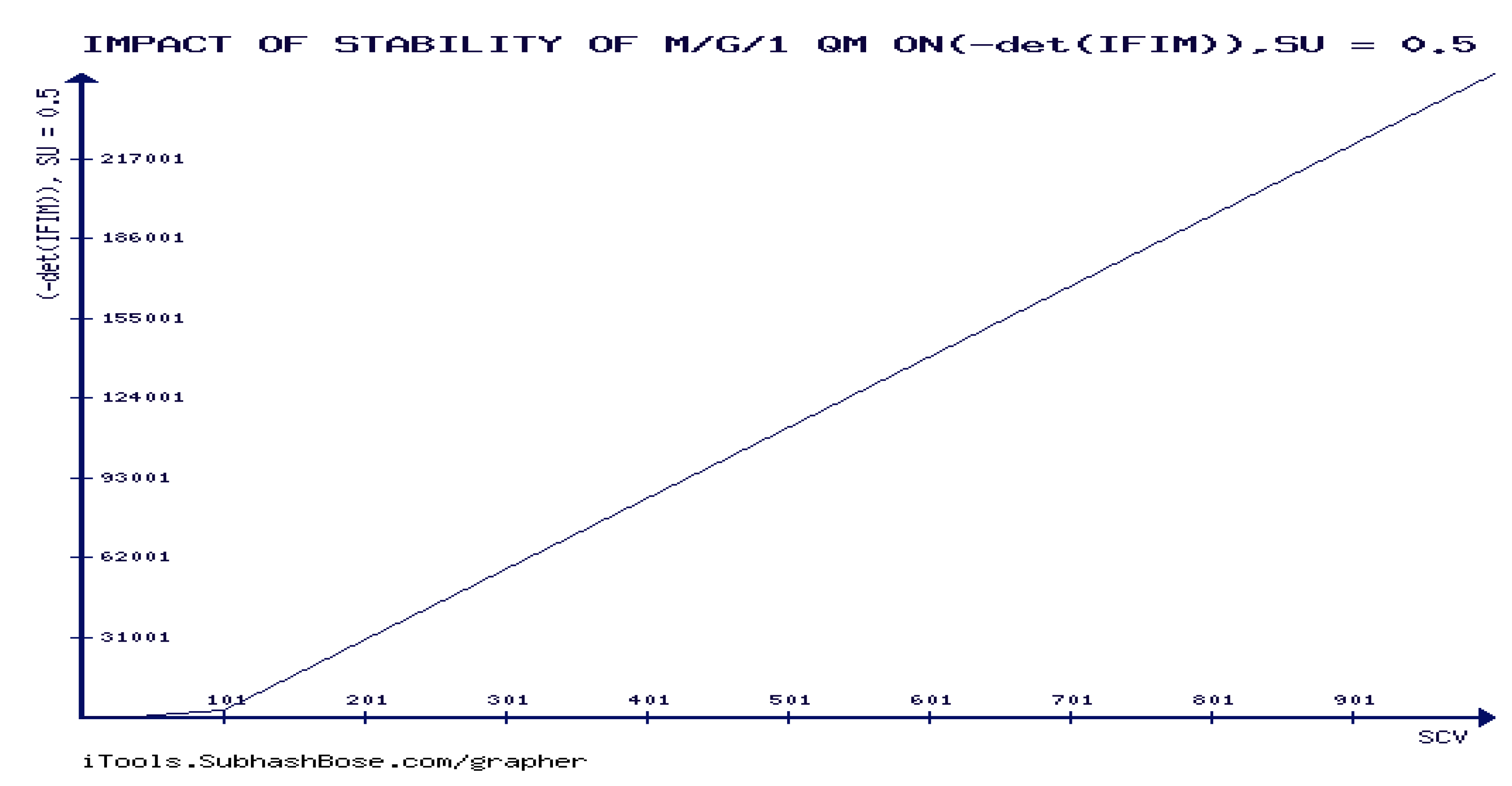
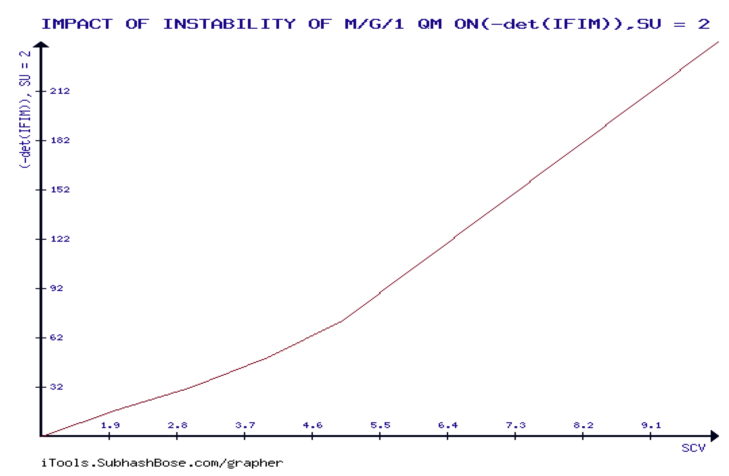
As seen above in Figure 25, det(IFIM) is forever decreasing in SCV if and only if M/G/1 QM is stable.

CASE FOUR:

Δ_{[g^{i j}]} b e h a v i o u r f o r β i n i n s t a b i l i t l y p h a s e o f MG 1 QM, ρ = 2

Figure 26.

As observed in Figure 26, within the instability phase of M/G/1 QM,

β \in (0, 1)

, det(IFIM) is decreasing in

β .

CASE FIVE:

Figure 27.

Figure 27 justifies that the threshold of stability of M/G/1 QM,

ρ = 1

, would be the inflection point of det(IFIM) as well as being the decision parameter which controls the existence of inverse of (IFIM).

Define (QIGUs) by the triad functions, namely

h_{1}^{QIGU}, h_{2}^{QIGU}, h_{3}^{QIGU}

, with

h_{1}^{QIGU}, h_{2}^{QIGU}

: M/G/1 QM

\to [g_{i j}]

, where

[g_{i j}]

(\begin{matrix} \frac{1}{{(1 - ρ)}^{2}} & 0 \\ 0 & \frac{- 1}{{(β + 1)}^{2}} \end{matrix})

(c.f.,(3.3) of Theorem 3.1)

h_{1}^{QIGU} (ρ) = g_{11} = \frac{1}{{(1 - ρ)}^{2}}, ρ \in (0, 1)

(8.55)

h_{2}^{QIGU} (β) = - g_{22} = \frac{1}{{(1 + β)}^{2}}, β \in (1, \infty)

(8.56)

h_{3}^{QIGU} (ρ, β) = \{\begin{matrix} Ψ_{n = 0} (ρ, β) = - l n (1 - ρ), n = 0 \\ Ψ_{n > 0} (ρ, β) = l n (β + 1) - l n (1 - ρ) - l n 2, n > 0 \end{matrix}

(8.57)

provided that

Ψ_{n = 0} (ρ, β), Ψ_{n > 0} (ρ, β)

are determined by (3.7),(3.14) of Theorem 3.1 respectively.

9. Queueing Theoretic Impact on the Continuity of New Devised Queueuing-Information Geometric Unifiers (QIGU)

Theorem 9.1For the stable M/G/1 QM

h_{1}^{QIGU}

is continuous, for

ρ \in (0, 1)

2) h_{1}^{QIGU}

is well-defined.

h_{1}^{QIGU}

is one-to-one.

h_{1}^{QIGU}

is onto.

5) The inverse function of

h_{1}^{QIGU}

is characterized by,

{(h_{1}^{QIGU})}^{- 1} (ρ)

1 - \frac{1}{\sqrt ρ}, ρ \in (0, 1)

h_{2}^{QIGU}

is continuous, for

β \in (1, \infty)

7) h_{2}^{QIGU}

is well-defined.

h_{2}^{QIGU}

is one-to-one.

h_{2}^{QIGU}

is onto.

10) The inverse function of

h_{2}^{QIGU}

is characterized by,

{(h_{2}^{QIGU})}^{- 1} (β)

- 1 + \frac{1}{\sqrt{β}}, β \in (1, \infty) .

11)

Ψ_{n = 0} (ρ, β)

is well defined.

12)

Ψ_{n = 0} (ρ, β)

is continuous if and only if M/G/1 QM is stable.

13)

Ψ_{n = 0} (ρ, β)

is discontinuous

\Leftrightarrow

the instability of the underlying QM is satisfied.

14)

Ψ_{n = 0} (ρ, β)

is one-to-one.

15)

Ψ_{n = 0} (ρ, β)

is onto.

16) The inverse function of

Ψ_{n = 0} (ρ, β)

is characterized by,

{(Ψ_{n = 0} (ρ, β))}^{- 1} (ρ)

1 - e^{- ρ}, ρ \in (0, 1) .

17)

Ψ_{n > 0} (ρ, β)

characterizes a family of non-well defined

(ρ, β) dependent

functions

18)

Ψ_{n > 0} (ρ, β)

is continuous if and only if M/G/1 QM is stable.

19)

Ψ_{n > 0} (ρ, β)

is discontinuous

\Leftrightarrow

the instability of the underlying QM is satisfied.

Proof

1)Let

ρ_{1}, ρ_{2} \in (0, 1)

such that there is a

δ > 0

satisfying

|ρ_{1} - ρ_{2}| < δ

(9.1)

| h_{1}^{QIGU} (ρ_{1}) - h_{1}^{QIGU} (ρ_{2}) | = |\frac{1}{{(1 - ρ_{1})}^{2}} - \frac{1}{{(1 - ρ_{2})}^{2}}| = |\frac{(ρ_{1} - ρ_{2}) (ρ_{1} + ρ_{2} - 2)}{{(1 - ρ_{1})}^{2} {(1 - ρ_{2})}^{2}}| < \frac{δ |(ρ_{1} + ρ_{2} - 2)|}{{(1 - ρ_{1})}^{2} {(1 - ρ_{2})}^{2}} = ε

(9.2)

Clearly by (2.48), the proof 1) follows.

It is also clear that if either

ρ_{1} = 1 or ρ_{2} = 1

. Then, the the underlying QM is unstable, which implies by (9.2), that

ε \to \infty .

This implies that

h_{1}^{QIGU}

is discontinuous at

ρ = 1.

2) Let

ρ_{1}, ρ_{2} \in (0, 1), ρ_{1} \neq ρ_{2} .

Assume that

h_{1}^{QIGU} (ρ_{1}) = h_{1}^{QIGU} (ρ_{2}) .

Hence,

\frac{1}{{(1 - ρ_{1})}^{2}} = \frac{1}{{(1 - ρ_{2})}^{2}}

, equivalently,

{(1 - ρ_{1})}^{2} = {(1 - ρ_{2})}^{2}

. This means,

ρ_{1} = ρ_{2} o r ρ_{1} + ρ_{2} = 2.

We have to reject ,

ρ_{1} = ρ_{2}

. Also,

ρ_{1} + ρ_{2} = 2

is impossible since

ρ_{1}, ρ_{2} \in (0, 1),

Clearly, a contradiction follows. Therefore, 2) holds.

h_{1}^{QIGU} (ρ_{1}) = h_{1}^{QIGU} (ρ_{2})

, then following the same proof as in 2) implies that

ρ_{1} = ρ_{2}

. This proves 3).

4) Obviously, every

ρ \in (0, 1)

uniquely characterizes

\frac{1}{{(1 - ρ)}^{2}}

such that

h_{1}^{QIGU} (ρ)

g_{11} = \frac{1}{{(1 - ρ)}^{2}} .

Hence,

h_{1}^{QIGU}

is onto.

5) Assume

h_{1}^{QIGU} (ρ) = y

. Hence,

{(h_{1}^{QIGU})}^{- 1} (ρ) = 1 - \frac{1}{\sqrt{ρ}}, ρ \in (0, 1)

(9.3)

which proves 5).

6)Let

β_{1}, β_{2} \in (1, \infty)

such that there is a

δ > 0

satisfying

|β_{1} - β_{2}| < δ

(9.4)

| h_{2}^{QIGU} (β_{1}) - h_{2}^{QIGU} (β_{2}) | = |\frac{1}{{(1 + β_{1})}^{2}} - \frac{1}{{(1 + β_{2})}^{2}}| = |\frac{(β_{1} - β_{2}) (β_{1} + β_{2} - 2)}{{(1 + β_{1})}^{2} {(1 + β_{2})}^{2}}| < \frac{δ}{16} |(β_{1} + β_{2} - 2)| = ε

(9.5)

Clearly by (2.48), the proof 6) follows.

7) Let

β_{1}, β_{2} \in (1, \infty), β_{1} \neq β_{2} .

Assume that

h_{2}^{QIGU} (β_{1}) = h_{2}^{QIGU} (β_{2}) .

Hence,

\frac{1}{{(1 + β_{1})}^{2}} = \frac{1}{{(1 + (β_{2})}^{2}}

, equivalently,

{(1 + β_{1})}^{2} = {(1 + β_{2})}^{2}

. This means,

β_{1} = β_{2} o r β_{1} + β_{2} = - 2.

We must reject ,

β_{1} = β_{2}

. Also,

β_{1} + β_{2} = - 2

is impossible since

β_{1}, β_{2} \in (1, \infty),,

Clearly, a contradiction follows. Therefore, 7) holds.

It is also clear that even if the underlying QM is unstable(or equivalently,

β \in (0, 1]

which implies by (9.5), that

ε ↛ \infty) .

This implies that

h_{2}^{QIGU}

is everywhere continuous.

Engaging the same procedure as in 3) and 4), the proofs of 8) and 9) are easily verified respectively.

10)Assume

h_{2}^{QIGU} (β) = \frac{1}{{(1 + β)}^{2}} = w, β \in (1, \infty)

. These leaves one choice,

β = - 1 + \frac{1}{\sqrt w}

(9.6)

This shows that ,

{(h_{2}^{QIGU})}^{- 1} (β)

1 - \frac{1}{\sqrt β}, β \in (1, \infty)

which proves 10).

11)Let

ρ_{1}, ρ_{2} \in (0, 1), ρ_{1} \neq ρ_{2} .

Assume that

Ψ_{n = 0} (ρ_{1}) = Ψ_{n = 0} (ρ_{2}) .

Hence,

- l n (1 - ρ_{1}) = - l n (1 - ρ_{2})

, equivalently,

(1 - ρ_{1}) = (1 - ρ_{2})

. This means,

ρ_{1} = ρ_{2} .

Clearly, a contradiction follows. Therefore, 12) holds.

12) Necessity: Assume that M/G/1 QM is stable, then

ρ_{1}, ρ_{2} \in (0, 1)

Suppose that there is a

δ > 0

satisfying:

|ρ_{1} - ρ_{2}| < δ

(9.7)

| Ψ_{n = 0} (ρ_{1}) - Ψ_{n = 0} (ρ_{2}) | = |\ln (1 - ρ_{1}) - \ln (1 - ρ_{2})|

(9.8)

It is well known that Maclauren’s series of

l n (1 - ρ)

, for

ρ \in (0, 1)

is determined by

l n (1 - ρ) = - \sum_{n = 1}^{\infty} \frac{ρ^{n}}{n} (c . f ., (2.49))

(9.10)

Thus, it follows that

|\ln (1 - ρ_{1}) - \ln (1 - ρ_{2})| < δ \sum_{n = 1}^{\infty} (ρ_{1}^{n - 1} + ρ_{1}^{n - 2} + \dots + 1) = \frac{δ}{(1 - ρ_{1})} = ε

(9.12)

This proves continuity.

Sufficiency:

By (9.12), there exists

\frac{δ_{1}}{(1 - ρ_{1})} = ε_{1} > 0

\frac{δ_{2}}{(1 - ρ_{2})} = ε_{2} > 0

, with

δ = \min (δ_{1}, δ_{2}) > 0

ε = \min (ε_{1}, ε_{2})

satisfying, (9.7) and (9.12). Consequently,

ρ_{1}, ρ_{2} \in (0, 1)

, which directly implies the underlying QM’s stability.

13) Following (9.12), discontinuity of

Ψ_{n = 0}

occurs if and if

ρ_{1} \geq 1

to enforce

ε

to be infinite of any negative real number. Therefore, 13) holds.

The validity of both 14) and 15) can easily be verified.

Assume

Ψ_{n = 0} (ρ) = - l n (1 - ρ) = m, ρ \in (0, 1)

. Thus, it holds that

1 - ρ = e^{- m}

. Consequently,

ρ = 1 - e^{- m}

. This shows that ,

{(Ψ_{n = 0})}^{- 1} (ρ)

1 - e^{- ρ}, ρ \in (0, 1)

, which proves 16).

17) Let

ρ_{1}, ρ_{2} \in (0, 1), (β_{1}, β_{2}) \in (1, \infty) such that ρ_{1} \neq ρ_{2}, β_{1} \neq β_{2}

Assume that

Ψ_{n > 0} (ρ_{1}, β_{1}) = Ψ_{n > 0} (ρ_{2}, β_{2}) .

Hence,

\frac{(β_{1} + 1)}{(1 - ρ_{1})} = \frac{(β_{2} + 1)}{(1 - ρ_{2})}

. This means,

(β_{1} - β_{2}) + (ρ_{1} - ρ_{2}) = (β_{2} ρ_{1} - β_{1} ρ_{2})

(9.13)

By (9.13), 17) holds.

It is obvious that

Ψ_{n > 0}

is continuous for all

β \in (1, \infty), ρ \in (0, 1)

. This proves the necessity requirement. As for the sufficiency requirement, let

Ψ_{n > 0} (ρ, β)

be continuous. This directly implies that

l n (1 - ρ)

attains non- infinite real values. Consequently,

1 - ρ > 0

. Hence, the underlying M/G/1 QM is stable. This proves 18).

To prove 19), it is clear that

Ψ_{n > 0} (ρ, β)

is discontinuous if and only if both

l n (β + 1) and \ln (1 - ρ)

is discontinuous. This is equivalent to

β > - 1, ρ \geq 1

. Equivalently, M/G/1 QM is unstable.

10. Closing Remarks with Next Phase Research

This paper discusses the application of information geometric concepts in queueing theory, specifically focusing on the specified QM. It introduces the Fisher information metric, the 𝛼-connection, and analyses the geometric properties of the queue manifold, such as Gaussian and Ricci curvatures. The paper also highlights the potential for further research in IG unification with existent knowledge of scientific fields.

References

Mageed IA, Yuyang Zhou, Y, Liu, Y, and Zhang Q(a), “ Towards a Revolutionary Info-Geometric Control Theory with Potential Applications of Fokker Planck Kolmogorov(FPK) Equation to System Control, Modelling and Simulation”,In2023 28th International Conference on Automation and Computing (ICAC) 2023, 30th Aug- Sep 1. IEEE.
Mageed IA, Yuyang Zhou, Y, Liu, Y, and Zhang Q(b), “Z_ab of the Stable Five-Dimensional M/G/1 Queue Manifold Formalism’s Info- Geometric Structure with Potential Info-Geometric Applications to Human Computer Collaborations and Digital Twins”,In2023 28th International Conference on Automation and Computing (ICAC) 2023, 30th Aug- Sep 1. IEEE.
Mageed, I.A, Info-Geometric Analysis of Gamma Distribution Manifold with Gamma Distribution Impact to Advance Satellite Earth Observations, The 2nd International Conference on Applied Mathematics, Informatics, and Computing Sciences (AMICS 2023), Ghent University, Belgium.
A. Mageed, Q. Zhang, T. C. Akinci, M. Yilmaz and M. S. Sidhu, “Towards Abel Prize: The Generalized Brownian Motion Manifold’s Fisher Information Matrix With Info-Geometric Applications to Energy Works,” 2022 Global Energy Conference (GEC), Batman, Turkey, 2022, pp. 379-384. [CrossRef]
Mageed, I.A, Info-Geometric Analysis of Gamma Distribution Manifold with Gamma Distribution Impact to Advance Satellite Earth Observations, The 2nd International Conference on Applied Mathematics, Informatics, and Computing Sciences (AMICS 2023), Ghent University, Belgium.
A Mageed, D.I. Info- Geometric Analysis of the Stable G/G/1 Queue Manifold Dynamics With G/G/1 Queue Applications to E-health. Preprints 2024, 2024011813. [CrossRef]
I.A. Mageed, and D.D. Kouvatsos, The Impact of Information Geometry on the Analysis of the Stable M/G/1 Queue Manifold. In Proceedings of the 10th International Conference on Operations Research and Enterprise Systems—Volume 1: ICORES, ISBN 978-989-758-485-5, 2021, p. 153-160. [CrossRef]
I.A. Mageed, and Kouvatsos, D.D., 2019, Information Geometric Structure of Stable M/G/1 Queue Manifold and its Matrix Exponential, Proceedings of the 35th UK Performance Engineering Workshop, School of Computing, University of Leeds, Edited by Karim Djemame, 16^th of Dec.2019, p.123-135. [Online] at: https://sites.google.com/view/ukpew2019/home.
MIT Open Course Ware,2010. Online available at: https://ocw.mit.edu/courses/mathematics/18-02sc-multivariable-calculus-fall-2010/4.-triple-integrals-and-surface-integrals-in-3-space/part-b-flux-and-the-divergence-theorem/session-84-divergence-theorem/MIT18_02SC_MNotes_v10.1.pdf.
A Mageed, D.I. On the Rényi Entropy Functional, Tsallis Distributions and Lévy Stable Distributions. Preprints 2024, 2024011996. https://doi.org/10.20944/preprints202401.1996.v1.
Grivel, E., Diversi, R., & Merchan, F. (2021). Kullback-Leibler and Rényi divergence rate for Gaussian stationary ARMA processes comparison. Digital Signal Processing, 116, 103089.
Cai, T. T., Guo, Z., & Ma, R. (2023). Statistical inference for high-dimensional generalized linear models with binary outcomes. Journal of the American Statistical Association, 118(542), 1319-1332.
Marmin, A., de Morais Goulart, J. H., & Févotte, C. (2023). Majorization-minimization for Sparse Nonnegative Matrix Factorization with the β-divergence. IEEE Transactions on Signal Processing.
Cilingir, K., Manzelli, R., Kulis,B., 2020, Deep Divergence Learning. Online available at; arXiv:2005.02612v1.
Chow, B., Lu, P., & Ni, L. (2023). Hamilton’s Ricci flow (Vol. 77). American Mathematical Society, Science Press.
Gilkey, P., Brozos-Vazquez, M., Garcia-Rio, E., Nikčević, S., & Vásquez-Lorenzo, R. (2022). The geometry of Walker manifolds. Springer Nature.
Bachmann, Gregor, Gary Bécigneul, and Octavian Ganea. “Constant curvature graph convolutional networks.” In International conference on machine learning, pp. 486-496. PMLR, 2020.
Sun, Ao. “Compactness of constant mean curvature surfaces in a three-manifold with positive Ricci curvature.” Pacific Journal of Mathematics 305, no. 2 (2020): 735-756.
Meyer, Carl D., and Ian Stewart. Matrix analysis and applied linear algebra. Society for Industrial and Applied Mathematics, 2023.
Zhang, Yuzhe, and Jianmin Zheng. “An Overview of Developable Surfaces in Geometric Modeling.” Recent Patents on Engineering 16, no. 5 (2022): 87-103.
Kamarudzaman, Anis Solehah Mohd, Nurul Huda Mohamad Nasir, and Md Yushalify Misro. “Gaussian and Mean Curvature of Biquintic Trigonometric Bézier Surface.” Pertanika Journal of Science & Technology 30, no. 2 (2022).
Wang, Jianchao, Huilin Xing, Zongwei Jin, Yuyang Tan, Shuo Pang, and Junbiao Liu. “3D geometric modelling of the Northwest Pacific slabs: A review and new high-precision model.” Earth-Science Reviews (2023): 104351.
Banica, Teo. “Calculus and applications.” arXiv preprint arXiv:2401.00911 (2024).
Latayada, Mary Joy R. “On the Number of Restricted One-to-One and Onto Functons Having Integral Coordinates.” European Journal of Pure and Applied Mathematics 16, no. 4 (2023): 2751-2762.
Irving, Ron. Beyond the quadratic formula. Vol. 62. American Mathematical Soc., 2020.
Mageed, I. A., & Zhang, Q. (2023). Threshold Theorems for the Tsallisian and Rényian (TR) Cumulative Distribution Functions (CDFs) of the Heavy-Tailed Stable M/G/1 Queue with Tsallisian and Rényian Entropic Applications to Satellite Images (SIs). electronic Journal of Computer Science and Information Technology, 9(1), 41-47.
Roussel, M., R., April 2019, Stability Analysis for ODEs, Morgan & Claypool Publishers.
Schloss, James, Peter Barnett, Rashi Sachdeva, and Thomas Busch. “Controlled creation of three-dimensional vortex structures in Bose-Einstein condensates using artificial magnetic fields.” Physical Review A 102, no. 4 (2020): 043325.
Bailes, Matthew, Beverly K. Berger, P. R. Brady, M. Branchesi, Karsten Danzmann, M. Evans, Kelly Holley-Bockelmann et al. “Gravitational-wave physics and astronomy in the 2020s and 2030s.” Nature Reviews Physics 3, no. 5 (2021): 344-366.
Dawkins, P., 2021, Paul’s Online Notes, web source. Online available at: https://tutorial.math.lamar.edu.
Breneman, James E., Chittaranjan Sahay, and Elmer E. Lewis. Introduction to reliability engineering. John Wiley & Sons, 2022.
A. Mageed and Q. Zhang, “An Information Theoretic Unified Global Theory For a Stable M/G/1 Queue With Potential Maximum Entropy Applications to Energy Works,” 2022 Global Energy Conference (GEC), Batman, Turkey, 2022, pp. 300-305. [CrossRef]

Figure 1. SM’s parametrization [3].

Figure 2. curved surfaces’ geodesic representation [6].

Figure 8. (c.f., [21]).

Figure 9. Catenoid (c.f., [21]).

Disclaimer/Publisher’s Note: The statements, opinions and data contained in all publications are solely those of the individual author(s) and contributor(s) and not of MDPI and/or the editor(s). MDPI and/or the editor(s) disclaim responsibility for any injury to people or property resulting from any ideas, methods, instructions or products referred to in the content.

© 2024 by the authors. Licensee MDPI, Basel, Switzerland. This article is an open access article distributed under the terms and conditions of the Creative Commons Attribution (CC BY) license (http://creativecommons.org/licenses/by/4.0/).

Copyright: This open access article is published under a Creative Commons CC BY 4.0 license, which permit the free download, distribution, and reuse, provided that the author and preprint are cited in any reuse.

MDPI Initiatives

Important Links

Choose an area of interest and we will send you notifications of new preprints at your preferred frequency.

Disclaimer

Towards An Info-Geometric Theory Of The Analysis Of Non-Time Dependent Queueing Systems

Abstract

1. Introduction

2. Main Definitions

2.1. Main Definition on IG

2.2. Gaussian and Mean Curvatures, KGand H respectively (c.f., [21])

2.3. Different Approach to Gaussian and Mean Curvatures (Angular Technique) (c.f., [22])

2.4. Well Defined Functions and Bijective Functions

2.5. Stability Analysis for Ordinary Differential Equations (ODEs) [27]

2.6. Scalar Curvature(Ricci Scalar), R and Einestein Tensor, ℘

2.7. Maxima and Minima of Functions of Two Variables [30]

2.8. Continuous Functions (c.f., [31])

2.9. The Maclauren’s Series of l n 1 − x for x a r o u n d z e r o (Shaw,2015)

3. The Fim and Its Inverse for the Stable M/G/1 QM

4. The α(. OR ∇ α )-Connection of the M/G/1 QM

5. Variational Inference, KD,JD,RÉNYI AND s AB DIVERGENCES OF STABLE M/G/1 QM

5.1. KD and JD Divergences of Stable M/G/1 QM

5.2. Rényi Divergence of Stable M/G/1 QM

5.3. sAB divergence, D s , A B η , γ (p||q) of Stable M/G/1 QM

6. Investigations of the Developability of the Stable M/G/1 QM ,RICCI CURVATURE (RCT) tENSOR and QT-IG Unifiers

6.1. Investigation of Developability of M/G/1 QM and Finding Its Ricci Curvature Tensor (RCT)

6.2. Revealing Novel QT-IG Unifiers and Discovering Their Algebraic Structures

7. eFIM(M/G/1) & Impact of Stability of M/G/1 QM on the Stability of Fim

7.1 Exponential Matrix of FIM

7.2. Impact of Stability of M/D/1 QM on the stability of FIM

7.3. Revealing Queue-Fisher Information Matrix Unifiers, (QFIMU)

9. Queueing Theoretic Impact on the Continuity of New Devised Queueuing-Information Geometric Unifiers (QIGU)

10. Closing Remarks with Next Phase Research

References

MDPI Initiatives

Important Links

Subscribe

2.2. Gaussian and Mean Curvatures, K_Gand H respectively (c.f., [21])

2.6. Scalar Curvature(Ricci Scalar), $R$ and Einestein Tensor, $℘$

2.9. The Maclauren’s Series of $l n (1 - x)$ for $x a r o u n d z e r o$ (Shaw,2015)

4. The α(. OR $\nabla^{(α)}$ )-Connection of the M/G/1 QM

5.3. sAB divergence, $D_{s, A B}^{η, γ}$ (p||q) of Stable M/G/1 QM

7. e^FIM(M/G/1) & Impact of Stability of M/G/1 QM on the Stability of Fim