Preprint
Article

Bayesian Feature Extraction for Two-Part Latent Variable Model with Polytomous Manifestations

Altmetrics

Downloads

146

Views

42

Comments

0

A peer-reviewed article of this preprint also exists.

This version is not peer-reviewed

Submitted:

31 January 2024

Posted:

01 February 2024

You are already at the latest version

Alerts
Abstract
Semi-continuous data are very common in the social science and economics. In this paper, a Bayesian variable selection procedure is developed to assess the influence of exogenous factors including observed and unobserved on the semi-continuous data. Our formulation is based on the two-part latent variable model with polytomous response. We consider two schemes for the penalties of regression coefficients and factor loadings: the Bayesian spike and slab bimodal prior and the Bayesian lasso prior. Within the Bayesian framework, we implement Markov Chains Monte Carlo sampling method to conduct posterior inference. To facilitate posterior sampling, we recast the logistic model in part one as the norm-like mixture model. Gibbs sampler is designed to draw observations from the posterior. Our empirical results show that with suitable hyper-parameters, the spike and slab bimodal method slightly outperforms the Bayesian lasso in the current analysis. Finally, a real example related to the China household finance survey is analyzed to illustrate the application of the methodology.. .
Keywords: 
Subject: Business, Economics and Management  -   Econometrics and Statistics

MSC:  62H12; 62F15

1. Introduction

Semi-continuous data, characterized by excessive zeros, are very common in the fields of social science and economics. A typical example is given by [1] in the analysis of medical expenditures, in which the zeros correspond to a subpopulation of patients who do not use health services, while the positive values describe the actual levels of expenditures in use among users. In understanding such type of data structure, two-part model [2] is a widely appreciated statistical method. The basic assumption on two-part model is that the overall model is consisted of two processes: one binary process (Part one) and one continuous positive-valued process (Part two). The binary process, usually formulated within the logistic or probit regression model, is used to indicate whether the items are responded or not, while the continuous process, conditioning on the binary process, is used to describe what the actual levels of responses are (see, e.g., [3]). By combining two processes into one, two-part model provides a unified and flexible way in describing various relevance underlying semi-continuous data. Now, two-part model has been widely used in the health service [4,5,6], the medical expenditures [1,7,8,9], the household finance [10], the substance use study [11,12] and the genome analysis [13].
The traditional two-part model usually formulates the exogenous explanatory factors as fixed and observed. However, in the real applications especially in the social survey, many unobserved/latent and random factors also have important impacts on the outcome variable. This fact is revealed by [14] in the study of children’s aggressive behavior. [14] noted that two factors, the propensity to engage in aggressive behavior and the propensity to have high aggressive activity levels, had significant influence on the children’s aggressive behavior. They incorporated such two latent factors into analysis and established a two-component-two-part mixture model to identify the heterogeneity of population; [15] noticed that in China, the finance literacy of a family had a nonignorable influence on the desire to holding finance debts, and also affected the amount of finance debt being held. They suggested conducting a joint analysis of latent factor and observed covariates in two-part regression model. The latent factor is further manifested by multiple binary measurements via factor analysis model. [16] incorporated two-part regression model into the general latent variable model framework and analyzed the internal relationships between multiple factors longitudinally. These methods have brought significant attention to the two-part model in behavioral science, economics, psychology, and medicine in recent years, see for example, [13,17,18] and references therein for further developments of two-part model.
In the analysis of semi-continuous data, an important issue is to determine which explanatory factor is helpful in improving model fit. This issue is especially true when the number of exogenous factors is large since the commonly used forward and backward regression procedure is extremely time-consuming. Now, lasso and its extensions [19,20,21,22,23,24,25,26] have been the most commonly used methods for the feature extraction. A typical feature of these methods is to put some suitable penalties on the coefficients and shrink many coefficients to zero, thus performing variable selection. Recently, these penalization/regularizatio approaches have been applied widely for prediction and prognosis (see for example, [27,28]). Though more appealing, the lasso-type regularization also suffers some limitations. For example, most contributions are developed within the frequency framework and the performance heavily depends on the large sample theory. It also readily leads to computational difficulty in the analysis of mixed data. An alternative for the variable selection is conducted within the Bayesian framework. Statisticians have introduced hierarchical models with mixture spike-and-slab priors that can adaptively determine the amount of shrinkage [29,30]. The spike-and-slab prior is the fundamental basis for most Bayesian variable selection approaches, and has proved remarkably successful [29,30,31,32,33,34,35]. Recently, Bayesian spike-and-slab priors have been applied to predictive modeling and variable selection in large scale genomic studies, see [36] for a simple review. Nevertheless, model selection has never been considered in the two-part regression model with latent variables. In this study, we introduce spike and slab model and Bayesian lasso into two-part latent variable model, which is the first attempt for this model.
Our formulation is more along with the lines of spike and slab bimodal prior in [33] and Bayesian Lasso in [37]. We formulate the problem by specifying a normal distribution with mean zero to the regression coefficient or factor loading of interest. The probability of a related variable being excluded or included is governed by the variance. To model the shrinkage of coefficients properly, we consider two schemes for the variance parameter: one is the two-point mixture model with one component located at the point close to zero and the other component situated at the point far away zero. The proportion is governed by a beta-distribution with suitable hyperparameters. Another scheme is along with the Bayesian lasso in which the variance is specified via a gamma distribution scaled by the penalty parameters. Two schemes are unified into a hierarchical mixture model. Within the Bayes paradigm, we developed a fully Bayesian selection procedure for the two-part latent variable model. We resort to the Markov Chains Monte Carlo sampling method. Gibbs sampler is used to draw observations from the posterior. We obtained all full conditionals. Posterior analysis is carried out based on the simulated observations. We investigate the performance of the proposed methods via simulation study and a real example. Our empirical results show that two schemes results in similar results in the variable selection but SS with suitable hyperparameters slightly outperforms over BaLsso in the correct rate.
The remainder of this paper is organized as follows. Section 2 introduces the proposed model for the semi-continuous data with latent variables. Section 3 develops the MCMC algorithm for the proposed model. Bayesian inference procedures including parameters estimation and model assessment are also presented in this section. In Section 4, we present the results of simulation study to assess the performance of our proposed methodology and illustrate the practical value of our proposed model with household finance debt data. Section 5 concludes the paper with a discussion. Some technical details are given in the Appendix.

2. Model Description

In Section 2.1, a basic formulation for analyzing semi-continuous data with latent variables is presented. Section 2.2 presents a Bayesian procedure for the feature extraction.

2.1. Two-Part Latent Variable Model

Suppose that for i = 1 , 2 , , n , s i is a semicontinuous outcome variable which takes value in [ 0 , ) ; x i is a generic vector consisted of r fixed covariates representing the collection of observed explanatory factors of interest. We assume that each x i j in x i is standardized in the sense i = 1 n x i j = 0 and i = 1 n x i j 2 = 1 for j = 1 , , r . Moreover, we include m letent/unobserved variables ω i = ( ω i 1 , , ω i m ) T into analysis to account for unobserved heterogeneity of responses.Conceptually,these latent variables can be the covariates that are not directly observed or the synthesization of some highly correlated explanatory items suffering from the noisy. Inclusion of latent variables can improve model fits and strengthen the power of model interpretation, see [38] for more discussions on the latent variables in a general setting. To deal with the spike of s i at zero, we follow the common routine in literature (see for example, [9,11]) and identify s i with two surrogate variables: u i = I { s i > 0 } and z i = log ( s i + ) , where I ( A ) denotes the indicator function of set A and a + represents the positive part of a. That is, we separate the whole dataset into two parts: one part is the binary dataset which corresponds to the response-to-nonresponse indicators of subject and the other part is the logarithm of positive values. Our interest focuses on the exploration of effects of exogenous factors on two parts.
We assume that u i and z i satisfy the following sampling models:
p ( u i | x i , ω i ) = exp ( u i η i u ) 1 + exp ( η i u ) , η i u = α + β x T x i + β ω T ω i ,
p ( z i | u i = 1 , ω i ) = N ( η i z , σ 2 ) , η i z = γ + ψ x T x i + ψ ω T ω i ,
in which α and γ are the intercept parameters, β x and ψ x are the vectors of regression coefficients, and β ω and ψ ω are the vectors of factor loadings; σ 2 is the scale and `T’ is the transpose operator of vector or matrix; For compactness, we write β = ( β x T , β ω T ) T and ψ = ( ψ x T , ψ ω T ) T and treat w i = ( x i T , ω i T ) T as the complete explanatory variables.
The involvement of latent variables apparently complicates the model. It readily results in model identification problem [39,40]. This is especially true when the dimension of ω i is high. In this case, any auxiliary information is required to manifest ω i further. Among various-easy-constructs, we consider latent variable (LV, [39,40]) approach. A basic assumption on LV approach is that there exist, say p manifestations y i = ( y i 1 , , y i p ) T , of which each y i j may be continuous, counted or categorical, and assuming that they satisfy the following link equation
F ( y i , ω i , ϵ i , φ ) = 0 ,
where F is a known and fixed link function, ϵ i is the vector of errors used to identity the idiosyncratic part of y i that can not be explained by ω i , and φ is the vector of unknown parameters used to quantify the uncertainty of model. The information about ω i is manifested by y i via F. In this paper, in view of the real applications, we consider p ordered categorical variable y i = ( y i 1 , , y i p ) T , of which y i j takes value in { 0 , 1 , , c j } ( c j > 1 ) and satisfies the following link model:
y i j = j if δ j j < y i j * δ j , j + 1 ,
where δ j 0 < δ j 1 < < δ j c j < δ j , c j + 1 are the threshold parameters with δ j 0 = and δ j , c j + 1 = + , and y i * = ( y i 1 * , , y i p * ) T is the vector of latent responses satisfying the factor analytic model:
y i * = μ + Λ ω i + ϵ i ,
ω i i i d . N m [ 0 , Φ ] , ϵ i N p [ 0 , I p ] , and ω i ϵ i ,
where μ is a p-dimensional intercept vector, Λ is the p × m -dimensional factor loading matrix, and I p is the identity matrix of order p. We assume that conditional upon ω i , s i and y i are independent.
We refer to the model specified by (1), (2) and (4) associated with (5) as the two-part latent variable model with polytomous responses. It provides a unified framework to explore the dependence of binary, continuous and categorical data simultaneously. The dependence between them results from the share of common factors or latent variables. If ω i is degenerated at zeros or the factor loadings are taken as zeros, the dependence among them disappears, and the overall model reduces to the traditional two-part model and ordinal regression model.
To facilitate the efficient calculation, motivated by the key identity in [41] (see squation (2) in their seminar paper), we express the logistics model (1) as the mixture model of form
exp ( u i ( α + β T w i ) ) 1 + exp ( α + β T w i ) = 2 1 exp ( κ i ( α + β T w i ) ) 0 exp u i * 2 ( α + β T w i ) 2 p P G ( u i * ) d u i * ,
where κ i = u i 0.5 , and p P G ( u ) is the standard Pólya-Gamma probability density function. Assuming that we introduce auxiliary variables u i * and augment them with u i , then equation (1) can be considered as the marginal density of the joint distribution
p ( u i , u i * x i , ω i ) = 2 1 exp κ i η i u u i * 2 η i u 2 p P G ( u i * ) .
Note that the exponential part in the brackets is the kernel of normal density function with respect to η i u . Hence, it admits conjugate full-conditional distributions for all regression coefficients, factor loadings and factor variables, leading to a straightforward Bayesian computation.
Let U = { u i } i = 1 n , Z = { z i } i = 1 n ,and Y = { y i } i = 1 n be the sets of observed variables; We write Ω = { ω i } i = 1 n for the collect of factor variables, and write U * = { u i * } i = 1 n , V * = { v i * } i = 1 n , Y * = { y i * } i = 1 n for the sets of latent response variables. The complete-data likelihood is given by
p ( U , U * , Z , V * , Y , Y * , Ω | θ ) = p ( U , U * | Ω , α , β ) p ( Z , V * | U , Ω , γ , ψ , σ 2 ) p ( Y | Y * , δ ) p ( Y * | Ω , μ , Λ ) p ( Ω | Φ ) = i = 1 n exp κ i η i u 1 2 u i * ( η i u ) 2 p P G ( u i * | 1 , 0 ) × i I 1 2 π σ exp 1 2 σ 2 ( z i η i z ) 2 × i = 1 n j = 1 p = 0 c j I { δ j < y i j * δ j , + 1 , y i j = } × i = 1 n j = 1 p 1 2 π exp 1 2 ( y i j * μ j Λ j T ω i ) 2 × i = 1 n 1 ( 2 π ) m | Φ | 1 / 2 exp 1 2 t r [ Φ 1 ω i ω i T ] .
where I = { i : u i = 1 } is the set of indices, δ = { δ j } is the set of threshold parametes, and θ = { α , β , γ , ψ , σ 2 , μ , Λ , Φ , δ } is the vector of unknown parameters. For the moment, we assume θ j in θ all are free.

2.2. Bayesian Feature Selection

Generally speaking, regression variables x i and factor variables ω i may not have impacts on the u i and z i simultaneously, and some redundant variables may exist. The presence of redundant variables not only decreases the model fit but also weakens the power of model interpretation. Therefore, it is necessary to determine which regression coefficient or factor loading is significantly away from zero. In the context of frequency statistics, this issue is generally tackled out via stepwise regression, in which each variable is decided to be exclude or included according to the model fit. However, the situation becomes complex when the number of independent variables is large. In this paper, we pursuit a Bayesian variable selection procedure. To this end, we follow [37] and assume
β N q ( 0 , d i a g { γ β k 2 } ) , ψ N q ( 0 , σ 2 d i a g { γ ψ k 2 } ) ,
in which we use d i a g { a k } to represent a diagonal matrix with the k t h diagonal element a k and let q = r + m . That is, we assume that each β k in β ( ψ k is similar) is centered at zero (or equivalently each w i k is excluded from w i ) but with the probability governed by the variance γ β k 2 . If γ β k 2 is close to zero, then the probability of β k taking zero increases, and w i k tends to be excluded; conversely, if γ β k 2 is large, then the probability of β k being zero is small and w i k tends to be maintained. As a result, the value of γ β k 2 plays a key role in determining whether w k is relevant to be selected in Part one. With this in mind, a reasonable assumption on γ β k 2 and γ ψ k 2 is that:
γ β k 2 i n d . ( 1 w β ) δ ν β 0 η β k 2 ( · ) + w β δ η β k 2 ( · ) ,
γ ψ k 2 i n d . ( 1 w ψ ) δ ν ψ 0 η ψ k 2 ( · ) + w ψ δ η ψ k 2 ( · ) ,
where δ a ( · ) is the Dirac measure concentrated at point a, w β is the random weight used to measure the similarity between γ β k 2 and η β k 2 , and η β k 2 is the hyperparameter used to represent how far β k is away from zero or slab; ν β 0 is a previously specified small positive value used to identity the `spike’ of β k at zero. In other words, every γ β k 2 is assumed to be equal to η β k 2 with probability w β and equal to ν β 0 η β k 2 with probability 1 w β . This is also true for w ψ , η ψ k and ν ψ 0 . To model w β and w ψ properly, we assign the following beta distributions to them
p ( w β | a β , b β ) = B e t a ( a β , b β ) , p ( w ψ | a ψ , b ψ ) = B e t a ( a ψ , b ψ ) ,
where a β , a ψ , b β and b ψ are the hyperparameters used to control the shape of beta density, that is, to determine the magnitude of weights in ( 0 , 1 ) . For example, if a β 1 in equation (12) is small and b β 1 is large, then equation (12) encourages w β to take small value with high probability. In contrast, it follows from 1 B e t a ( a β , b β ) = B e t a ( b β , a β ) that large a β 1 and small b β 1 encourage w β to take large value in ( 0 , 1 ) . In the case that a β 1 = b β 1 = 1.0 , equation (12) reduces to the uniform distributions on ( 0 , 1 ) . In this case, every value in ( 0 , 1 ) is possible for w β with the same probability. In the real applications, if no information can be available, one can assign the values to them to ensure the beta distribution to be inflated enough.
Finally, to measure the magnitudes of `slap’ in the distributions of β k and ψ k , we specify gamma distributions for η β k 2 and η ψ k 2 , or equivalently,
η β k 2 | a β 1 , a β 2 i i d . I G ( τ β 0 , ζ β 0 ) , η ψ k 2 | a ψ 1 , a ψ 2 i i d . I G ( τ ψ 0 , ζ ψ 0 ) ,
where ` I G ( a , b ) ’ denotes the inverse-gamma distribution with mean b / ( a 1 ) for a > 1 and variance b 2 / ( ( a 1 ) 2 ( a 2 ) ) for a > 2 ; τ β 0 , ζ β 0 , τ ψ 0 and ζ ψ 0 are the hyperparameters which are treated to fixed and known. Similarly, one can assign values to them to ensure (13) to be dispered enough. For example, we can follow the routine in [33] in the ordinary regression analysis, and set τ β 0 = τ ψ 0 = 1.0 and ζ β 0 = ζ ψ 0 = 0.05 to obtain dispersed priors.
Note that equations (10) and (11) can be formulated as hierarchy as follows: for k = 1 , , q ,
γ β k 2 = f β k η β k 2 , γ ψ k 2 = f ψ k η β k 2 ,
f β k | ν β 0 , ω β i i d . ( 1 w β ) δ v β 0 ( · ) + w β δ 1 ( · ) ,
f ψ k | ν ψ 0 , w ψ i i d . ( 1 w ψ ) δ v ψ 0 ( · ) + w ψ δ 1 ( · ) ,
where f β k and f ψ k are the latent binary variables respectively. Such a formulation aims to separate η β k 2 and η ψ k 2 from the distributions (10) and (11) to facilitate posterior sampling.
It is instructive to compare the proposed method to the Bayesian lasso [37], in which the variance parameters γ β k 2 and γ ψ k 2 in equation (9) are specified via exponential distributions as follows:
p ( γ β 2 λ β 2 ) = k = 1 q λ β k 2 2 exp ( λ β k 2 γ β k 2 / 2 ) ,
p ( γ ψ 2 λ ψ 2 ) = k = 1 q λ ψ k 2 2 exp ( λ ψ k 2 γ ψ k 2 / 2 ) ,
where λ β 2 = ( λ β 1 2 , , λ β q 2 ) T and λ ψ 2 = ( λ ψ 1 2 , , λ ψ q 2 ) T λ ψ k 2 are the shrinkage/penality parameters used to control the amount of shrinkage of β k and ψ k toward zero.
Modeling γ β k 2 and γ ψ k 2 like equations (16) and (17) lead to marginal distributions of β k and ψ k as the laplace distributions with location zero and scale λ k . The penalty parameters λ β k 2 and λ ψ k 2 are rather crucial in determining the amount of shrinkage of parameters. Figure 1 presents the plots of densities of Laplace distribution L A ( λ ) ( λ > 0 ) across various choices of λ . It can be seen that the larger the value of γ , the more kurtosis the density, indicating more penalties on the regression coefficient.
Due to their key role in equations (16) and (17), for λ β 2 and λ ψ 2 , we assign the following gamma priors to them, i.e.,
p ( λ β 2 ) = k = 1 q p ( λ β k 2 ) = k = 1 q G a ( a k 0 , b k 0 ) ,
p ( λ ψ 2 ) = k = 1 q p ( λ ψ k 2 ) = k = 1 q G a ( c k 0 , d k 0 ) ,
where ` G a ( ν , λ ) ’ denotes the gamma distribution with mean ν / λ . As the previous discussions, the values of a k 0 , b k 0 , c k 0 and d k 0 should be selected with care since they relate the shrinkages directly. Similar to that in (13), one can set a k 0 = c k 0 = 1 , b k 0 = d k 0 = 0.05 to enhance the robustness of inference. This routine is followed in our empirical study.
Let F β * = { f β k } , F ψ * = { f ψ k } , γ β 2 = { γ β k 2 } , γ ψ 2 = { γ ψ k 2 } , η β 2 = { η β k 2 } , η ψ 2 = { η ψ k 2 } . We treat ν β 0 and ν ψ 0 as known hyperparameters. Note that γ β 2 and γ ψ 2 are totally determined by F β * , F ψ * and η β 2 , η ψ 2 . In the following, we abbreviate spike and slab bimodal prior to SS and Bayesian lasso to BaLsso.

3. Bayesian Inference

3.1. Prior Specification and MCMC Sampling

In view of the model complexity, we consider Bayesian inference. Some priors are required to specify for unknown parameters to complete Bayesian model specification. Based on the model convention, it is naturally to assume that the parameters involved in the different models are independent.
Firstly, for μ , Λ and Φ , we consider the following conjugate priors:
p ( μ ) = N p ( μ 0 , Σ 0 ) ,
p ( Λ ) = k = 1 p p ( Λ k ) = k = 1 p N m ( Λ 0 k , H 0 k ) ,
p ( Φ ) = I W ( ρ 0 , R 0 1 ) ,
where ` I W ( ρ , R ) ’ denotes the inverse Wishart distribution with degrees of freedom ρ and scale matrix R [42]; Λ k T is the k t h row vector of Λ ; μ 0 , Σ 0 ( p × p ) > 0 , Λ 0 k , H 0 k ( m × m ) > 0 , ρ 0 > 0 , and R 0 ( m × m ) > 0 are the hyperparameters which are treated to be fixed and known.
Secondly, for α , γ , σ 2 in part one and two, we assume they are mutually independent and satisfy
p ( α ) = N ( α 0 , σ α 0 2 ) , p ( γ ) = N ( γ 0 , σ γ 0 2 ) , p ( σ 2 ) G a ( a 0 , b 0 ) ,
where α 0 , σ α 0 2 , γ 0 , σ γ 0 2 and a 0 , b 0 are the fixed hyperparameters.
Lastly, for threshold parameter δ , without loss of generality, we assume that c j , the number of categories of y i j , is invariant across the subscript j and equals to c. Moreover, we assume that p ( δ ) = j = 1 p p ( δ j ) , where δ j = ( δ j k ) is the j t h row vector of δ . In the following, we suppress the subscript j in δ j k for notational simplicity and write δ for δ j .
Let F 0 ( · ) be any strictly monotonically increasing and differentiable function on R with F 0 ( + ) = 1 and F 0 ( ) = 0 . For example, one can take F 0 = Φ ( · / τ 0 ) for some τ 0 > 0 or student distribution with degrees of freedom ν 0 , where Φ ( · ) is the standard normal distribution function. To specify a prior for δ , we follow [43] and let p j = F 0 ( δ j ) F 0 ( δ j 1 ) for j = 1 , , c . It is easily to show that the transformation is invertible with Jacobi determination unity. We first consider the following Dirichlet distribution for p = ( p 1 , , p c ) T :
π ( p ) = 1 B ( η 1 , , η c + 1 ) p 1 η 1 1 p c η c 1 ( 1 = 1 c p ) η c + 1 1
where B ( η 1 , , η c + 1 ) = j = 1 c + 1 Γ ( η j ) / Γ ( j = 1 c + 1 η j ) is the multivariate beta function evaluated at η 1 , , η c + 1 , and η j > 0 . Then, by the formula of inverse transformation, the joint distribution of δ is given by
π ( δ ) = 1 B ( η 1 , , η c + 1 ) p 1 η 1 1 p c η c 1 ( 1 = 1 c p ) η c + 1 1 j = 1 c f 0 ( δ j ) I { δ 1 < < δ c } ,
where f 0 ( x ) is the derivative of F 0 ( x ) with respect to x. We call (24) the transformed Dirichlet prior and use it as the prior of δ . An advantage of working with (24) is that conditional upon δ j 1 and δ j + 1 , the transformed distribution of δ j has the beta distribution given by
F 0 ( δ j ) F 0 ( δ j 1 ) F 0 ( δ j + 1 ) F 0 ( δ j 1 ) | ( δ j 1 , δ j + 1 ) B e t a ( η j , η j + 1 ) , ( j = 1 , , c ) .

3.2. MCMC Sampling

With the prior given above, the inference about θ is based on the posterior p o ( θ | U , Z , Y ) , which has no closed form. Motivated by the key idea in [44], we treat latent quantities as the missing data and argument them to the observed data to form the complete data. The statistical inference is carried out based on the complete-data likelihood. For this end, apart from Ω , U * and Y * mentioned before, we further let Q * be the collection of latent quantities involved in the specifications of β and ψ , i.e., Q * = { F β * , F ψ * , η β 2 , η ψ 2 , w β , w ψ } under SS and { λ β 2 , λ ψ 2 } under BaLsso. Rather than working with the posterior p o directly, we consider the following joint distribution
p j o i n t ( Ω , U * , Y * , Q * , θ | U , Z , Y ) ,
where p o can be considered as the marginal of p j o i n t . We use Markov chain Monte Carlo(MCMC, [45,46]) sampling method to simulate observations from this target distribution. In particular, Gibbs sampler is implemented to draw observations iteratively from the full conditional distributions as follows:
  • draw Ω from p ( Ω U * , Q * , Y * , θ , U , Z , V ) ,
  • draw U * from p ( U * Ω , Y * , Q * , θ , U , Z , V ) ,
  • draw Y * from p ( Y * Ω , U * , Q * , θ , U , Z , V ) ,
  • draw Q * from p ( Q * Ω , U * , Y * , θ , U , Z , V ) , and
  • draw θ from p ( θ Ω , U * , Y * , Q * , U , Z , V ) .
Upon convergence, the posterior is approximated by the empirical distribution of the simulated observations. The convergence of algorithm can be monitored by plotting the traces of estimates under different starting values or observing the values of EPSR [47] of unknown parameters. The technical details on implementing MCMC sampling are given in Appendix.
Simulated observations obtained from the blocked Gibbs sampler can be used for statistical inference via a straightforward analysis procedure. For example, the joint Bayesian estimates of unknown parameters can be obtained via sample averaging as follows:
θ ^ = M 1 m = 1 M θ ( m ) ,
where { θ ( m ) : m = 1 , , M } are the simulated observations from the posterior. The consistent estimates of covariance matrices of estimates can be obtained via sample covariance matrices.
The main purpose of introducing SS and BaLsso is to screen the variable in w i . Unlike that in the frequency statistics, Bayesian variable selection does not produce the estimates β ^ and ψ ^ exactly equal to zero, and hence it is necessary to determine which component can be treated as zero. This can accomplished via posterior confidence intervals (PCI) of β j and ψ j , given by
P ( | β j | < c α / 2 | U , Z , Y ) = 1 α , P ( | ψ j | < d α / 2 | U , Z , Y ) = 1 α
where α is any previously specified value in ( 0 , 1 ) . The calculation of PCI can be achieved via Monte Carlo method. For example, let β j ( k ) : k = 1 , , K be the K observations generated from the posterior distribution, then the PCI of β j with confidence level 100 ( 1 α ) % is given by [ β j , 100 ( α / 2 ) , β j , 100 ( 1 α / 2 ) ] , where β j , k is the k t h order statistics.
Another choice for variable determination in SS is based on the posterior probability of f β j = 1 and f ψ j = 1 , which can be approximated by
f ^ β j = 1 K k = 1 K I { f β j ( k ) = 1 } , f ^ ψ j = 1 K k = 1 K I { f ψ j ( k ) = 1 } ,
where f β j ( k ) and f ψ j ( k ) ( k = 1 , , K ) are the k observations drawn from the posterior distribution via Gibbs sampler. The variable w j is selected in part one and two if f ^ β j > 0.5 and f ^ ψ j > 0.5 .

4. Simulation Study

In this section, a simulation study is conducted to assess the performance of the proposed method. The main objective is to assess the accuracy of estimates and the correct rate of variable selection. We consider one semi-continuous variable s i , two factor variables ω i 1 and ω i 2 , and six categorical variables y i j ( j = 1 , , 6 ) . We assume that s i , ω i j and y i j satisfy equations (1), (2) and (4) associated with (5), respectively, in which the number of fixed covariates is set at five. We generate x i 1 and x i 2 from the standard normal distribution, x i 3 and x i 4 from the binomial distribution with probability of success 0.3, and x 5 from the uniform distribution on ( 0 , 1 ) . All covariates were standardize to unify the scales. For ordered categorical variables, we take c j = c = 4 , that is, each y i j belongs to { 0 , 1 , 2 , 3 , 4 } .
The true values of population parameters are set as follows: α = γ = 0.7 , β = ( 0.7 , 0.0 , 0.7 , 0.0 , 0.7 , 0.0 , 0.8 ) T , γ = 0.7 , ψ = ( 0.7 , 0.0 , 0.7 , 0.0 , 0.7 , 0.8 , 0.0 ) T , σ 2 = 1.0 , μ = 0.7 × 1 6 , in which 1 6 is a 6 × 1 vector with elements being unity. The factor loading matrix Λ and conviance matrix Φ are taken as
Λ T = 1.0 0.8 0.8 0.0 0.0 0.0 0.0 0.0 0.0 1.0 0.8 0.8 , Φ = 1.0 0.3 0.3 1.0 ,
in which ones and zeros in Λ are treated as fixed to identify model; the thresholds are set as δ k = ( 1.5 * , 0.0 , 1.2 , 2.5 * ) T for k = 1 , , 6 , where the elements with an asterisk are treated as fixed for model identification. Based on these setups, we generate data by first drawing latent factors from N 2 ( 0 , Φ ) , and then drawing latent responses Y * from (5). The ordered categorical responses Y , the indicator responses U and the intensity responses Z are sequentially generated from (5), (1) and (2). To investigate the effect of sample size on the estimates, we take n = 400 and 1000, respectively, which represent small and large levels of sample size.
For Bayesian analysis, we consider the following inputs for hyperparameters: for the parameters involved in the measurement model, we take μ 0 = 0 6 , and Σ 0 = 100.0 × I 6 ; the elements in Λ 0 corresponding to the free parameters in Λ are set at zero, and H 0 k = I 2 for k = 1 , , 6 ; ρ 0 = 10.0 , and R 0 1 = 6.0 × I 3 ; for the threshold parameters δ , we take η 1 = = η 5 = 1.0 , which denotes the uniform distribution of p on the simplex in R 5 ; for intercept parameters α , γ and σ 2 in the two-part model, we set α 0 = γ 0 = 0 , σ α 0 2 = σ γ 0 2 = 100 , and a 0 = b 0 = 2.0 ; the hyperparameters involved in the formulation of β and ψ are set as before. Note that these values can ensure the priors inflated enough, hence it could be expected to enhance the robust of inference. In addition, we set ν β 0 = ν ψ 0 = 0.001 in equations (10) and (11) to guarantee β k and ψ k clumping at zero sufficiently .
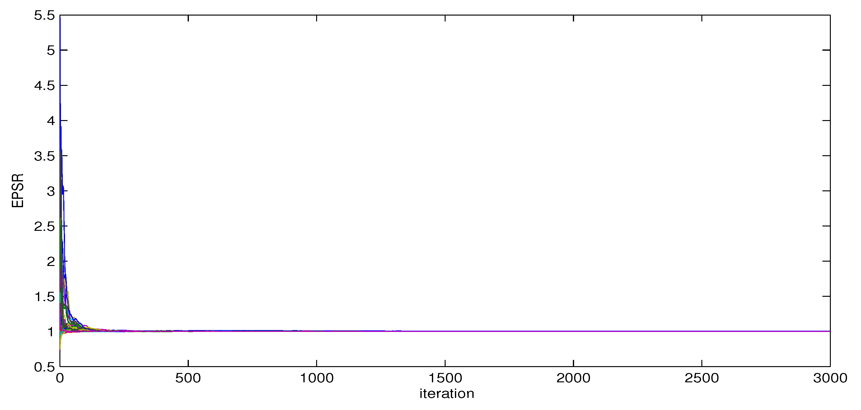
The MCMC algorithm described in Section 3 is implemented to obtain the estimates of unknown parameters θ . Before formal implementation, a few test runs were conducted as pilots to monitor the convergence of the Gibbs sampler. We plot the values of EPSR of unknown parameters against the number of iterations under three different starting values. For SS, Figure 2 presents the plots of EPSR of unknown parameters under three different starting value with sample size n = 400 .
It can be found that the convergence of estimates is fast and all values of EPSR are less than 1.2 in about 300 iterations. To be conservative, we remove the first 2000 observations as burn-in phrase and further collect 3000 observations for calculating the bias (BIAS), the root mean squares (RMS) and the standard deviation (SD) of the estimate across 100 replications. The BIAS and RMS of the j-th component θ ^ j in estimates are defined as follows:
B I A S ( θ ^ j ) = ( θ ¯ j θ j 0 ) , θ ¯ j = 1 100 κ = 1 100 θ ^ j ( κ ) , R M S ( θ ^ j ) = 1 100 κ = 1 100 ( θ ^ j ( κ ) θ j 0 ) 2 ,
where θ j 0 is the j-th element of population parameters θ 0 . The summaries of estimates of main parameters under two scenarios are reported in Table 1 and Table 2, where the sums of SD and RMS across the estimates are presented in the last rows.
Examinations of Table 1 and Table 2 present the following findings: (i) Both methods produce satisfactory results and the performance of SS are slightly superior to that of BaLsso. For n = 400 , the total RMS and SD are 1.870 and 1.975 respectively under SS, and amount to 2.016 and 2.035 respectively under BaLsso; (ii) As expected, increasing the sample size improves the accuracy of the estimates both for SS and BaLsso.
Another simulation is conducted to assess the performance of the proposed method in the variable selection when the covariates and latent variables are correlated. In this setting, we generate covariates and latent factors jointly from the multivariate normal distribution with mean zeros and covariance matrix Σ ( 7 × 7 ) with Σ j k = ρ | j k | , where Σ j k is the ( j , k ) t h entry of Σ . We consider three scenarios for ρ : (i) ρ = 0.1 , (ii) ρ = 0.5 and (iii) ρ = 0.8 , which represents respectively the weak, the mild and the strong dependence among them. The values of β and ψ are taken as ( 1.0 , 0.0 , 1.0 , 0.0 , 1.0 , 0.0 , 1.0 ) and ( 1.0 , 0.0 , 1.0 , 0.0 , 1.0 , 1.0 , 0.0 ) respectively, and the sample size is taken as n = 1000 . The other model setups are set as the same as before. We implement MCMC sampling and collect 3000 observations after removing first 2000 observations for posterior inference. We follow [48] and treat a regression coefficient to be zero if the absolute value of its estimate is less than 0.1. Table 3 gives the summary of variable selection across 100 replications.
Based on Table 3, it can be found that (i) for nonzero regression coefficients, two methods exhibit satisfactory performances, both with 100% correct rates across all situations; (ii) for zero regression coefficients, there exist difference between two methods, and SS are uniformly outperforms BaLsso. The underlying reason perhaps is that for SS, the variances of estimates are set to be small enough to ensure the coefficients close to zero while for BaLsso, the variance of estimates are controlled by the shrinkage parameters which may not be large enough to ensure this point; (iii) with the increase of the strength of dependence, the correct rates of two methods decreases.

5. China Household Finance Survey Data

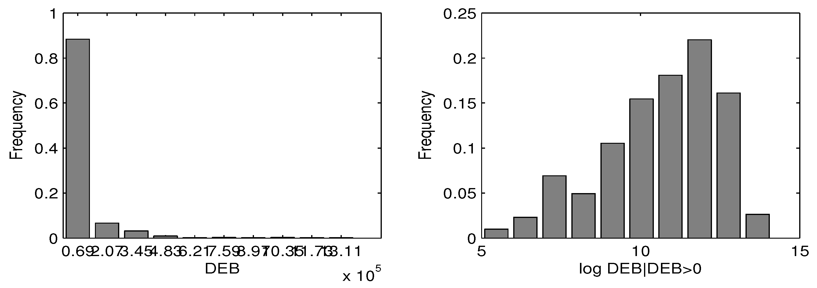
To demonstrate the usefulness of the proposed methodology, in this section a small portion of Chinese household finance debt data is analyzed. The dataset is collected from the China household financial survey (CHFS), a non-profit institute organized by the Southeast University of Finance and Economics. The survey covers a series of questions which touch on the information about various aspects of the household’s financial situation. In this study, we only focus on the measurement `gross debts per household (DEB)’, the amount of the secured debt and unsecured debt of a household under investigation. We extracted them from the survey of Zhejiang Province in 2013. Due to some uncertain factors, some measurements in DEB are missing. The missing proportion is about 2.7%. We remove the subjects with missing entries and the ultimate sample size is 884. A preliminary data analysis shows that the measurements DEB contain excessive zeros and the proportion of zeros is about 72.58%. Naturally, we treat this variable as the outcome variable s i , and identify it with u i and z i . Figure 3 presents the histogram of DEB as well as the logarithms of positive values. It can be seen clearly that dataset illustrates strong heterogeneity. The skewness and kurtosis of DEB are 1.1042 and 2.3361, respectively, which indicates that single parametric model for DEB may be unappreciated.
We include the following measurements as the potential explanatory factors to interpret the variability in DEB: gender ( x 1 ), age ( x 2 ) , marital status ( x 3 ), health condition( x 4 ), educational experience ( x 5 ), employment status of the household head ( x 6 ), the number of family members (aged over 16, x 7 ), and the household annual income ( x 8 ). Table 4 gives the descriptive summary of the measurements under consideration. To unify the scale, all covariates were standardized.
Besides the observed factors mentioned above, we also include family culture η , a latent factor into current analysis. It is well-known that China is an ancient civilization country with a long history, and Confucian culture has deeply rooted in the social development. Economic activity or social development can not be independent of cultural development. Hence, it is of practical interest to investigate how the family culture affect the behaviour of the household finance debt. Based on the design of the questionnaire, we select the following three measurements as manifestations for η :(i) boys’s preference (BP, y 1 ). This is a three-category measurement coded by 0, 1 and 2, which corresponds to the attitude `oppositive’, `does’t matter’ and `strongly support’; (ii) attitude toward to the single of children (SC), coded by 0, 1 and 2, according to the leve of support; (iii) importance of a household head in a family.This measurement is originally coded in point 0 to 5 according to the support level. However, in view of that the frequencies in the last three groups are small, we group them into three categories and recode them by 0 (does not matter), 1(important) and 2 (very important). In addition, due to that some manifestations are missing, we treat missing data as missing random and ignorable [49], and ignore the specific missing mechanic that results in missing data.
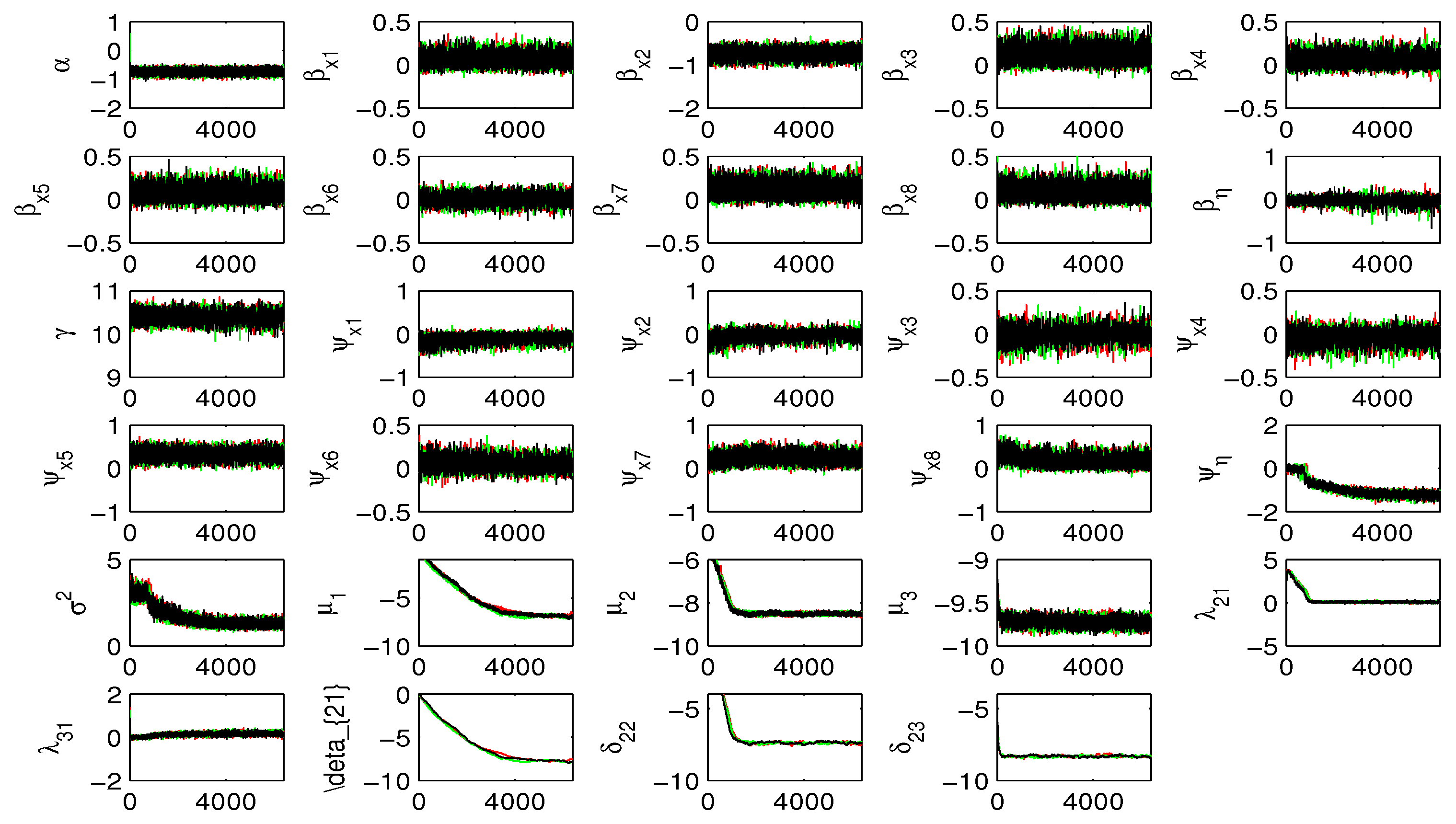
Let U = { u i } , Z = { z i } , and Y = { Y o b s , Y m i s } , where Y o b s is the collectionn of observed data and Y m i s is the set of missing data. We formulate U , Z and Y within equations (1), (2) and (5), and assume that η i , i i d . N ( 0 , 1 ) . The inputs of hyperparameters in the priors are taken as follows: Λ j 0 = 0.0 , H j 0 = 1 and η j 1 = η j 2 = η j 3 = 2.0 . The values of other hyperparameters are taken as the same as those in the simulation study. To implement MCMC sampling algorithm, we need to impute the missing data in Y . This is just to do by drawing y i j , m i s from the conditional distribution p ( y i j , m i s | θ , Y o b s ) = N ( μ j , m i s + Λ j , m i s η i , 1 ) , where μ j , m i s and Λ j , m i s are the components of μ and Λ respectively which corresponds to the missing entry y i j , m i s in y i . In addition, to identify the model and scale the factor, we set Λ 1 = 1 . We also adopt the method in [50] in the context of latent variable model with polytomous data and fix δ j 1 at Φ 1 ( f j 1 / n j ) , where n j is the size of y o b s , i j equal to 1, and f j 1 is the observed frequency of 0 in y o b s , i j . To assess the convergence of the algorithm, for SS, we plot the traces of estimates under three different initial values (see Figure 4). It can be seen that the algorithm converges at about 3000 iterations. To be conservative, we collect 6000 observations after deleting the initial 4000 observations for calculating the estimates and the standard deviations.
Table 6 gives the summary of the estimates of unknown parameters in two parts and factor loadings. Examinations of Table 6 show that most estimates are very close but there exists differences in the estimates of β 4 , β 5 , β 7 , β 8 , ψ 2 , ψ 7 and ψ 8 . For example, the estimates of β 4 , β 5 and β 7 under SS are 0.428 , 0.577 , 0.747 with standard deviations 0.062 , 0.070 and 0.072 respectively, while equal to 0.072 , 0.082 and 0.092 with standard deviations 0.07 , 0.081 and 0.092 under BaLsso. These differences reflect the fact that two methods impose different penalties on the regression coefficients in the variable selection.
Table 5. Estimates and standard deviations estimates of unknown parameters under SS and BaLsso: CHFS data.
SS BaLsso SS BaLsso
Par Est. SD Est. SD Par Est. SD Est. SD
α -0.835 0.078 -0.838 0.080 γ 9.782 0.152 9.670 0.125
β 1 0.050 0.063 0.076 0.070 ψ 1 -0.137 0.103 -0.107 0.088
β 2 -0.750 0.099 -0.757 0.102 ψ 2 -0.147 0.141 -0.015 0.081
β 3 0.107 0.085 0.147 0.088 ψ 3 -0.022 0.065 -0.006 0.075
β 4 0.428 0.062 0.072 0.070 ψ 4 -0.019 0.060 -0.029 0.069
β 5 0.577 0.070 0.082 0.081 ψ 5 0.259 0.123 0.322 0.107
β 6 0.004 0.040 0.005 0.052 ψ 6 0.035 0.058 0.053 0.067
β 7 0.118 0.079 0.130 0.079 ψ 7 0.043 0.072 0.281 0.113
β 8 0.747 0.073 0.092 0.077 ψ 8 0.384 0.132 0.188 0.118
β η -0.059 0.112 -0.039 0.092 ψ η 1.205 0.106 1.910 0.104
σ 2 0.312 0.150 0.300 0.152
λ 21 -0.791 0.062 -0.714 0.057
λ 31 -0.865 0.067 -0.625 0.068
To see more clearly, Table 4 gives the resulting selected variables according to SS and BaLsso. It can be seen that (i) for part one, both methods give the same results for the selection of factors `gender’, `age’, `material status’, `employment’, `number of adults’ and `family culture’. Two methods favor that `age’,`material status’, and `number of adults’ can be helpful in improving model fits while `gender’ and `family culture’ have less impacts on the probabilities of being held finance debt. However, there exist contradictory conclusion in selecting `health condition’, `education’ and `income’; (ii) for part two, except the factors `age’ and `number of adults’, two methods give the same results. In particular, both methods support that `family culture’ is relevant to the amount of household finance debts being held. This fact is also revealed by [17] in the analysis of CHFS by using two-part nonlinear latent variable model. The further interpretation is omitted for saving spaces.

6. Discussion

Two-part latent variable model can be considered as an extension of traditional two-part model to the situations where the latent variables are included to identify the unobserved heterogeneity of population resulting from the absence of the observed covariates. When analyzing such a model, an important issue is to determine which factor is relevant to the outcome variable. This is especially true when the number of exogenous factors is high because the usual model selection/comparison procedure is extremely time-consuming. In this paper, we restor to the Bayesian variable selection method and developed a fully Bayesian variable selection procedure for the semi-continuous data. Our formulation is along the lines with the spike and slab bimodal prior and recast the distribution of regression coefficients and factor loadings as hierarchy of priors over the parameter and model space. The selected variables is identified with high posterior probability of occurrence. We also consider a adaptive Bayesian lasso (BaLsso) for reference. To facilitate the computation, we recast the logistic regression model in part one as the flavor of normal mixture model by introducing latent Polya-gamma variables. which admits the conjugate conjugate full-conditional distributions for all regression coefficients, factor loadings and factor variables.
Although the Bayesian variable selection has its unique advantage, there are still some limitations that need to be considered with care. First, its computational complexity is high. Bayes SSL requires Monte Carlo sampling to estimate the posterior distribution, which can lead to slower calculation speed, especially when working with high-dimensional data sets. Secondly, the method is sensitive to hyperparameter and data distribution assumptions. The selection of the hyperparameters of the prior distribution, such as the ratio of spike to slab, lasso penalty parameters, and data distribution assumptions, will have a great impact on the results. When the data does not conform to the model convention, the performance of the model is poor. Therefore, these issues need to be carefully considered in practical application to ensure that the Bayesian SS method can be effectively applied to specific data sets.
The existing applications of the proposed methodology can be applied to more general latent variable models that include the the multilevel SEMs [50] and longitudinal dynamic variable models [16,51] with discrete variables. These extensions are left for further study.

Funding

This research was funded by National Nature Science Foundation of China (NNSF 11471161) and Natural Science Foundation of the Higher Education Institutions of Jiangsu Province (15KJB110010).

Acknowledgments

We are thankful to Professor Xin-Yuan Song, Department of Statistics, The Chinsese University of Hong Kong, Hong Kong, for providing us CHFS data.

Conflicts of Interest

The authors declare no conflict of interest.

Abbreviations

The following abbreviations are used in this manuscript:
TPM Two-part model
TPLVM Two-part latent variable model
SS Spike and slab bimodal prior
BaLsso Bayesian lasso
MCMC Markov Chains Monte Carlo
CHFS China household finance survey

Appendix A

In this section, we will present some technical details on the full conditionals in the MCMC sampling. For ease of exposition, for any scalar or vector x, we use p ( x | ) to denote the conditional distribution of x given `⋯’. Note that under the scenarios SS and BaLsso, the full conditionals of Ω , U * , Y * and θ are exactly the same. The following derivations are mainly based on the Bayes theorem.
1. Full conditional of p ( Ω | )
It follows from (8), (2) and (5) that
p ( Ω | ) = i = 1 n p ( ω i | ) ,
where
p ( ω i | ) p ( u i , u i * | ω i , α , β ) p ( z i | u i , ω i , γ , ψ , σ 2 ) p ( y i * | ω i , μ , Λ ) p ( ω i | Φ ) .
Let κ i * = κ i u i * ( γ + x i T β x ) , z i * = z i γ x i T ψ x . By some algebra, it can be shown that
p ( ω i | ) = D N m ( μ ^ ω i , Σ ^ ω i ) ,
where
μ ^ ω i = Σ ^ ω i β ω κ i * + ψ ω u i z i * / σ 2 + Λ T ( y i * μ ) , Σ ^ ω i = β ω β ω T u i * + ψ ω ψ ω T u i / σ 2 + Λ T Λ + Φ 1 1 .
Hence, draw of Ω can be obtained by simulating ω i independently from the normal distribution (A1).
2. Full conditional of p ( U * | )
Following the similar derivation in [41], it can be shown that given U , Ω and θ , U * is the entilted Polya-Gamma distribution given by
p ( U * ) = i = 1 n P G ( u i * | 1 , η i )
where η i = α + β T w i . Drawing u i from this distribution can be achieved via rejection sampling, see [41] or [52] for more details on this issue.
3. Full of conditional of p ( Y * | )
Note that
p ( Y * | ) p ( Y | Y * , δ ) p ( Y * | Ω , μ , Λ ) = i = 1 n k = 1 p = 0 c I { y i k = , δ k < y i k * δ k + 1 } × 1 2 π exp 1 2 ( y i k * μ k Λ k T ω i ) 2 .
Hence, given Ω , the full conditional of Y * only depends on μ , Λ , Y and Ω , and is given by
p ( Y * | ) = i = 1 n k = 1 p p ( y i k * | ω i , θ , y i k ) , p ( y i k * | ω i , θ , y i k ) = N ( μ k + Λ k T ω i , 1 ) I { δ k , y i k < y i k * δ k , y i k + 1 } .
This is the truncated normal distribution and its draw can be obtained via inverse distribution sampling method, see for example, [53].
4. Full conditional of p ( θ | )
Recall that θ is consisted of α , β , γ , ψ , σ 2 , μ , Λ , Φ and δ . Hence, draw of θ can be accomplished by (i) drawing α from p ( α | ) , (ii) drawing β from p ( β | ) , (iii) drawing γ from p ( γ | ) , (iv) drawing ( ψ , σ 2 ) from p ( ψ , σ 2 | ) , (v) drawing μ from p ( μ | ) , (vi) drawing Λ from p ( α | ) , (vii) drawing Φ form p ( Φ | ) , and (viii) drawing δ from p ( δ | ) sequentially. Note that given U * , Y * and Ω , the models (8), (2) and (5) reduce to the ordinary regression models, and hence most of full conditionals, similar to that of the regression coefficients and variance/covariance in the Bayesian regression analysis, are the standard distributions such as normal, gamma, inverse gamma and wishart distributions. As a matter of fact, by some tedious but non-trivial calculations, it can be shown that
p ( α | ) = N ( μ ^ β , σ ^ β 2 ) , p ( β | ) = N q ( μ ^ β , Σ ^ β ) ,
p ( γ | ) = N ( μ ^ γ , σ ^ γ 2 ) , p ( ψ , σ 2 | ) = I G ( α ^ σ , β ^ σ ) × N q ( μ ^ ψ , σ 2 Σ ^ ψ ) ,
p ( μ | Ω , Λ , Y * ) = N p ( m ^ μ , Σ ^ μ ) , p ( Λ | ) = k = 1 p p ( Λ k | ) = k = 1 p N m ( Λ ^ k , H ^ k ) ,
p ( Φ 1 | ) = W m ( ρ + n , R ^ ) ,
in which
μ ^ α = σ ^ α 2 i = 1 n ( κ i u i * β T w i ) , σ ^ α 2 = ( i = 1 n u i * + σ α 0 2 ) 1 , μ ^ β = Σ ^ β i = 1 n w i ( κ i α u i * ) , Σ ^ β 1 = i = 1 n u i * w i w i + d i a g { γ β 2 } , μ ^ γ = σ ^ γ 2 i = 1 n u i ( z i ψ T w i ) / σ 2 , σ ^ γ 2 = ( i = 1 n u i / σ 2 + σ γ 0 2 ) 1 , μ ^ ψ = Σ ^ ψ i = 1 n w i ( z i γ ) u i / σ 2 , Σ ^ ψ 1 = i = 1 n u i w i w i + d i a g { γ ψ 2 } , α ^ σ = a 0 + | I | / 2 , β ^ σ = b 0 + 1 2 ( i = 1 n u i z i 2 μ ^ ψ T Σ ^ ψ 1 μ ^ ψ + Λ 0 k T H 0 k 1 Λ 0 k ) , m ^ μ = Σ ^ μ ( Σ 0 1 μ 0 + n ( Y ¯ * Λ Ω ¯ ) ) , Σ ^ μ 1 = n I p + Σ 0 1 , Λ ^ k = H ^ k ( H 0 k 1 Λ 0 k + Ω T Y [ k ] * * ) , H ^ k 1 = n Φ 1 + Ω T Ω , R ^ 1 = R 0 1 + Ω T Ω ,
where Y * * is the n × p matrix with the i t h row y i * T μ T , Y [ k ] * * is the k t h column of Y * * , and Ω is the n × m matrix with the i t h row ω i ; Y ¯ * = i = 1 n y i * / n , Ω ¯ = i = 1 n ω i / n . are the sample means of Y * and Ω and | I | denotes the size of I = { u i = 1 } .
However, for δ , we note that
p ( δ | ) = k = 1 p p ( δ k | Y [ k ] * , Y [ k ] ) , and p ( δ k | Y [ k ] * , Y [ k ] ) p ( δ k ) i = 1 n = 0 c I { y i k = , δ k < y i k * δ k , + 1 } .
Hence, drawing δ can be obtained by drawing δ k from p ( δ k | ) independently. Moreover, under prior (24), it can be shown that
p ( δ k | δ k , ( ) , Y [ k ] * , Y [ k ] ) p ( δ k , δ k , ( ) ) I { max y i k = 1 { y i k * } , δ k < min y i k = { y i k * } } .
where δ k , ( ) is the vector of δ k with δ k removed. Let h k , = max { δ k , 1 , max y i k = 1 { y i k * } } , g k , = min { δ k , + 1 , min y i k = { y i k * } } . It follows from (25) that
F 0 ( δ k ) F 0 ( δ k , 1 ) F 0 ( δ k , + 1 ) F 0 ( δ k , 1 ) | δ k , , Y [ k ] * , Y [ k ] B e t a ( η k , , η k , + 1 ) I { ( s k , , t k , ) } ,
where
s k , = F 0 ( h k , ) F 0 ( δ k , 1 ) F 0 ( δ k , + 1 ) F 0 ( δ k , 1 ) , t k , = F 0 ( g k , ) F 0 ( δ k , 1 ) F 0 ( δ k , + 1 ) F 0 ( δ k , 1 ) .
As a result, we can draw δ k by first generating a δ k * from the truncated beta distribution (A8) and then transform it to the δ k l via inverse-transformation by setting F 0 1 ( δ k * [ F 0 ( δ k , + 1 ) F 0 ( δ k , 1 ) ] + F 0 ( δ k , 1 ) ) . A draw of truncated beta distribution can be obtained by implementing inverse-distribution sampling method.
4. Full conditional of p ( Q * | )
First of all, it is noted that Q * is consisted of F β , F ψ , w β , w ψ , η β 2 , and η ψ 2 under SS, and formed by γ β 2 , γ ψ 2 , λ β 2 and λ ψ 2 under BaLsso. Similar to that of θ , we update Q * by drawing observations from their full conditionals per component sequentially.
Firstly, it is noted that
p ( F β | ) k = 1 q p ( β k | f β k , η β k 2 ) p ( f β k | w β ) , p ( F ψ | ) k = 1 q p ( ψ k | σ 2 , f ψ k , η ψ k 2 ) p ( f ψ k | w ψ ) ,
which indicates that the components in the posteriors of F β and F ψ are independent. Further, it follows easily from (12) that
p ( f β k | w β , η β k 2 , β k ) = ( 1 q ^ β k ) δ ν β 0 ( · ) + q ^ β k δ 1 ( · ) , p ( f ψ k | w ψ , η ψ k 2 , β k ) = ( 1 q ^ ψ k ) δ ν ψ 0 ( · ) + q ^ ψ k δ 1 ( · ) ,
where
q ^ β k = w β ϕ ( β k / η β k ) ( 1 w β ) ϕ ( β k / ( ν β 0 η β k ) / ν β 0 + w β ϕ ( β k / η β k ) , q ^ ψ k = w ψ ϕ ( ψ k / ( σ η ψ k ) ( 1 w ψ ) ϕ ( ψ k / ( σ ν ψ 0 η ψ k ) / ν ψ 0 + w ψ ϕ ( ψ k / ( σ η ψ k ) ) ,
and ϕ ( · ) is the standard normal probability density function.
Secondly, it is noted that
p ( w β | F β ) p ( w β ) p ( F β | w β ) = p ( w β ) k = 1 q p ( f β k | w β ) = c w β a β 1 ( 1 w β ) b β 1 k = 1 q w p I { f β k = 1 } ( 1 w β ) I { f β k = ν β 0 } , p ( w ψ | F ψ ) p ( w ψ ) p ( F ψ | w ψ ) = p ( w ψ ) k = 1 q p ( f ψ k | w ψ ) = c w p a ψ 1 ( 1 w β ) b ψ 1 k = 1 q w ψ I { f ψ k = 1 } ( 1 w ψ ) I { f ψ k = ν ψ 0 } .
Hence,
p ( w β | ) = B e t a ( c β 1 + | { f β k = 1 } | , c β 2 + | { f β k = ν β 0 } | ) ,
p ( w ψ | ) = B e t a ( c ψ 1 + | { f ψ k = 1 } | , c ψ 2 + | { f ψ k = ν ψ 0 } | ) ,
where | A | , as before, is the size of set A.
Lastly, it follows from
p ( η β 2 | F β , β ) p ( β | F β , η β 2 ) p ( η β 2 ) = k = 1 q ( η β k 2 ) 1 / 2 exp 1 2 η β k 2 β k 2 / f β k ( η β k 2 ) a β 1 1 exp { a β 2 η β k 2 } , p ( η ψ 2 | F ψ , ψ ) p ( ψ | F ψ , η ψ 2 ) p ( η ψ 2 ) = k = 1 q ( η ψ k 2 ) 1 / 2 exp 1 2 η ψ k 2 ψ k 2 / f ψ k ( η ψ k 2 ) a ψ 1 1 exp { a β 2 η ψ k 2 }
that
p ( η β 2 | F β , β ) = k = 1 q p ( η β k 2 | f β k , β k ) = k = 1 q G a ( τ ^ β k , ζ ^ β k ) , p ( η ψ 2 | F ψ , ψ ) = k = 1 q p ( η ψ k 2 | f ψ k , ψ k ) k = 1 q G a ( τ ^ ψ k , ζ ^ ψ k ) ,
where
τ ^ β k = τ β 0 + 1 / 2 , ζ ^ β k = ζ β 0 + β k 2 / ( 2 f β k ) , τ ^ ψ k = τ ψ 0 + 1 / 2 , ζ ^ ψ k = ζ ψ 2 + ψ k 2 / ( 2 f ψ k ) .
For BaLasso, we follow the practice in [37]) and can show
p ( γ β 2 | ) = k = 1 q p ( γ β k 2 | ) = k = 1 q I G ( μ ^ β , λ ^ β ) , p ( γ ψ 2 | ) = k = 1 q p ( γ ψ k 2 | ) = k = 1 q I G ( μ ^ ψ , λ ^ ψ ) ,
in which
μ ^ β = λ ^ β / β j 2 , λ ^ β = λ β k 2 , μ ^ ψ = σ 2 λ ^ ψ / β j 2 , λ ^ ψ = λ ψ k 2 ,
where I G ( μ , λ ) is the inverse-gaussian distribution with density λ / ( 2 π ) x 3 / 2 exp { λ ( x μ ) 2 / ( 2 μ 2 x ) } ( x > 0 ) [54].
Similarly,
p ( λ β 2 | ) = k = 1 q p ( λ β k 2 | ) = k = 1 q G a ( a ^ β k , b ^ β k ) , p ( λ ψ 2 | ) = k = 1 q p ( λ ψ k 2 | ) = k = 1 q G a ( c ^ ψ k , d ^ ψ k ) ,
in which
a ^ β k = a k 0 + 1.0 , b ^ β k = b k 0 + 0.5 γ β k 2 , c ^ ψ k = c k 0 + 1.0 , d ^ ψ k = d k 0 + 0.5 γ ψ k 2 .

References

  1. Deb, P.; Munkin, M.K.; Trivedic, R.K. Bayesian analysis of the two-part model with endogeneity: Application to health care expenditure. J. Appl. Econ. 2006, 21, 1081–1099. [Google Scholar] [CrossRef]
  2. Cragg, J.G. Some statistical models for limited dependent variables with application to the demand for durable goods. Econometrica 2006, 39, 829–844. [Google Scholar] [CrossRef]
  3. Neelon, B.; Zhu, L.; Neelon, S.E.B. Bayesian two-part spatial models for semicontinuous data with application to emergency department expenditures. Biostatistics 2015, 16, 465–479. [Google Scholar] [CrossRef]
  4. Manning, W.G.; et al. (1981). A two-part model of the demand for medical Care: preliminary results from the health insurance experiment, in Health, Economics, and Health Economics, eds. van der Gaag, J. and Perlman, M., p. 103-104, Amsterdam: North-Holland.
  5. Su, L.; Tom, B.D.; Farewell, V.T. Bias in 2-part mixed models for longitudinal semi-continuous data. Biostatistics 2009, 10, 374–389. [Google Scholar] [CrossRef]
  6. Su, L.; Tom, B.D.; Farewell, V.T. A likelihood-based two-part marginal model for longitudinal semi-continuous data. Statiscal Methods in Medical Research 2015, 24, 194–205. [Google Scholar] [CrossRef]
  7. Liu, L.; Cowen, M.E.; Strawderman, R.L.; Shih, Y.C.T. A flexible two-part random effects model for correlated medical costs. Journal of Health Economics 2010, 29, 110–123. [Google Scholar] [CrossRef]
  8. Smith, V.A.; Neelon, B.; Preisser, J.S.; Maciejewski, L. A marginalized two-part model for semicontinuous data. Statistics in Medicine 2015, 33, 4891–4903. [Google Scholar] [CrossRef] [PubMed]
  9. Tooze, J.A.; Grunwald, J.K.; Jones, R.H. Analysis of repeated measures data with clumping at zero. Statistical Methods in Medical Research 2002, 11, 341–355. [Google Scholar] [CrossRef]
  10. Brown, R.A.; Monti, P.M.; Myers, M.G.; Martin, R.A.; Rivinus, T.; Dubreuil, M.E.T.; Rohsenow, D.J. Depression among cocaine abusers in treatment: Relation to cocaine and alcohol use and treatment outcome. American Journal of Psychiatry 1998, 155, 220–225. [Google Scholar] [CrossRef]
  11. Olsen, M.K.; Schafer, J.L. A two-part random-effects model for semicontinuous longitudinal data. Journal of the American Statistical Association 2001, 96, 730–745. [Google Scholar] [CrossRef]
  12. Xing, D.Y.; Huang, Y.X.; Chen, H.N.; Zhu, Y.L.; Dagen, G.A.; Baldwin, J. Bayesian inference for two-part mixed effects model using skew distributions, with application to longitudinal semi-continuous alcohol data. Statistical Methods in Medical Research 2017, 26, 1838–1853. [Google Scholar] [CrossRef]
  13. Chen, J.Y.; Zheng, L.Y.; Xia, Y.M. Bayesian analysis for two-part latent variable model with application to fractional data. Communications in Statistics - Theory and Methods 2023. [Google Scholar] [CrossRef]
  14. Kim, Y.; Muthén, B.O. Two-Part Factor Mixture Modeling: Application to an Aggressive Behavior Measurement Instrument. Structural Equation Modeling: A Multidisciplinary Journal 2009, 16, 602–624. [Google Scholar] [CrossRef]
  15. Feng, X.; Lu, B.; Song, X.; Ma, S. Financial literacy and household finances: A Bayesian two-part latent variable modeling approach. Journal of Empirical Finance 2019, 51, 119–137. [Google Scholar] [CrossRef]
  16. Xia, Y.M.; Tang, N.S. Bayesian analysis for mixture of latent variable hidden Markov models with multivariate longitudinal data. Computational Statistics & Data Analysis 2019, 132, 190–211. [Google Scholar]
  17. Gou, J.W.; Xia, Y.M.; Jiang, D.P. Bayesian analysis of two-part nonlinear latent variable model: Semiparametric method. Statistical Moddelling 2023, 23, 721–741. [Google Scholar] [CrossRef]
  18. Xiong, S.C.; Xia, Y.M.; Lu, B. Bayesian Analysis of Two-Part Latent Variable Model with Mixed Data. Communications in Mathematics and Statistics in press. 2023. [Google Scholar] [CrossRef]
  19. Fan, J.; Li, R. Variable selection via nonconcave penalized likelihood and its oracle properties. Journal of the American Statistical Association 2001, 96, 1348–1360. [Google Scholar] [CrossRef]
  20. Fu, W.J. Penalized regression: the bridge versus the lasso. Journal of computational and Graphical Statistics 1998, 7, 109–148. [Google Scholar] [CrossRef]
  21. Hastie, T.; Tibshirani, R.; Friedman, J. The Elements ofStatistical Learning; Springer-Verlag: New York, NY, 2009. [Google Scholar]
  22. Hastie, T. , Tibshirani, R. and Wainwright, M. (2015). Statistical Learning with Sparsity - The Lasso and Generalization, CRC Press: New York.
  23. Kuo, L.; Mallick, B.K. Variable selection for regression models. Sankhya, Ser. B 1998, 60, 65–81. [Google Scholar]
  24. Tibshirani, R. Regression shrinkage and selection via theLasso. J. R. Stat. Soc. B 1996, 58, 267–288. [Google Scholar] [CrossRef]
  25. Zou, H.; Hastie, T. Regularization and variable selectionvia the elastic net. Zou, H., and Hastie, T. 2005, 67, 301–320. [Google Scholar]
  26. Zou, H. The adaptive Lasso and its oracle properties. Journal of the American statistical Association 2006, 101, 1418–1429. [Google Scholar] [CrossRef]
  27. Zhang, W.; Ota, T.; Shridhar, V.; Chien, J.; Wu, B.; et al. Networkbased survival analysis reveals subnetwork signatures for predicting outcomes of ovarian cancer treatment. PLOS Comput. Biol. 2013, 9, e1002975. [Google Scholar] [CrossRef] [PubMed]
  28. Zhao, Q.; Shi, X.; Xie, Y.; Huang, J.; Shia, B.; et al. Combiningmultidimensional genomic measurements for predicting cancerprognosis: observations from TCGA.Brief. Bioinform 2014, 16, 291–303. [Google Scholar]
  29. George, E.I.; McCulloch, R.E. Variable selection via Gibbs sampling. Journal of the American Statistical Association 1993, 88, 881–889. [Google Scholar] [CrossRef]
  30. George, E.I.; McCulloch, R.E. Approaches for Bayesianvariable selection. Stat. Sin. 1997, 7, 339–373. [Google Scholar]
  31. Chipman, H.A. Bayesian variable selection with related predictors. Canad. J. Statist. 1996, 24, 17–36. [Google Scholar] [CrossRef]
  32. Ishwaran, H.; Rao, J.S. Spike and Slab gene selcetion for multigroup microarray data. Journal of the American Statistical Association 2005, 87, 371–390. [Google Scholar]
  33. Ishwaran, H.; Rao, J.S. Spike and Slab variable selection: frequentist and Bayesian strageies. The Annals of Statistics 2005, 33, 730–773. [Google Scholar] [CrossRef]
  34. Mitchell, T.J.; Beauchamp, J.J. Bayesian variable selection in linear regression. Journal of the American Statistical Association 1988, 83, 1023–1032. [Google Scholar] [CrossRef]
  35. Rockova, V.; George, E.I. EMVS: The EM approach toBayesian variable selection. Journal of the American Statistical Association 2014, 109, 828–846. [Google Scholar] [CrossRef]
  36. Tang, Z.X.; Shen, Y.P.; Xinyan Zhang, X.Y.; Nengjun Yi, N.J. The Spike-and-Slab Lasso Generalized Linear Modelsfor Prediction and Associated Genes Detection. Genetics 2017, 205, 77–88. [Google Scholar] [CrossRef]
  37. Park, T.; Casella, G. The Bayesian Lasso, Journal of the American Statistical Association 2008, 482, 681–686. [Google Scholar] [CrossRef]
  38. Skrondal, A.; Rabe-Hesketh, S. Generalized latent variable modelling: multilevel, longitudinal and structural equation models; Chapman & Hall/CRC: London.
  39. Bollen, K.A. Structural Equations with Latent Variables; John Wiley & Sons: New York, 1989. [Google Scholar]
  40. Lee, S. Y. (2007). Structural Equation Modeling: A Bayesian Approach, John Wiley & Sons: New York.
  41. Polson, N.G.; Scott, J.G.; Windle, J. Bayesian Inference for Logistic Models Using Polya-Gamma Latent Variables. Journal of the American Statistical Association 2013, 108, 1339–1349. [Google Scholar] [CrossRef]
  42. Anderson, T. W. (1984). An Introduction to Multivariate Statistical Analysis, John Wiley & Sons: New York.
  43. Sha, N.J.; Dechi, B.O. A Bayes inference for ordinal response with latent variable approach. Stats 2019, 2, 321–331. [Google Scholar] [CrossRef]
  44. Tanner, M.A.; Wong, W.H. The calculation of posterior distributions by data augmentation(with discussion). Journal of the American statistical Association 1987, 82, 528–550. [Google Scholar] [CrossRef]
  45. Gelfand, A.E.; Smith, A.F.M. Sampling-based approaches to calculating marginal densities. Journal of the American Statistical Association 1990, 85, 398–409. [Google Scholar] [CrossRef]
  46. Geman, S.; Geman, D. Stochastic relaxation, Gibbs distribution, and the Bayesian restoration of images. IEEE Transactions on Pattern Analysis and Machine Intelligence 1984, PAMI-6, 721–741. [Google Scholar] [CrossRef]
  47. Gelman, A.; Rubin, D.B. Inference from iterative simulation using multiple sequences (with discussion). Statistical Science 1992, 7, 457–511. [Google Scholar] [CrossRef]
  48. Feng, X.; Wang, Y.F.; Lu, B.; Song, X.Y. Bayesian regularized quantile structural equation models. Journal of Multivariate Analysis 2017, 154, 234–248. [Google Scholar] [CrossRef]
  49. Little, R.J.A.; Rubin, D.B. Statistical analysis with missing data, second Edition ed; John Wiley & Sons: New York, 2002. [Google Scholar]
  50. Song, X.Y.; Lee, S.Y. A tutorial on the Bayesian approach for analyzing structural equation models. Journal of Mathematical Psychology 2012, 56, 135–148. [Google Scholar] [CrossRef]
  51. Song, X.Y.; Xia, Y.M.; Zhu, H.T. Hidden Markov latent variable models with multivariate longitudinal data. Biometrics 2017, 73, 313–323. [Google Scholar] [CrossRef]
  52. Devroye, L. (1986). Non-Uniform Random Variate Generation, Springer-Verlag: New York.
  53. Ross, S. M. (1991). A Course in Simulation, MacMillan: New York.
  54. Chhikara, R. S. , and Folks, L. (1989). The Inverse Gaussian Distribution: Theory, Methodology, and Applications, Marcel Dekker: New York.
  55. Duan, N.; Manning, W.G.; Morris, C.N.; Newhouse, J.P. A Comparison of alternative models for the demand for medical Care. Journal of Business and Economic Statistics 1983, 1, 115–126. [Google Scholar] [CrossRef]
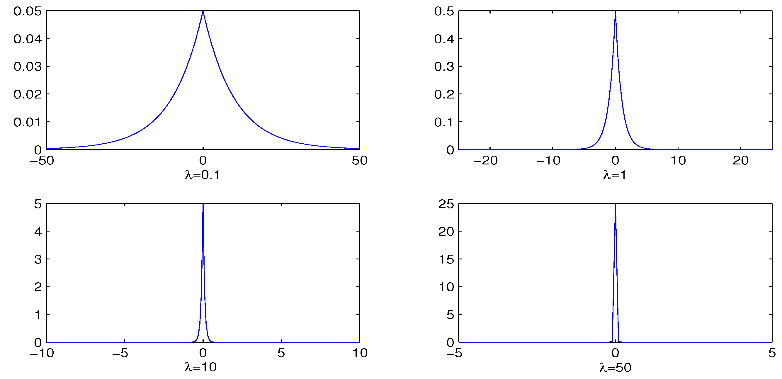
Figure 1. Plot of the densities of Laplace distribution across different choices of λ .
Preprints 97816 g001
Figure 2. Plot of the values of EPSR of unknown parameters under three different starting values: simulation study and n = 400 .
Preprints 97816 g002
Figure 3. Histograms of DEB and the logarithms of their positive values: China household finance survey data. Left panel corresponding the DEB and right panel corresponding to log ( DEB | DEB > 0 ) .
Preprints 97816 g003
Figure 4. Trace plots of the estimates of unknown parameters against the number of iteration under SS prior: CHFS data.
Preprints 97816 g004
Table 1. Summary of the estimates of unknown parameters under SS and BaLsso: simulation study and n = 400 .
SS BaLsso
PAR BIAS RMS SD BIAS RMS SD
α = 0.7 -0.015 0.097 0.129 0.028 0.150 0.134
β 1 = 0.7 -0.056 0.143 0.142 -0.152 0.217 0.136
β 2 = 0.0 -0.001 0.021 0.061 -0.019 0.042 0.079
β 3 = 0.7 -0.144 0.216 0.145 -0.122 0.251 0.148
β 4 = 0.0 0.005 0.030 0.064 -0.008 0.040 0.078
β 5 = 0.7 -0.091 0.147 0.137 -0.045 0.135 0.137
β 6 = 0.0 0.017 0.028 0.075 0.026 0.055 0.096
β 7 = 0.8 -0.187 0.237 0.184 -0.126 0.209 0.184
γ = 0.7 0.010 0.079 0.084 0.008 0.063 0.085
ψ 1 = 0.7 -0.035 0.079 0.077 -0.011 0.065 0.074
ψ 2 = 0.0 0.005 0.032 0.051 -0.018 0.031 0.054
ψ 3 = 0.7 -0.007 0.061 0.070 -0.021 0.085 0.069
ψ 4 = 0.0 -0.007 0.029 0.049 -0.003 0.031 0.053
ψ 5 = 0.7 -0.070 0.093 0.077 -0.018 0.082 0.075
ψ 6 = 0.8 -0.040 0.086 0.089 -0.02 0.069 0.088
ψ 7 = 0.0 -0.011 0.033 0.062 0.014 0.036 0.069
σ 2 = 1.0 0.085 0.129 0.117 0.038 0.082 0.111
λ 21 = 0.8 0.042 0.078 0.073 0.058 0.098 0.071
λ 31 = 0.8 0.030 0.072 0.071 0.034 0.063 0.072
λ 52 = 0.8 0.058 0.079 0.072 0.052 0.090 0.073
λ 62 = 0.8 0.031 0.060 0.072 0.037 0.064 0.073
Φ 12 = 0.3 0.014 0.041 0.074 0.018 0.058 0.076
Total - 1.870 1.975 - 2.016 2.035
Table 2. Summary of the estimates of unknown parameters under SS and BaLsso: simulation study and n = 1000 .
SS BaLsso
PAR BIAS RMS SD BIAS RMS SD
α = 0.7 0.052 0.096 0.087 0.009 0.092 0.087
β 1 = 0.7 0.005 0.069 0.089 0.055 0.117 0.090
β 2 = 0.0 0.003 0.048 0.058 0.032 0.052 0.060
β 3 = 0.7 0.007 0.086 0.093 -0.045 0.076 0.091
β 4 = 0.0 0.004 0.015 0.049 -0.020 0.043 0.060
β 5 = 0.7 0.010 0.071 0.086 0.013 0.074 0.085
β 6 = 0.0 -0.003 0.029 0.059 0.032 0.064 0.077
β 7 = 0.8 0.002 0.102 0.120 -0.042 0.108 0.114
γ = 0.7 0.017 0.042 0.053 0.030 0.056 0.054
ψ 1 = 0.7 -0.023 0.038 0.046 -0.016 0.039 0.047
ψ 2 = 0.0 -0.007 0.019 0.033 -0.005 0.018 0.037
ψ 3 = 0.7 -0.028 0.060 0.042 -0.014 0.026 0.043
ψ 4 = 0.0 -0.007 0.023 0.033 0.000 0.018 0.036
ψ 5 = 0.7 -0.005 0.035 0.046 0.003 0.043 0.047
ψ 6 = 0.8 -0.031 0.058 0.053 -0.039 0.063 0.054
ψ 7 = 0.0 -0.001 0.031 0.045 -0.025 0.081 0.053
σ 2 = 1.0 0.018 0.049 0.068 0.041 0.053 0.071
λ 21 = 0.8 0.021 0.041 0.045 0.033 0.038 0.045
λ 31 = 0.8 0.016 0.049 0.045 0.028 0.038 0.045
λ 52 = 0.8 0.032 0.049 0.045 0.054 0.057 0.045
λ 62 = 0.8 0.043 0.059 0.046 0.043 0.054 0.046
Φ 12 0.016 0.043 0.049 0.005 0.037 0.048
Total - 1.112 1.29 - 1.247 1.335
Table 3. Number of correctly selected variables in the two-part model on the simulated data sets.
SS BaLsso
PAR ρ = 0.1 ρ = 0.5 ρ = 0.8 ρ = 0.1 ρ = 0.5 ρ = 0.8
β 1 = 1.0 100 100 100 100 100 100
β 2 = 0.0 98 96 85 88 86 76
β 3 = 1.0 100 100 100 100 100 100
β 4 = 0.0 96 95 86 93 93 85
β 5 = 1.0 100 100 100 100 100 100
β 6 = 0.0 96 94 93 97 92 87
β 7 = 1.0 100 100 100 100 100 100
ψ 1 = 1.0 99 100 100 100 100 100
ψ 2 = 0.0 100 99 95 100 98 93
ψ 3 = 1.0 100 100 100 100 100 100
ψ 4 = 0.0 100 100 97 98 100 91
ψ 5 = 1.0 100 100 100 100 100 100
ψ 6 = 1.0 100 100 100 100 100 100
ψ 7 = 0.0 100 98 97 97 96 96
Table 4. Descriptive statistics of explanatory variables: CHFS data .
Variable. Description. Mean. Max. Min. SD
Gender ( x 1 ) =1, male; =0, otherwise 0.756 1 0 0.430
Age ( x 2 ) 51.81 91 19 14.931
Marital status ( x 3 ) =1, married; 0, otherwise 0.863 1 0 0.344
Health condition ( x 4 ) =1, good; 0, otherwise 0.833 1 0 0.373
Education degree ( x 5 ) =1, high school or above;
=0, otherwise 0.352 1 0 0.478
Employment ( x 6 ) =1, yes; 0, otherwise 0.092 1 0 0.290
No. of adults ( x 7 ) 3.002 3 0 1.301
Annual Income (CYN) ( x 8 ) * 9.376 4 8.060 5 0 4.249 4
* Note: Superscripts are used to indicate values raised to the power 10 (thus a b = a × 10 b ).The measurement is taken as the middle value of the range in the questionnaire.
Table 6. The selected variables in the CHFS data: 0: exclude and 1: included.
Part one Part two
VAR SS BaLsso SS BaLsso
Gender 0 0 1 1
Age 1 1 1 0
Material status 1 1 0 0
Health condition 1 0 0 0
Education 1 0 1 1
Employment 0 0 0 0
No. of Adults 1 1 0 1
Income 1 0 1 1
Family culture 0 0 1 1
Disclaimer/Publisher’s Note: The statements, opinions and data contained in all publications are solely those of the individual author(s) and contributor(s) and not of MDPI and/or the editor(s). MDPI and/or the editor(s) disclaim responsibility for any injury to people or property resulting from any ideas, methods, instructions or products referred to in the content.
Copyright: This open access article is published under a Creative Commons CC BY 4.0 license, which permit the free download, distribution, and reuse, provided that the author and preprint are cited in any reuse.
Prerpints.org logo

Preprints.org is a free preprint server supported by MDPI in Basel, Switzerland.

Subscribe

© 2024 MDPI (Basel, Switzerland) unless otherwise stated