1. Introduction
Measurement problem, also called the measure paradox by Penrose [
1], is a well-documented issue in quantum physics. It has caused some longstanding controversies in quantum mechanics and causes a great deal of debates. The present paper aims to provide an alternative solution for the measurement problem. In order to tackle this paradox, we have to face a challenging inquiry: shall we take the observation as part of the theory, or not. For this, we take the former approach.
The measurement paradox reflects a very deep issue about how we understand quantum physics. On one hand, by Dirac, the greater the degree of disturbance in our observation, the smaller the world we can observe. Quantum theory is about small world. Here, the disturbance in our observation should include the limitation of our experimental methods. I would add some words here that the smaller the world, the more important and more sensitive the observation. On the other hand, at the very bottom line, quantum physics is an empirical science, so it cannot stand without observations. As Penrose points out [
1], “Some people might take refuge in the viewpoint that quantum states are ‘not real things’ being ‘not measurable’, or something”.
Nevertheless, Penrose believes that there are powerful reasons for expecting a change. Such a change, to Penrose’s view, represents a major revolution and it cannot be achieved by tinkering quantum mechanics. Yet, the necessary changes must themselves be thoroughly respectful of the central principles that lie at the heart of present-day physics, which is the same as the basic aim of this paper.
The rest of this paper contains contents as follows.
Section 2 revisits the measurement paradox. We introduce two key operators, namely,
Section 3 introduces the Yes/No measurement and an application of the Dirac
-function.
Section 4 proposes a novel approach, named stochastic sampling, step by step, in details.
Section 5 formulates a revised version of the Schrödinger equation, in which the direct product of dynamic phase and sampling phase serves takes place of potential term. This vanishes the measurement paradox.
Section 6 defines metaproperties such as natural transformation, consistency, and completeness.
Section 7 provides some general discussions, and outlines some topics for further research.
2. Revisiting Measurement Paradox
Let us review a few key concepts concerning the measurement paradox.
2.1. Observable Q
The measurement paradox can be simply characterized as U-procedure verses R-procedure. Here U stands for unitary, and R stands for reduction. On one hand, the U procedures work so supremely well for simple enough systems, whereas on the other, we have to give up on U and abruptly, yet stealthily, interpose the R process from time to time. The two quantum processes, U and R, are conflicts. On the one hand, U-procedure is the deterministic process of unitary evolution which can be described by Schrödinger’s Equation, which controls the clear-cut temporal evolution of a definite mathematical quantity, namely the state vector The wavefunction in the U process is single-valued, continuous, differentiable, and square-integrable. R-Procedure is the quantum state reduction which takes place when a ‘measurement’ is performed. The R process is a discontinuous random jumping of this same , where only the probabilities of the different outcomes are determined.
Observable operator
Q is responsible to transfer from U-procedure to R-procedure.
Q has two eigenstates, say, one is YES and the other is NO. How
Q works is a mystery. Penrose [
1] reviewed and discussed six approaches toward this problem. An interested reader may read his book, particularly in its §29 [
1].
2.2. Projector E
The projector
E was originally introduced by von Neuman [
2]. Penrose [
1] provides a thorough characterization of
E. Indeed, his §22.5 is entitled: Yes/No measurement. It is the view of von Neuman and Penrose that all the quantum measurements are the Yes/No measurements. Once
Q turns a quantum process into the R-procedure, then
E projects the quantum state to Yes or else No. In other words, the projector
E has two and only two eigenstates.
3. The Yes/No Measurement
The Yes/No (Y/N) type measurement originally proposed by von Neuman [
2] and outlined in detail by Penrose [
1]. Both authors stated that all the quantum theoretic experiments are Y/N type measurements, characterized by the projector
E. Examples of experiments in physics, e.g., the Stern-Gerlach experiment, can be found in Sakurai [
3].
E-projector: Consider an any given wavefunction
,
ranges over all space points of X. For any given space point
where
stands for a testing point. Then,
projects
to be Yes or else No. We call it the
E operation, which stands for the any given Y/N observations.
In measurement theory,
in (2) is called a testing function, and
in (1) is called the supporting point of
[
4]. Now we look at an important property of the
-function.
Lemma 1 (Existentiality).
Let be an any given one-dimensional wavefunction. Assume () is a R-interval. Then we have
Proof. It is held simply by the well-known selectivity of the Dirac
-function [
5].
To solve the measurement paradox, the existentiality is not enough. It needs to further formulate a constructive proof. The Y/N type measurement enables us to recapture paradox of U-procedure vs. R-procedure. From mathematical perspectives, it is a single-valued vs. two-valued problem. During the U-procedure, the wavefunction is single valued. While during the R-procedure, any measurement of the wavefunction becomes two-valued. However, the two procedures must share the same semantics, namely the squared modulus, i.e., the Born probability. Thus, how to generate the required Born probability from R-procedure is a sensitive issue. In
Section 4, we further to formulate a constructive proof by using a novel stochastic sampling method.
Readers who are interested in a more detailed introduction to the Yes/No type measurement, I suggest to read Penrose §22.6 [
1].
4. Stochastic Sampling
Let us consider an any given wavefunction (x), where x ranges over all of the space points. We assume that (x) is one-dimensional without loss of generality for multi-dimensions. Thus, the corresponding Hilbert space we are currently discussing is one-dimensional, denoted by H. Hence, we may treat all the vectors in H as space points also without loss of generality. Now, it introduces an observation operator Q, which is defined below.
Definition 1. For any given a, , . We call that is the observational conjugate of . Accordingly, we define | ranges over all possible observational . Call the observational dual space of .
The necessity of the distinction between the space points and the observational points is analytical to the distinction between of the intuitive natural numbers and the set-theoretic enumerers in Gödel’s work [
6].
Consider the power set of , . Now, we start to select the elements from . Notice that this selection process is countable, but the cardinal number of is an uncountable infinity. We may reasonably assume this selection process is stochastic.
Definition 2. We introduce a new variable , . Of course, we also have , so we can introduce another variable , where the superscript j indicates the jth element stochastically selected from , the subscript i indicates that x ranges over only those space points within . It is easy to see that connects and . Accordingly, we have
Definition 3.
We introduce a new operator , called the sample generator. , . Call the testing adjoint of .
Definition 4. Stochastic sampling: 1. For any given once a is stochastically selected, its adjoint becomes a testing sample. 2. For any , if it has not been selected, then its adjoint is not a testable sample yet.
Note, this definition is analytical to the expressibility in Gödel’s work [
6]. (Hint, the notion of expressibility is necessary to bridge the relations in Piano arithmetic and functions in the first order theory.) While here the definition of stochastic sampling process is necessary to bridge any
from sampling perspectives.
Definition 5 (R-procedure). Let stand for an any given sample , denote a YES/No type experiment, and q be a Yes/No type stimuli that can use to test . By Dirac bra-ket formalism, we can write this structure as . When gives the stimulus q to , each operational conjugate in returns a Yes/No type response. Thus, is a function of . This is called the R-procedure of the wavefunction. Note, this idea is from Feynman [7], who calls the final state and the initial state of a quantum theoretic experiment.
Definition 6 (Sample space). The sample space for the Yes/No type measurement is two-valued, i.e., This means the E-projector has two and only two eigenstates, of which the eigenvalues are Yes and No.
Definition 7 (Sample phase). Consider projector E, for each proper sample of Yes/No type measurement, produces a pair of the yes-number c and the no-number d, which in turn produces a sample phase with respect to the exponential form of . All the possible sample phases form an group, write it G. From Definitions 1 to 4, it is easy to see that G is originally generated from the wavefunction , so we write G as .
Because symmetry, the stochastic sampling here satisfies the required conservativeness. It is worth mentioning that, in addition to the well-documented dynamic phase and Berry phase in the literature of dynamic analysis, the sample phase introduced here is the third kind of phase. This is one significant character of the R-procedure. For the U-procedure, we have the dynamic phase potential group, write it as .
Definition 8 (Linearization). The linearization operator L is defined by ).
Definition 9 (Sample Born probability).
For any given testing sample , which produces a yes-number and a no-number . The sample Born probability is defined by
Born probability is a kind of explanation, which serves as a semantics for the evolution of wavefunction. As Penrose pointes out [
1], the U-procedure and R-procedure must share the same semantics, i.e., the squared magnitude of two eigenvalues.
Theorem 1. (Born rule) The Born probability defined by Definition 9 obeys Born rule.
Proof. Let
be a testing sample.
eigenstates, Yes or else No. Assume the eigenvalue for Yes is c and the eigenvalue for No is d. Then, by Definition 8, we have
). Hence, by Definition 9, we have
This shows that Definition 8 is conformal with respect to the Born rule (QED).
5. Revised Schrödinger Equation
The classical Schrödinger Equation is given below
Now we revise Schrödinger Equation to have a new version
On the right side of revised Schrödinger Equation, the first term is responsible for the U-procedure, during which the potential is
, and in the second term
is responsible for R-procedure. In other words, the potential term is the direct product . Note that both terms on the right side of the revised Schrödinger Equation are originally based on the same variable
x. We know that in the classical Schrödinger equation, for a single particle of mass
m, moving in an external world, the potential energy contribution is
. In the revised Schrödinger equation, it takes not only the dynamic phase
but also the statistical sample phase
as the integrated potential.
The solution of the revised Schrödinger equation now has the form
where
stands for the dynamic phase during the U-procedure and
stands for the sample phase during the R-procedure. It also shows that the sample phase provides a fruitful base for Born probability and that stochastic sampling formulates the Born ensemble. It also provides a better understanding of the Born Rule.
As Penrose characterized, the measurement problem of quantum theory concerns the distinction and unification of U-procedure and R-procedure. The framework reported here postulates a unified U-R model.
Theorem 2 (the U-R consistency). Consider the revised Schrödinger equation (7), and let
be the wavefunction in the equation. As a solution, some unified U-R evolution of
always exists, and can be mechanically constructed.
Proof. First, the existentiality is obvious by the selectivity function shown in (3). Second, the solution of the form (8) can be constructed by following the stochastic sampling procedure explained in
Section 4 (QED).
Corollary 1. Given Theorem 1, the so-called measurement paradox vanished.
Proof. Assumption for contradiction. Suppose there was a counter example, i.e., the measurement paradox would occur at some steps of stochastic sampling process. This would mean that the R-procedure breaks the wavefunction, which makes R-procedure is no longer x dependent. But a careful check at each step during the stochastic sampling, shows that all of the steps are x dependent. Thus, the assumption for contradiction does not hold. Hence, the measurement paradox is indeed vanished.
6. Metaproperties
6.1. Natural Transformation
The contents above can be seen more intuitively in terms of category theory [
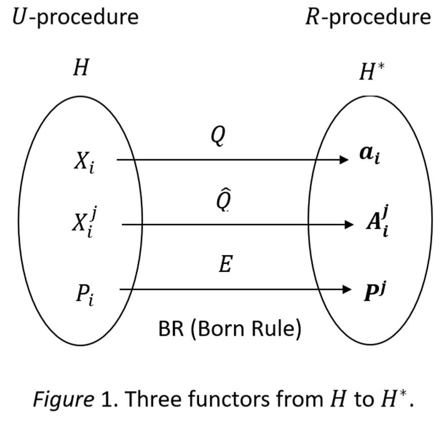
8]. Both 𝐻 and 𝐻∗ can be treated as categories and various operators can be treated as functors between them. In Figure 1, it shows three functors from

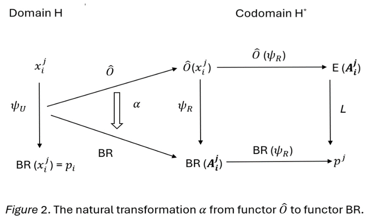
Further, natural transformations exist between these functors. Figure 2 depicts a natural transformation from 𝑄̂ to 𝐵𝑅, where stands for the functor from to the corresponding testing sample , and BR stands for the Born rule, which serves as the bidirectional functor connecting .

The meaning of each symbol in the Figure 2 is defined in
Section 3. The structures of the Figure 2 are explained fully in 6.2.
6.2. Metalogic
It is better to have a holistic picture on the work presented in this paper from metalogical perspectives. To follow the concepts in metalogic, by keeping Gödel’s methods [
6] in mind, we introduce the ideas about metaproperties, namely, consistency and completeness, and prove two theorems accordingly.
Definition 10 (consistency).
Assume the Born probability of an any given testing sample . The U-R model is consistent if the can be inferred from .
Theorem 3. The new U-R model is consistent.
Definition 11 (inverse operators).
For each operator ( introduced earlier, we now introduce its corresponding invers operator respectively: , As usual, for example, .
Definition 12 (completeness).
Assume the Born probability of an any given testing sample . The U-R model is complete if can be inferred from .
Theorem 4. The new U-R model is complete.
Proof.
From Theorems 3 and 4, we can see that the new U-R model for the evolution of the Schrödinger equation is consistent and complete. Thus, we may conclude that the open conjecture of the so-called measurement paradox, i.e., the U-procedure verses the R-procedure, of the quantum mechanics is closed.
7. General discussions
In its very nature, physics is an empirical science. Thus, the measurement problem must be taken seriously. In this paper, we constructed a novel stochastic sampling model, which enabled us to formulate a reasonable solution to the measurement paradox that has long been impeding the development of quantum mechanics. The revised version of Schrödinger equation should have a wide effect on the foundations of quantum theoretic modeling. Below are some further research directions.
First, to make the framework presented here relativistic, such that we may have a new picture of quantum field theory. It is also worth mentioning that sampling is actually a kind of localization.
Second, to extend the stochastic sampling approach to statistical physics, such that we may build a bridge to stochastic thermodynamics [
9].
In addition, the measurement problem is a problem shared by a wide range of scientific fields. To list a few, each of the following domains commonly performs a version of the Yes/No measurement: psychology of reasoning, standard educational test, behavioral science, the Turing test, deep learning and big data models, etc. As John Wheeler once pointed out, quantum theoretic measurements are likely playing the 20-questions game with nature. It is a deep insight. As long as we are concerned with quantum observations and working on empirical issues involving micro-phenomenon, it is necessary to construe this character into our theoretical framework and corresponding models.
Theoretically, this paper contributes two key concepts, both of which generated from the stochastic sampling model: the sample phase and the phase potential. In quantum dynamic analysis of particle physics, we know that there are two kinds of phases, namely, the internal dynamic phase carried by the wavefunction and the external Berry phase for parallel transport. We add a third kind of statistical phase, namely, the sample phase. The potential term in the classical Schrödinger equation captures the difference of space points. In the revised Schrödinger equation, not only does the potential term reflect the difference between the yes-number and the no-number within a sample, but it also provides the information on the difference from one sample to another. We are confident that these new perspectives will have many applications.
Acknowledgments
My special gratitude is to Roger Penrose. It is his insightful thinking and careful analysis on the measurement problem (paradox, in his word) that originally leads to the work presented here. I also thank Hongbin Wang for clarifying some issues in category theory.
References
- R. Penrose (2004), The Road to Reality: A Complete Guide to the Laws of Universe. Random House Inc., New York.
- von Neuman (1955/1983), The Foundations of Quantum Mechanics. Princeton University Press, Princeton, New Jersey.
- J. J. Sakurai (1993), Modern Quantum Mechanics. Addison Wesley Longman, Boston, MA.
- D. H. Griffel (1981/2002), Applied Functional Analysis. Dover Publications, Inc. Mineola, New York.
- P. A. M. Dirac (1930/1958), Principles of Quantum Mechanics. Oxford University Press, Pearson Education, Inc. , New York.
- Y. Yang (2020/2023), Logical foundations of local gauge symmetry and symmetry breaking. arXiv:2004.13582 (math). Journal of Human Cognition, Issue 2, 2023.
- R. P. Feynman, R. B. Leighton, and M. Sands (1989), The Feynman Lectures on Physics. Pearson Education, Addison Wesley, Boston, MA.
- T. Leinster (2014/2017), Basic Category Theory. Cambridge University Press, New York.
- L. Peliti and S. Pigolotti (2021), Stochastic Thermodynamics: An Introduction. Princeton University Press, Princeton, New Jersey.
|
Disclaimer/Publisher’s Note: The statements, opinions and data contained in all publications are solely those of the individual author(s) and contributor(s) and not of MDPI and/or the editor(s). MDPI and/or the editor(s) disclaim responsibility for any injury to people or property resulting from any ideas, methods, instructions or products referred to in the content. |
© 2024 by the authors. Licensee MDPI, Basel, Switzerland. This article is an open access article distributed under the terms and conditions of the Creative Commons Attribution (CC BY) license (http://creativecommons.org/licenses/by/4.0/).


